The higher-order spectrum of simplicial complexes:
 a renormalization group approach

Abstract

Network topology is a flourishing interdisciplinary subject that is relevant for different disciplines including quantum gravity and brain research. The discrete topological objects that are investigated in network topology are simplicial complexes. Simplicial complexes generalize networks by not only taking pairwise interactions into account, but also taking into account many-body interactions between more than two nodes. Higher-order Laplacians are topological operators that describe higher-order diffusion on simplicial complexes and constitute the natural mathematical objects that capture the interplay between network topology and dynamics. We show that higher-order up and down Laplacians can have a finite spectral dimension, characterizing the long time behaviour of the diffusion process on simplicial complexes that depends on their order $m$. We provide a renormalization group theory for the calculation of the higher-order spectral dimension of two deterministic models of simplicial complexes: the Apollonian and the pseudo-fractal simplicial complexes. We show that the RG flow is affected by the fixed point at zero mass, which determines the higher-order spectral dimension $d_{S}$ of the up-Laplacians of order $m$ with $m\geq 0$.

1 Introduction

Simplicial complexes [1, 2, 3, 4, 5, 6] are generalized network structures that capture many-body interactions. They are not just formed by nodes and links like networks but they also include simplices of higher dimensions such as triangles, tetrahedra and so on. Being build by these topological building blocks, simplicial complexes are the ideal discrete structures to investigate emergent geometry [7, 8, 9, 10, 11] and can be described by discrete algebraic and combinatorial topology. Topology is a traditional tool of high-energy physics and quantum gravity and recently it has also become increasingly popular to investigate complex systems[12]. In fact topological methods have been shown to be very powerful to analyse datasets, including brain networks and collaboration networks [13, 14, 2, 15]. Finally there is an increasing interest in revealing the role that the higher-order interactions of simplicial complexes have on their dynamics [16, 17, 19, 20, 21, 22].

The network Laplacian [23, 24, 25, 26] is fundamental to understand the interplay between topology and dynamics and its spectral properties are known to affect diffusion and synchronization on network structures. In particular the spectral dimension [27, 28, 29, 30, 31, 32, 33, 34, 35, 36] characterizes the spectral properties of networks with distinct geometrical features and determines the late time behavior of diffusion and more general dynamical processes on networks [37, 38, 39, 40, 41]. The spectral dimension can also be defined on simplicial complexes [28] by focusing on their skeleton (the network obtained from a simplicial complex by retaining only its nodes and links). Thus, the spectral dimension is also considered a key mathematical object for investigating the effective dimension of a simplicial quantum geometry as felt by diffusion processes. More in general in quantum gravity the spectral dimension is used for probing the geometry of the simplicial spacetimes [42, 43, 44] described by different theoretical approaches including Causal-Dynamical-Triangulations (CDT) [45].

Here we focus on two models of pure $d$-dimensional simplicial complexes called Apollonian simplicial complexes,[46, 47, 48] and pseudo-fractal simplicial complexes [49]. The Apollonian simplicial complexes [46, 47, 48] are deterministic hyperbolic $d$-dimensional manifolds that are obtained by an iterative process, whose limit converges to an infinite hyperbolic lattice. The Apollonian simplicial complex in $d$-dimensions is dominated by the boundary and is closely related to the melonic graphs of tensor networks [50, 51], because melonic graphs can be understood as the merging of two identical Apollonian simplicial complexs upon identification of the all their faces at the boundary. The pseudo-fractal simplicial complexes [49], generalise the Apollonian simplicial complexes to simplicial complexes that are not manifolds. These deterministic simplicial complexes have a skeleton which is non-amenable, i.e. they have an infinite isoperimetric dimension and simultaneously have a very small Cheeger constant [52, 53]. Additionally, they are small world and scale-free.

While the Apollonian and the pseudo-fractal simplicial complexes are generated iteratively by a deterministic algorithm, most of the real networks are the outcome of a stochastic process. In is therefore important to note that the two classes of simplicial complexes considered here constitute the backbone of the more general simplicial complex model called “Network Geometry with Flavor” [8, 9, 11]. This model generates random simplicial complexes whose structure evolves according to a stochastic process, where the set of possible simplices is restricted to be a depending on the model parameters either a subset of the faces of the Apollonian simplicial complex or a subset of the pseudo-fractal simplicial complexes.

Given the fact that Apollonian and pseudo-fractal simplicial complexes are highly geometrical, deterministic and hierarchical, these structures and their generalizations [55, 56] are very suitable for conducting renormalization group (RG) calculations analytically. Examples of dynamical processes already studied with the RG in related simplicial complex models include percolation[57, 58, 59, 60, 61, 62], spin models [63] and Gaussian models [28, 29, 30].

In this paper we investigate the properties of higher-order Laplacians [64, 65, 66, 17, 52, 53] on the considered simplicial complexes. The higher-order Laplacians describe diffusion processes occurring on higher-order simplices [64, 17] and are key mathematical objects to define the higher-order Kuramoto model [18]. Higher order Laplacians are also closely related to approximate Killing vector fields, which are currently being investigated on quantum geometries in CDT [67]. It has been recently shown numerically [17], that the higher-order up-Laplacian and down-Laplacian can display a finite spectral dimension. Here we use renormalization group (RG) theory [28, 29, 30] to analytically calculate the spectral dimension of higher-order up-Laplacians of Apollonian and pseudo-fractal simplicial complexes. We find that each simplicial complex belonging to the considered class of models, is characterized by a set of analytically predicted spectral dimensions. Each spectral dimension corresponds to the spectrum of a higher-order up-Laplacian of different order $m$. The values of the predicted spectral dimensions are compared to direct numerical results for $d=3$ and $d=4$ simplicial complexes.

The paper is structured as follows: in Sec. II we introduce simplicial complexes and their higher-order Laplacians, in Sec.III we present the hyperbolic and non-amenable simplicial complex models considered in this work; in Sec. III we give the necessary background for deriving the higher-order spectrum of the Apollonian and pseudo-fractal simplicial complexes using the RG approach; In Sec. IV and in Sec. V we derive the RG equations and the RG flow for the Apollonian simplicial complexes; In Sec. VI and Sec. VII we derive the RG equations and the RG flow for the pseudo-fractal simplicial complexes. In Sec. VIII we summarize the main analytical results and we will compare with numerical results on all the considered simplicial complex models. Finally, in Sec. IX we will provide the conclusions.

2 Simplicial complexes and higher-order Laplacians

2.1 Simplicial complexes

A $m$-dimensional simplex $r$ (also indicated as $m$-simplex) includes $m+1$ nodes and it can be indicated as

$$r=[v_{0},v_{1},\ldots,v_{m}].$$ (1)

Therefore, a $0$-simplex is a node, a $1$-simplex is a link, a $2$-simplex a triangle, a $3$-simplex a tetrahedron and so on. A $m^{\prime}$-dimensional face $q$ of a $m$-dimensional simplicial complex $r$ is a $m^{\prime}<m$ simplex formed by a subset of $m^{\prime}+1$ nodes belonging to the simplex $r$.

In topology, simplices also have an orientation. Two $m$-simplices differing only by the order in which their nodes are listed are therefore related by

$$[v_{0},v_{1},\ldots,v_{m}]=(-1)^{\sigma(\pi)}[v_{\pi(0)},v_{\pi(1)},\ldots,v_{\pi(m})],$$ (2)

where $\sigma(\pi)$ indicates the parity of the permutation $\pi$ of the $m+1$ indices of the nodes.

A simplicial complex is formed by a set of simplices with the property that the simplicial complex is closed under inclusion of the faces of any of its simplices.

A $d$-dimensional simplicial complex is a simplicial complex for which the maximum dimension of its simplices is $d$. Here we are exclusively interested in pure $d$-dimensional simplicial complexes, which are formed by a set of $d$-dimensional simplices and all their faces. The skeleton of a simplicial complex is the network formed by the set of all the nodes and links of the simplicial complex. Given a $d$-dimensional simplex, we indicate the number of its $m$-simplices with $N^{[m]}$ with $0\leq m\leq d$.

2.2 Boundary map and incidence matrices

Given a simplicial complex, a $m$-chain consists of the elements of a free abelian group $\mathcal{C}_{m}$ with basis formed by the set of all $m$-simplices of the simplicial complex. Therefore every element $a\in\mathcal{C}_{m}$ can be uniquely expressed as a linear combination of basis elements with coefficients given $c_{r}\in\mathbb{Z}_{2}$, i.e.

$$a=\sum_{r\in{Q}^{[m]}}c_{r}\left[v_{0}^{(r)},v_{1}^{(r)},\ldots,v_{m}^{(r)}\right]$$ (3)

where $c_{r}\in\{1,-1\}$. Here ${Q}^{[m]}$ indicates the set of all $m$-simplices of the simplicial complex and each $m$-simplex $r\in{Q}^{[m]}$ of the simplicial complex is indicated by $r=[v_{0}^{(r)},v_{1}^{(r)},\ldots,v_{m}^{(r)}]$.

The boundary map $\partial_{m}$ is a linear operator $\partial_{m}:\mathcal{C}_{m}\to\mathcal{C}_{m-1}$ whose action is determined by the action on each $m$-simplex of the simplicial complex. In particular the boundary map $\partial_{m}$ applied to the $m$ simplex $r=[v_{0},v_{1},\ldots,v_{m}]$ gives

$$\partial_{m}[v_{0},v_{1}\ldots,v_{m}]=\sum_{j=0}^{m}(-1)^{j}[v_{0},v_{1},\ldots,v_{j-1},v_{j+1},\ldots,v_{m}].$$ (4)

In words, the boundary map applied to a $m$-simplex gives a linear combinations of its $(m-1)$-dimensional faces.

We say that two $m$-faces $r$ and $q$ of a simplicial complex are upper adjacent if there is a $(m+1)$-simplex $\tau$ of which both $r$ and $q$ are faces. The $m$-faces $r$ and $q$ are upper adjacent with similar orientation if the simplicial complex contains a $(m+1)$-dimensional simplex $\tau$ such that

$$\langle{r,\partial_{m+1}\tau}\rangle=\langle{q,\partial_{m+1}\tau}\rangle,$$ (5)

where $\langle a,b\rangle$ indicates the inner product on $\mathcal{C}_{m}$. Conversely, they are upper adjacent with opposite orientation if the simplicial complex contains a $(m+1)$-dimensional simplex $\tau$ such that

$$\langle{r,\partial_{m+1}\tau}\rangle=-\langle{q,\partial_{m+1}\tau}\rangle.$$ (6)

From the definition of the boundary map $\partial_{m}$ given by Eq. (4), it follows immediately that for every $m$-dimensional simplex $r$

$$\partial_{m-1}\partial_{m}r=0,$$ (7)

which is an important topological property that can be expressed in words with the sentence “the boundary of a boundary is null”.

Given a simplicial complex with $N^{[m]}$ $m$-dimensional simplices we can choose a base for ${\mathcal{C}}_{m}$ by taking an ordered list of its $m$ simplices. If we fix both the base of ${\mathcal{C}}_{m}$ and ${\mathcal{C}}_{m-1}$ we can represent the boundary operator $\partial_{m}$ by a $N^{[m-1]}\times N^{[m]}$ incidence matrix ${\bf B}_{[m]}$. In Figure 1 we show an example of a simplicial complex. We choose as bases for ${\mathcal{C}}_{0},{\mathcal{C}}_{1}$ and ${\mathcal{C}}_{2}$ the ordered list of nodes $\{[1],[2],[3],[4]\}$, links $\{[1,2],[1,3],[2,3],[3,4],[2,4]\}$ and triangles $\{[123],[234]\}$. With this choice of bases, the boundary maps $\partial_{1}$ and $\partial_{2}$ can be represented by the incidence matrices ${\bf B}_{[1]}$ and ${\bf B}_{[2]}$ with,

$${\bf B}_{[1]}=\left(\begin{array}[]{ccccc}-1&-1&0&0&0\\ 1&0&-1&0&-1\\ 0&1&1&-1&0\\ 0&0&0&1&1\\ \end{array}\right),\ {\bf B}_{[2]}=\left(\begin{array}[]{cc}1&0\\ -1&{0}\\ 1&{1}\\ 0&1\\ {0}&{-1\par}\end{array}\right).$$ (17)

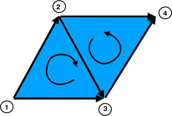
Figure 1: An example of a small simplicial complex with the orientation of the simplices induced by the labelling of the nodes.

2.3 Higher order Laplacian matrices of simplicial complexes

The graph Laplacian or $0$-Laplacian describes the diffusion process over a network and it is an extensively studied topological operator in graph theory [23]. The $0$-Laplacian can be also defined for a simplicial complex and describes the diffusion process that goes from a node to another node across shared links. In fact the $0$-Laplacian is a $N^{[0]}\times N^{[0]}$ matrix and can be expressed in terms of the incidence matrix ${\bf B}_{[1]}$,

$${\bf L}_{[0]}={\bf B}_{[1]}{\bf B}^{\top}_{[1]}.$$ (18)

While on networks only the graph Laplacian and its normalized versions can be defined, in simplicial complexes it is possible to define higher-order Laplacians describing diffusion taking place between higher-order simplices. The higher-order Laplacian ${\bf L}_{[m]}$ with $m>0$ (also called combinatorial Laplacians) can be represented as a $N^{[m]}\times N^{[m]}$ matrix given by

$${\bf L}_{[m]}={\bf L}_{[m]}^{down}+{\bf L}_{[m]}^{up},$$ (19)

where ${\bf L}_{[m]}^{down}$ and ${\bf L}_{[m]}^{up}$ are the down-Laplacian and the up-Laplacian of order $m$ and are defined as

$${\bf L}_{[m]}^{down} = {\bf B}^{\top}_{[m]}{\bf B}_{[m]},$$

$${\bf L}_{[m]}^{up} = {\bf B}_{[m+1]}{\bf B}^{\top}_{[m+1]}.$$ (21)

The down-Laplacian ${\bf L}_{[m]}^{down}$ of order $m$, describes diffusion process taking place among $m$ simplices across $(m-1)$ shared simplices. For instance, the down-Laplacian of order $1$ describe diffusion from link to link across shared nodes. The up-Laplacian ${\bf L}_{[m]}^{up}$ of order $m$ describes diffusion processes taking place among $m$ simplices across shared $(m+1)$ simplices. The up-Laplacian of order $1$ for example, describes the diffusion from link to link across shared triangles.

Interestingly the spectral properties of the higher-order Laplacians can be proven to be independent on the orientation of the simplices as long as the orientation is induced by a labelling of the nodes.

One of the main results of Hodge theory [65, 16, 17] is that the degeneracy of the zero eigenvalues of the $m$- Laplacian ${\bf L}_{[m]}$ is equal to the Betti number $\beta_{m}$. The corresponding eigenvectors localize around the corresponding $m$-dimensional cavity of the simplicial complex. It follows that if the simplicial complex has trivial topology, i.e. it is formed by a single connected component, $\beta_{0}=1$ and the simplicial complex has no higher-order cavities, (i.e. $\beta_{m}=0$ for all $m>0$) then the $0$-Laplacian ${\bf L}_{[0]}$ has a zero eigenvalue that is not degenerate while all the higher-order Laplacians ${\bf L}_{[m]}$ with $m>0$ do not admit any zero eigenvalue.

Let us observe here that Eq. (7) can be expressed in terms of the incidence matrices as

$${\bf B}_{[m-1]}{\bf B}_{[m]} = {\bf 0},$$

$${\bf B}^{\top}_{[m]}{\bf B}^{\top}_{[m-1]} = {\bf 0}.$$ (22)

From these relations it can be easily shown that the eigenvectors associated to the non-null eigenvalues of ${\bf L}^{up}_{[m]}={\bf B}_{[m+1]}{\bf B}^{\top}_{[m+1]}$ are orthogonal to the eigenvectors associated with the non-null eigenvalues of ${\bf L}^{down}_{[m]}={\bf B}^{\top}_{[m]}{\bf B}_{[m]}$. Hodge theory therefore demonstrates (see for instance [16] for a gentle introduction) that the spectrum of the $m$-Laplacian includes all the non-null eigenvalues of the $m$-up-Laplacian and all the non-null eigenvalues of the $m$-down Laplacian. The other eigenvalues of the $m$-Laplacian can only be zero and their degeneracy is given by the Betti number $\beta_{m}$. Therefore the spectrum of the $m$-Laplacian is completely determined once the spectra of both the $m$-up-Laplacian and the $m$-down-Laplacian are known.

Finally we observe that the up-Laplacians and the down-Laplacians are related by transposition

$${\bf L}_{[m]}^{up}=[{\bf L}_{[m+1]}^{down}]^{\top}.$$ (23)

Therefore the spectrum of the $m$-up Laplacian is equal to the spectrum of the $(m+1)$-down Laplacian.

Taking all these consideration together it follows that in order to know the spectrum of all higher-order Laplacians of a simplicial complex it is sufficient to know the spectrum of all its higher-order up-Laplacians.

Therefore in this work, without loss of generality we will focus on the spectral properties of $m$-up-Laplacians of pure $d$-dimensional simplicial complexes with order $0\leq m<d-1$.

2.4 Up-Laplacians and their spectral dimension

For a simplicial complex of dimension $d>m$ it is possible to define both a normalized and an un-normalized higher-order up $m$-Laplacian. The un-normalized higher order up-Laplacian ${\bf{L}}^{up}_{[m]}={\bf B}_{[m+1]}{\bf B}^{\top}_{[m+1]}$ has elements

$$[{L_{[m]}^{up}}]_{rq}=k_{r}^{[m]}\delta_{r,q}-\left(a^{[m]}_{\mathbin{\uparrow}\downarrow}\right)_{rq}+\left(a_{\upuparrows}^{[m]}\right)_{rq},$$ (24)

where ${\delta}_{x,y}$ indicates the Kronecker delta. In Eq. (24) we have used the oriented upper incidence matrices ${\bf a}^{[m]}_{\mathbin{\uparrow}\downarrow}$ and ${\bf a}^{[m]}_{\upuparrows}$ defined as follows: $(a_{\upuparrows}^{[m]})_{rq}=1$ if the two $m$-dimensional faces $r$ and $q$ are upper adjacent (they are both incident to a $(m+1)$-dimensional simplex) and have similar orientation, otherwise $(a_{\upuparrows}^{[m]})_{rq}=0$; similarly $(a_{\mathbin{\uparrow}\downarrow}^{[m]})_{rq}=1$, if the two $m$-dimensional faces $r$ and $q$ are upper adjacent (they are both incident to a $(m+1)$-dimensional simplex) and have dissimilar orientation, otherwise $(a_{\mathbin{\uparrow}\downarrow}^{[m]})_{rq}=0$. Finally $k_{r}$ indicates the number of $(m+1)$-dimensional simplices incident to the $m$-dimensional simplex $r$.

The up-Laplacian can be used to characterize diffusion occurring among higher-order simplicies. In particular the spectral properties of up-Laplacians can affect the relaxation time of the diffusion process as discussed in Ref. [17] for the simplicial complex model called “Network Geometry with Flavor”.

Let us define the $N^{[m]}\times N^{[m]}$ matrix ${\bf K}_{[m]}$ as the diagonal matrix with diagonal elements $[{\bf K}_{[m]}]_{rr}=[L^{up}_{[m]}]_{rr}$. The normalized $m$-up-Laplacian $\hat{\bf L}_{[m]}^{up}$ can be defined as

$$\hat{\bf L}_{[m]}^{up}={\bf K}_{[m]}^{-1/2}{\bf L}^{up}_{[m]}{\bf K}_{[m]}^{-1/2},$$ (25)

where we note that in this expression we use the convention $0/0=0$. The normalized $m$-up-Laplacian ${\hat{\bf L}}_{[m]}^{up}$ has elements

$$[{\hat{L}_{[m]}}^{up}]_{rq}=\delta_{r,q}-\frac{1}{\sqrt{k_{r}^{[m]}k_{q}^{[m]}}}\left(a^{[m]}_{\mathbin{\uparrow}\downarrow}\right)_{rq}+\frac{1}{\sqrt{k_{r}^{[m]}k_{q}^{[m]}}}\left(a_{\upuparrows}^{[m]}\right)_{rq}.$$ (26)

In this work we will focus on the spectral properties of the normalized up-Laplacians. The spectrum of the normalized and un-normalized $m$-up-Laplacians is in general distinct for simplicial complexes in which $k_{r}$ is dependent on $r$. However, we anticipate that when they both display a spectral dimension, their spectral dimension is the same [31].

The density of eigenvalues $\bar{\rho}(\mu)$ of the normalized $m$-up-Laplacian has a density of eigenvalues that includes a singular part formed by a delta function at $\mu=0$ and a regular part ${\rho}(\mu)$, i.e.

$$\bar{\rho}(\mu)=\bar{\rho}(0)\hat{\delta}(\mu)+{\rho}(\mu),$$ (27)

where we use $\hat{\delta}(x)$ to denote the delta function. The emergence of the delta peak at $\mu=0$ can be easily explained. First let us observe that Eq. (25) implies that the number of zero eigenvalues of the normalized and un-normalized $m$-up-Laplacians is the same. Secondly let us note that the spectrum of the $m$-up-Laplacian ${\bf L}^{up}_{[m]}$ can contain a highly degenerate zero eigenvalue. In fact, given the definition of the $m$-up-Laplacian ${\bf L}^{up}_{[m]}={\bf B}_{[m+1]}{\bf B}^{\top}_{[m+1]}$ it follows that the eigenvalues of the $m$-up-Laplacian are the square of the singular values of the incidence matrix ${\bf B}_{[m+1]}$. Since the incidence matrix ${\bf B}_{[m+1]}$ is a rectangular $N^{[m]}\times N^{[m+1]}$ matrix, the non-zero singular values cannot be more than $\min(N^{[m]},N^{[m+1]})$. In particular for simplicial complexes with trivial topology, the Hodge decomposition [16] implies that the number of non-zero eigenvalues of the $m$-up-Laplacian with $m>0$ are given by $\hat{N}^{[m]}=\min(N^{[m]},N^{[m+1]})$. It follows that all the other eigenvalues are zero. Therefore for $m>0$ the degeneracy of the zero eigenvalue can be extensive, while for $m=0$ the degeneracy of the zero eigenvalue is given by the Betti number $\beta_{0}$, where $\beta_{0}=1$ for a trivial topology. For a trivial topology the density of eigenvalues at $\mu=0$ of the graph Laplacian ($m$-up-Laplacian with $m=0$) is zero in the large network limit, while it can be greater than zero for $m>0$.

The normalized $m$-up Laplacian displays a finite spectral dimension $d_{S}$ when the regular part of its density of eigenvalues $\bar{\rho}(\mu)$ obeys the asymptotic behaviour

$$\rho(\mu)\cong C\mu^{d_{S}/2-1},$$ (28)

where $\mu\ll 1$ and $C$ is independent of $\mu$.

From this scaling it directly follows that the cumulative distribution ${\rho}_{c}(\mu)$ of the regular part of the density of eigenvalues ${\rho}(\mu)$, which is the integral of the density of eigenvalues $0<\mu^{\prime}\leq\mu$, follows the scaling

$${\rho}_{c}(\mu)\cong\tilde{C}\mu^{d_{S}/2},$$ (29)

for $\mu\ll 1$. This relation will prove useful in the following, when we will numerically compare the predicted spectral dimension with the numerical results.

3 Simplicial complexes under consideration

3.1 Apollonian simplicial complexes of any dimension

A $d$-dimensional Apollonian simplicial complex [46, 47] (with $d\geq 2$) is generated iteratively by starting from a single $d$-simplex at generation $n=0$ and adding a $d$-simplex at each generation $n>0$ to every $(d-1)$-dimensional face introduced at the previous generation. In Figure 2a we show a $d=2$ dimensional Apollonian simplicial complex at iteration $n=2$.

Figure 2: The $d=2$ dimensional Apollonian (panel (a)) and pseudo-fractal (panel (b)) simplicial complexes are shown at iteration $n=2$. The triangles added at iteration $n=0,1,2$ are shown in color blue, red and cyan respectively.

3.2 Higher order Laplacian matrices of simplicial complexes

At generation $n=0$ there are $N_{0}^{[m]}$ $m$-dimensional simplices in the simplicial complex with

$$N_{0}^{[m]}={{d+1}\choose{m+1}}.$$ (30)

The number ${\mathcal{N}}_{n}^{[m]}$ of $m$-dimensional faces at generation $n$ is given by

$${\mathcal{N}}_{n}^{[m]}=(d+1)d^{n-1}{d\choose m}$$ (31)

In these Apollonian simplicial complexes, there are $N_{n}^{[m]}$ $m$-dimensional simplicial complexes at generation $n$ with

$$N_{n}^{[m]} = N_{0}^{[m]}+\sum_{n^{\prime}=1}^{n}{\mathcal{N}}_{n^{\prime}}^{[m]}=(d+1)\left[\frac{d^{n}-1}{d-1}+\frac{1}{m-1}\right]{{d}\choose m},$$ (32)

Finally we note here that in the following we will used the notation $Q^{[m]}$ to indicate the set of $m$-simplices of the Apollonian simplicial complex.

The Apollonian simplicial complex are small-world, i.e. their skeleton has an infinite Hausdorff dimension,

$$d_{H}=\infty,$$ (33)

therefore at each generation their diameter grows logarithmically with the total number of nodes of the network. Moreover, the Apollonian simplicial complex of dimension $d$ are manifolds that define discrete hyperbolic lattices including for $d=2$ the Farey graph.

Let us add here a pair of additional combinatorial properties of Apollonian simplicial complex that will be useful later. At each generation $n$ we call simplices of type $\ell$ the simplices added at generation $n^{\prime}=n-\ell$. At generation $n$, the number of $d$-simplices of generation $n$ attached to simplices of dimension $m$ (with $m<d$) of type $\ell>0$ is given by

$$w_{\ell}^{[m]}=(d-m)(d-m-1)^{\ell-1}.$$ (34)

Moreover, we observe that the number of $(m+1)$-dimensional simplices of generation $n$ incident to $m$-simplices added at generation $n^{\prime}=n-\ell$ is given by $w_{\ell}^{[m]}$ for $\ell>0$ and $w_{\ell}^{[m]}=d-m$ for $\ell=0$.

3.3 Pseudo-fractal simplicial complexes of any dimension

A pseudo-fractal simplicial complex [49] of dimension $d$ with $d\geq 2$ is constructed iteratively. At generation $n=0$ the simplicial complex is formed by a single $d$-simplex (with $d\geq 2$). At each generation $n>0$ we glue a $d$-simplex to every $(d-1)$-dimensional face introduced at generation $n\geq 0$. In Figure 2b we show a of $d=2$ dimensional pseudo-fractal simplicial complex at iteration $n=2$. At generation $n=0$ the number of $m$-dimensional simplices ${N}_{0}^{[m]}$ is given by

$$N_{0}^{[m]}={{d+1}\choose{m+1}}.$$ (35)

The number ${\mathcal{N}}_{n}^{[m]}$ of $m$-dimensional faces added at generation $n>0$ is given by

$${\mathcal{N}}_{n}^{[m]}=(d+1)^{n}{d\choose{m}}.$$ (36)

The number $m$-dimensional faces $N_{n}^{[m]}$ at generation $n$ is

$$N^{[m]}_{n} = N_{0}^{[m]}+\sum_{n^{\prime}=1}^{n}{\mathcal{N}}_{n^{\prime}}^{[m]}$$ (37)

$$= (d+1)\left[\frac{(d+1)^{n}-1}{d}+\frac{1}{m+1}\right]{d\choose{m}}.$$

The pseudo-fractal simplicial complexes differs from Apollonian simplicial complexes significantly as they are not discrete manifolds. However both simplicial complexes have an underlying non-amenable network structure and are characterized by having a small Cheeger constant.

Moreover the pseudo-fractal simplicial complexes, as the Apollonian simplicial complexes, have a small-world skeleton, i.e. their underlying networks have an infinite Hausdorff dimension

$$d_{H}=\infty.$$ (38)

For pseudo-fractal simplicial complexes we use the same notation as for Apollonian simplicial complex and we indicate $Q^{[m]}$ the set of $m$-simplices of the pseudo-fractal simplicial complex. Additionally we indicate as simplices of type $\ell$ the simplices added at generation $n^{\prime}=n-\ell$, in the pseudo-fractal simplicial complex evolved up to generation $n$. We make the following useful remark: at generation $n$ the number of $d$-simplices of generation $n$ attached to $m$-simplices (with $m<d$) of type $\ell>0$ is given by

$$\hat{w}_{\ell}^{[m]}=(d-m)\sum_{\ell^{\prime}=0}^{\ell}(d-m-1)^{\ell^{\prime}-1}.$$ (39)

Finally the number of $(m+1)$-simplices of generation $n$ added to $m$-simplices of generation $n^{\prime}=n-\ell$ is given by $\hat{w}_{\ell}^{[m]}$ for $\ell>0$ and $\hat{w}_{0}^{[m]}=(d-m)$ for $\ell=0$.

4 Gaussian model and the RG approach

4.1 The ensemble of weighted normalized Laplacians

In this section our goal is to define the theoretical framework of a real space RG approach to calculate the spectrum of the normalized $m$-dimensional up-Laplacian of the Apollonian and the pseudo-fractal simplicial complexes. The renormalization group acts on a weighted simplicial complex in which we attribute a weight $p_{\tau}$ to each $(m+1)$-dimensional simplex $\tau$ while the topology of the simplicial complex remains fixed. Therefore in the RG approach we investigate the RG flow defined over the ensemble of weighted normalized up-Laplacian matrices ${\bf\hat{L}}_{[m]}^{up}$ of elements

$$[\hat{L}_{[m]}^{up}]_{rq}=\delta_{r,q}-\frac{1}{\sqrt{s_{r}^{[m]}s_{q}^{[m]}}}p_{\tau(r,q)}\left(a^{[m]}_{\mathbin{\uparrow}\downarrow}\right)_{rq}+\frac{1}{\sqrt{s_{r}^{[m]}s_{q}^{[m]}}}p_{\tau(r,q)}\left(a_{\upuparrows}^{[m]}\right)_{rq},$$ (40)

where $p_{\tau(qr)}$ indicates the weight of the $(m+1)$-dimensional simplex $\tau$ incident to both $r$ and $q$ and $s_{r}$ indicates the strength of the simplex $r$, i.e. $s_{r}=\sum_{\tau\supset r}^{N_{n}^{[m+1]}}p_{\tau}$. From here on, we will focus on finding the density of eigenvalues of the up-Laplacian of order $m$. In the following sections we will therefore adopt a simplified notation, dropping the indication ”up” and the index $[m]$ in most of the relevant mathematical quantities. We will therefore indicate ${\bf\hat{L}}_{[m]}^{up}$ simply as ${\bf\hat{L}}$, $N_{n}^{[m]}$ as $N_{n}$, $a^{[m]}_{\mathbin{\uparrow}\downarrow}$ as $a_{\mathbin{\uparrow}\downarrow}$, $a_{\upuparrows}^{[m]}$ as $a_{\upuparrows}$ and so on.

4.2 Gaussian models and Laplacian spectrum

The density of eigenvalues of a symmetric matrix can be derived analytically using the properties of the Gaussian model following a standard procedure of statistical mechanics [29] quite common in Random Matrix Theory [69, 68]. Therefore if we want to derive the density of eigenvalues of the $m$-dimensional up-Laplacian $\hat{{\bf L}}$ which for generation $n$ will be a $N_{n}\times N_{n}$ symmetric matrix we should consider the Gaussian model whose partition function reads

$$Z(\mu)=\int{\mathcal{D}}\psi\exp\left[i\mu\sum_{r}\psi_{r}^{2}-i\sum_{rq}\hat{L}_{rq}\psi_{r}\psi_{q}\right]=\frac{(i\pi)^{N_{n}/2}}{\sqrt{\prod_{r}(\mu-\mu_{r})}},$$ (41)

where $\mu_{r}$ are the eigenvalues of the normalized up-Laplacian matrix $\hat{\bf L}$ and the differential ${\mathcal{D}}\psi$ stands for

$${\mathcal{D}}\psi=\prod_{r=1}^{N_{n}}\left(\frac{d\psi_{r}}{\sqrt{2\pi}}\right).$$ (42)

By changing variables and putting $\phi=\psi/\sqrt{s_{r}}$ the partition function can be rewritten as

$$Z(\mu)=\prod_{r=1}^{N_{n}}\sqrt{s_{r}}\int{\mathcal{D}}\phi e^{iH(\{\phi\})},$$ (43)

with

$$H(\{\phi\})=\sum_{\tau\in Q^{[m+1]}}p_{\tau}\left[-(1-\mu)\sum_{r\subset\tau}\phi_{r}^{2}+2\sum_{r<q|r,q\subset t}(a^{\mathbin{\uparrow}\downarrow}_{rq}-a^{\upuparrows}_{rq})\phi_{r}\phi_{q}\right],$$ (44)

where $r,q$ are both $m$-simplices, i.e. $r,q\in Q^{[m]}$. The spectral density $\bar{\rho}(\mu)$ of the normalized Laplacian matrix can be found using the relation

$$\bar{\rho}(\mu)=-\frac{2}{\pi}\mbox{Im}\frac{\partial f}{\partial\mu},$$ (45)

where $f$ is the free-energy density defined as

$$f=-\lim_{n\to\infty}\frac{1}{N_{n}}\ln Z(\mu).$$ (46)

In fact, inserting Eq. (41) in the Eq. (46) we obtain

$$f=-\lim_{n\to\infty}\left[\frac{1}{N_{n}}\sum_{r=1}^{N}\frac{1}{2}\ln(\mu-\mu_{r})\right]-\frac{1}{2}\ln(i\pi).$$ (47)

Therefore we can show that Eq. (45) is correct by plugging the final expression for $f$ in Eq.(45),

$$\bar{\rho}(\mu)=-\frac{2}{\pi}\mbox{Im}\frac{\partial f}{\partial\mu}=\frac{1}{\pi}\lim_{n\to\infty}\frac{1}{N_{n}}\mbox{Im}\sum_{r=1}^{N_{n}}\frac{1}{\mu-\mu_{r}}=\lim_{n\to\infty}\frac{1}{N_{n}}\sum_{r=1}^{N_{n}}\hat{\delta}({\mu-\mu_{r}}).$$ (48)

4.3 The general RG approach

As was the case in Ref.[28], where the spectrum of the $0$-Laplacian was derived using the RG flow, the parameters $p$ and $\mu$ are renormalized differently for faces of different type $\ell$ when we study the spectrum of the $m$-dimensional up-Laplacian. The partition function $Z_{n}(\bm{\omega})$ corresponding to the Gaussian model of the simplicial complex evolved up to generation $n$ is a function of the parameters $\bm{\omega}=(\{\mu_{\ell}\},\{p_{\ell}\})$, and can be expressed as

$$Z_{n}(\bm{\omega})=\int\mathcal{D}\phi e^{iH(\{\phi\})},$$ (49)

where

$$H(\{\phi\}) = \sum_{\ell=0}^{n}\sum_{\tau\in Q_{n}^{[m+1]}(\ell)}\left[-i(1-\mu_{\ell})p_{\ell}\sum_{r\subset\tau}\phi_{r}^{2}+2ip_{\ell}\sum_{r<q|r\subset\tau,q\subset\tau}(a_{rq}^{\mathbin{\uparrow}\downarrow}-a_{rq}^{\upuparrows})\phi_{r}\phi_{q}\right],$$ (50)

with $Q_{n}^{[m+1]}{(\ell)}$ indicating the set of $(m+1)$-dimensional simplices of type $\ell$ in a simplicial complex evolved up to generation $n$ and with $r,q\in Q^{[m]}$. The Gibbs measure of this Gaussian model is given in terms of the Hamiltonian $H(\{\phi\})$ defined in Eq. (50) as

$$P_{n}(\{\bm{\phi}\})=\frac{1}{Z(\bm{\omega})}e^{iH(\{\phi\})}.$$ (51)

In order to calculate the partition function $Z_{n}(\bm{\omega})$ we adopt a real space renormalization group approach. We will first integrate the Gaussian fields corresponding to the ${\mathcal{N}_{n}}$ $m$-dimensional simplices added to the simplicial complex at generation $n$ and then iteratively integrate over the simplices added at generation $n-1$ and so forth, until all the integrals in the definition of the partition function $Z_{n}(\bm{\omega})$ are performed. More specifically we consider the following real space renormalization group procedure. We start with initial conditions $\mu_{\ell}=\mu$ and $p_{\ell}=1$ for all values of $\ell>0$. At each RG iteration, we integrate over the Gaussian variables $\phi_{\bar{r}}$ associated to simplices $\bar{r}\in{\mathcal{N}_{n}}$ and we rescale the remaining Gaussian variables in order to obtain the renormalized Gibbs measure $P(\{\bm{\phi^{\prime}}\})$ of the same type as Eq. (51) but with rescaled parameters $(\{\mu_{\ell}^{\prime}\},\{p_{\ell}^{\prime}\})$, i.e.

$$P_{n-1}(\{\bm{\phi^{\prime}}\})=\left.\int{\mathcal{D}}\phi^{(n)}P_{n}(\{\bm{\phi}\})\right|_{\bm{\phi^{\prime}}={\bf F}(\{\bm{\phi}\})},$$ (52)

where

$${\mathcal{D}}\phi^{(n)}=\prod_{r\in{\mathcal{N}_{n}}}\left(\frac{d\phi_{r}}{\sqrt{2\pi}}\right).$$ (53)

The fields are rescaled in a way that keeps $p_{1}=1$ at each iteration of the RG flow, i.e. the weight of the $(m+1)$-dimensional faces of type $\ell=1$ is always fixed to one. It follows that at each step of the RG transformation we have

$$H(\{\phi\})\to H^{\prime}(\{\phi^{\prime}\}),$$ (54)

where,

$$H^{\prime}(\{\phi\})=\sum_{\ell=1}^{n-1}\sum_{\tau\in Q_{n-1}^{[m+1]}{(\ell)}}\left\{-(1-\mu_{\ell}^{\prime})p_{\ell}^{\prime}\sum_{r\subset\tau}(\phi_{r}^{\prime})^{2}+2p_{\ell}^{\prime}\sum_{r<q|r,q\subset\tau}[a_{rq}^{\mathbin{\uparrow}\downarrow}-a_{rq}^{\upuparrows}]\phi_{r}^{\prime}\phi_{q}\right\}.$$ (55)

This procedure allows us to determine the renormalization group transformation $R$ acting on the model parameters ${\bm{\omega}}=(\{\mu_{\ell}\},\{p_{\ell}\})$,

$$\bm{\omega}^{\prime}=R\bm{\omega}.$$ (56)

Under the renormalization group flow, the partition function transforms according to

$$Z_{n}(\bm{\omega})=e^{-{N}_{n}g(\bm{\omega})}Z_{n-1}(\bm{\omega}^{\prime}).$$ (57)

By using Eq. (31) and Eq. (36), the free energy density at generation $n$

$$f = -\lim_{n\to\infty}\frac{1}{N_{n}}\ln Z_{n}(\bm{\omega})$$ (58)

can be approximated as

$$f \simeq \sum_{\tau=0}^{\infty}\frac{g(R^{(\tau)}\bm{\omega})}{d^{\tau}},$$ (59)

for the Apollonian simplicial complexes, and as

$$f \simeq \sum_{\tau=0}^{\infty}\frac{g(R^{(\tau)}\bm{\omega})}{(d+1)^{\tau}},$$ (60)

for the pseudo-fractal simplicial complexes.

We will show in the next section that the RG flow for this Gaussian model is determined by the fixed point at $\mu^{\star}=0$. This implies that the spectral dimension of higher-order up-Laplacians is universal [31], i.e. it is the same for normalized and un-normalized up-Laplacians.

5 General RG equations for the Apollonian simplicial complex

5.1 The integral

To derive the renormalization group equations for the Apollonian simplicial complex we need to perform the integration over the Gaussian fields associated to the $m$-simplices added at generation $n$. In the Apollonian simplicial complex, any $d$-simplex of generation $n$ is only incident to $d$-simplices added at previous generations. Specifically, every new $d$-simplex contains a single new node and shares exactly one of its $(d-1)$-faces with the Apollonian simplicial complex at the previous iteration. Therefore the integrations over all $m$-simplices added at iteration $n$ can be performed independently by separately considering the Gaussian fields corresponding to $m$-simplices belonging to different $d$-simplices added at iteration $n$. Consequently in this paragraph we only focus on the integration over the Gaussian fields associated to $m$-simplices belonging to a single $d$-simplex of generation $n$.

In order to perform this integral let us define some notation. Given the generic $d$-simplex $\bar{r}$ added at iteration $n$, i.e. $\bar{r}\in{\mathcal{N}}_{n}$, we indicate with $j$ its most recent node, i.e the single node $j\subset\bar{r}$ of type $\ell=0$. Each $d$-simplex $\bar{r}$ added at generation $n$ contains ${{d}\choose{m}}$ new $m$-simplices added at generation $n$. All these simplices include the node $j$ and $m$ other nodes out of the $d$ nodes of type $\ell>0$ belonging to $\bar{r}$. We will denote the set of these $m$-simplices by ${\mathcal{M}}_{n}$ and the Gaussian fields associated to the $m$-simplices $q\in{\mathcal{M}}_{n}$ by $\bar{\psi}_{q}$. Additionally, the simplex $\bar{r}$ contains ${d}\choose{m+1}$ $m$-faces formed exclusively by nodes of type $\ell>0$. We will denote the set of these simplices by ${\mathcal{R}}_{n}$ and the Gaussian fields associated to the $m$-simplices $q\in{\mathcal{R}}_{n}$ by ${\phi}_{q}$. Finally, let us define ${\mathcal{Q}}^{[m+1]}$ to be the set of all $(m+1)$-dimensional faces of the simplex $\bar{r}$ added at iteration $n$. With this notation, the integral over the fields $\{\bar{\psi}_{\bar{r}}\}$ reads,

$$I_{m}=\int\mathcal{D}\bar{\psi}\ \exp\left\{i\left[H_{0}(\{\bar{\psi}\},\{\phi\})+H_{1}(\{\bar{\psi}\},\{\phi\})\right]\right\},$$ (61)

where $H_{0}(\{\bar{\psi}\},\{\phi\})$ is given by

$$H_{0}(\{\bar{\psi}\},\{\phi\}) = -(1-\mu_{1})\left[(d-m)\sum_{q\in{\mathcal{M}}_{n}}\bar{\psi}_{q}^{2}+\sum_{q\in{\mathcal{R}}_{n}}\phi_{q}^{2}\right],$$ (62)

and $H_{1}(\{\bar{\psi}\},\{\phi\})$ is given by

$$H_{1}(\{\bar{\psi}\},(\{\phi\})=2\sum_{\tau\in{\mathcal{Q}}^{[m+1]}}\left[\sum_{r<q|r\subset\tau,q\subset\tau}A_{rq}\bar{\psi}_{r}\bar{\psi}_{q}+\sum_{r,q|r\subset\tau,q\subset\tau}A_{rq}\bar{\psi}_{r}\phi_{q}\right].$$ (63)

Here $A_{rq}$ is given by

$$A_{rq}=a_{rq}^{\mathbin{\uparrow}\downarrow}-a_{rq}^{\upuparrows},$$ (64)

and ${\mathcal{D}}\bar{\psi}$ is defined by

$${\mathcal{D}}\bar{\psi}=\prod_{q\in{\mathcal{M}}_{n}}\left(\frac{d\bar{\psi}_{q}}{\sqrt{2\pi}}\right).$$ (65)

The integral $I_{m}$ is given by

$$I_{m}=\exp\left\{-{i}(1-\mu_{1})\sum_{r\in{\mathcal{M}}_{n}}\phi_{r}^{2}+\frac{i}{d-(d-m)\mu_{1}}\left[(m+1)\sum_{r\in{\mathcal{M}}_{n}}\phi_{r}^{2}+2\sum_{r<q}A_{rq}\phi_{r}\phi_{q})\right]\right\}$$

$$\times(-i)^{{d\choose m}/2}(-1)^{-{{d-1}\choose{m-1}}/2}\pi^{{d\choose m}/2}(d-m)^{{d-1}\choose{m-1}}G(\mu_{1})^{-1/2},$$ (66)

where

$$G(\mu_{1})=[d-(d-m)\mu_{1}]^{{d-1}\choose{m}}\mu_{1}^{{d-1}\choose{m-1}}.$$ (67)

We note that for $m=d-1$, the cardinality of the set ${\mathcal{M}}_{n}$ equals one. Therefore the integral $I_{d-1}$ simplifies to

$$I_{d-1}=\exp\left\{{i}\left[-(1-\mu_{1})+\frac{d}{d-\mu_{1}}\right]\sum_{r\in{\mathcal{M}}_{n}}\phi_{r}^{2}\right\}(-i\pi)^{d/2}(i)^{-{({d-1})}}G(\mu_{1})^{-1/2},$$ (68)

and $G(\mu_{1})$ given by Eq.(67) simplifies to

$$G(\mu_{1})=(d-\mu_{1})\mu_{1}^{{d-1}}.$$ (69)

Given the different structure of the integral $I_{m}$ for $m\leq d-2$ and for $m=d-1$, we will treat the case $m\leq d-2$ and the case $m=d-1$ separately in the subsequent paragraphs.

5.2 The RG equations for $m\leq d-2$

In this section we will show that the RG equations

$$\bm{\omega}^{\prime}=R\bm{\omega}.$$ (70)

for the Apollonian simplicial complex for $m\leq d-2$ have the explicit expression,

$$(1-\mu_{\ell}^{\prime})p_{\ell}^{\prime}=\left((1-\mu_{1})(d-m-2)^{\ell-1}+(1-\mu_{\ell+1})p_{\ell+1}-\frac{(m+1)(d-m-2)^{\ell-1}}{d-(d-m)\mu_{1}}\right)$$

$$\times\left[p_{2}+\frac{(d-m-1)}{d-(d-m)\mu_{1})}\right]^{-1},$$

$$p^{\prime}_{\ell}=\left[p_{\ell+1}+\frac{(d-m-1)}{d-(d-m)\mu_{1}}(d-m-2)^{\ell-1}\right]\left[p_{2}+\frac{(d-m-1)}{d-(d-m)\mu_{1}}\right]^{-1},$$ (71)

for all $\ell\geq 1$. The initial conditions for all $\ell\geq 1$ are $(\mu_{\ell},p_{\ell})=(\mu,1)$ with $\mu\ll 1$. This result generalizes the RG equations that were found in Ref.[28] and can be derived using a similar procedure. The results derived in Ref.[28] correspond to the case of $m=0$ in Eqs. (71).

According to the renormalization group procedure explained in the previous section, we have to integrate over each $m$ simplex $\bar{r}\in{\mathcal{N}}_{n}$ at each iteration of the RG procedure. Each integration over the generic simplex $\bar{r}$ performed in Eq.$(\ref{I})$ contributes to the Hamiltonian $H^{\prime}(\{\phi^{\prime}\})$ with a term

$$-(1-\mu_{1})\sum_{q}\phi_{q}^{2}+\frac{1}{d-(d-m)\mu_{1}}\left[(m+1)\sum_{q}\phi_{q}^{2}+2\sum_{r<q}A_{rq}\phi_{r}\phi_{q})\right].$$ (72)

If we just focus on the term coupling different Gaussian fields for any ${(m+1)}$-dimensional simplex which include both $q$ and $r$ the contribution is,

$$\left[\left(2\frac{1}{d-(d-m)\mu_{1}}\right)A_{rq}\phi_{r}\phi_{q}\right].$$ (73)

In the Apollonian simplicial complex, there are $w_{\ell}^{[m+1]}$ $d$-simplices of iteration $n$ incident to a $(m+1)$-simplex of type $\ell$, including both the $m$ simplex $q$ and simplex $r$. The overall contribution to the term proportional to $\phi_{r}\phi_{q}$ in $H^{\prime}(\{\phi^{\prime}\})$ is

$$\left[\left(2\frac{1}{d-(d-m)\mu_{1}}\right)w_{\ell}^{[m+1]}A_{rq}\phi_{r}\phi_{q}\right].$$ (74)

It follows that, before rescaling, the overall contribution of the integrals over $\bar{r}\in{\mathcal{N}}_{n}$ to the term of the Hamiltonian $H^{\prime}(\{\phi^{\prime}\})$ proportional to $\phi_{r}\phi_{q}$ is given by

$$\left\{2\left[p_{\ell+1}+\left(\frac{1}{d-(d-m)\mu_{1}}\right)w_{\ell}^{[m+1]}\right]A_{rq}\phi_{r}\phi_{q}\right\}.$$ (75)

The real space RG procedure prescribes that after rescaling of the fields $\phi_{q}\to\phi^{\prime}_{q}$, we should have

$$\left\{2\left[p_{\ell+1}+\left(\frac{1}{d-(d-m)\mu_{1}}\right)w_{\ell}^{[m+1]}\right]A_{rq}\phi_{r}\phi_{q}\right\}=\left\{2p_{\ell}^{\prime}A_{rq}\phi^{\prime}_{r}\phi_{q}^{\prime}\right\}.$$ (76)

The correct rescaling of the fields that ensures $p_{1}^{\prime}=p_{1}=1$ is given by

$$\phi^{\prime} = \phi\left[p_{2}+\frac{d-m-1}{d-(d-m)\mu_{1}}\right]^{1/2}.$$ (77)

Here we have used $w_{1}^{[m+1]}=(d-m-1)$. Finally, by using Eq. (34) for $w_{\ell}^{[m+1]}$, the RG equation for $p^{\prime}_{\ell}$ reads

$$p^{\prime}_{\ell}=\left[p_{\ell+1}+\frac{(d-m-1)(d-m-2)^{\ell-1}}{d-(d-m)\mu_{1}}\right]\left[p_{2}+\frac{d-m-1}{d-(d-m)\mu_{1}}\right]^{-1}.$$ (78)

In order to find the RG equations for $\mu_{\ell}^{\prime}$, we need to consider the contribution to the rescaled Hamiltonian coming from the integral $I_{m}$ in Eq. (72) that is proportional to $\phi_{q}^{2}$. This contribution is,

$$\left[\left(-(1-\mu_{1})+\frac{m+1}{d-(d-m)\mu_{1}}\right)\phi_{q}^{2}\right].$$ (79)

Since there are ${w}_{\ell}^{[m]}$ $d$-simplicies of generation $n$ incident to the $m$-simplex $q$ added at generation $n^{\prime}=n-\ell$, the integration over the Gaussian fields corresponding to the simplices added at generation $n$ contributes,

$$\left[\left(-(1-\mu_{1})+\frac{m+1}{d-(d-m)\mu_{1}}\right){w}_{\ell}^{[m]}\phi_{q}^{2}\right].$$ (80)

to the Hamiltonian for each $m$-dimensional simplex $q$. Let us now equate the term proportional to $\phi_{q}^{2}$ in the Hamiltonian before and after the rescaling of the fields, i.e.

$$\left\{\left[-\sum_{\ell^{\prime}=1}^{\ell}(1-\mu_{\ell^{\prime}+1})p_{\ell^{\prime}+1}w^{[m]}_{\ell-\ell^{\prime}}+\left(-(1-\mu_{1})+\frac{m+1}{d-(d-m)\mu_{1}}\right){w}_{\ell}^{[m]}\right](\phi_{q})^{2}\right\}$$ (81)

$$= \left\{\left[-\sum_{\ell^{\prime}=1}^{\ell}(1-\mu^{\prime}_{\ell^{\prime}})p_{\ell^{\prime}}^{\prime}w_{\ell-\ell^{\prime}}^{[m]}\right](\phi^{\prime}_{q})^{2}\right\}.$$

We observe that the coefficients $w_{\ell}^{[m]}$ can be written as

$$w_{\ell}^{[m]}=\sum_{\ell^{\prime}=1}^{\ell}w^{[m]}_{\ell-\ell^{\prime}}c_{\ell^{\prime}},$$ (82)

where $c_{\ell^{\prime}}$ is given by

$$c_{\ell}=(d-m-2)^{\ell-1}.$$ (83)

After rescaling the fields according to Eq. (77), using Eq. (82) and Eq. (81) we get the RG equation for $\mu_{\ell}$,

$$(1-\mu_{\ell}^{\prime})p_{\ell}^{\prime} = \left((1-\mu_{1})(d-m-2)^{\ell-1}+(1-\mu_{\ell+1})p_{\ell+1}-\frac{(m+1)(d-m-2)^{\ell-1}}{d-(d-m)\mu_{1}}\right)$$ (84)

$$\times\left[p_{2}+\frac{d-m-1}{d-(d-m)\mu_{1}}\right]^{-1}.$$

This completes our derivation of the RG equations Eq.(71).

5.3 The free-energy density and spectral dimension for $m\leq d-2$

Using the renormalization group and in particular equation Eq. (57) for the partition function, we can calculate the function $g(\bm{\omega})$

$$g(\bm{\omega})=\frac{{\mathcal{N}}_{n}}{2N_{n}}\ln G(\mu_{1})+\frac{N_{n-1}}{2N_{n}}\ln\left[p_{2}+\frac{(d-m-1)}{{d}-(d-m)\mu_{1}}\right]+c,$$ (85)

where $c$ indicates a constant. The first term on the right hand side of this equation comes from the result of the integral $I_{m}$ in Eq. (66). The second term is the contribution due to the rescaling of the fields given by Eq. (77). Given this expression for $g(\bm{\omega})$ the free energy density $f$ can be obtained from Eq. (59),

$$f \simeq \sum_{\tau=0}^{\infty}\frac{g(R^{(\tau)}\bm{\omega})}{d^{\tau}}$$ (86)

$$\simeq\sum_{\tau=0}^{\infty}\frac{1}{d^{\tau}}\left\{\frac{(d-1)}{2d}\ln G\left(\mu_{1}^{(\tau)}\right)+\frac{1}{2d}\ln\left[p_{2}^{(\tau)}+\frac{d-m-1}{d-(d-m)\mu_{1}^{(\tau)}}\right]\right\}.$$

Anticipating that the relevant fixed point at $(\mu^{\star},p_{2}^{\star})=(0,p^{\star})$ is repulsive, we assume that close to this fixed point the RG flow can be described by the equations

$$\mu_{1}^{(\tau)}\simeq\mu\lambda^{\tau}$$

$$p_{2}^{(\tau)}\simeq p^{\star}+\lambda^{\tau}(1-p^{\star})$$ (87)

where $\mu_{1}^{(\tau)}$ and $p_{2}^{(\tau)}$ indicate the value of $\mu_{1}$ and $p_{2}$ at the iteration $\tau$ of the RG transformation, and where $\lambda>1$ is the largest eigenvalue of the RG equations linearlised close to the relevant fixed point. Therefore using Eq. (45) the spectral density $\bar{\rho}(\mu)$ can be found by,

$$\bar{\rho}(\mu)\simeq\frac{2}{\pi}\mbox{Im}\sum_{\tau=0}^{\infty}\frac{1}{d^{\tau}}\frac{\partial g(\mu_{1}^{(\tau)},p_{2}^{\tau})}{\partial\mu}$$

$$\simeq\frac{2}{\pi}\mbox{Im}\sum_{\tau=0}^{\infty}\frac{\lambda^{\tau}}{d^{\tau}}\frac{(d-1)}{2d}\left[{{d-1}\choose{m}}\frac{1}{d-(d-m)\mu_{1}^{(\tau)}}+{{d-1}\choose{m-1}}\frac{1}{\mu_{1}^{(\tau)}}\right]$$

$$+\frac{2}{\pi}\mbox{Im}\sum_{\tau=0}^{\infty}\frac{\lambda^{\tau}}{d^{\tau}}\frac{d-m}{2d}y\left[\left(p_{2}^{(\tau)}\left[d-(d-m)\mu_{1}^{(\tau)}\right]+y\right)\left(d-(d-m)\mu_{1}^{(\tau)}\right)\right]^{-1},$$

where $y=d-m-1$. We notice that for $m>0$ the spectrum acquires a delta peak at $\mu=0$, corresponding to the finite density of zero eigenvalues of the up-Laplacian, i.e.

$$\bar{\rho}(\mu)=\bar{\rho}(0)\hat{\delta}(\mu)+{\rho}(\mu).$$ (88)

In fact by using the relation

$$\frac{1}{\pi}\mbox{Im}\frac{1}{\mu}=\hat{\delta}(\mu),$$ (89)

and the RG flow given by Eq. (87), we have

$$\frac{2}{\pi}\mbox{Im}\sum_{\tau=0}^{\infty}\frac{\lambda^{\tau}}{d^{\tau}}\frac{d-1}{2d}{{d-1}\choose{m-1}}\frac{1}{\mu_{1}^{(\tau)}}=\bar{\rho}(0)\hat{\delta}(\mu),$$ (90)

where

$$\bar{\rho}(0)=\frac{d-1}{d}{{d-1}\choose{m-1}}\frac{1}{1-1/d}.$$ (91)

The regular part of the density of eigenvalues ${\rho}(\mu)$ is given by

$${\rho}(\mu)\simeq\frac{2}{\pi}\mbox{Im}\sum_{\tau=0}^{\infty}\frac{\lambda^{\tau}}{d^{\tau}}\frac{(d-1)}{2d}\left[{{d-1}\choose{m}}\frac{1}{d-(d-m)\mu_{1}^{(\tau)}}\right]$$

$$+\frac{2}{\pi}\mbox{Im}\sum_{\tau=0}^{\infty}\frac{\lambda^{\tau}}{d^{\tau}}\frac{d-m}{2d}y\left[\left(p^{(\tau)}\left[d-(d-m)\mu_{1}^{(\tau)}\right]+y\right)\left(d-(d-m)\mu_{1}^{(\tau)}\right)\right]^{-1}.$$ (92)

This expression can be approximated by substituting the sum over $\tau$ with an integral. Upon changing the variable of this integral to $z=\lambda^{\tau}$ we can use the theorem of residues at $\mu_{1}^{(\tau)}=z\mu=d/(d-m)$ to solve the integral, obtaining the asymptotic scaling

$${\rho}(\mu) \simeq C\mu^{d_{S}/2-1},$$ (93)

where the spectral dimension $d_{S}$ is given by,

$$d_{S}=2\frac{\ln d}{\ln\lambda}.$$ (94)

Note however, that Eq. (94) holds only if the RG flow can be approximated by Eq.(87) for $\mu_{1}^{(\tau)}\simeq d/(d-m)$.

5.4 RG equations for $m=d-1$

In this paragraph we will show that for $m=d-1$, the RG equations read,

$$p_{\ell}=p_{1}=1$$

$$(1-\mu_{\ell}^{\prime})=(1-\mu_{\ell+1})+(-1)^{\ell}\left[(1-\mu_{1})-\frac{d}{d-\mu_{1}}\right],$$ (95)

for all $\ell\geq 1$ with initial conditions $(\mu_{\ell},p_{\ell})=(\mu,1)$ with $\mu\ll 1$.

First we observe that for $m=d-1$ the contribution of the integral $I_{d-1}$ to the Hamiltonian $H^{\prime}(\phi^{\prime})$ is given by

$$\left\{\left[-(1-\mu_{1})+\frac{d}{d-\mu_{1}}\right]\sum_{r\in{\mathcal{M}}_{n}}\phi_{r}^{2}\right\}.$$ (96)

This contribution does not contain any term proportional to $\phi_{r}\phi_{q}$. This observation automatically indicates that $p_{\ell}=1$ for all $\ell$ and that the rescaling of the fields is trivial, i.e. $\phi^{\prime}_{q}=\phi_{q}$. The RG equations for $\mu_{\ell}$ can be obtained by proceeding as for the case $m<d-1$ and investigating the contributions of the integral $I_{d-1}$ to the Hamiltonian. In particular, if $q$ is a type $\ell=1$ simplex, the term proportional to $\phi_{q}^{2}$ transforms as,

$$\left\{\left[(1-\mu_{1}^{\prime})\right]\phi_{q}^{2}\right\}=\left\{\left[(1-\mu_{2})+(1-\mu_{1})-\frac{d}{d-\mu_{1}}\right]\phi_{q}^{2}\right\}.$$ (97)

If instead the $(d-1)$-simplex $q$ is of type $\ell>1$, after one RG step we have,

$$\left\{\left[(1-\mu_{\ell}^{\prime})+(1-\mu_{\ell-1}^{\prime})\right]\phi_{q}^{2}\right\}=\left\{\left[(1-\mu_{\ell})+(1-\mu_{\ell+1})\right]\phi_{q}^{2}\right\}.$$ (98)

In fact, any $(d-1)$-dimensional simplex $q$ of type $\ell>1$ after the RG step is incident exclusively to a $d$-dimensional simplex of type $\ell$ and another $d$-dimensional simplex of type $\ell-1$. Eqs. (97) and (98) can be solved and reduce to the single RG equation valid for $m=d-1$

$$\mu_{\ell}^{\prime}=\mu_{\ell+1}+(-1)^{\ell}\left[(1-\mu_{1})-\frac{d}{d-\mu_{1}}\right].$$ (99)

5.5 The free-energy density and spectral dimension for $m=d-1$

For $m=d-1$ the RG flow is dictated by the Eqs. (95) and there is no rescaling of the fields. In this case the free-energy can be calculated using Eq. (59) with $g(\bm{\omega})$ given by

$$g(\bm{\omega})=\frac{{\mathcal{N}}_{n}}{2N_{n}}\ln G(\mu_{1})+c,$$ (100)

where $c$ is a constant. Note that this expression for $g(\bm{\omega})$ differs from Eq. (85) as it does not contain the terms related to rescaling of the fields. Using this expression and the Eq. (59) we can approximate the free energy $f$ by,

$$f \simeq \sum_{\tau=0}^{\infty}\frac{g(R^{(\tau)}\bm{\omega})}{d^{\tau}}=\sum_{\tau=0}^{\infty}\frac{1}{d^{\tau}}\left\{\frac{(d-1)}{2d}\ln G\left(\mu_{1}^{(\tau)}\right)\right\},$$ (101)

with $G(\mu_{1})$ given by Eq.(69). Using Eq. (45) we can deduce the spectral density $\bar{\rho}(\mu)$ given by

$$\rho(\mu)\simeq\frac{2}{\pi}\mbox{Im}\sum_{\tau=0}^{\infty}\frac{1}{d^{\tau}}\frac{\partial g(\mu_{1}^{(\tau)},p_{2}^{\tau})}{\partial\mu}$$

$$\simeq\frac{2}{\pi}\mbox{Im}\sum_{\tau=0}^{\infty}\frac{\lambda^{\tau}}{d^{\tau}}\frac{(d-1)}{2d}\left[{{d-1}\choose{m}}\frac{1}{d-(d-m)\mu_{1}^{(\tau)}}+{{d-1}\choose{m-1}}\frac{1}{\mu_{1}^{(\tau)}}\right].$$ (102)

6 RG flow for the Apollonian simplicial complex

In this section we will investigate the RG flow for the spectrum of the $m$ dimensional up-Laplacians on a $d$-dimensional Apollonian simplicial complex and we will derive its density of eigenvalues and its spectral dimension. Interestingly, the RG equations can be easily treated in full generality by considering the cases $m=d-1,m=d-2$ and $m\leq d-3$.

6.1 Case $m=d-1$

The RG equations for the case $m=d-1$ are given by Eq.(95), which we will repeat here for convenience

$$p_{\ell}=p_{1}=1$$

$$\mu_{\ell}^{\prime}=\mu_{\ell+1}+(-1)^{\ell}\left[(1-\mu_{1})-\frac{d}{d-\mu_{1}}\right].$$ (103)

The initial condition is $\mu_{\ell}=\mu\ll 1$. From these equations we can obtain the recursive equation for $\mu_{1}^{(\tau)}$ indicating the value of $\mu$ at the iteration $\tau$ of the RG transformation. This equation reads

$$\mu_{1}^{(\tau+1)}=2\mu-\mu_{1}^{(\tau)}-\left[(1-\mu_{1})-\frac{d}{d-\mu_{1}}\right],$$ (104)

where $\mu_{1}^{(0)}=\mu\ll 1$. The fixed points of this RG flow are given by

$$\mu_{1}^{\star} = \frac{1}{2}\left(d-1+2\mu\right)-\frac{1}{2}\sqrt{\left(d-1+2\mu\right)^{2}-8d\mu}$$ (105)

$$= 2\frac{d}{d-1}\mu+\mathcal{O}(\mu^{2}),$$ (106)

$$\mu_{1}^{\star} = \frac{1}{2}\left(d-1+2\mu\right)+\frac{1}{2}\sqrt{\left(d-1+2\mu\right)^{2}-8d\mu},$$ (107)

$$= d-1-\frac{2}{d-1}\mu+\mathcal{O}(\mu^{2})$$ (108)

The relevant fixed point is defined in Eq.(105), the derivative of the recursive RG equation close to this fixed point at $\mu_{1}^{\star}$ is given by

$$\lambda_{1}=\frac{d}{(d-\mu^{\star})^{2}}\simeq\frac{1}{d}+\frac{4}{d(d-1)}\mu+\mathcal{O}(\mu^{2}).$$ (109)

Since $\lambda_{1}<1$ it follows that the fixed point $\mu_{1}^{\star}$ defined in Eq.(105) is attractive. Consequently, the RG flow starting from $\mu\ll 1$ converges fast towards the fixed point $\mu_{1}^{\star}$ defined in Eq. (105). The fixed point $\mu_{1}^{\star}$ is of the same order of magnitude as the initial condition for $\mu$.

In this case the fixed point is not at zero but at $\mu_{1}^{\star}=\mathcal{O}(\mu)$. Moreover, the fixed point is attractive. This constitute a rather special scenario that we will not find for smaller values of $m$. A careful study of the equation $(\ref{rhodm1A})$ for the spectral density $\rho(\mu)$ reveals that in this case the corresponding up-Laplacian does not display a finite spectral dimension.

6.2 Case $m=d-2$

For $m=d-2$ the RG Eqs. (71) imply that

$$p_{\ell} = p$$

$$\mu_{\ell} = \mu_{2}$$ (110)

for all $\ell\geq 1$, while $\mu_{1}$ and $p$ obey the following recursive RG equations,

$$(1-\mu_{1}^{\prime})=\left((1-\mu_{1})+(1-\mu_{2})p-\frac{d-1}{d-2\mu_{1}}\right)\left[p+\frac{1}{d-2\mu_{1}}\right]^{-1},$$

$$\mu_{2}^{\prime}=\mu_{2},$$

$$p^{\prime}=p\left[p+\frac{1}{d-2\mu_{1}}\right]^{-1},$$ (111)

with initial condition $(\mu_{\ell},p_{\ell})=(\mu,1)$ with $\mu\ll 1$ for all $\ell\geq 1$. In the zero order approximation we can put $\mu_{2}=\mu=0$. Therefore the renormalization group equations (111) have three fixed points:

$$(\mu^{\star},p^{\star}) = (0,0),$$ (112)

$$(\mu^{\star},p^{\star}) = \left(0,\frac{d-1}{d}\right),$$ (113)

$$(\mu^{\star},p^{\star}) = \left(\frac{d+1}{2},0\right).$$ (114)

Close to the fixed point defined in Eq.(113) the linearised RG equations read,

$$\left(\begin{array}[]{c}\mu_{1}^{\prime}\\ p^{\prime}-\frac{d-1}{d}\end{array}\right)=\left(\begin{array}[]{cc}(2+d)/d&0\\ -2(d-1)/d^{3}&1/d\end{array}\right)\left(\begin{array}[]{c}\mu_{1}\\ p-\frac{d-1}{d}\end{array}\right)+\mu\frac{d-1}{d}\left(\begin{array}[]{c}1\\ 0\end{array}\right).$$ (123)

It follows that the eigenvalues of the Jacobian are

$$\lambda_{1}=\lambda=1+\frac{2}{d},$$ (124)

$$\lambda_{2}=\frac{1}{d},$$ (125)

i.e. close to the fixed point defined in Eq. (113) there is one attractive and one repulsive direction. For initial conditions $(\mu,p)=(\mu,1)$, with $\mu\ll 1$, the RG flow approaches the fixed point defined in Eq.(113) and then runs away following the repulsive direction towards the fixed point defined in Eq.(114). Since $\mu^{\star}$ at the fixed point defined in Eq.(114) is close to the pole of Eq.(92) determining the asymptotic scaling of $\rho(\mu)$, the RG flow close to the pole $\mu_{1}^{(\tau)}\simeq d/(d-m)=d/2$ cannot be approximated by scaling Eq. (87) determined by the second fixed point (defined in Eq. (113)). This scenario can be deduced by the direct numerical implementation of the RG flow shown in Figure 3, where plot $\mu_{1}^{(\tau)}$, and $p^{(\tau)}$ versus $\tau$, for different dimensions $d=2,3,4$. From the plots of $p^{\star}-p^{(\tau)}$ versus $\tau$ where $p^{\star}=(d-1)/d$ we observe the initial approach of the RG flow to the fixed point defined in Eq.(113) and the subsequent repulsion of the RG flow away from it as $p^{\star}-p$ first decreases exponentially then increases exponentially with $\tau$. Moreover, from the plots showing $\mu_{1}^{(\tau)}$ versus $\tau$, it is clear to see that as $\mu_{1}^{(\tau)}$ approaches the pole of Eq.(92), i.e. $\mu^{(\tau)}=d/2$ (red line), the RG flow deviates from the exponential growth and starts to be affected by the fixed point defined in Eq.(114).

Using Eq. (94) one would expect the spectral dimension $d_{S}$ is given by

$$d_{S}=2\frac{\ln d}{\ln\lambda}=2\frac{\ln d}{\ln[1+2/d]}.$$ (126)

However, this is incorrect, because the RG flow is affected by the fixed point defined in Eq. (114) close to the pole at $\mu_{1}^{(\tau)}\simeq d/(d-m)=d/2$ of the explicit expression for $\bar{\rho}(\mu)$ in Eq. (92). A detailed prediction of the spectral dimension could be eventually predicted by studying the RG flow numerically, this type of investigation is left for subsequent studies.

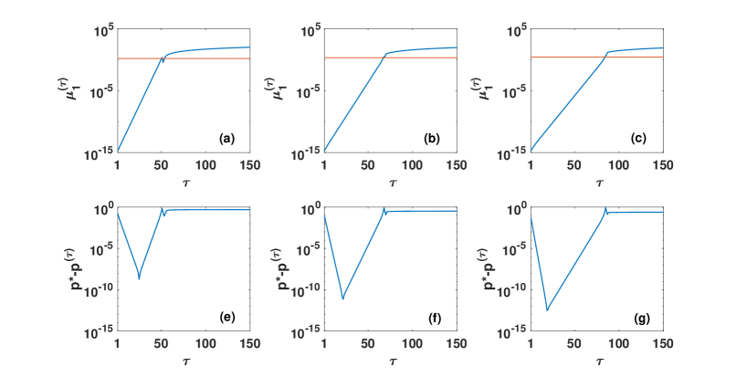
Figure 3: The RG flow for the Apollonian simplicial complex for $m=d-2$ is represented by plotting the numerically integrated values of $\mu_{1}^{(\tau)}$ and $p^{\star}-p^{\tau}$ versus $\tau$, where $p^{\star}=(d-1)/d$ (blue curves). The red curve indicates the constant value $\mu=d/2$, where Eq.(92) has a simple pole. Plots (a)-(e), (b)-(f) and (c)-(g) display the RG flow for dimension $d=2$, $d=3$ and $d=4$ respectively. In all the plots $\mu=10^{-15}$.

6.3 Case $m\leq d-3$

For deriving the RG flow for the case $m\leq d-3$ we can rewrite the RG Eqs.(71) in a simplified way with,

$$x_{\ell}=(1-\mu_{\ell})p_{\ell}.$$ (127)

We obtain a new set of RG equations relating the parameters $(\{x_{\ell}^{(\tau)}\},\{p_{\ell}^{(\tau)}\})$ at iteration $\tau$ of the RG transformation with the parameters $(\{x_{\ell}^{(\tau+1)}\},\{p_{\ell}^{(\tau+1)}\})$ at the next RG iteration. This set of equations is given by

$$x_{\ell}^{(\tau+1)}=\left[x_{\ell}^{(\tau)}+\left(x_{1}^{(\tau)}-\frac{(m+1)}{m+(d-m)x_{1}^{(\tau)}}\right)(d-m-2)^{\ell-1}\right]\left[p_{2}^{(\tau)}+\frac{d-m-1}{m+(d-m)x_{1}^{(\tau)}}\right]^{-1},$$

$$p_{\ell}^{(\tau+1)}=\left[p_{\ell+1}^{(\tau)}+\frac{(d-m-1)(d-m-2)^{\ell-1}}{m+(d-m)x_{1}^{(\tau)}}\right]\left[p_{2}^{(\tau)}+\frac{d-m-1}{m+(d-m)x_{1}^{(\tau)}}\right]^{-1},$$ (128)

with initial conditions $x_{\ell}^{(0)}=1-\mu$ and $p_{\ell}^{(0)}=1$. In order to find the solution of these equations we use the auxiliary variable $y_{1}^{(\tau)}$ given by

$${y}_{1}^{(\tau+1)}=p_{2}^{(\tau+1)}+\frac{d-m-1}{m+(d-m)x_{1}^{(\tau+1)}}.$$ (129)

The explicit solution of the RG equations (128) reads

$$p_{2}^{(\tau+1)}=\prod_{m=1}^{\tau}\frac{1}{y_{1}^{(m)}}+{(d-m-1)}\sum_{m=1}^{\tau}\frac{(d-m-2)^{\tau-m+1}}{m+(d-m)x^{(m)}}\prod_{m^{\prime}=m}^{\tau}\frac{1}{y_{1}^{(m^{\prime})}},$$

$${y}_{1}^{(\tau+1)}=p_{2}^{(\tau+1)}+\frac{d-m-1}{m+(d-m)x_{1}^{(\tau+1)}},$$

$$=\prod_{m=1}^{\tau}\frac{1}{y_{1}^{(m)}}+{(d-m-1)}\sum_{m=1}^{\tau}\frac{(d-m-2)^{\tau-m+1}}{m+(d-m)x^{(m)}}\prod_{m^{\prime}=m}^{\tau}\frac{1}{y_{1}^{(m^{\prime})}}+\frac{d-m-1}{m+(d-m)x_{1}^{(\tau+1)}},$$

$$x_{1}^{(\tau+1)}=x_{1}^{(1)}\prod_{m=1}^{\tau}\frac{1}{y_{1}^{(m)}}+\sum_{m=1}^{\tau}\left(x_{1}^{(m)}-\frac{(m+1)}{m+(d-m)x_{1}^{(m)}}\right)(d-m-2)^{\tau-m}\prod_{m^{\prime}=m}^{\tau}\frac{1}{y_{1}^{(m^{\prime})}}.$$

This solution shows that $p_{2}^{(\tau+1)},y_{1}^{(\tau+1)}$ and $x_{1}^{(\tau+1)}$ depend on the entire RG flow up to time $\tau$, i.e. on all the values of the parameters $p_{2}^{(\tau^{\prime})},y_{1}^{(\tau^{\prime})}$ and $x_{1}^{(\tau^{\prime})}$ with $\tau^{\prime}\leq\tau$. This solution therefore seems to indicate that in order to calculate the value of $x_{\ell}^{(\tau+1)}$ and $p_{\ell}^{(\tau+1)}$ the knowledge of the entire RG flow up to iteration $\tau$ is necessary. However, one can recover some Markovian recursive equations by introducing the additional auxiliary variables called $A^{(\tau)},B^{(\tau)}$ and $C^{(\tau)}$. The auxiliary variables $A^{(\tau)},B^{(\tau)}$ and $C^{(\tau)}$ are defined as

$$A^{(\tau)} = \prod_{m=1}^{\tau}\frac{1}{y_{1}^{(m)}},$$

$$B^{(\tau)} = {(d-m-1)}\sum_{m=1}^{\tau}\frac{(d-m-2)^{\tau-m+1}}{m+(d-m)x^{(m)}}\prod_{m^{\prime}=m}^{\tau}\frac{1}{y_{1}^{(m^{\prime})}}+\frac{d-m-1}{m+(d-m)x_{1}^{(\tau+1)}},$$

$$C^{(\tau)} = \sum_{m=1}^{\tau}\left(x_{1}^{(m)}-\frac{(m+1)}{m+(d-m)x_{1}^{(m)}}\right)(d-m-2)^{\tau-m}\prod_{m^{\prime}=m}^{\tau}\frac{1}{y_{1}^{(m^{\prime})}}.$$

The variables $y_{1}^{({\tau+1)}}$ and $x_{1}^{(\tau+1)}$ can be simply expressed in terms of $A^{(\tau)},B^{(\tau)}$ and $C^{(\tau)}$ by

$$y_{1}^{(\tau+1)} = A^{(\tau)}+B^{(\tau)},$$

$$x_{1}^{(\tau+1)} = (1-\mu)A^{(\tau)}+C^{(\tau)}.$$ (130)

The solution of the RG equations can be written as the following set of recursive equations for $A^{(\tau)},B^{(\tau)}$ and $C^{(\tau)}$

$$A^{(\tau+1)} = \frac{1}{y_{1}^{(\tau+1)}}A^{(\tau)},$$

$$B^{(\tau+1)} = \frac{d-m-2}{y_{1}^{(\tau+1)}}B^{(\tau)}+({d-m-1})\frac{1}{m+(d-m)x_{1}^{(\tau+2)}},$$

$$C^{(\tau+1)} = \frac{(d-m-2)}{y_{1}^{(\tau+1)}}C^{(\tau)}+\frac{1}{y_{1}^{(\tau+1)}}\left(x_{1}^{(\tau+1)}-\frac{(m+1)}{m+(d-m)x_{1}^{(\tau+1)}}\right).$$ (131)

This set of equations can be written as a closed set of equations for $A^{(\tau)},B^{(\tau)}$ and $C^{(\tau)}$ using Eq. (130), with initial conditions $A^{(0)}=1,B^{(0)}=(d-m-1)/(d-(d-m)\mu)),C^{(0)}=0$.

The fixed point of these RG equations at $\mu=0$ is

$$A^{\star}=0,$$

$$B^{\star}=\frac{d^{2}-(m+1)(d+1)}{d},$$

$$C^{\star}=1.$$ (132)

The Jacobian matrix of these RG equations has eigenvalues $\lambda_{1}>\lambda_{2}>\lambda_{3}$ given by

$$\lambda_{1}=\lambda=\frac{d^{2}-m(d+1)}{d^{2}-(m+1)(d+1)},$$

$$\lambda_{2}=\frac{d}{d^{2}-(m+1)(d+1)},$$

$$\lambda_{3}=0$$ (133)

with $\lambda_{1}>1$ and $\lambda_{2}<1$.

The right eigenvectors corresponding to these eigenvalues are

$${\bf u_{1}} = \frac{1}{c_{1}}\left(d^{2}+d-m(1-d+m),-d^{2},d^{3}-d^{2}+d-m(1-d+d^{2}+m)\right),$$

$${\bf u_{2}} = \left(1,0,0\right),$$

$${\bf u_{3}} = \frac{1}{c_{3}}\left(d^{3}-d^{2}-d+m(1-2d-d^{2}+m),d^{2},d^{2}-d+m(1-2d+m)\right),$$

where $c_{1}$ and $c_{3}$ are normalization constants. The left eigenvectors corresponding to these eigenvalues are

$${\bf v_{1}} = \frac{1}{d_{1}}\left(0,d^{2}-d+m(1-2d+m),-d^{2}\right),$$

$${\bf v_{2}} = \frac{1}{d_{2}}\left(-1,d-2-m,1\right),$$

$${\bf v_{3}} = \frac{1}{d_{3}}\left(0,d^{3}-d^{2}+d-m(1-d+d^{2}+m),d^{2}\right),$$

where $d_{1},d_{2},d_{3}$ are normalization constants. In order to solve Eqs.(131) we indicate with ${\bf X}^{(\tau)}$ the column vector

$${\bf X}^{(\tau)}=\left(A^{(\tau)},B^{(\tau)},C^{(\tau)}\right).$$ (134)

By linearizing Eqs.(131) near the fixed point ${\bf X}^{\star}$ given by

$${\bf X}^{\star}=\left(A^{\star},B^{\star},C^{\star}\right),$$ (135)

we obtain

$${\bf X}^{(\tau)}={\bf X}^{\star}+\sum_{m=1}^{3}\lambda_{m}^{\tau}{\bf v}_{m}\langle{{\bf u}_{m},{\bf X}^{(0)}-{\bf X}^{\star}}\rangle.$$ (136)

For the leading order term, we have

$${\bf X}^{(\tau)}={\bf X}^{\star}+\lambda_{1}^{\tau}{\bf v}_{1}\langle{{\bf u}_{1},{\bf X}^{(0)}-{\bf X}^{\star}}\rangle,$$ (137)

where the scalar product is,

$$\langle{{\bf u}_{1},{\bf X}^{(0)}-{\bf X}^{\star}}\rangle\propto\frac{\mu}{d-\mu(d-m)}.$$ (138)

We therefore have proved that for $\mu\ll 1$ we have,

$$\mu_{1}^{(\tau)}\propto\lambda^{\tau}\mu.$$ (139)

Using Eq. (94) it follows that for $m\leq d-3$ the spectral dimension $d_{S}$ decreases with increasing $m$ and is given by

$$d_{S}=2\frac{\ln d}{\ln\lambda}=2(\ln d)\left[\ln\left(\frac{d^{2}-m(d+1)}{d^{2}-(m+1)(d+1)}\right)\right]^{-1}.$$ (140)

Finally, we observe that in the limit $d\to\infty$ and $m\ll d$ the spectral dimension scales like

$$d_{S}\simeq(2\ln d)\left[d-m-\frac{3}{2}+O(1/d)\right].$$ (141)

The spectral dimension therefore grows faster than linearly with the topological dimension $d$.

7 General RG equations for the pseudo-fractal simplicial complex

7.1 The RG equations

In a $d$-dimensional pseudo-fractal simplicial complex at each iteration $n$ each $(d-1)$-simplex is glued to a new $d$-dimensional simplex. The difference with the algorithm generating the Apollonian simplicial complexes is that in the case of the Apollonian simplicial complex at each iteration $n$ only the $(d-1)$-simplices of the last generation are glued to a new $d$-dimensional simplex. Given the structure of the pseudo-fractal simplicial complex and its relation to the Apollonian simplicial complex, which was already noted in Ref.[28], the general RG equations for the pseudo-fractal simplicial complex can be easily derived from those for the Apollonian simplicial complex. In fact it is sufficient to observe that in the pseudo-fractal simplicial complex each simplex of type $\ell$ receives the sum of the contributions coming from the integration of the Gaussian variables associated to the $d$-simplices added at the last generation. The RG equations for $m\leq d-2$ are therefore given by

$$(1-\mu_{\ell}^{\prime})p_{\ell}^{\prime}=\left[(1-\mu_{\ell+1})p_{\ell+1}+\left((1-\mu_{1})-\frac{(m+1)}{d-(d-m)\mu_{1}}\right)\sum_{\ell^{\prime}=0}^{\ell-1}(d-m-2)^{\ell^{\prime}}\right]$$

$$\times\left[p_{2}+\frac{(d-m-1)}{d-(d-m)\mu_{1})}\right]^{-1},$$

$$p^{\prime}_{\ell}=\left[p_{\ell+1}+\frac{(d-m-1)}{d-(d-m)\mu_{1}}\sum_{\ell^{\prime}=0}^{\ell-1}(d-m-2)^{\ell^{\prime}}\right]\left[p_{2}+\frac{(d-m-1)}{d-(d-m)\mu_{1}}\right]^{-1},$$ (142)

for all $\ell\geq 1$, with initial conditions $(\mu_{\ell},p_{\ell})=(\mu,1)$ with $\mu\ll 1$ for all $\ell\geq 1$. For $m=d-1$ every $m$-simplex of type $\ell$ is connected to a $d$-simplex of generation $n$ and the RG equations for $m=d-1$ and $\ell\geq 1$ read

$$p_{\ell}=p_{1}=1$$ (143)

and

$$(1-\mu_{\ell}^{\prime})=(1-\mu_{\ell+1})+\left[(1-\mu_{1})-\frac{d}{d-\mu_{1}}\right]$$ (144)

with initial conditions $(\mu_{\ell},p_{\ell})=(\mu,1)$ with $\mu\ll 1$ for all $\ell\geq 1$.

7.2 The free-energy density and the spectral dimension

The free energy is given by Eq. (60). By using a procedure similar to the one used to derive the corresponding expression for the Apollonian simplicial complex we easily find for $m\leq d-2$

$$g(\bm{\omega})=\frac{{\mathcal{N}}_{n}}{2N_{n}}\ln G(\mu_{1})+\frac{N_{n-1}}{2N_{n}}\ln\left[p_{2}+\frac{d-m-1}{d-(d-m)\mu_{1})}\right]+c,$$ (145)

where $c$ is a constant. Given this expression for $g(\bm{\omega})$, the free energy density $f$ obtained from Eq. (60) reads

$$f\simeq\sum_{\tau=0}^{\infty}\frac{g(R^{(\tau)}\bm{\omega})}{(d+1)^{\tau}}$$

$$\simeq\sum_{\tau=0}^{\infty}\frac{1}{(d+1)^{\tau}}\left\{\frac{d}{2(d+1)}\ln G\left(\mu_{1}^{(\tau)}\right)+\frac{1}{2(d+1)}\ln\left[p_{2}^{(\tau)}+\frac{d-m-1}{d-(d-m)\mu_{1}^{(\tau)}}\right]\right\}.$$

For the pseudo-fractal complex, we expect to find a relevant repulsive fixed point at $(\mu^{\star},p_{2}^{\star})=(0,p^{\star})$. Under this hypothesis the RG flow is described by

$$\mu_{1}^{(\tau)}\simeq\mu\lambda^{\tau}$$

$$p_{2}^{(\tau)}\simeq p^{\star}+\lambda^{\tau}(1-p^{\star})$$ (146)

close to the relevant fixed point, where $\lambda>1$ is the largest eigenvalue of the linearized RG equations close to the relevant fixed point. Using Eq. (45), the spectral density $\bar{\rho}(\mu)$ can be expressed as

$$\bar{\rho}(\mu)\simeq\frac{2}{\pi}\mbox{Im}\sum_{\tau=0}^{\infty}\frac{1}{(d+1)^{\tau}}\frac{\partial g(\mu_{1}^{(\tau)},p_{2}^{\tau})}{\partial\mu}$$

$$\simeq\frac{2}{\pi}\mbox{Im}\sum_{\tau=0}^{\infty}\frac{\lambda^{\tau}}{(d+1)^{\tau}}\frac{d}{2(d+1)}\left[{{d-1}\choose{m}}\frac{1}{d-(d-m)\mu_{1}^{(\tau)}}+{{d-1}\choose{m-1}}\frac{1}{\mu_{1}^{(\tau)}}\right]$$

$$+\frac{2}{\pi}\mbox{Im}\sum_{\tau=0}^{\infty}\frac{\lambda^{\tau}}{(d+1)^{\tau}}\frac{d-m}{2(d+1)}y\left[\left(p_{2}^{(\tau)}\left[d-(d-m)\mu_{1}^{(\tau)}\right]+y\right)\left(d-(d-m)\mu_{1}^{(\tau)}\right)\right]^{-1},$$ (147)

where $y=d-m-1$. In the pseudo-fractal simplicial complex, the spectrum of the up-Laplacian of order $m$ acquires a delta peak at $\mu=0$ as well. This corresponds to the finite density of zero eigenvalues of the up-Laplacian, i.e.

$$\bar{\rho}(\mu)=\bar{\rho}(0)\hat{\delta}(\mu)+{\rho}(\mu)$$ (148)

where $\bar{\rho}(0)$ given by

$$\bar{\rho}(0)=\frac{d}{d+1}{{d-1}\choose{m-1}}\frac{1}{1-1/(d+1)}.$$ (149)

and the regular part of the spectrum is given by

$${\rho}(\mu)\simeq\frac{2}{\pi}\mbox{Im}\sum_{\tau=0}^{\infty}\frac{\lambda^{\tau}}{(d+1)^{\tau}}\frac{d}{2(d+1)}\left[{{d-1}\choose{m}}\frac{1}{d-(d-m)\mu_{1}^{(\tau)}}\right]$$

$$+\frac{2}{\pi}\mbox{Im}\sum_{\tau=0}^{\infty}\frac{\lambda^{\tau}}{(d+1)^{\tau}}\frac{d-m}{2(d+1)}y\left[\left(p_{2}^{(\tau)}\left[d-(d-m)\mu_{1}^{(\tau)}\right]+y\right)\left(d-(d-m)\mu_{1}^{(\tau)}\right)\right]^{-1}.$$ (150)

By approximating this expression with an integral over $\tau$ and by changing the variable of this integral to $z=\lambda^{\tau}$ we can approximate $\rho(\mu)$ by using the residue theorem at the pole $\mu_{1}^{(\tau)}=z\mu=d/(d-m)$, obtaining the asymptotic scaling

$${\rho}(\mu) \simeq C\mu^{d_{S}/2-1}.$$ (151)

The spectral dimension $d_{S}$ is then given by

$$d_{S}=2\frac{\ln(d+1)}{\ln\lambda}.$$ (152)

For $m=d-1$ the Gaussian fields are not rescaled and $g(\bm{\omega})$ is given by

$$g(\bm{\omega})=\frac{{\mathcal{N}}_{n}}{2N_{n}}\ln G(\mu_{1})+c,$$ (153)

where $c$ is a constant. Using this expression and Eq. (60) we can approximate the free energy $f$ by

$$f \simeq \sum_{\tau=0}^{\infty}\frac{g(R^{(\tau)}\bm{\omega})}{(d+1)^{\tau}}=\sum_{\tau=0}^{\infty}\frac{1}{(d+1)^{\tau}}\left\{\frac{d}{2(d+1)}\ln G\left(\mu_{1}^{(\tau)}\right)\right\},$$ (154)

with $G(\mu_{1})$ given by Eq.(69). Using Eq. (45), we can deduce that the spectral density $\bar{\rho}(\mu)$ is given by

$$\rho(\mu)\simeq\frac{2}{\pi}\mbox{Im}\sum_{\tau=0}^{\infty}\frac{1}{(d+1)^{\tau}}\frac{\partial g(\mu_{1}^{(\tau)},p_{2}^{\tau})}{\partial\mu}$$

$$\simeq\frac{2}{\pi}\mbox{Im}\sum_{\tau=0}^{\infty}\frac{\lambda^{\tau}}{(d+1)^{\tau}}\frac{d}{2(d+1)}\left[{{d-1}\choose{m}}\frac{1}{d-(d-m)\mu_{1}^{(\tau)}}+{{d-1}\choose{m-1}}\frac{1}{\mu_{1}^{(\tau)}}\right].$$ (155)

8 RG flow for the pseudo-fractal simplicial complex

In this section we will treat the RG flow for the pseudo-fractal simplicial complex. We consider the cases $m=d-1,m=d-2,m=d-3$ and $m<d-3$.

8.1 Case $m=d-1$

The RG equations for $m=d-1$ are given by Eqs.(144), which can be used to derive the following recursive equation for $\mu_{1}$,

$$\mu_{1}^{\prime} = \mu_{1}-\left[(1-\mu_{1})-\frac{d}{d-\mu_{1}}\right],$$ (156)

with initial condition $\mu_{1}=\mu.$ The fixed points of this equations are

$$\mu_{1}^{\star}=0,$$ (157)

$$\mu_{1}^{\star}=d+1.$$ (158)

At the fixed point at $\mu^{\star}=0$ the recursive equation Eqs.(156) has eigenvalue

$$\lambda=2+\frac{1}{d}>1,$$ (159)

so $\mu^{\star}=0$ is a repulsive fixed point. The RG flow starts from $\mu_{1}=\mu\ll 1$ and runs away from $\mu^{\star}=0$ according to

$$\mu^{(\tau)}=\mu\lambda^{\tau}.$$ (160)

In doing so, the RG flow approaches the singularity of Eq.(156) at $\mu_{1}=d$ and the linearised RG flow described by Eq. (160) is not longer valid. Therefore the RG flow changes its trend, in some cases even changing sign. This scenario is apparent from Figure 4 were the absolute values of $\mu_{1}^{(\tau)}$ (indicating the value of the parameter $\mu_{1}$ at iteration $\tau$ of the RG transformation) are plotted versus $\tau$ This is a situation analogous to the case $m=d-2$ for the Apollonian simplicial complexes, where the RG flow changes trends very close to the pole in Eq.(155). In this case $\lambda$ cannot be used to give a good estimation of the spectral dimension $d_{S}$.

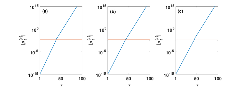
Figure 4: The RG flow of the pseudo-fractal simplicial complex for $m=d-1$ is represented by plotting the numerically integrated values of $|\mu_{1}^{(\tau)}|$ versus $\tau$ (blue curves). The red curves indicate the constant value $\mu_{1}=d$ where Eq.(155) has a simple pole. Plots (a), (b) and (c) display RG flow for dimension $d=2$, $d=3$ and $d=4$ respectively. In all the plots $\mu=10^{-15}$.

8.2 Case $m=d-2$

For $m=d-2$ the RG Eqs.(142) for the pseudo-fractal simplicial complex greatly simplify. We have

$$\mu_{\ell}=\mu_{1}$$ (161)

for $\ell\geq 1$ and

$$p_{\ell}=p$$

for all $\ell\geq 2$. The resulting RG equations are

$$(1-\mu_{1}^{\prime})=\left[2(1-\mu_{1})-\frac{d-1}{d-2\mu_{1}}\right]\left[1+\frac{1}{d-2\mu_{1}}\right]^{-1},$$

$$p^{\prime}=1,$$ (163)

with initial conditions $(\mu_{\ell},p_{\ell})=(\mu,1)$ with $\mu\ll 1$ for all $\ell\geq 1$. The fixed point is $(\mu^{\star},p^{\star})=(0,1)$. The eigenvalue of this system of equations is

$$\lambda=2.$$ (164)

The fixed point is $\mu^{\star}_{1}=0$ and $p^{\star}=1$ with eigenvalue $\lambda=2$. Using Eq.(152) we can predict the spectral dimension

$$d_{S}=2\frac{\ln(d+1)}{\ln\lambda}=2\frac{\ln(d+1)}{\ln 2}.$$ (165)

8.3 Case $m=d-3$

In the case $m=d-3$ the RG Eqs.(142) can be expressed in terms of the variables $x_{\ell}$ as defined in Eq. (127). Using $x_{\ell}^{(\tau)}$ and $p_{\ell}^{(\tau)}$ for indicating the parameter values at iteration $\tau$, by performing the sum over $\ell^{\prime}$, the Eqs. (142) for $m=d-3$ can be written as

$$x_{\ell}^{(\tau+1)}=\left[x_{\ell+1}^{(\tau)}+\left(x_{1}^{(\tau)}-\frac{d-2}{m+3x_{1}^{(\tau)}}\right)\ell\right]\left[p_{2}^{(\tau)}+\frac{d-m-1}{m+3x_{1}^{(\tau)}}\right]^{-1},$$

$$p_{\ell}^{(\tau+1)}=\left[p_{\ell+1}^{(\tau)}+\frac{(d-m-1)\ell}{m+3x_{1}^{(\tau)}}\right]\left[p_{2}^{(\tau)}+\frac{d-m-1}{m+3x_{1}^{(\tau)}}\right]^{-1},$$ (166)

with initial conditions $x_{\ell}^{(0)}=1-\mu$ and $p_{\ell}^{(0)}=1$. Equations (166) can be solved in terms of the auxiliary variable

$$y_{1}^{(\tau+1)} = p_{2}^{(\tau+1)}+\frac{2}{m+3x_{1}^{(\tau+1)}},$$ (167)

and we obtain

$$x_{1}^{(\tau+1)}=(1-\mu)\prod_{m=1}^{\tau}\frac{1}{y_{1}^{(m)}}+\sum_{m=1}^{\tau}\left(x_{1}^{(m)}-\frac{d-2}{m+3x_{1}^{(m)}}\right)(\tau+1-m)\prod_{m^{\prime}=m}^{\tau}\frac{1}{y^{(m^{\prime})}},$$

$$p^{(\tau+1)}_{2}=\prod_{m=1}^{\tau}\frac{1}{y_{1}^{(m)}}+({d-m-1})\sum_{m=1}^{\tau}\frac{1}{m+3x_{1}^{(m)}}(\tau+2-m)\prod_{m^{\prime}=m}^{\tau}\frac{1}{y^{(m^{\prime})}}.$$ (168)

Also in the pseudo-fractal case these non-Markovian equations can be turned to Markovian iterative relations by expressing the variable at iteration $\tau+1$ exclusively in terms of the variable at iteration $\tau$. This is achieved by introducing the auxiliary variables $A^{(\tau)},B^{(\tau)},C^{(\tau)},D^{(\tau)}$ and $E^{(\tau)}$ defined as

$$A^{(\tau)} = \prod_{m=1}^{\tau}\frac{1}{y_{1}^{(m)}},$$

$$B^{(\tau)} = \sum_{m=1}^{\tau}\frac{2}{d+3x_{1}^{(m)}}(\tau+2-m)\prod_{m^{\prime}=m}^{\tau}\frac{1}{y^{(m^{\prime})}},$$

$$C^{(\tau)} = \sum_{m=1}^{\tau}\left(x_{1}^{(m)}-\frac{d-2}{m+3x_{1}^{(m)}}\right)(\tau+1-m)\prod_{m^{\prime}=m}^{\tau}\frac{1}{y^{(m^{\prime})}},$$

$$D^{(\tau)} = \sum_{m=1}^{\tau}\left(x_{1}^{(m)}-\frac{d-2}{m+3x_{1}^{(m)}}\right)\prod_{m^{\prime}=m}^{\tau}\frac{1}{y^{(m^{\prime})}},$$

$$E^{(\tau)} = \sum_{m=1}^{\tau}\frac{2}{m+3x_{1}^{(m)}}\prod_{m^{\prime}=m}^{\tau}\frac{1}{y^{(m^{\prime})}}.$$ (169)

These auxiliary variables are related to $y_{1}^{(\tau)}$ and $x_{1}^{(\tau)}$ by

$$y_{1}^{(\tau+1)} = A^{(\tau)}+B^{(\tau)}+\frac{2}{m+3x_{1}^{(\tau+1)}},$$

$$x_{1}^{(\tau+1)} = (1-\mu)A^{(\tau)}+C^{(\tau)}.$$ (170)

The recursive Markovian RG equations for the case $m=d-3$ read

$$x_{1}^{(\tau+1)} = (1-\mu)A^{(\tau)}+C^{(\tau)},$$

$$y_{1}^{(\tau+1)} = A^{(\tau)}+B^{(\tau)}+\frac{2}{m+3[(1-\mu)A^{(\tau)}+C^{(\tau)}]},$$

$$A^{(\tau+1)} = \frac{1}{y_{1}^{(\tau+1)}}A^{(\tau)},$$

$$B^{(\tau+1)} = \frac{1}{y_{1}^{(\tau+1)}}\left[B^{(\tau)}+E^{(\tau)}+\frac{4}{m+3x_{1}^{(\tau+1)}}\right],$$

$$C^{(\tau+1)} = \frac{1}{y_{1}^{(\tau+1)}}\left[C^{(\tau)}+D^{(\tau)}+\left(x_{1}^{(\tau+1)}-\frac{d-2}{m+3x_{1}^{(\tau+1)}}\right)\right],$$

$$D^{(\tau+1)} = \frac{1}{y_{1}^{(\tau+1)}}\left[D^{(\tau)}+\left(x_{1}^{(\tau+1)}-\frac{d-2}{m+3x_{1}^{(\tau+1)}}\right)\right],$$

$$E^{(\tau+1)} = \frac{1}{y_{1}^{(\tau+1)}}\left[E^{(\tau)}+\frac{2}{m+3x_{1}^{(\tau+1)}}\right],$$ (171)

with initial conditions $A^{(1)},B^{(1)},C^{(1)},D^{(1)}$ and $E^{(1)}$, which can be found by inserting $x_{1}^{(0)}=1-\mu$ and $y_{1}^{(0)}=1+\frac{2}{m+3(1-\mu)}$ in Eqs. (169) and (170).

The relevant fixed point of these equations is

$$A^{\star} = 0,$$

$$B^{\star} = \frac{1}{d}\left(d-1+\sqrt{1+2d}\right),$$

$$C^{\star} = 1,$$

$$D^{\star} = \frac{1}{d}\left(-1+{\sqrt{1+2d}}\right),$$

$$E^{\star} = \frac{1}{d}\left(-1+{\sqrt{1+2d}}\right).$$

Close to this fixed point, the RG equations (171) have the relevant eigenvalue

$$\lambda=[1+d+\sqrt{1+2d}]^{-2}\hat{x},$$ (173)

where $\hat{x}$ is the largest positive real root of the equation

$$-d^{6}-2d^{5}\sqrt{2d+1}-4d^{5}-2d^{4}\sqrt{2d+1}-2d^{4}$$

$$+\left(4d^{4}+5d^{3}\sqrt{2d+1}+10d^{3}+5d^{2}\sqrt{2d+1}+5d^{2}\right)x$$

$$+\left(-4d^{2}-3d\sqrt{2d+1}-6d-3\sqrt{2d+1}-3\right)x^{2}+x^{3}=0$$ (174)

Using Eq.(152) we obtain that the spectral dimension $d_{S}$ is therefore given by

$$d_{S}=2\frac{\ln(d+1)}{\ln\lambda}.$$ (175)

8.4 Case $m<d-3$

In this paragraph we study the RG flow for the pseudo-fractal simplicial complex for $m<d-3$. By expressing Eqs. (142) in terms of the variables $x_{\ell}^{(\tau)}$ defined in Eq. (127) and the variables $p_{\ell}^{(\tau)}$ calculated at iteration $\tau$, we obtain the recursive equations

$$x_{\ell}^{(\tau+1)}=\left[x_{\ell+1}^{(\tau)}+\left(x_{1}^{(\tau)}-\frac{(m+1)}{m+(d-m)x_{1}^{(\tau)}}\right)\frac{[(d-m-2)^{\ell}-1]}{d-m-3}\right]\left[p_{2}^{(\tau)}+\frac{d-m-1}{m+(d-m)x_{1}^{(\tau)}}\right]^{-1},$$

$$p^{(\tau+1)}_{\ell}=\left[p_{\ell+1}^{(\tau)}+\frac{(d-m-1)}{m+(d-m)x_{1}^{(\tau)}}\frac{[(d-m-2)^{\ell}-1]}{d-m-3}\right]\left[p_{2}^{(\tau)}+\frac{d-m-1}{m+(d-m)x_{1}^{(\tau)}}\right]^{-1},$$ (176)

with initial conditions $x_{\ell}^{(0)}=1-\mu$ and $p_{\ell}^{(0)}=1$. These equations can be solved in terms of the variables $y_{1}^{(\tau)}$ defined as

$${y}_{1}^{(\tau)}=p_{2}^{(\tau)}+\frac{(d-m-1)}{m+(d-m)x_{1}^{(\tau)}}.$$ (177)

In particular the solution of Eqs. (176) is given by

$$p_{2}^{(\tau+1)} = \prod_{m=1}^{\tau}\frac{1}{y_{1}^{(m)}}+\frac{(d-m-1)}{(d-m-3)}\sum_{m=1}^{\tau}\frac{[(d-m-2)^{\tau-m+2}-1]}{m+(d-m)x^{(m)}}\prod_{m^{\prime}=m}^{\tau}\frac{1}{y_{1}^{(m^{\prime})}},$$

$$y_{1}^{(\tau+1)} = p_{2}^{(\tau+1)}+\frac{(d-m-1)}{m+(d-m)x_{1}^{(\tau+1)}}$$

$$= \prod_{m=1}^{\tau}\frac{1}{y_{1}^{(m)}}+\frac{(d-m-1)}{(d-m-3)}\sum_{m=1}^{\tau}\frac{[(d-m-2)^{\tau-m+2}-1]}{m+(d-m)x^{(m)}}\prod_{m^{\prime}=m}^{\tau}\frac{1}{y_{1}^{(m^{\prime})}}$$

$$+\frac{(d-m-1)}{m+(d-m)x_{1}^{(\tau+1)}},$$

$$x_{1}^{(\tau+1)} = x_{1}^{(1)}\prod_{m=1}^{\tau}\frac{1}{y_{1}^{(m)}}+\frac{1}{d-m-3}\sum_{m=1}^{\tau}\left(x_{1}^{(m)}-\frac{m+1}{m+(d-m)x_{1}^{(m)}}\right)$$ (178)

$$\times[(d-m-2)^{\tau+1-m}-1]\prod_{m^{\prime}=m}^{\tau}\frac{1}{y_{1}^{(m^{\prime})}}.$$

In order to turn this system of equations into a Markovian system of equations, we again express the variables at iteration $\tau+1$ only in terms of variables at iteration $\tau$. We then have

$$y_{1}^{(\tau+1)} = A^{(\tau)}+B^{(\tau)}-D^{(\tau)}+\frac{(d-m-1)}{m+(d-m)x_{1}^{(\tau+1)}},$$

$$x_{1}^{(\tau+1)} = (1-\mu)A^{(\tau)}+C^{(\tau)}-E^{(\tau)}$$

with $A^{(\tau)},B^{(\tau)},C^{(\tau)},D^{(\tau)},E^{(\tau)}$ given by

$$A^{(\tau)} = \prod_{m=1}^{\tau}\frac{1}{y_{1}^{(m)}},$$

$$B^{(\tau)} = =\frac{(d-m-1)}{(d-m-3)}\sum_{m=1}^{\tau}\frac{(d-m-2)^{\tau-m+2}}{m+(d-m)x^{(m)}}\prod_{m^{\prime}=m}^{\tau}\frac{1}{y_{1}^{(m^{\prime})}},$$

$$C^{(\tau)} = \frac{1}{d-m-3}\sum_{m=1}^{\tau}\left(x_{1}^{(m)}-\frac{(m+1)}{m+(d-m)x_{1}^{(m)}}\right)(d-m-2)^{\tau+1-m}\prod_{m^{\prime}=m}^{\tau}\frac{1}{y_{1}^{(m^{\prime})}},$$

$$D^{(\tau)} = \frac{(d-m-1)}{(d-m-3)}\sum_{m=1}^{\tau}\frac{1}{m+(d-m)x^{(m)}}\prod_{m^{\prime}=m}^{\tau}\frac{1}{y_{1}^{(m^{\prime})}},$$

$$E^{(\tau)} = \frac{1}{d-m-3}\sum_{m=1}^{\tau}\left(x_{1}^{(m)}-\frac{(m+1)}{m+(d-m)x_{1}^{(m)}}\right)\prod_{m^{\prime}=m}^{\tau}\frac{1}{y_{1}^{(m^{\prime})}}.$$ (179)

The RG flow can therefore be cast in a set of recursive equations for $A^{(\tau)},B^{(\tau)},C^{(\tau)},D^{(\tau)}$ and $E^{(\tau)}$ given by

$$y_{1}^{(\tau+1)} = A^{(\tau)}+B^{(\tau)}-D^{(\tau)}+\frac{d-m-1}{m+(d-m)[(1-\mu)A^{(\tau)}+C^{(\tau)}-E^{(\tau)}]},$$

$$x_{1}^{(\tau+1)} = (1-\mu)A^{(\tau)}+C^{(\tau)}-E^{(\tau)},$$

$$A^{(\tau+1)} = \frac{1}{y_{1}^{(\tau+1)}}A^{(\tau)},$$

$$B^{(\tau+1)} = \frac{d-m-2}{y_{1}^{(\tau+1)}}B^{(\tau)}+\frac{(d-m-1)(d-m-2)^{2}}{(d-m-3)}\frac{1}{y_{1}^{(\tau+1)}[m+(d-m))x_{1}^{(\tau+1)}]},$$

$$C^{(\tau+1)} = \frac{(d-m-2)}{y_{1}^{(\tau+1)}}C^{(\tau)}+\frac{(d-m-2)}{(d-m-3)}\frac{1}{y_{1}^{(\tau+1)}}\left(x_{1}^{(\tau+1)}-\frac{(m+1)}{m+(d-m)x_{1}^{(\tau+1)}}\right),$$

$$D^{(\tau+1)} = \frac{1}{y_{1}^{(\tau+1)}}D^{(\tau)}+\frac{(d-m-1)}{(d-m-3)}\frac{1}{y_{1}^{(\tau+1)}[m+(d-m)x_{1}^{(\tau+1)}]},$$

$$E^{(\tau+1)} = \frac{1}{y_{1}^{(\tau+1)}}E^{(\tau)}+\frac{1}{(d-m-3)}\frac{1}{y_{1}^{(\tau+1)}}\left(x_{1}^{(\tau+1)}-\frac{(m+1)}{m+(d-m)x_{1}^{(\tau+1)}}\right),$$ (180)

with initial conditions $A^{(1)},B^{(1)},C^{(1)},D^{(1)},E^{(1)}$ which can be found by inserting $x_{1}^{(0)}=1-\mu$ and $y_{1}^{(0)}=[1+\frac{d-m-1}{d-m\mu)}]$ in Eq. (179).

By extracting the leading eigenvalue $\lambda$ close to the relevant fixed point at $\mu^{\star}=0$ and using Eq. (152) we can deduce the values of the spectral dimension $d_{S}$ (see Table 2).

Here we make an additional useful observation. As is true for the specific case $m=0$ and $d>3$ (see Ref.[28]) and in the more general case investigated here with $m<d-3$, we observe that the RG Eqs.(176) of the pseudo-fractal simplicial complex have the same leading term of the RG Eqs.(128) valid for the Apollonian simplicial complex with $m<d-3$. Therefore the leading eigenvalue $\lambda$ of the Eqs.(176) is given by

$$\lambda=\frac{{d^{2}}-m(d+1)}{d^{2}-(m+1)(d+1)}+\mathcal{O}(d^{-1}).$$ (181)

It follows that for $d\gg 1$ and $m$ finite, the spectral dimension $d_{S}$ obeys the asymptotic scaling

$$d_{S}\simeq 2(d-m)\log(d+1)+{\mathcal{O}}(\log(d)),$$ (182)

i.e. it grows faster than linearly with $d$.

9 Main results and comparison to numerical results

9.1 Higher-order spectral dimensions of Apollonian and pseudo-fractal simplicial complexes

Table 1: Numerical values for the spectral dimension $d_{S}$ of the $m$-up-Laplacian (with $m\leq d-3$) of the $d$-dimensional Apollonian simplicial complexes up to dimension $d=9$. The values of $d_{S}$ are rounded at the sixth significant figure.

• $d$/$m$	$d=2$	$d=3$	$d=4$	$d=5$	$d=6$	$d=7$	$d=8$	$d=9$
  $m=d-3$	-	3.73813	4.5742	5.19979	5.70072	6.11932	6.47949	6.79596
  $m=d-4$	-	-	7.39962	8.48212	9.35664	10.0913	10.7253	11.2833
  $m=d-5$	-	-	-	11.729	12.9719	14.0179	14.9217	15.7178
  $m=d-6$	-	-	-	-	16.5732	17.9293	19.1017	20.1346
  $m=d-7$	-	-	-	-	-	21.8337	23.2741	24.5434
  $m=d-8$	-	-	-	-	-	-	27.4423	28.9478
  $m=d-9$	-	-	-	-	-	-	-	33.3496

Table 2: Numerical values for the spectral dimension $d_{S}$ of the $m$-up-Laplacian (with $m\leq d-2$) of the $d$-dimensional pseudo-fractal simplicial complexes up to dimension $d=9$. The values of $d_{S}$ are rounded at the sixth significant figure.

• $d$/$m$	$d=2$	$d=3$	$d=4$	$d=5$	$d=6$	$d=7$	$d=8$	$d=9$
  $m=d-2$	3.16993	4.0	4.64386	5.16993	5.61471	6.0	6.33985	6.64386
  $m=d-3$	-	5.31562	5.86924	6.28083	6.60535	6.87191	7.0975	7.29281
  $m=d-4$	-	-	8.37610	8.99732	9.49705	9.91547	10.276	10.5934
  $m=d-5$	-	-	-	12.7140	13.7232	14.4689	15.057	15.5463
  $m=d-6$	-	-	-	-	17.3048	18.5860	19.5562	20.3283
  $m=d-7$	-	-	-	-	-	22.2618	23.7403	24.897
  $m=d-8$	-	-	-	-	-	-	27.5667	29.1935
  $m=d-9$	-	-	-	-	-	-	-	33.1841

In the preceding paragraphs we have derived the equations from which we can deduce the spectral dimensions $d_{S}$ of the up-Laplacians of order $m$ of the Apollonian and pseudo-fractal simplicial complexes. The only exceptions are the case $m=d-2$ for the Apollonian network and the case $m=d-1$ for the pseudo-fractal network. The predicted values for the spectral dimensions $d_{S}$ for $d$-dimensional Apollonian ($m\leq d-3$) and pseudo-fractal simplicial complexes ($m\leq d-2$ ) up to dimension $d=9$ are shown in Table 1 and Table 2 respectively. In Figure 5 and Figure 6) we compare the spectra obtained by numerical diagonalization of the higher-order up-Laplacians for Apollonian and pseudo-fractal simplicial complexes of dimension $d=3$ and $d=4$. We find a very good agreement with our exact analytical results. In addition we can fit the numerical data finding the spectral dimensions for the case $m=d-1$ of the Apollonian simplicial complex and the case $m=d-2$ of the pseudo-fractal simplicial complex.

From our RG calculations of the spectrum of higher-order up-Laplacians of Apollonian simplicial complexes and pseudo-fractal simplicial complexes and its numerical validation we draw the following main conclusions:

• Higher-order up-Laplacians of order $m$ on Apollonian and pseudo-fractal simplicial complexes display a finite spectral dimension with the only exception of the case of $m=d-1$ for the Apollonian simplicial complex. A single simplicial complex generated by the above-mentioned models is therefore not just characterized by a single spectral dimension but by multiple spectral dimensions corresponding to different orders $m$.

• The analytical prediction of the spectrum of the $m$-order up-Laplacian on $d$-dimensional Apollonian and pseudo-fractal simplicial complexes shows that the spectral dimension $d_{S}$ decreases with increasing $m$ as long as $m\leq d-3$ for the Apollonian simplicial complexes and as long as $m\leq d-2$ for the pseudo-fractal simplicial complex.

• The symmetries of the simplicial complex do not only induce degenerate eigenvalues for the graph Laplacian [28] but also for their higher-dimensional counterparts. Indeed, from our numerical results (Figures 5) and 6)) we observe that the higher-order up-Laplacian have several eigenvalues that are highly degenerate.

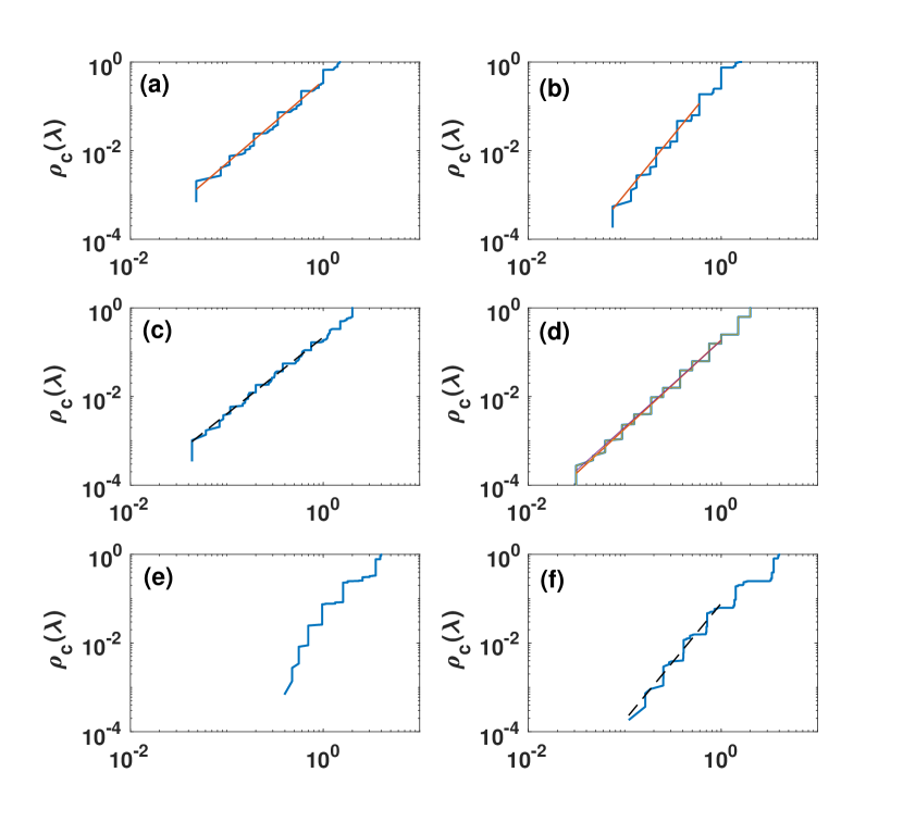
Figure 5: The cumulative density of eigenvalues $\rho_{c}(\lambda)$ of the up-Laplacians of order $m$ is shown in solid lines for the Apollonian and the pseudo-fractal simplicial complex of dimension $d=3$. Panels (a), (c) and (e) display results (blue lines) for the up-Laplacian of order $m$ of the Apollonian simplicial complex with respectively $m=0,1,2$. Panels (b), (d) and (f) display results (blue lines) for the up-Laplacian of order $m$ of the pseudo-fractal simplicial complex with respectively $m=0,1,2$. The theoretically predicted spectral dimensions are shown with red lines. Dashed black lines indicate power-law fits.

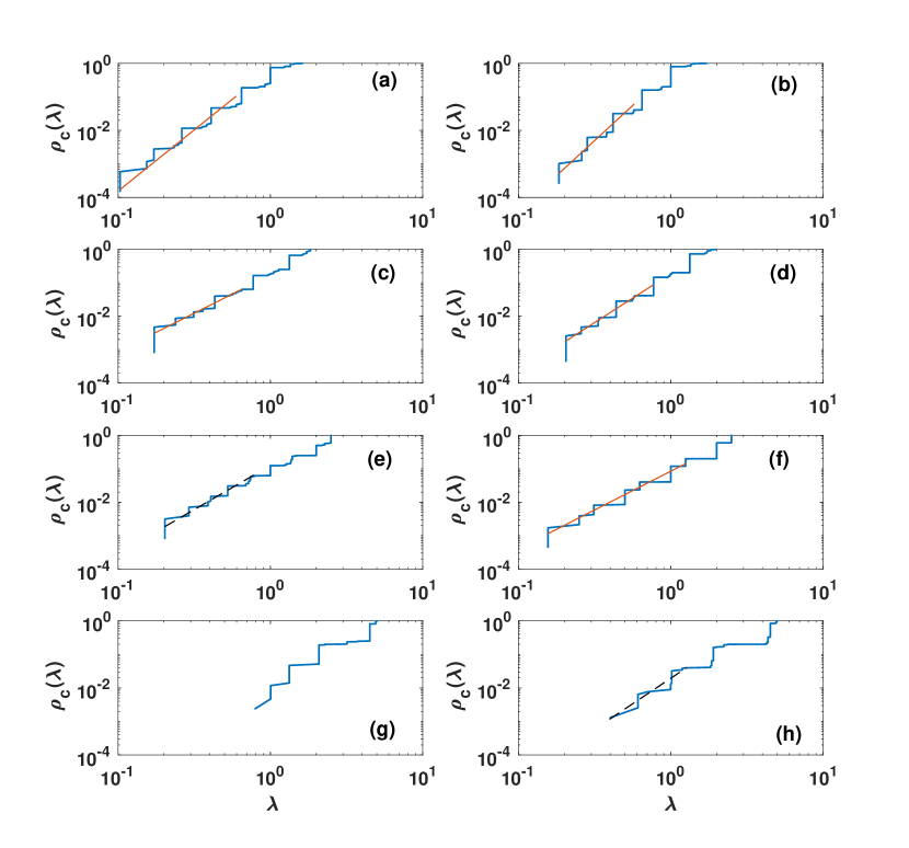
Figure 6: The cumulative density of eigenvalues $\rho_{c}(\lambda)$ of the up-Laplacians of order $m$ is shown in solid lines for the Apollonian and the pseudo-fractal simplicial complex of dimension $d=4$. Panels (a), (c), (e) and (g) display results (blue lines) for the up-Laplacian of order $m$ of the Apollonian simplicial complex with respectively $m=0,1,2,3$. Panels (b), (d), (f) and (h) display results (blue lines) for the up-Laplacian of order $m$ of the pseudo-fractal simplicial complex with respectively $m=0,1,2,3$. The theoretically predicted spectral dimensions are shown with red lines. Dashed black lines indicate power-law fits.

10 Conclusions

Higher-order Laplacians are important topological objects that generalize graph Laplacians and extend the notion of diffusion to higher dimension. Here we show that two non-amenable simplicial complex models (the Apollonian simplicial complex, the pseudo-fractal simplicial complex) display finite higher-order spectral dimensions $d_{S}$. We observe that a single simplicial complex can be characterized by a set of spectral dimensions corresponding to the spectrum of the up-Laplacians of different order $m$. We have used renormalization group methods applied to a Gaussian model to predict the higher-order spectral dimension $d_{S}$ of up-Laplacians of order $m$ of the Apollonian simplicial complex and the pseudo-fractal simplicial complex of arbitrary dimension $d$. With our RG approach it is possible to analytically calculate the spectral dimension $d_{S}$ for order $m\leq d-3$ for the Apollonian simplicial complexes and for order $m\leq d-2$ for pseudo-fractal simplicial complexes. In these cases the spectral dimensions are determined by the scaling of the RG flow away from the repulsive fixed point at zero mass, i.e. at $(\mu_{1}^{\star},p_{2}^{\star})=(0,p^{\star})$. Additionally we have found that in the range of values of $m$ for which we can predict the spectral dimension, the spectral dimension $d_{S}$ up-Laplacians of order $m$ decreases as $m$ increases. Our analytical calculations are validated by numerical results. In the future [70] we plan to characterize the the higher-order Laplacians of the simplicial complex model called “Network Geometry with Flavor” in order to investigate the role of randomness in determining the spectral properties of the simplicial complexes and the implications that topological phase transitions have on higher-order spectra. We hope that the present work can stimulate further research on higher-order spectral dimensions and topological phase transitions in different fields related to network topology including quantum gravity and brain research.

References

References

- [1] Bianconi G 2015 EPL (Europhysics Letters) 111, 56001
- [2] Giusti C, Ghrist R and Bassett D S 2016 J. Computational Neuroscience 41, 1
- [3] Salnikov V, Cassese D and R. Lambiotte 2018 Eur. Jour. Phys. 14, 014001
- [4] Kahle M 2014 AMS Contemp. Math 620, 201
- [5] Courtney O T and Bianconi G 2016 Phys. Rev. E 93, 062311
- [6] Cohen D, Costa A, Farber M and Kappeler T 2012 Discrete & Computational Geometry 47, 117
- [7] Wu Z, Menichetti G, Rahmede C and Bianconi G 2014 Sci. Rep. 5, 10073
- [8] Bianconi G and Rahmede C 2017 Sci. Rep. 7, 41974
- [9] Bianconi G and Rahmede C 2016 Phys. Rev. E 93, 032315
- [10] Mulder D and Bianconi G 2018 J. Stat. Phys. 73, 783
- [11] Fountoulakis N, Iyer T, Mailler C. and Sulzbach H 2019 arXiv preprint arXiv:1910.12715.
- [12] Ghrist R Elementary Applied Topology ISBN:978-1-5028-8085-7
- [13] Petri P et al. 2014 J. Royal Society Interface 11, 20140873
- [14] Tumminello M, Aste T, Di Matteo T and Mantegna R N 2005 Proc. Nat. Aca. Sci. 102, 10421
- [15] Šuvakov M, Andjelković M, and Tadić B 2018 Sci. Rep. 8, 1987
- [16] Barbarossa S and Sardellitti S 2019 arXiv preprint arXiv:1907. 11577
- [17] Torres J J and Bianconi G 2020 arXiv preprint arXiv:2001.05934
- [18] Millán A P , Torres J J and Bianconi G, 2019 arXiv preprint arXiv:1912.04405.
- [19] Skardal P S and Arenas A, 2019 Phys. Rev. Lett. 122, 248301
- [20] Iacopini I, Petri G, Barrat A and Latora V 2019 Nature Comm. 10, 2485
- [21] Jhun B, Jo M and Kahng B 2019 arXiv preprint arXiv:1910.00375
- [22] Matamalas J T, Gómez S and Arenas A 2019 arXiv preprint arXiv:1910.03069.
- [23] Chung, F R K 1997 Spectral graph theory. American Mathematical Soc., 92
- [24] Dorogovtsev S N, Goltsev A V, Mendes, J F F and Samukhin A N 2003 Phys. Rev. E 68, 046109
- [25] Samukhin A N, Dorogovtsev S N and Mendes J F F 2008 Phys. Rev. E 77 036115
- [26] Wang Y, Yi Y, Xu W and Zhang Z, 2020. arXiv preprint arXiv:2002.12219.
- [27] Rammal R, and Toulouse G 1983 Journal de Physique Lettres, 44, 1
- [28] Bianconi G and Dorogovtsev S N 2020 JSTAT 014005
- [29] Hwang S, Yun C-K, Lee D-S, Kahng B and Kim D 2010 Phys. Rev. E 82, 056110
- [30] Kim D 1984 J. Kor. Phys. Soc. 17, 3
- [31] Burioni R and Cassi D 1996 Phys. Rev. Lett. 76, 1091
- [32] Burioni R, Cassi D and Vezzani, A 1999 Phys. Rev. E 60, 1500
- [33] Burioni R, Cassi D, Cecconi F and Vulpiani A 2004 Proteins: Structure, Function, and Bioinformatics, 55, 529
- [34] Jonsson T and Wheater J F 1998 Nucl. Phys. B 515, 549.
- [35] Durhuus B, Jonsson T and Wheater J F 2007 Jour. Stat. Phys. 128, 1237
- [36] Avrachenkov K, Cottatellucci L and Hamidouche M, 2019 In International Conference on Complex Networks and Their Applications Springer, Cham 965.
- [37] Bradde S, Caccioli F, Dall’Asta L and Bianconi G 2010 Phys. Rev. Lett. 104, 218701
- [38] Aygün E and Erzan A 2011 In Journal of Physics: Conference Series 319, 012007
- [39] A. P. Millán A P, Torres J J and Bianconi G 2018 Sci. Rep.8, 9910
- [40] Millán A P, Torres J J and Bianconi G 2019 Physical Review E 99, 022307
- [41] Bradde S and Bialek W 2017 Jour. Stat. Phys. 167, 462
- [42] Ambjørn, J, Jurkiewicz J and Loll R 2005 Phys. Rev. Lett. 95, 171301
- [43] Benedetti D 2009 Phys. Rev. Lett. 102, 111303
- [44] Benedetti D and Henson J 2009 Phys. Rev. D 80, 124036
- [45] Ambjørn J , Jurkiewicz J and Loll R 2005 Phys. Rev. D 72, 064014
- [46] Andrade Jr J S, Herrmann H J, Andrade R F S and Da Silva L R 2005 Phys. Rev. Lett. 94, 018702
- [47] Zhang Z, Rong L and Comellas F 2006 Physica A 364, 610
- [48] Graham R L, Lagarias J C, Mallows C L, Wilks A R and Yan C H, 2005 Discrete & Computational Geometry 34, 547
- [49] Dorogovtsev S N, Goltsev A V and Mendes J F F 2002 Phys. Rev. E 65, 066122
- [50] Bonzom V, Gurau R, Riello A and Rivasseau V 2011 Nuclear Physics B 853, 174
- [51] Lionni,L 2018 Colored discrete spaces: Higher dimensional combinatorial maps and quantum gravity, (Springer).
- [52] Steenbergen J, Klivans C and Mukherjee S 2014 Adv. App. Math. 56, 56
- [53] Parzanchevski O and Rosenthal R 2017 Random Structures & Algorithms 50, 225
- [54] Wilkinson D and Willemsen J F, 1983 Jour. of Phys. A 16, 3365.
- [55] Rozenfeld H D, Havlin S and Ben-Avraham D 2007 New Jour. Phys. 9, 175
- [56] Rozenfeld H D and Ben-Avraham D 2007 Phys. Rev. E 75, 061102
- [57] Boettcher S, Singh V and Ziff R M 2012 Nature Comm. 3, 787
- [58] Boettcher S, Cook J L and Ziff R M 2009 Phys. Rev. E 80, 041115
- [59] Auto D M, Moreira A A, Herrmann H J and Andrade Jr J S 2008 Phys. Rev. E 78, 066112
- [60] Bianconi G and Ziff R M , 2018 Phys. Rev. E 98, 052308
- [61] Kryven I, Ziff R M and Bianconi G 2019 Phys. Rev. E 100, 022306
- [62] Bianconi G, Kryven I and Ziff R M 2019 Phys. Rev. E 100, 062311.
- [63] Boettcher S and Brunson C T 2011 Front. Physiol. 2, 102
- [64] Muhammad A and Egerstedt M 2006 In Proc. of 17th International Symposium on Mathematical Theory of Networks and Systems, 1024
- [65] Goldberg T E 2002 Senior Thesis, Bard College
- [66] Horak D and Jost J 2013 Adv. in Math. 244, 303
- [67] Brunekreef J and Reitz M, 2020 To be published.
- [68] Livan G, Novaes M and Vivo P 2018 Introduction to random matrices: theory and practice Springer
- [69] Mehta M L 2004 I Random Matrices Elsevier
- [70] Reitz M and Bianconi G (in preparation).