How machine learning conquers the unitary limit

Abstract

Machine learning has become a premier tool in physics and other fields of science. It has been shown that the quantum mechanical scattering problem can not only be solved with such techniques, but it was argued that the underlying neural network develops the Born series for shallow potentials. However, classical machine learning algorithms fail in the unitary limit of an infinite scattering length and vanishing effective range parameters. The unitary limit plays an important role in our understanding of bound strongly interacting fermionic systems and can be realized in cold atom experiments. Here, we develop a formalism that explains the unitary limit in terms of what we define as unitary limit surfaces. This not only allows to investigate the unitary limit geometrically in potential space, but also provides a numerically simple approach towards unnaturally large scattering lengths with standard multilayer perceptrons. Its scope is therefore not limited to applications in nuclear and atomic physics, but includes all systems that exhibit an unnaturally large scale.

Introduction: After neural networks have already been successfully used in experimental applications, such as particle identification, see e.g. Radovic:2018 , much progress has been made in recent years by applying them to various fields of theoretical physics, such as Refs. Richards:2011za ; Graff:2013cla ; Buckley:2011kc ; Carleo:2017 ; Mills:2017 ; Wetzel:2017ooo ; He:2017set ; Fujimoto:2017cdo ; Wu:2018 ; Niu:2018trk ; Brehmer:2018kdj ; Steinheimer:2019iso ; Larkoski:2017jix . An interesting property of neural networks is that their prediction is exclusively achieved in terms of simple mathematical operations, especially matrix multiplications. Therefore, a neural network approach bypasses the underlying mathematical framework of the respective theory and still provides satisfactory results. Despite their excellent performance, a major drawback of many neural networks is their lack of interpretability, which is the reason why neural networks are often referred to as “black boxes”. However, there are methods to restore interpretability. A premier example for this is given by Wu:2018 : By investigating patterns in the networks’ weights, it was demonstrated that multilayer perceptrons (MLPs) develop perturbation theory in terms of the Born approximation in order to predict natural S-wave scattering lengths $a_{0}$ for shallow potentials. Nevertheless this approach fails for deeper potentials, especially if they give rise to zero-energy bound states and thereby to the unitary limit $a_{0}\to\infty$. The physical reason for this is that the unitary limit is a highly non-perturbative scenario, and in addition, the technical difficulty of reproducing a singularity by a neural network arises, which requires unconventional architectures and training algorithms. We note that the unitary limit plays an important role in our understanding of bound strongly interacting fermionic systems Efimov:1970zz ; Heiselberg:2000bm ; Braaten:2004rn ; Bulgac:2005pj ; Lee:2005fk ; Konig:2016utl and can be realized in cold atom experiments, see, e.g., Grimm . Therefore, the question arises how to deal with such a scenario in terms of machine learning? Our idea is to analyze the unitary limit in potential space. Therefore, we develop a formalism that explains it as a movable singularity in potential space. This formalism introduces two geometric quantities $f$ and $b_{0}$ that are regular in the unitary limit and therefore can be easily learned by standard MLPs. Finally, unnatural as well as natural scattering lengths can be accurately predicted by composing the respective networks.

Discretized potentials and unitary limit surfaces: We aim at investigating the unitary limit, which is why only attractive potentials need to be considered. For simplicity, the following analysis is restricted to non-positive, spherically symmetric potentials $V(r)$ $\leq$ $0$ with finite range $\rho$. Together with the reduced mass $\mu$, the latter parameterizes all dimensionless quantities. The most relevant ones for describing low-energy S-wave scattering processes turn out to be the dimensionless potential $U$ $=$ $-2\mu\rho^{2}~{}V$ $\geq$ $0$ and the S-wave scattering length $a_{0}$. An important first step is to discretize the potentials, since these can then be treated as vectors $\bm{U}$ $\in$ $\Omega$ $\subset$ $\mathbb{R}^{d}$ with non-negative components $U_{n}$ $=$ $U(n\rho/d)$ $\geq$ $0$ and become processable by common neural network architectures, for details, see SM . The degree $d$ of discretization thereby controls the granularity and corresponds to the inverse step size of the emerging discretized potentials. As a further result of discretization, the domain of all considered potentials is reduced to the first hyperoctant $\Omega$ of $\mathbb{R}^{d}$. Counting bound states naturally splits the potential space $\Omega$ $=$ $\bigcup_{i\in\mathbb{N}_{0}}$ $\Omega_{i}$ into pairwise disjunct, half-open regions $\Omega_{i}$, with $\Omega_{i}$ containing all potentials that give rise to exactly $i$ bound states. The $d$ $-$ $1$ dimensional hypersurface between two neighboring regions

$$\Sigma_{i}\equiv\partial\Omega_{i-1}\cap\Omega_{i}~{},\vspace{-0.3cm}$$ (1)

with $\Sigma_{i}$ $\subset$ $\Omega_{i}$ thereby consisting of all potentials $\bm{U}$ $\in$ $\Omega_{i}$ with a zero-energy bound state, see Fig. 1. Since we observe the unitary limit $a_{0}$ $\to$ $\infty$ in this scenario, we refer to $\Sigma_{i}$ as the $i^{\text{th}}$ unitary limit surface in $\Omega$. Considering the scattering length as a function $a_{0}:\Omega\to\mathbb{R}$, this suggests a movable singularity on each unitary limit surface. For simplicity, we decide to focus on the first unitary limit surface $\Sigma_{1}$, the method easily generalizes to higher order surfaces $\Sigma_{i}$ $(i>1)$. Let $\bm{U}$ $\in$ $\Omega$ and $f\in\mathbb{R}^{+}$ be a factor satisfying

$$f\bm{U}\in\Sigma_{1}~{}.\vspace{-0.3cm}$$ (2)

This means scaling $\bm{U}$ by the unique factor $f$ yields a potential on the first unitary limit surface. While potentials with an empty spectrum must be deepened to obtain a zero-energy bound state, potentials whose spectrum already contains a dimer with finite binding energy $E<0$ need to be flattened instead. Accordingly, this behavior is reflected in the following inequalities:

$$f~{}~{}\begin{cases}>1&\text{if}\hskip 5.69046pt\bm{U}\in\Omega_{0}~{},\\ =1&\text{if}\hskip 5.69046pt\bm{U}\in\Sigma_{1}\\ <1~{},&\text{else}~{}.\end{cases}\vspace{-0.1cm}$$ (3)

For extremely shallow potentials we observe that $f$ diverges due to the vanishing magnitude of the potential $\bm{U}$,

$$\lim_{\bm{U}\to\bm{0}}f=\infty~{}.\vspace{-0.1cm}$$ (4)

Given the factor $f$, we can draw one further conclusion. The radial coordinate of the point $f\bm{U}\in\Sigma_{1}$ is simply the magnitude $\|f\bm{U}\|$. Then the distance between the potential $\bm{U}$ and the point $f\bm{U}$ on the first unitary limit surface is given by

$$x=\|\bm{U}\|-\|f\bm{U}\|=(1-f)\|\bm{U}\|~{}.\vspace{-0.2cm}$$ (5)

Note that $x$ can be negative or vanish due to Eq. (3). Although $x$ is not a distance in the classical sense, it thereby naturally distinguishes between the three cases $\bm{U}$$\in$$\,\Omega_{0}$, $\bm{U}$$\in$$\,\Sigma_{1}$ and $\bm{U}$$\in$ $\Omega\backslash(\Omega_{0}\cup\Sigma_{1})$.

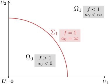
Figure 1: Sketch of the regions $\Omega_{0}$ and $\Omega_{1}$ and the first unitary limit surface $\Sigma_{1}\subset\Omega_{1}$ for the degree $d=2$ of discretization. In this specific case, the potential space $\Omega$ is the first quadrant of $\mathbb{R}^{2}$ and unitary limit surfaces are one-dimensional manifolds.

Predicting $f$ with an ensemble of MLPs: The factor $f$ seems to be a powerful quantity for describing the geometry of the unitary limit surface $\Sigma_{1}$, the latter is merely the contour for $f=1$. It is a simple task to derive $f$ iteratively by scaling a given potential $\bm{U}$ until the scattering length flips its sign SM . However, an analytic relation between $\bm{U}$ and $f$ remains unknown to us. The remedy for this are neural networks that are trained supervisedly on pairs $(\bm{U},f)\in T_{1}$ of potentials (inputs) and corresponding factors (targets) in some training set $T_{1}$. In this case, neural networks can be understood as maps $\mathcal{F}:\Omega\to\mathbb{R}$ that additionally depend on numerous internal parameters. The key idea of supervised training is to adapt the internal parameters iteratively such that the outputs $\mathcal{F}(\bm{U})$ approach the targets $f$ ever closer. As a result of training, $\mathcal{F}$ approximates the underlying function $\bm{U}\mapsto f$, such that the factor $f^{*}\approx\mathcal{F}(\bm{U}^{*})$ is predicted with sufficient accuracy even if the potential $\bm{U}^{*}\in\Omega$ does not appear in the training set, as long as it resembles the potentials encountered during training. In order to measure the performance of $\mathcal{F}$ on unknown data, one considers a test set $T_{2}$ containing previously unknown pairs $(\bm{U}^{*},f^{*})$ and the mean average percentage error (MAPE) on that data set,

$$\text{MAPE}=\frac{1}{|T_{2}|}\sum\limits_{(\bm{U}^{*},f^{*})\in T_{2}}\left|\frac{\mathcal{F}(\bm{U}^{*})-f^{*}}{f^{*}}\right|~{}.\vspace{-0.1cm}$$ (6)

We decide to work with MLPs. These are a widely distributed and very common class of neural networks and provide an excellent performance for simpler problems. Here, an MLP $\mathcal{F}_{i}$ with $L$ layers is a composition

$$\mathcal{F}_{i}=Y_{L}\circ\ldots\circ Y_{1}\vspace{-0.15cm}$$ (7)

of functions $Y_{j}:~{}V_{j-1}\to V_{j}$. Usually we have $V_{j}=\mathbb{R}^{h_{j}}$. While $Y_{1}:\Omega\to V_{1}$ and $Y_{L}:V_{L-1}\to\mathbb{R}$ are called the input and output layers, respectively, each intermediate layer is referred to as a hidden layer. The layer $Y_{j}$ depends on a weight matrix $W_{j}~{}\in~{}\mathbb{R}^{h_{j}\times h_{j-1}}$ and a bias $\bm{b}_{j}\in\mathbb{R}^{h_{j}}$, both serving as internal parameters, and performs the operation

$$Y_{j}(\bm{v})=a_{j}(W_{j}\bm{v}+\bm{b}_{j})\vspace{-0.15cm}$$ (8)

on the vector $\bm{v}\in V_{j-1}$. The function $a_{j}:\mathbb{R}\to\mathbb{R}$ is called the activation function of the $j^{\text{th}}$ layer and is applied component-wise to vectors. Using non-linear activation functions is crucial in order to make MLPs universal approximators. While output layers are classically activated via the identity, we activate all other layers via the continuously differentiable exponential linear unit (CELU) Barron:2017 ,

$$\mathrm{CELU}(v)=\mathrm{max}(0,v)+\mathrm{min}(0,\mathrm{exp}(v)-1)~{}.\vspace{-0.2cm}$$ (9)

We use CELU because it is continuously differentiable, has bounded derivatives, allows positive and negative activations and finally bypasses the vanishing-gradient-problem, which renders it very useful for deeper architectures. In order to achieve precise predictions of the factors $f$, we decide to train an ensemble of $N_{\mathcal{F}}$ $=$ $100$ MLPs $\mathcal{F}_{i}$, with each MLP consisting of nine CELU-activated $64$ $\times$ $64$ linear layers and one output layer. The output of the ensemble is simply the mean of all individual outputs,

$$\mathcal{F}(\bm{U})=\frac{1}{N_{\mathcal{F}}}\sum\limits_{i=1}^{N_{\mathcal{F}}}\mathcal{F}_{i}(\bm{U})~{}.\vspace{-0.2cm}$$ (10)

The training and test data sets contain $|T_{1}|$ $=$ $3$ $\cdot$ $10^{4}$ and $|T_{2}|$ $=$ $2.9$ $\cdot$ $10^{3}$ samples, respectively, as described in SM . All potentials are discretized with a degree of $d$ $=$ $64$. Positive and negative scattering lengths are nearly equally represented in each data set. After $20$ epochs, that is after having scanned through the training set for the $20^{\text{th}}$ time, the training procedure is terminated and the resulting MAPE of the ensemble $\mathcal{F}$ turns out as $0.028\,\%$. When plotting predictions versus targets, this implies a thin point cloud that is closely distributed around the bisector as can be seen in Fig. 2. We therefore conclude that $\mathcal{F}$ returns very precise predictions on $f$.

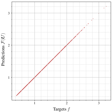
Figure 2: Predictions $\mathcal{F}(\bm{U})$ of the scaling factor by the ensemble $\mathcal{F}$ versus the targets $f$ for all $(\bm{U},f)\in T_{2}$. The resulting point cloud is very closely distributed around the bisector, which indicates an excellent performance of $\mathcal{F}$ on the test set $T_{2}$.

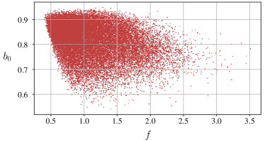
Figure 3: $b_{0}$ versus the corresponding factors $f$ for all potentials $\bm{U}$ in the training set $T_{1}$. Note that $b_{0}$ is restricted to a small interval. The width of the point cloud suggests that there is no one-to-one relation between $b_{0}$ and $f$.

Predicting scattering lengths in vicinity of $\mathit{\Sigma_{1}}$: As shown in the previous section, training an ensemble of MLPs to reproduce the factors $f$ for given potentials $\bm{U}\in\Omega$ is a numerically simple approach for investigating the unitary limit surface $\Sigma_{1}$. Our key motivation is to predict scattering lengths in the vicinity of unitary limit surfaces by using neural networks. However, the unitary limit itself poses a major obstacle to common neural networks and training algorithms: Reproducing the movable singularity for $a_{0}$ on $\Sigma_{1}$ imposes severe restrictions on the MLP architecture and renders the training steps unstable. Thus we must pursue alternative approaches. The idea of the approach we opt for is to express scattering lengths in terms of regular quantities, that each can be easily predicted by MLPs. Therefore we first consider the quantity

$$b_{0}=a_{0}(1-f)=\frac{a_{0}x}{\|\bm{U}\|}~{}.\vspace{-0.1cm}$$ (11)

As shown in Fig. 3, $b_{0}$ is finite and restricted to a small interval for all potentials in the training set. We therefore expect training MLPs to predict $b_{0}$ to be a numerically simple task. This again suggests to train an ensemble $\mathcal{B}$ of $N_{\mathcal{B}}=100$ MLPs $\mathcal{B}_{i}$,

$$\mathcal{B}(\bm{U})=\frac{1}{N_{\mathcal{B}}}\sum\limits_{i=1}^{N_{\mathcal{B}}}\mathcal{B}_{i}(\bm{U})~{}.\vspace{-0.15cm}$$ (12)

While the members $\mathcal{B}_{i}$ only consist of five CELU-activated $64$ $\times$ $64$ linear layers and one output layer, the rest coincides with the training procedure of the ensemble $\mathcal{F}$ as presented in the previous section. The resulting MAPE of the ensemble $\mathcal{B}$ turns out as $0.017\,\%$, which indicates that $\mathcal{B}$ approximates the relation $\bm{U}\mapsto b_{0}$ very well around $\Sigma_{1}$.

Due to Eq. (11), scattering lengths can be expressed in terms of $b_{0}$ and $f$. Having trained the ensembles $\mathcal{B}$ and $\mathcal{F}$ to predict these two quantities precisely, we expect the quotient

$$\mathcal{A}(\bm{U})=\frac{\mathcal{B}(\bm{U})}{1-\mathcal{F}(\bm{U})}\vspace{-0.1cm}$$ (13)

to provide a good approximation of $a_{0}$ for potentials $\bm{U}$$\in$$\,\Omega$ in vicinity of $\Sigma_{1}$. However, note that outputs $\mathcal{A}(\bm{U})$ for potentials $\bm{U}$ in the unitary limit $f\to 1$ are very sensitive to $\mathcal{F}(\bm{U})$. In this regime, even the smallest errors may cause a large deviation from the target values and thereby corrupt the accuracy of $\mathcal{A}$. Let us therefore consider the relative errors of predicted scattering lengths,

$$\varepsilon_{{}_{\mathcal{A}(\bm{U})}}=\frac{\mathcal{A}(\bm{U})-a_{0}}{a_{0}}~{},\vspace{-0.2cm}$$ (14)

for potential wells $\bm{U}=u\begin{pmatrix}1,&\ldots,&1\end{pmatrix}^{T}$ with depths $u$. In Fig. 4 we observe significantly larger relative errors in a small interval around the unitary limit at $u=\pi^{2}/4$. Nonetheless, the quotient $\mathcal{A}$ reproduces the behavior of $a_{0}$ sufficiently well.

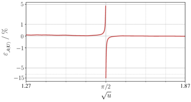
Figure 4: Relative errors $\varepsilon_{{}_{\mathcal{A}(\bm{U})}}$ of predicted scattering lengths $\mathcal{A}(\bm{U})$ for potential wells $\mathcal{U}$ with depths $u$. The $\varepsilon_{{}_{\mathcal{A}(\bm{U})}}$ only take values between $1\%$ and $15\%$ in close vicinity of the unitary limit at $u~{}=~{}\pi^{2}/4$. Otherwise, the relative errors become negligibly small.

We can also convince ourselves of this for more general potentials by inspecting the prediction-vs-target plot in Fig. 5: Although we notice a broadening of the point cloud for unnaturally large scattering lengths, the point cloud itself remains clearly distributed around the bisector. Finally, the resulting MAPE of $0.41\,\%$ indicates an overall good performance of $\mathcal{A}$ on the test set $T_{2}$.

Figure 5: Predictions $\mathcal{A}(\bm{U})$ of scattering lengths by the quotient $\mathcal{A}$ versus the targets $a_{0}$. The point cloud becomes broader for unnaturally large scattering lengths. Nonetheless it is still distributed sufficiently close around the bisector, which indicates that $\mathcal{A}$ generalizes well and reproduces the correct behavior of $a_{0}$ around $\Sigma_{1}$.

Discussion and outlook: The unitary limit $a_{0}\to\infty$ is realized by movable singularities in potential space $\Omega$, each corresponding to a hypersurface $\Sigma_{i}\subset\Omega$ that we refer to as the $i^{\text{th}}$ unitary limit surface. This formalism not only lets one understand the unitary limit in a geometric manner, but also introduces new quantities $f$ and $b_{0}$. These are regular in the unitary limit and provide an alternative parameterization of low-energy scattering processes. As such, they suffice to derive the S-wave scattering length $a_{0}$. By training ensembles of multilayer perceptrons in order to predict $f$ and $b_{0}$, respectively, we therefore successfully establish a machine learning based description for unnatural as well as natural scattering lengths.

Note that this is by far not the only reasonable approach towards the unitary limit. Another, even simpler approach would have been to train networks to predict the inverse scattering length $1/a_{0}$, which is obviously regular in the unitary limit. Considering the inverse prediction afterwards would provide a good estimate on unnatural scattering lengths, too. However, we have decided to stay in the developed formalism of unitary limit surfaces and to use the geometric quantities $f$ and $b_{0}$ to describe the unitary limit for the sake of interpretability. Concerning interpretability, it is important to note that both trained ensembles still need to be considered as “black boxes”, since we have not interpreted how inputs are processed physically, yet. An appropriate approach to mention here is the Taylor decomposition of both ensembles for expansion points on $\Sigma_{1}$ SM . This also provides additional geometric insights like normal vectors on the unitary limit surface.

Of course, this approach is also suitable for describing unitary limit surfaces of higher order. We can also think of a simultaneous treatment of several unitary limit surfaces. Also, it can be generalized to arbitrary effective range expansion parameters that produce other movable singularities in potential space. More generally, its scope is not limited to scattering problems, but can be utilized in systems that exhibit an unnaturally large scale.

We thank Bernard Metsch for useful comments. We acknowledge partial financial support from the Deutsche Forschungsgemeinschaft (TRR 110, “Symmetries and the Emergence of Structure in QCD”), Further support was provided by the Chinese Academy of Sciences (CAS) President’s International Fellowship Initiative (PIFI) (grant no. 2018DM0034) and by VolkswagenStiftung (grant no. 93562).

Supplemental Material

Preparation of data sets: In order to make potentials processable for neural networks, they have to be discretized. We associate the discretized potential $\bm{U}\in\Omega$ with the piecewise constant step potential

$$U(r)=\begin{cases}U_{1}&\text{if}\ \hskip 12.80365ptr_{0}\leq r<r_{1}~{},\\ &\vdots\\ U_{n}&\text{if}\ \hskip 12.80365ptr_{n-1}\leq r<r_{n}~{},\\ &\vdots\\ 0&\text{if}\ \hskip 12.80365ptr_{d}\leq r<r_{d+1}~{},\end{cases}$$ (15)

with the transition points $r_{n}=n/d$ for $n=0,\ldots,d$ and $r_{d+1}=\infty$. Accordingly, the $l^{\text{th}}$ partial wave is defined piecewise as well: Between the transition points $r_{n-1}$ and $r_{n}$ it is given as a linear combination of spherical Bessel and Neumann functions,

$$\phi_{n}^{(l,k)}(r)=A_{l,n}(k)j_{l}(k_{n}r)-B_{l,n}(k)n_{l}(k_{n}r)~{},$$ (16)

with the kinetic energy

$$k_{n}=\Theta_{\mathrm{Re}}(k)\sqrt{k^{2}+U_{n}\vphantom{\frac{a}{a}}}~{}.$$ (17)

Here we introduce the factor

$$\Theta_{\mathrm{Re}}(k)=\begin{cases}+1~{},&\text{if}\ \mathrm{Re}(k)\geq 0\\ -1~{},&\text{if}\ \mathrm{Re}(k)<0\end{cases}$$ (18)

to conserve the sign of $k$ on the complex plane, that is $k_{n}$ $\to$ $k$, if $U_{n}$ vanishes. The parameters $A_{l,d+1}(k)$ and $B_{l,d+1}(k)$ completely determine the effective range function $K_{l}(k)~{}=~{}k^{2l+1}~{}\cot\delta_{l}(k)$ due to their asymptotic behavior

$$A_{l,d+1}(k) =\mathrm{e}^{i\delta_{l}(k)}\cos\delta_{l}(k),$$ (19)

$$B_{l,d+1}(k) =\mathrm{e}^{i\delta_{l}(k)}\sin\delta_{l}(k)~{}.$$ (20)

Instead of solving the Schrödinger equation for the step potential $U(r)$, we apply the transfer matrix method Jonsson:1990 to derive $A_{l,d+1}(k)$ and $B_{l,d+1}(k)$. Due to the smoothness of the partial wave $\phi^{(l,k)}$ at each transition point $r_{n}$, this method allows us to relate $A_{l,d+1}(k)$ and $B_{l,d+1}(k)$ to the initial parameters $A_{l,1}(k)$ and $B_{l,1}(k)$ via a product of transfer matrices $M_{l,n}(k)$. To arrive at a representation of these transfer matrices, we split up the mentioned smoothness condition into two separate conditions for continuity,

$$\phi_{n+1}^{(l,k)}(r_{n})=\phi_{n}^{(l,k)}(r_{n})$$ (21)

and differentiability,

$$\frac{\mathrm{d}}{\mathrm{d}r}\phi_{n+1}^{(l,k)}(r)\bigg{|}_{r=r_{n}}=\frac{\mathrm{d}}{\mathrm{d}r}\phi_{n}^{(l,k)}(r)\bigg{|}_{r=r_{n}}$$ (22)

at each transition point $r_{n}$. Using Eq. (16), we can combine both conditions (21) and (22) to a vector equation, that connects neighboring coefficients with each other:

$$\underbrace{\begin{pmatrix}j_{l}(k_{n+1}r_{n})&-n_{l}(k_{n+1}r_{n})\\ k_{n+1}j_{l}^{\prime}(k_{n+1}r_{n})&-k_{n+1}n_{l}^{\prime}(k_{n+1}r_{n})\end{pmatrix}}_{=m_{l,n+1}(r_{n},k)}\begin{pmatrix}A_{l,n+1}(k)\\ B_{l,n+1}(k)\end{pmatrix}$$

$$=\underbrace{\begin{pmatrix}j_{l}(k_{n}r_{n})&-n_{l}(k_{n}r_{n})\\ k_{n}j_{l}^{\prime}(k_{n}r_{n})&-k_{n}n_{l}^{\prime}(k_{n}r_{n})\end{pmatrix}}_{=m_{l,n}(r_{n},k)}\begin{pmatrix}A_{l,n}(k)\\ B_{l,n}(k)\end{pmatrix}~{}.$$ (23)

Multiplying Eq. (23) with $m_{l,n+1}^{-1}(r_{n},k)$ from the left yields

$$\begin{pmatrix}A_{l,n+1}(k)\\ B_{l,n+1}(k)\end{pmatrix}=M_{l,n}(k)\begin{pmatrix}A_{l,n}(k)\\ B_{l,n}(k)\end{pmatrix},$$ (24)

which defines the $n^{\text{th}}$ transfer matrix

$$M_{l,n}(k)=m_{l,n+1}^{-1}(r_{n},k)m_{l,n}(r_{n},k)~{}.$$ (25)

Therefore, $A_{l,d+1}(k)$ and $B_{l,d+1}(k)$ are determined by the choice of $A_{l,1}(k)$ and $B_{l,1}(k)$, which requires us to define two boundary conditions. Due to the singularity of $n_{l}$ in the origin, the spherical Neumann contribution in the first layer must vanish and therefore $B_{l,1}(k)=0$. The choice of $A_{l,1}(k)$ may alter the normalization of the wave function. However, since we only consider ratios of $A_{l,d+1}(k)$ and $B_{l,d+1}(k)$, we may opt for $A_{l,1}(k)=1$, which corresponds to

$$\phi_{1}^{(l,k)}(r)=j_{l}(k_{1}r)~{}.$$ (26)

Finally, applying all transfer matrices successively to the initial parameters yields

$$\begin{pmatrix}A_{l,d+1}(k)\\ B_{l,d+1}(k)\end{pmatrix}=\left(\prod\limits_{n=1}^{d}M_{l,n}(k)\right)\ \begin{pmatrix}1\\ 0\end{pmatrix}~{}.$$ (27)

The most general way to derive any effective range expansion parameter $Q_{l}^{(j)}(\varkappa)$ for arbitrary expansion points $\varkappa\in\mathbb{C}$ in the complex momentum plane is a contour integration along a circular contour $\gamma$ with radius $\kappa_{\gamma}$ around $\varkappa$. Applying Cauchy’s integral theorem then yields

$$Q_{l}^{(j)}(\varkappa) =\frac{1}{2\pi i}\oint_{\gamma}\!\mathrm{d}k\,\frac{k^{2l+1}}{(k-\varkappa)^{j+1}}\frac{A_{l,d+1}(k)}{B_{l,d+1}(k)}~{}.$$ (28)

We approximate this integral numerically over $N$ grid points

$$k_{q}=\varkappa+\kappa_{\gamma}\mathrm{e}^{iq{2\pi}/{N}},\hskip 28.45274ptq=0,\ldots,N-1~{}.$$ (29)

Smaller contour radii $\kappa_{\gamma}$ and larger $N$ thereby produce finer grids and decrease the approximation error. This way of calculating $Q_{l}^{(j)}(\varkappa)$ requires in total $d$ $\times$ $N$ transfer matrices. The numerical integration provides

$$Q_{l}^{(j)}(\varkappa)\approx\frac{1}{N(\kappa_{\gamma})^{j}}\sum\limits_{q=0}^{N-1}(k_{q})^{2l+1}\mathrm{e}^{-iq\frac{2\pi}{N}}\frac{A_{l,d+1}(k_{q})}{B_{l,d+1}(k_{q})}~{}.$$ (30)

Despite the generality of Eq. (30), we restrict this analysis to $S$-wave scattering lengths $a_{0}$ $=$ $-1/Q_{0}^{(0)}(0)$, since these dominate low-energy scattering processes.

While generating the training and test sets, we must ensure that there are no overrepresented potential shapes among the respective data set. To maintain complexity, this suggests generating potentials with randomized components $U_{n}$. An intuitive approach therefore is to produce them via Gaussian random walks: Given $d$ normally distributed random variables $X_{1},\ldots,X_{d}$,

$$X_{i}\sim\begin{cases}\mathcal{N}(0,\mathrm{ISF})&\text{if}\ i=1~{},\\ \mathcal{N}(0,\mathrm{SF})&\text{else}~{},\end{cases}$$ (31)

where $\mathcal{N}(\mu,\sigma)$ describes a normal distribution with mean $\mu$ and standard deviation $\sigma$, the distribution of the $n^{\text{th}}$ potential step $U_{n}$ can be described by the magnitude of the sum over all previous steps $X_{i}$,

$$U_{n}=\left|\sum\limits_{i=1}^{n}X_{i}\right|~{}.$$ (32)

Note that, while all steps $X_{i}$ in Eq. (31) have zero mean, the standard deviation of the first step, which we denote by the initial step factor $\mathrm{ISF}$, may differ from the standard deviation of all other steps, that we refer to as the step factor $\mathrm{SF}$. This allows us to roughly control the shapes and depths of all potentials in the data set. Choosing $\mathrm{ISF}\gg\mathrm{SF}$ results more likely in potentials that resemble a potential well and expectedly yield similar scattering lengths. In contrast to that, $\mathrm{SF}\gg\mathrm{ISF}$ produces strongly oscillating potentials. We decide to choose the middle course $\mathrm{ISF}=1$ and $\mathrm{SF}=0.75$ (this is the case $\mathrm{SF}\approx\mathrm{ISF}$) for two reasons: For one, from the perspective of depths, the corresponding Gaussian random walk is capable of generating potentials around the first unitary limit surface $\Sigma_{1}$. For another, this choice of step factors causes the data set to cover a wide range of shapes from dominantly potential wells to more oscillatory potentials, which is an important requirement for generalization. This way, we generate $10^{5}$ potentials for the training set and $10^{4}$ potentials for the test set, To avoid overfitting to a certain potential depth, this needs to be followed by a rigorous downsampling procedure. For this, we use the average depth

$$u=\frac{1}{d}\sum\limits_{n=1}^{d}U_{n}$$ (33)

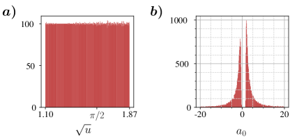
Figure 6: $a):$ Distribution of the square root $\sqrt{u}$ of the average depth over the training set. By construction, this distribution is uniform. $b):$ Bimodal distribution of the scattering length $a_{0}$ over the training set. Note that extremely large scattering lengths are not displayed in this histogram.

as a measure. Uniformizing the training and test set with respect to $\sqrt{u}$ on the interval $[1.10,1.87]$ by randomly omitting potentials with overrepresented depths finally yields a training set $T_{1}$, see Fig. 6, and test set $T_{2}$ that contain $3\times 10^{4}$ and $2.9\times 10^{3}$ potentials, respectively. Scattering lengths are then derived using the numerical contour integration in Eq. (30) with $N=100$ grid points and a contour radius of $\kappa_{\gamma}=0.1$. The derivation of the factors $f$ is more involved: If the scattering length is negative (positive), the potential is iteratively scaled with the factor $s=2$ ($s=1/2$), until its scattering length changes its sign. Let us assume the potential has been scaled $t$ times this way. Then we can specify the interval where we expect to find $f$ in as $(2^{t-1},2^{t}]$ or as $[2^{-t},2^{1-t})$, respectively. Cubically interpolating $1/a_{0}$ on that interval using $25$ equidistant values and searching for its zero finally yields the desired factor $f$.

Training by gradient descent: Given a data set $D$ $\subseteq$ $\Omega$ $\times$ $\mathbb{R}^{n}$, there are several ways to measure the performance of a neural network $\mathcal{N}:\Omega\to\mathbb{R}^{n}$ on $D$. For this we have already introduced the MAPE that we have derived for the test set $D=T_{2}$ after training. Lower MAPEs are thereby associated with better performances. Such a function $L:\Gamma\to\mathbb{R}^{+}$ that maps a neural network to a non-negative, real number is called a loss function. The weight space $\Gamma$ is the configuration space of the used neural network architecture and as such it is spanned by all internal parameters (e.g. all weights and biases of an MLP). Therefore, we can understand all neural networks $\mathcal{N}\in\Gamma$ of the given architecture as points in weight space. The goal all training algorithms have in common is to find the global minimum of a given loss function in weight space. It is important to note that loss functions become highly non-convex for larger data sets and deeper and more sophisticated architectures. As a consequence, training usually reduces to finding a well performing local minimum.

A prominent family of training algorithms are gradient descent techniques. These are iterative with each iteration corresponding to a step the network takes in weight space. The direction of the steepest loss descent at the current position $\mathcal{N}\in\Gamma$ is given by the negative gradient of $L(\bm{t},\mathcal{N}(\bm{U}))$. Updating internal parameters along this direction is the name-giving feature of gradient descent techniques. This suggests the update rule

$$p\longleftarrow p-\eta\frac{\partial L}{\partial p}(\bm{t},\mathcal{N}(\bm{U}))$$ (34)

for each internal parameter $p$, and by the left arrow $a~{}\longleftarrow~{}b$ we denote the assignment ’a=b’ as used in computer programming. Accordingly, the entire training procedure corresponds to a path in weight space. The granularity of that path is controlled by the learning rate $\eta$: Smaller learning rates cause a smoother path but a slower approach towards local minima and vice versa. In any case, training only for one epoch, that is scanning only once through the training set, usually does not suffice to arrive near any satisfactory minima. A typical training procedure consists of several epochs.

Usually, the order of training samples $(\bm{U},\bm{t})$ is randomized to achieve a faster learning progress and to make training more robust to badly performing local minima. Therefore, this technique is also called stochastic gradient descent. Important alternatives to mention are mini-batch gradient descent and batch gradient descent, where update steps are not taken with respect to the loss $L(\bm{t},\mathcal{N}(\bm{U}))$ of a single sample, but to the batch loss

$$L_{D}(\mathcal{N})=\frac{1}{|D|}\sum\limits_{(\bm{U},\bm{t})\in D}L(\bm{t},\mathcal{N}(\bm{U}))$$ (35)

of randomly selected subsets $D$ of the training set $T_{1}$ with the batch size $|D|=B$ or the entire training set itself, respectively. There are more advanced gradient descent techniques like Adam and Adamax Kingma:2017 that introduce a dependence on previous updates and adapted learning rates. It is particularly recommended to use these techniques when dealing with large amounts of data and high-dimensional weight spaces.

For training the members $\mathcal{F}_{i}$ and $\mathcal{B}_{i}$ of both ensembles $\mathcal{F}$ and $\mathcal{B}$, we apply the same training procedure using the machine learning framework provided by PyTorch Paszke:2019 : Weights and biases are initialized via the He-initialization He:2015 . We use the Adamax optimizer with the batch size $B=10$ to minimize the L1-Loss,

$$L_{\text{L1}}(\bm{t},\mathcal{N}(\bm{U}))=\frac{1}{n}\|\bm{t}-\mathcal{N}(\bm{U})\|,$$ (36)

over $20$ epochs. Here, we apply an exponentially decaying learning rate schedule, that is $\eta_{t}=0.01\ \exp(-t/2)$ is epoch dependent. In this case, the decreasing learning rates allow a much closer and more stable approach towards local minima.

Neural network ensembles: Each ensemble $\mathcal{F}$ and $\mathcal{B}$ consists of $100$ MLPs. In the above framework, an ensemble can be understood as a point cloud in weight space. We can assume that each of these members is close to a well performing local minimum or even to the global minimum. There are several techniques to let the ensemble vote on one, even more precise prediction. Here, we choose to take the average of all individual predictions. We observe a significant increase in accuracy (by almost a factor of two) by comparing the resulting MAPEs of $\mathcal{F}$ and $\mathcal{B}$ with the individual MAPEs of the members, shown in Figs. 7a) and 7b).

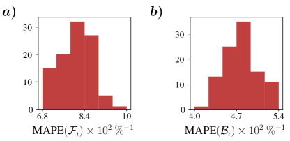
Figure 7: $a):$ Individual MAPEs of the members $\mathcal{F}_{i}$ of the ensemble $\mathcal{F}$. $b):$ Individual MAPEs of the members $\mathcal{B}_{i}$ of the ensemble $\mathcal{B}$.

Figure 8: Predictions of natural and unnatural scattering lengths for potential wells $\bm{U}=u\begin{pmatrix}1,\ldots,1\end{pmatrix}$ by the quotient $\mathcal{A}$. Note that the shown graph reproduces the expected behavior $a_{0}$ $=$ $1$ $-$ $\tan\sqrt{u}/\sqrt{u}$ very well.

Taylor expansion to restore interpretability: Considering the quotient $\mathcal{A}(\bm{U})$$=$$\mathcal{B}(\bm{U})$$/$$(1$$-$$\mathcal{F}(\bm{U}))$, we can make reliable predictions on natural and unnatural scattering lengths, c.f. Fig. 8. We have established a geometrical understanding of the quantities $f$ and $b_{0}$, predicted by $\mathcal{F}$ and $\mathcal{B}$, respectively. However, since both ensembles are “black boxes”, their outputs and the outputs of $\mathcal{A}$ are no longer interpretable beyond that level. One way to restore interpretability is to consider the Taylor expansion with respect to an appropriate expansion point. In the following, we demonstrate this for the ensemble $\mathcal{F}$ on the first unitary limit surface: Since $\mathcal{F}$ is regular in the expansion point $\bm{U}^{*}\in\Sigma_{1}$, its Taylor series can be written as

$$\mathcal{F}(\bm{U})=\mathcal{F}(\bm{U}^{*})+\bm{n\cdot\delta U}+\mathcal{O}(\bm{\delta U}^{2})$$ (37)

with the displacement $\bm{\delta U}=\bm{U}-\bm{U}^{*}$ and the vector $\bm{n}$ with the components

$$n_{i}=\frac{\partial\mathcal{F}}{\partial Y_{a}}\bigg{|}_{\bm{Y}=\bm{U}^{*}}~{}.$$ (38)

For small displacements $\|\bm{\delta U}\|\ll 1$ higher order terms in Eq. (37) can be ignored. From construction we know that $\mathcal{F}(\bm{U}^{*})\approx 1$ for any $\bm{U}^{*}\in\Sigma_{1}$, since $f=1$. Note that the vector $\bm{n}$ is the normal vector of the first unitary limit surface at the point $\bm{U}^{*}$. This is because $\mathcal{F}(\bm{U})$ is invariant under infinitesimal, orthogonal displacements $\bm{\delta U}\bot\ \bm{n}$, i.e. tangential displacements to $\Sigma_{1}$.

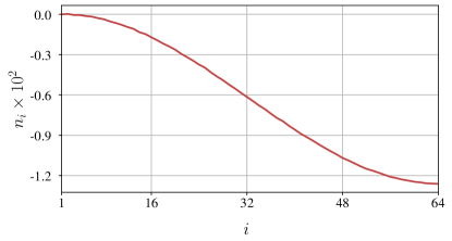
Figure 9: Components of the normal vector $\bm{n}$ of the unitary limit surface at $\bm{U}^{*}=\pi^{2}/4\begin{pmatrix}1,\ldots,1\end{pmatrix}$. As a gradient of $\mathcal{F}$, this vector points towards the strongest ascent of $f$, which explains why its components are not positive.

To give an example, we consider the first order Taylor approximation for the expansion point $\bm{U}^{*}=\pi^{2}/4\begin{pmatrix}1,\ldots,1\end{pmatrix}$. This corresponds to an expansion around the potential well with exactly one bound state that is also a zero-energy bound state. At first we derive $\mathcal{F}(\bm{U}^{*})=1-3.2\times 10^{-5}\approx 1$. Due to the rather involved architecture of $\mathcal{F}$, we decide to calculate derivatives numerically,

$$\vspace{-2mm}n_{i}\approx\frac{\mathcal{F}(\bm{U}^{*}+\Delta\bm{e}_{i})-\mathcal{F}(\bm{U}^{*})}{\Delta}\vspace{-1mm}$$ (39)

with the $i^{\text{th}}$ basis vector $\bm{e}_{i}$ and the step size $\Delta=0.01$. The resulting components of the normal vector are depicted in Fig. 9. In this case, we can clearly see that $\bm{n}$ is far from collinear to $\bm{U}^{*}$, which indicates that $\Sigma_{1}$ may have a rather complicated topology. Using the expansion in Eq. (37) and the components $n_{i}$ shown in Fig. 4, we arrive at an interesting and interpretable approximation of $\mathcal{A}(\bm{U})$ around $\bm{U}^{*}$,

$$\mathcal{A}(\bm{U})\approx-\frac{\mathcal{B}(\bm{U}^{*})}{\bm{n\cdot\delta U}}~{},$$ (40)

which lets us model the unitary limit in terms of a scalar product. Let us consider displacements $\bm{\delta U}=$ $(u$$-$$\pi^{2}/4)$$\begin{pmatrix}1,\ldots,1\end{pmatrix}$ that are parallel to $\bm{U}^{*}$. Inserting the value $\mathcal{B}(\bm{U}^{*})=0.81$ and $\sum_{i}n_{i}=-0.40$, Eq. (40) becomes

$$\mathcal{A}(\bm{U})\approx\frac{2.01}{u-{\pi^{2}}/{4}}~{}.$$ (41)

We can compare this to the expected behavior $a_{0}$$=$$1$$-$$\tan\sqrt{u}/\sqrt{u}$ of the S-wave scattering length for potential wells. The Padé-approximant of order $[0/1]$ of this function at the point $u=\pi^{2}/4$ is given by

$$a_{0}\approx\frac{2}{u-{\pi^{2}}/{4}}~{},$$ (42)

which agrees very well with the approximation Eq. (41) of scattering length predictions for inputs $\bm{U}=~{}u\begin{pmatrix}1,\ldots,1\end{pmatrix}$ in the vicinity of $\bm{U}^{*}$ by the quotient $\mathcal{A}$.

References

- (1) A. Radovic, M. Williams, D. Rousseau et al. Nature 560, 41 (2018).
- (2) J. W. Richards et al., Astrophys. J. 733, 10 (2011).
- (3) A. Buckley, A. Shilton and M. J. White, Comput. Phys. Commun. 183, 960 (2012).
- (4) P. Graff, F. Feroz, M. P. Hobson and A. N. Lasenby, Mon. Not. Roy. Astron. Soc. 441, 1741 (2014).
- (5) G. Carleo and M. Troyer, Science 355, 602 (2017).
- (6) K. Mills, M. Spanner and I. Tamblyn, Phys. Rev. A 96, 042113 (2017).
- (7) S. J. Wetzel and M. Scherzer, Phys. Rev. B 96, 184410 (2017).
- (8) Y. H. He, Phys. Lett. B 774, 564 (2017).
- (9) Y. Fujimoto, K. Fukushima and K. Murase, Phys. Rev. D 98, 023019 (2018).
- (10) Y. Wu, P. Zhang, H. Shen and H. Zhai, Phys. Rev. A 98, 010701 (2018).
- (11) Z. M. Niu, H. Z. Liang, B. H. Sun, W. H. Long and Y. F. Niu, Phys. Rev. C 99, 064307 (2019).
- (12) J. Brehmer, K. Cranmer, G. Louppe and J. Pavez, Phys. Rev. Lett. 121, 111801 (2018).
- (13) J. Steinheimer, L. Pang, K. Zhou, V. Koch, J. Randrup and H. Stoecker, JHEP 1912, 122 (2019).
- (14) A. J. Larkoski, I. Moult and B. Nachman, Phys. Rept. 841, 1 (2020).
- (15) V. Efimov, Phys. Lett. 33B, 563 (1970).
- (16) H. Heiselberg, Phys. Rev. A 63, 043606 (2002).
- (17) E. Braaten and H.-W. Hammer, Phys. Rept. 428, 259 (2006).
- (18) A. Bulgac, J. E. Drut and P. Magierski, Phys. Rev. Lett. 96, 090404 (2006).
- (19) D. Lee, Phys. Rev. B 73, 115112 (2006).
- (20) S. König, H. W. Grießhammer, H. W. Hammer and U. van Kolck, Phys. Rev. Lett. 118, 202501 (2017).
- (21) T. Kraemer, M. Mark, P. Waldburger, J. G. Danzl, C. Chin, B. Engeser, A. D. Lange, K. Pilch, A. Jaakkola, H.-C. Nägerl and R. Grimm, Nature 440, 315 (2006).
- (22) see the attached Supplemental Material.
- (23) J.T. Barron, arXiv:1704.07483 [cs.LG] (2017).

References

- (1) B. Jonsson, S.T. Eng, IEEE journal of quantum electronics 26.11 (1990), pp. 2025-2035.
- (2) D.P. Kingma, J. Ba, arXiv:1412.6980 [cs.LG].
- (3) K. He, X. Zhang, S. Ren and J. Sun, 2015 IEEE International Conference on Computer Vision (ICCV), pp. 1026-1034 (2015).
- (4) A. Paszke, S. Gross, F. Massa, A. Lerer, J. Bradbury, G. Chanan, T. Killeen, Z. Lin, N. Gimelstein, L. Antiga, A. Desmaison, A. Kopf, E. Yang, Z. DeVito, M. Raison, T. Alykhan, S. Chilamkurthy, B. Steiner, F. Lu, J. Bai and S. Chintala, in: Advances in Neural Information Processing Systems 32 (2019), pp. 8024-8035 (eds. H. Wallach, H. Larochelle, A. Beygelzimer, F. d’Alché-Buc, E. Fox and R. Garnett).