Modelling of the Effects of Stellar Feedback during Star Cluster Formation Using a Hybrid Gas and N-Body Method

Abstract

Understanding the formation of stellar clusters requires following the interplay between gas and newly formed stars accurately. We therefore couple the magnetohydrodynamics code FLASH to the N-body code ph4 and the stellar evolution code SeBa using the Astrophysical Multipurpose Software Environment (AMUSE) to model stellar dynamics, evolution, and collisional N-body dynamics and the formation of binary and higher-order multiple systems, while implementing stellar feedback in the form of radiation, stellar winds and supernovae in FLASH. We use this novel numerical method to simulate the formation and early evolution of open clusters of $\sim 1000$ stars formed from clouds with a mass range of ${10}^{3}\text{\,}\textrm{M}_{\odot}{10}^{5}\text{\,}\textrm{M}_{\odot}$. Analyzing the effects of stellar feedback on the gas and stars of the natal cluster, we find that in these examples, the stellar clusters are resilient to disruption, even in the presence of intense feedback. This can even slightly increase the amount of dense, Jeans unstable gas by sweeping up shells; thus, a stellar wind strong enough to trap its own H ii region shows modest triggering of star formation. Our clusters are born moderately mass segregated, an effect enhanced by feedback, and retained after the ejection of their natal gas, in agreement with observations.

tablenum SIXtablenum

1 Introduction

Star cluster formation is a nonlinear, attenuated, feedback problem: initially cold and dense gas starts forming stars, and the more dense gas is available, the more vigorous the star formation becomes (Mac Low & Klessen, 2004). However as the number of stars increase, so do the chances of producing multiple OB stars that can prevent further star formation by injection of kinetic energy, momentum, and radiation in surrounding regions extending out to parsecs. This feedback can not only make the gas Jeans stable, thereby halting star formation, but can also eject the gas from the natal cluster altogether. If the gas dominates the gravitational potential of the cluster at the time of ejection, the cluster may be disrupted by the gas expulsion entirely (Baumgardt & Kroupa, 2007), perhaps providing an explanation for the 90% destruction rate of all young clusters found by Lada & Lada (2003).

Stellar feedback in the context of entire clusters has been studied by several authors. Early work included radiation (Peters et al., 2010b; Krumholz et al., 2011) and winds (Krumholz et al., 2012), as well as studying the effects of clustered supernovae (Joung & Mac Low, 2006). In a seminal series of papers Dale and coauthors used a smooth particle hydrodynamics code (Monaghan, 1992) to study radiation (Dale et al., 2012a, 2013a) and winds (Dale et al., 2013b) independently as well as in combination (Dale et al., 2014, 2015a) for their effects on natal gas clouds. Subsequent studies have further investigated feedback in the form of radiation (Rosen et al., 2016; Peters et al., 2017; Vázquez-Semadeni et al., 2017; Kim et al., 2018), winds (Gatto et al., 2017), and supernovae (Kim & Ostriker, 2015; Simpson et al., 2015; Ibáñez-Mejía et al., 2016; Girichidis et al., 2016) with increasing accuracy. However none of these works has included at the same time ionizing radiation, winds, supernovae, stellar evolution, and collisional N-body dynamics capable of following the formation and dynamical evolution of wide binaries and multiple systems.

Our goal is to predict the initial conditions of a newly born star cluster: A cluster formed star by star from magnetized gas and remaining gravitationally bound during the gas expulsion process driven by stellar feedback from evolving massive stars. The gravitationally bound state of young star clusters has been supported by both observations (Tobin et al., 2009; Karnath et al., 2019) and previous simulations of young clusters (Offner et al., 2009), although more recent studies have suggested many young stellar groups may actually be supervirial or unbound (Gouliermis, 2018; Kuhn et al., 2019). We are cautious with regard to observational claims of supervirial ratios, though, as mass segregation has been shown to bias virial measures towards smaller group masses and more unbound configurations (Fleck et al., 2006).

Our simulations bridge the gap between gas-dominated, star-formation simulations and gas-free, N-body, star cluster simulations. In a previous paper (Wall et al., 2019, hereafter Paper I), we explained how we use the AMUSE framework (Pelupessy et al., 2013; Portegies Zwart et al., 2013; Portegies Zwart & McMillan, 2019) to couple the adaptive mesh refinement magnetohydrodynamics (MHD) code FLASH (Fryxell et al., 2000), the N-body code ph4 (McMillan et al., 2012), the stellar evolution code SeBa (Portegies Zwart & Verbunt, 1996), and a treatment of tight multiple systems (using multiples Portegies Zwart & McMillan, 2019). In the current study we focus on describing the numerical methods developed to implement stellar feedback of the stars acting on gas, and their consequences. The structure of this study is as follows: In Sect. 2 we describe our particular implementations of radiation, stellar winds and supernovae. Further we discuss our modifications to FLASH for far ultraviolet and cosmic-ray background heating as well as our atomic, molecular and dust cooling approach. In Sect. 3 we describe four simulations conducted with our code; while in Sect. 4 to examine the effects of feedback on star formation, cluster structure, and the possibility of triggering star formation through stellar feedback. Finally we close in Sect. 5 with a summary.

The source code for our method, including our new and revised routines for FLASH and the bridge script to couple FLASH and AMUSE, are available at https://bitbucket.org/torch-sf/torch/. Documentation available is summarized at https://torch-sf.bitbucket.io/. We invite community use of this method and participation in its further development.

2 Feedback Implementation

In Paper I we described our star formation method. In short, sink particles (Bate et al., 1995; Krumholz et al., 2004; Federrath et al., 2010) form in regions of dense, gravitationally bound gas. As soon as a sink forms, a list of stars is drawn by Poisson sampling from a Kroupa (2001) initial mass function (IMF) with a minimum and maximum mass, using the same method as Sormani et al. (2017). As the sink accumulates enough mass to form the next star on the list, that star is immediately formed with position and velocity chosen based on distributions around the sink values. In the initial models described here we used Gaussians with width given by the local sound speed and the sink radius. The sink then moves to the nearest local density maximum and continues accreting.

The minimum mass is chosen in the models presented to be the hydrogen-burning limit of 0.08$\textrm{M}_{\odot}$. The maximum mass of a star is correlated with the mass of the final cluster, a result found in observations and parameterized by Weidner et al. (2010). We preserve this correlation by choosing the maximum mass that a star can obtain using their integrated galactic IMF. We calculate the maximum mass of a star assuming a given star formation efficiency $\epsilon_{\rm sfe}$ for conversion of gas into stars, taken to be unity in our present work, from our initial clouds of mass ${10}^{3}\text{\,}\textrm{M}_{\odot}{10}^{5}\text{\,}\textrm{M}_{\odot}$. This gives us a maximum mass for our ${10}^{3}\text{\,}\textrm{M}_{\odot}$ runs of $\sim$30\text{\,}\textrm{M}_{\odot}$$ and a maximum mass for the ${10}^{5}\text{\,}\textrm{M}_{\odot}$ runs of $\sim$110\text{\,}\textrm{M}_{\odot}$$.

2.1 Radiation

2.1.1 Photoionization

For radiation transport we use the FLASH module FERVENT (Baczynski et al., 2015). This module follows the ray tracing algorithm implemented in ENZO by Wise & Abel (2011). The method creates rays from point sources along directions defined using the HEALPIX (Górski et al., 2005) tiling of a sphere, then traces these rays through the block-structured, adaptively refined grid. The number of rays from a specific source hitting each individual block (usually $8^{3}$ or $16^{3}$ cells) is kept constant by splitting rays when necessary. As each ray intersects a cell the number of photons is reduced by absorption while the gas in the cell is ionized and heated accordingly.

The FERVENT package calculates the ionization fraction due to ultraviolet (UV) radiation (Baczynski et al., 2015)

$$\frac{dx_{\rm H^{+}}}{dt}=C_{\rm cl}n_{\rm e}x_{\rm H^{0}}+k_{\rm ion}x_{\rm H^{0}}-\alpha_{\rm B}n_{\rm e}x_{\rm H^{+}}.$$ (1)

Here $x_{n}$ is the fraction of species $n$, $C_{\rm cl}(T)$ is the collisional ionization rate, $\alpha_{\rm B}(T)$ is the case B recombination coefficient, $n_{\rm H}$ is the number density of neutral hydrogen, $n_{\rm e}$ is the number density of electrons and

$$k_{\rm ion}=\frac{N_{\gamma}}{n_{\rm H}(1-x)V\delta t}$$ (2)

is the rate of photon ionization, specifically formulated to be photon conservative (Baczynski et al., 2015). Here $N_{\gamma}$ is the number of photons, $V$ is the volume of a cell, $x_{\rm H^{+}}$ is the hydrogen ionization fraction, shortened hereafter to $x$, and $\delta t$ is an ionization time step.

Equation (1) was originally solved explicitly. Since we only follow hydrogen ionization, we have modified this method of FERVENT to implicitly solve the ionization evolution, which allows for a solution with a much longer time step. First we rewrite Equation 1 with substitutions for the fractional ionization $x$ everywhere

$$f(x)=\frac{dx}{dt} = C_{\rm cl}xn_{\rm H}-C_{\rm cl}x^{2}n_{\rm H}+$$

$$+k_{\rm ion}-k_{\rm ion}x-\alpha_{\rm B}x^{2}n_{\rm H},$$

then approximate it with a forward finite difference equation

$$\frac{x_{1}-x_{0}}{\delta t}={}k_{\rm ion}(C_{\rm cl}n_{\rm H}-k_{\rm ion})x_{1}-(C_{\rm cl}+\alpha_{\rm B})n_{\rm H}x^{2}_{1},$$ (4)

which is quadratic in the ionization $x_{1}$ at time $t+\delta t$, leading to an algebraic solution for $x_{1}$.

The error in this method is given by the next term in the Taylor expansion of the method,

$$x_{1}-x_{0}=f(x_{1})\delta t+\frac{f^{\prime}(x_{1})}{2}\delta t^{2},$$ (5)

which can be used to derive a more accurate estimate of the time step than the original method:

$$\delta t_{\rm ion}=\frac{c}{C_{\rm cl}n_{\rm H}-2n_{\rm H}x_{1}\left(C_{\rm cl}+\alpha_{\rm B}\right)},$$ (6)

where $c$ is a tunable safety parameter that we usually set to 0.8. (Our solutions do not seem sensitive to the exact value of $c$.) Since ionization depends strongly on the radiation field and the temperature, and rapidly converges once these fields find steady states, integration of the ionization differential equation can capture the proper timescale for each of these events. Basing the time step on the rate of change of ionization allows us to do this, while the implicit solution guarantees stability.

We have implemented subcycling on the ray tracing, ionization and heating/cooling within a single MHD time step to allow the gas dynamical time steps to be as large as possible. This results in an overall speedup of FLASH of about an order of magnitude compared to calling the (expensive) gravity and MHD solvers during the short ionization time steps.

2.1.2 Radiation Sources

To calculate stellar radiation fluxes (and winds) based on mass we only consider stars with $M>$$7\text{\,}\textrm{M}_{\odot}$. These stars are evolved using the stellar evolution code SeBa (Portegies Zwart & Verbunt, 1996, with updates from Toonen et al. 2016, who included triple evolution), which is integrated into the AMUSE framework. The luminosity $N_{\gamma}$ and average energy $\nu_{\gamma}$ of ionizing photons from these stars is calculated from their mass and age-dependent surface temperature interpolation of the OSTAR2002 grid from (Lanz & Hubeny, 2003) if the star has a surface temperature $T_{*}>$$27.5\text{\times}{10}^{3}\text{\,}\mathrm{K}$; or else just an estimate from integrating the blackbody emission $B(\lambda)$ as a function of wavelength $\lambda$ for the star if $T_{*}<$$27.5\text{\times}{10}^{3}\text{\,}\mathrm{K}$ (e.g. Stahler & Palla, 2004). Then the cross section $\sigma$ for the photons is calculated from $\nu_{\gamma}$ (Osterbrock & Ferland, 2006)

$$\sigma_{\rm H}=\sigma_{0}\left(\frac{\nu_{\gamma}}{\nu_{\rm$13.6\text{\,}\mathrm{e}\mathrm{V}$}}\right)^{-3},$$ (7)

with $\sigma_{0}=$6.304\text{\times}{10}^{-18}\text{\,}\mathrm{c}\mathrm{m}^{2}$$ (Draine, 2011a).

2.1.3 Photoelectric Effect from Far Ultraviolet

As a second energy bin for radiation we also include far ultraviolet (FUV) radiation ($5.6\text{\,}\mathrm{e}\mathrm{V}13.6\text{\,}\mathrm{e}\mathrm{V}$) which is absorbed by dust, ejecting photoelectrons in the process. Especially for lower mass stars ($7\leq M/\textrm{M}_{\odot}\leq 13$), the power in this radiation bin approaches that of photoionizing radiation. Since the cross section of photoelectric photons is smaller than those that ionize hydrogen, these rays penetrate farther into the gas, heating it farther from the source star than the ionizing radiation.

Although only about one in ten FUV photons ejects an electron from the dust, all impart momentum to the gas that can be important in clearing dense gas around newly formed massive stars. Indeed, at our typical numerical resolution, this radiation pressure is the main process acting to clear gas out of zones with densities $n_{\rm H}\gtrsim${10}^{6}\text{\,}\mathrm{c}\mathrm{m}^{-3}$$ surrounding early B and late O type stars with weak stellar winds. If this process is not implemented, the ionizing radiation from the star is trapped in the zone, producing an unphysical ultracompact H ii region.

We limit dust to gas with temperatures less than $T_{\rm sputter}=$3\text{\times}{10}^{6}\text{\,}\mathrm{K}$$ to ensure that gas does not cool unphysically in regions where dust would have previously been destroyed. This is an estimate based on the temperatures at which dust would sputter within the period that we model (Draine, 2011a, eqs. 25.13 and 25.14).

To compute the attenuation of radiation in the FUV with luminosity $N_{\gamma}$, we follow the method of the original FERVENT paper (Baczynski et al., 2015), calculating the optical depth $\tau_{\rm d}=n_{\rm H}\Delta r\sigma_{\rm d}$ as a function of the path length of the ray $\Delta r$ and the dust cross-section $\sigma_{\rm d}=10^{-21}$ cm^-2 H^-1 (e.g. Draine, 2011b). The attenuated radiation $N_{\rm d}=N_{\gamma}\left(1-\exp\left(\tau_{\rm d}\right)\right)$, and the flux through a cell is then

$$G=\frac{N_{\rm d}E_{\gamma}}{G_{0}dx^{2}\delta t},$$ (8)

where the Habing (1968) flux $G_{0}=$1.6\text{\times}{10}^{-3}\text{\,}\mathrm{e}\mathrm{r}\mathrm{g}\ \mathrm{c}\mathrm{m}^{-2}$$.

We then add the momentum $E_{\gamma}/c$ from the photons absorbed by each cell to the gas, while we follow Weingartner & Draine (2001) to calculate the heating from the photoelectric electrons ejected into the gas as detailed in Sect. 2.4.

Finally, we also allow for EUV photons to be absorbed by dust. Since the cross section for EUV photons is so much larger for hydrogen (Osterbrock & Ferland, 2006, $\sigma_{\rm H}\sim$ $6\text{\times}{10}^{-18}\text{\,}\mathrm{c}\mathrm{m}^{2}$) compared to that of dust (Draine, 2003, $\sigma_{\rm d}\sim$ $1\text{\times}{10}^{-21}\text{\,}\mathrm{c}\mathrm{m}^{2}$), we first compute how many UV photons are absorbed by the gas, then any remaining photons are subject to absorption by dust. As a result, most dust absorption occurs inside H ii regions where the gas is completely ionized, leaving the only the dust optically thick to radiation. Although the dust will eventually be destroyed by sputtering, this occurs on timescales long compared to the expansion time of H ii regions (Arthur et al., 2004; Draine, 2011b). Similar to previous studies (Draine, 2011b; Kim et al., 2016) we find that dust absorption leads to density gradients within our H ii regions.

2.2 Supernovae

We include the possibility of explosions from Type II supernovae from massive stars formed in our molecular clouds, as well as Type Ia supernovae from white dwarfs in the field. Supernovae were previously implemented in FLASH by pure thermal energy injection to study the large-scale driving of turbulence (Joung & Mac Low, 2006). However recently several authors have demonstrated that more accurate results can be achieved using injection of both kinetic and thermal energy in a mixture that depends on numerical resolution (Simpson et al., 2015; Kim & Ostriker, 2015; Gatto et al., 2015). Simpson et al. (2015) derived an analytic expression for the kinetic fraction $f_{\rm kin}$ based on how well a simulation resolves the pressure-driven snowplow (PDS) as

$$f_{\rm kin}=$3.97\text{\times}{10}^{-6}\text{\,}$\mu n_{o}R_{\rm PDS}^{7}t_{\rm PDS}^{-2}E_{51}^{-1}\Delta x^{-2},$$ (9)

where $\Delta x$ is the width of a grid cell, $\mu$ is the mean molecular weight, $n_{o}$ is the background number density, $E_{51}$ is the supernova energy in units of ${10}^{51}\text{\,}\mathrm{e}\mathrm{r}\mathrm{g}$, and $R_{\rm PDS}$ and $t_{\rm PDS}$ are the radius and time of the supernova transition into the PDS (Draine, 2011a).

We have implemented the method of Simpson et al. (2015) for supernova injection into our version of FLASH: cloud-in-cell (CIC) linear interpolation is used to map the energy input into the grid from the supernova onto a $3^{3}$ cube centered at the supernova location. Thermal energy and mass are equally divided among the 27 cells. Kinetic energy is also equally divided and injected in the form of momentum into all but the center cell, where instead the kinetic energy is converted into thermal energy and added to the thermal energy already present. The contents of each zone in the cube are then mapped onto grid zones they overlap (Simpson et al., 2015, Fig. 1). Initial testing shows that even at low resolution, the supernova remnants are nearly spherical and exhibit the proper transitions from Sedov-Taylor to PDS (Draine, 2011a), as shown in Figure 1.

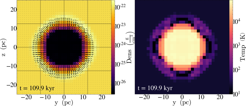
Figure 1: Left: Density plot with overlaid velocity vectors for the supernova injection method of Simpson et. al. 2015. Right: Temperature plot. The kinetic fraction (Eq. [9]) $f_{\rm kin}=0.23$ and $\Delta x=0.8$ pc.

An energy plot for the same run is shown in Fig. 2. Here we note that the transitions between the Sedov-Taylor solution (Draine, 2011a, when the kinetic energy fraction $\sim 0.25$), transition (Haid et al., 2016), and PDS (Draine, 2011a) all appear to match the analytic solutions very well. Also the slope of $E(t)\propto t^{-3/4}$ during the PDS is well recovered.

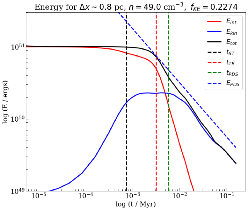
Figure 2: Energy of the supernova shown above. The Sedov-Taylor ($t_{\rm ST}$), thermal ($t_{\rm TR}$), and snow plow ($t_{\rm PDS}$) transition times (Draine, 2011a) are shown as vertical dashed lines, and the analytic form of the energy during the pressure dominated snow plow phase is shown as a blue dashed line above the energy during this phase.

2.3 Winds

In recent years, the general strategy for injecting winds has been to inject mass and velocity in a region around the star to set the kinetic energy of the wind over the timestep (Pelupessy & Portegies Zwart, 2012; Gatto et al., 2017; Rimoldi et al., 2016). This is also the method of Simpson et al. (2015) for supernovae, who use this energy to calculate the momentum for each cell. However, adding momentum to a grid cell that already has mass does not add the same amount of kinetic energy as adding the momentum to an empty cell. Therefore, after adding the momentum of the wind to each cell in the source region, we compute the resulting kinetic energy, and conserve total wind energy by injecting the missing energy as thermal energy into the cell.

Stellar wind feedback is implemented using a method of momentum injection of our own design which was inspired by inverting the method of Simpson et al. (2015). The amount of energy deposited by stellar winds onto the grid is given by the mechanical luminosity

$$L_{w}=\frac{1}{2}\dot{M}v_{w}^{2},$$ (10)

where $\dot{M}$ is the stellar mass loss rate, typically ${10}^{-8}\text{\,}\textrm{M}_{\odot}~{}\mathrm{y}\mathrm{r}^{-1}{10}^{-6}\text{\,}\textrm{M}_{\odot}~{}\mathrm{y}\mathrm{r}^{-1}$ for O and B stars, and $v_{w}$ is the wind terminal velocity, typically $3\text{\times}{10}^{2}\text{\,}\mathrm{k}\mathrm{m}~{}\mathrm{s}^{-1}3\text{\times}{10}^{3}\text{\,}\mathrm{k}\mathrm{m}~{}\mathrm{s}^{-1}$ for the same stars.

We consider the update over time $\Delta t$ of an individual cell with volume $V_{\rm cell}$, density $\rho_{\rm old}$, specific internal energy $e_{\rm intold}$, and velocity $\mathbf{v}_{\rm old}$. We first calculate the overlap fraction $\phi$ between the spherical wind injection region and the cell itself using a $20^{3}$ subgrid of sample points in each cell, following a routine by D. Clarke included in ZEUS-MP (Hayes et al., 2006). This value is normalized to the full volume of the source region (i.e. $\sum_{\rm vol}\phi=1$). The change in density of the cell

$$\delta\rho=\phi\frac{\dot{M}\Delta t}{V_{\rm cell}}.$$ (11)

The stellar wind input kinetic energy for this cell is

$$\delta E_{\rm w}=\phi\frac{L_{w}\Delta t}{V_{\rm cell}}.$$ (12)

The final velocity of the cell can be computed from momentum conservation to be

$$\mathbf{v}=\frac{\delta\rho\mathbf{v}_{\rm w}+\rho_{\rm old}\mathbf{v}_{\rm old}}{\rho_{\rm old}+\delta\rho}<\mathbf{v}_{\rm w}.$$ (13)

The final change in specific kinetic energy is then

$$\delta e_{\rm kin}=\frac{\lvert\mathbf{v}\rvert^{2}}{2}-\frac{\rho_{\rm old}\lvert\mathbf{v}_{\rm old}\rvert^{2}}{2(\rho_{\rm old}+\delta\rho)},$$ (14)

so the specific internal energy of the cell needs to be increased to

$$e_{\rm int}=\frac{\delta E_{\rm w}}{\rho}+e_{\rm intold}\frac{\rho_{\rm old}}{\rho}-\delta e_{\rm kin}.$$ (15)

In determining the radius (e.g. the number of cells) across which to inject the winds, both the physical radius of the wind and the ability of the Cartesian grid to resolve the spherical input are important. Here the analytic solution for a stellar wind bubble is our guide. The radius of the wind termination shock (Weaver et al., 1977, Eq. [12])

$$R_{1}=0.74\left(\frac{\dot{M}}{\rho_{0}}\right)^{\frac{3}{10}}v_{w}^{\frac{1}{10}}t_{w}^{\frac{2}{5}},$$ (16)

where $t_{w}$ is the lifetime of the wind and $\rho_{0}$ is the background density. Within this region the wind will be free streaming. If this radius is resolved by more than a single cell, we directly inject the energy and momentum calculated as above in the resolved region out to a maximum radius of $6\sqrt{3}\ \Delta x$, a radius at which we find spherical winds to be well resolved. If $R_{1}<\Delta x$, we set the radius of the injection region to be $\Delta x$. Note that since the stars are Lagrangian particles not restricted to the cell centers, even wind bubbles smaller than a single cell generally inject not just thermal energy but also momentum and kinetic energy into the grid by straddling cell boundaries.

For each cell within this radius we determine the fractional overlap of the cell with the wind injection region and add that fraction of momentum and thermal energy into the cell, with the momentum and energy evenly distributed throughout the sphere defined by the injection radius. To guarantee that all cells are at maximum resolution in the source region, we add a new criterion that enforces refinement of all blocks that lie within the injection radius of the star.

The mass of hot gas within real stellar wind bubbles is determined by conductive evaporation (Weaver et al., 1977), as well as turbulent mixing, across the contact discontinuity at $R_{\rm C}$ (see Fig. 3) between the hot, rarefied, shocked stellar wind and the dense, radiatively cooled shell. The extra density injected by these mechanisms reduces the temperature in the hot region between $R_{1}$ and $R_{\rm C}$, and thus the sound speed. Capturing this physics exactly is computationally challenging, as conductive evaporation is a diffusive process with Courant timestep $\Delta t_{\rm diff}\propto\Delta x^{2}$. However, the Courant timestep $\Delta t_{\rm C}=C_{\rm CFL}\Delta x/\mbox{max}(v,c_{s})$ is dominated by the high sound speed $c_{s}$ in the hot region. Therefore, we introduce the option to mass load the wind to bring its temperature to the correct order of magnitude. We choose a mass-loaded temperature target $T_{\rm ml}=$$5\text{\times}{10}^{6}\text{\,}\mathrm{K}$ in our simulations, set to lie at the low end of the quasi-stable hot gas phase (McKee & Ostriker, 1977a). We ensure this temperature by reducing the pre-shock velocity of the wind such that the post-shock temperature (Draine, 2011a)

$$T_{s}=$1.38\text{\times}{10}^{7}\text{\,}\mathrm{K}$~{}\left(\frac{v_{w}}{${10}^{3}\text{\,}\mathrm{k}\mathrm{m}~{}\mathrm{s}$^{-1}}\right)^{2}<T_{\rm ml}.$$ (17)

We make up the lost energy by adding to the mass of the wind until we recover the proper wind luminosity. We have found this to be sufficiently hot that the wind bubble in diffuse gas ($n\sim 1$ cm^-3) continues to conserve energy in the shocked gas as expected, while allowing significant gains in the size of the Courant time step.

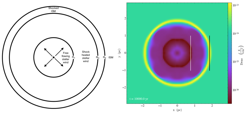
Figure 3: Comparison between Figure 1 of Weaver et al. (1977) and our own test with $\dot{M}=$ ${10}^{-6}\text{\,}\textrm{M}_{\odot}~{}\mathrm{y}\mathrm{r}^{-1}$ and $v=$2\text{\times}{10}^{3}\text{\,}\mathrm{k}\mathrm{m}~{}\mathrm{s}$^{-1}$, at time $t=10^{4}$ yr. The inner white line indicates the analytic solution for the stellar wind termination shock radius $R_{1}$ and the outer black line the solution for the outer shock radius $R_{2}$ from Weaver et al. (1977). Note that the shell has cooled and collapsed at this point, with the distance between the contact discontinuity $R_{c}$ and $R_{2}$ now resolved by at most two cells.

The combination of this radius with the division of kinetic and thermal energy described above leads to bubbles in dense gas primarily injected with thermal energy until the free streaming wind is resolved (and with it the inner boundary of the hot wind bubble), at which point the injection of energy shifts over towards kinetic. This method shows excellent agreement with theoretical predictions for wind bubbles given by Weaver et al. (1977). Comparison between their analytic solution and a plot from our test runs is shown in Figure 3.

To calculate the mass loss rates for our stars we follow Vink et al. (2000) while for the velocities we use the fitting formula of Kudritzki & Puls (2000). These methods include the bi-stability jump in wind strength in late O and early B stars produced by the higher absorption cross section of Fe iii compared to Fe iv (Vink et al., 2000).

2.4 Heating and Cooling

2.4.1 Ultraviolet Radiation Heating

Heating from our stellar sources in the EUV and FUV is calculated by converting the photons to energy fluxes, then applying those fluxes weighted by the probability of an electron of a given energy actually being ejected from an ion or dust grain when it absorbs a photon. For hydrogen ionization this is done by simply differencing the energy of the photon and the ionization potential of hydrogen.

For the background FUV we assume a constant flux of $1.7G_{0}$ and estimate the local visual extinction

$$A_{v}\sim\frac{\lambda_{J}n_{\rm H}}{N_{\rm H}},$$ (18)

where $N_{\rm H}=$1.87\text{\times}{10}^{21}\text{\,}\mathrm{c}\mathrm{m}^{2}$$ and we take the length scale to be the local Jeans length (Jeans, 1902)

$$\lambda_{J}=\left[\pi c_{s}^{2}/(G\rho)\right]^{1/2},$$ (19)

following the methods of Seifried et al. (2011) and Walch et al. (2015). The fraction of FUV radiation that can heat the gas is then $f_{\rm ext}=\exp(-3.5A_{V})$.

For the FUV flux we normalize to the Habing flux $G_{0}$ following Equation (8) to find $G$, and then calculate the heating function per unit volume

$$n_{\rm H}\Gamma_{\rm pe}=n_{\rm H}\epsilon G$$ (20)

where $\epsilon$ is a heating efficiency function. We have implemented several different approximations to this function, including detailed fits from Weingartner & Draine (2001) and Wolfire et al. (2003), as well as a simple adjustable parameter following Joung & Mac Low (2006).

The Weingartner & Draine (2001) efficiency function is given by

$$\frac{\epsilon}{10^{-26}\,$\mathrm{e}\mathrm{r}\mathrm{g}\ \mathrm{s}^{-1}$}=$$ (21)

$$=\frac{7.64+4.52T^{0.132}}{1+$4.37\text{\times}{10}^{-2}$G_{\rm f}^{0.452}\left(1+$5.57\text{\times}{10}^{-3}$G_{\rm f}^{0.675}\right)}.$$

The coefficients are taken from their Table 2, using the case with a ratio of visual extinction to reddening $R_{V}=3.1$, carbon abundance with respect to hydrogen of $b_{c}=6\times 10^{-5}$, distribution A, which minimizes the amount of C and Si in grains, and the stellar radiation field of a B0 star, corresponding to a blackbody with $3\times 10^{4}K$ up to 13.6 eV. The flux factor

$$G_{\rm f}=\frac{G\sqrt{T}}{n_{\rm e}}.$$ (22)

The Wolfire et al. (2003) function is given by

$$\frac{\epsilon}{1.3\times 10^{-24}\,$\mathrm{e}\mathrm{r}\mathrm{g}\ \mathrm{s}^{-1}$}=$$ (23)

$$=\frac{4.9\times 10^{-2}}{1+4.0\times 10^{-3}\left(G_{\rm f}/\phi_{\mathrm{PAH}}\right)^{0.73}}+$$

$$+\frac{3.7\times 10^{-2}\left(T/10^{4}\right)^{0.7}}{1+2.0\times 10^{-4}\left(G_{\rm f}/\phi_{\mathrm{PAH}}\right)},$$

with $\phi_{\mathrm{PAH}}=0.5$ following their assumption. Finally, the simplest assumption is to just follow Joung & Mac Low (2006) and set a constant value of $\epsilon=6.5\times 10^{-26}\,$\mathrm{e}\mathrm{r}\mathrm{g}\ \mathrm{s}^{-1}$$. In the example models analyzed in Paper I and here, we use the Weingartner & Draine (2001) approximation (Eq. [21]).

2.4.2 Dust Temperature

Any photons absorbed that do not eject electrons contribute directly to heating the dust. The dust density is assumed to be a constant 0.01 fraction of the gas density (Draine, 2011a). When solving for the dust temperature we use the radiative cooling rate from Goldsmith (2001), assuming the dust is always optically thin at our densities $n_{\rm H}<${10}^{6}\text{\,}\mathrm{c}\mathrm{m}^{-3}$$, while applying photoelectric heating as previously described. To calculate the dust temperature we use Newton’s root finding algorithm as in Seifried et al. (2011), which generally converges in less than ten steps.

2.4.3 Cosmic Ray Heating

Cosmic ray heating is applied with an ionization rate of $\zeta=${10}^{-17}\text{\,}\mathrm{s}^{-1}$$ and a heating rate of $\Gamma_{\rm cr}/n_{\rm H}=($20\text{\,}\mathrm{e}\mathrm{V}$)\zeta=$3\text{\times}{10}^{-27}\text{\,}\mathrm{e}\mathrm{r}\mathrm{g}\ \mathrm{s}^{-1}$$ as appropriate for the dense regions we are attempting to simulate (Galli & Padovani, 2015).

2.4.4 Gas Cooling

For gas cooling we include contributions from atomic and molecular species as well as dust grains. For the atomic contribution we use the piecewise power law in Joung & Mac Low (2006, Fig. 1), itself derived from equilibrium ionization values given by Sutherland & Dopita (1993). For molecular cooling we use tabulated values from Neufeld et al. (1995) which were originally implemented in FLASH by Seifried et al. (2011), while for dust we use the method of Goldsmith (2001) with the cooling equation for dust from Hollenbach & McKee (1989). Note that dust cooling is also limited to temperatures $T<T_{\rm sputter}$ (see Sect. 2.1.3).

2.4.5 Numerical Solution

To solve the implicit difference equation for the temperature of the gas under all of these heating and cooling sources we have implemented Brent’s 1973 method, which we find to be more accurate and stable than the Euler method used by Joung & Mac Low (2006) and Baczynski et al. (2015). In each cell, all heating $\Gamma_{i}(\epsilon)$ and cooling $\Lambda_{j}(\epsilon)$ rates are combined to find the rate of change of specific internal energy

$$\frac{de}{dt}=\Gamma_{i}(\epsilon)n-\Lambda_{j}(\epsilon)n^{2}.$$ (24)

The cooling rate at the minimum allowed temperature in the simulation (generally $10\text{\,}\mathrm{K}$, but could be as low as the CMB background temperature) is calculated and subtracted from the total cooling rate to set a temperature floor. Then, the difference equation

$$e^{i+1}-e^{i}-\Delta t\frac{de}{dt}=0$$ (25)

is solved for $e^{i+1}$ by the Brent method.

Figure 4 shows the temperature for a cell initially at $T=$ ${10}^{5}\text{\,}\mathrm{K}$ cooling over $10\text{\,}\mathrm{M}\mathrm{y}\mathrm{r}$ using the original Euler method of Joung & Mac Low (2006) and our implicit method, as well as a more expensive Runge-Kutte 4(5) method with local extrapolation (Press, 2007). For a given time step criterion, the implicit method is generally about twice as accurate as the Eulerian method and $\sim 30\%$ faster than the Runge-Kutte method. Given that we call this solver on every iteration of the ray tracing method as we converge to an ionization solution, we have chosen to use the implicit method due to its combination of speed and accuracy.

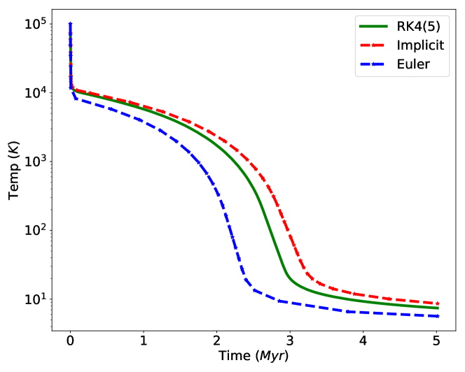
Figure 4: Temperature of a single gas cell with $n_{\rm H}=${10}^{4}\text{\,}\mathrm{c}\mathrm{m}^{-3}$$ initially at ${10}^{5}\text{\,}\mathrm{K}$ as it evolves over $5\text{\,}\mathrm{M}\mathrm{y}\mathrm{r}$ in the presence of a background UV field of $1.69\ G_{0}$ integrated with our three different methods.

2.4.6 Tests

In order for our simulations to resemble the real interstellar medium (ISM) as closely as possible, our heating and cooling solutions should be able to replicate the three-phase ISM (McKee & Ostriker, 1977b; Cox, 2005), where we have equal pressure solutions for a quasi-static hot medium and warm and cold media. Being able to maintain the different thermal phases of the ISM in pressure equilibrium is important generally. It is particularly important for the initial conditions chosen for our proof-of-concept models, since the background medium for some of our clouds is warm neutral medium, while the clouds themselves always consist of cold neutral medium in pressure equilibrium with the background at the initial time.

To test our heating and cooling methods we therefore created a single cell simulation that iterates over hydrogen number densities with $10^{-4}\leq n_{\rm H}\leq${10}^{4}\text{\,}\mathrm{c}\mathrm{m}^{-3}$$, solving for the equilibrium temperature and pressure with Milky Way-like background FUV and cosmic ray values. The results are shown in Figure 5, where the three-phase medium is shown to be stable in our simulations from $P\sim$ $4\text{\times}{10}^{3}\text{\,}\mathrm{K}~{}\mathrm{c}\mathrm{m}^{-3}2\text{\times}{10}^{4}\text{\,}\mathrm{K}~{}\mathrm{c}\mathrm{m}^{-3}$, reproducing similar ranges found in Wolfire et al. (2003, Fig. 7) for the solar neighborhood. Note that we can adjust this range by increasing or decreasing our background FUV, as discussed in Hill et al. (2018), which also uses the atomic cooling model our method is based on.

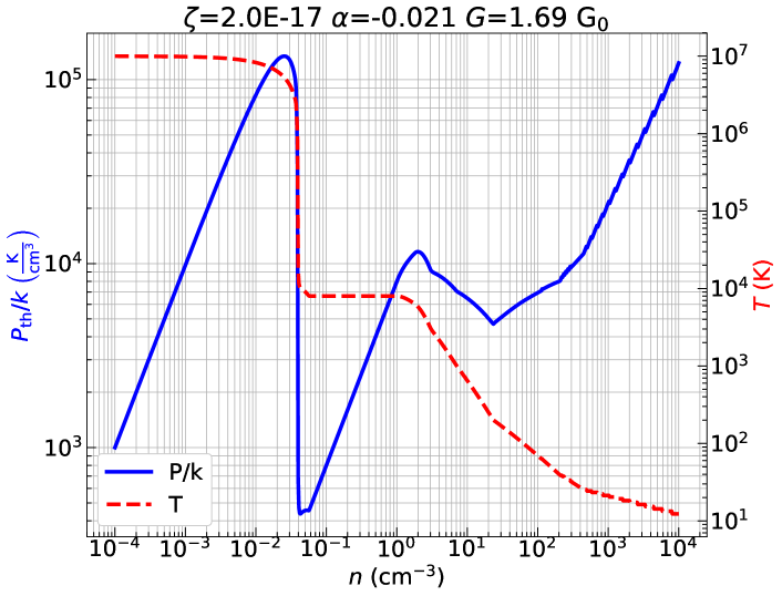
Figure 5: Temperature (blue, solid line) and pressure (red, dashed line) of a single gas cell with $10^{-4}\leq n_{\rm H}\leq 10^{4}\,$\mathrm{c}\mathrm{m}^{-3}$$ evolved until equilibrium in the presence of a background UV flux of $G=1.69\ G_{0}$ and cosmic ray background ionization rate of $\zeta=$2\text{\times}{10}^{-17}\text{\,}\mathrm{s}^{-1}$$ integrated using the implicit method. The two-phase medium occurs for densities of roughly $10^{-1}\leq n_{\rm H}<10^{3}$ cm^-3, and a quasi-static third phase at high temperature and low density is then consistent with the pressure.

3 Example Runs

Table 1: Parameters for each of the four runs described here including cloud mass $M$, radius $R$, and central density $\rho_{c}$, in units of $\rho^{\prime}=2.39\times 10^{-23}\mbox{ g cm}^{-3}$, normalization of the velocity perturbation spectrum $v_{0}$, the number of refinement levels $N_{\rm ref}$, cell size $\Delta x$ at maximum refinement, and the domain size $D$. We further give the total number of stars $N_{s}$ at the final time $t_{\rm end}$, as well as the time the first star formed $t_{\rm sf}$. Note that M3 and M3f used different random turbulent patterns initially, explaining their different values of $t_{\rm sf}$.

Run	$M$ ($\textrm{M}_{\odot}$)	$R$ (pc)	$\rho_{c}/\rho^{\prime}$	$v_{0}$ (km s-1)	$N_{\rm ref}$	$\Delta x$ (pc)	$D$ (pc)	$N_{\rm s}$	$M_{s}$ (M⊙)	$t_{\rm sf}$ (Myr)	$t_{\rm end}$ (Myr)
M3	$10^{3}$	3	46	0.616	8	0.01	10	1100	514	2.86	4.38
M3f	$10^{3}$	3	46	0.616	7	0.02	10	1062	338	2.31	3.90
M3f2	$10^{3}$	5	10	0.616	7	0.01	14	52	43.5	5.22	5.60
M5f	$10^{5}$	50	1.0	1.58	8	0.2	110	1144	501	15.4	17.8

For testing stellar feedback we present four proof-of-concept runs, three of which include radiation, winds and supernova. However, we terminated these runs for cost reasons before any massive star had exploded as a supernova, so we restrict our discussion to radiation and winds. In Table 1 we show the initial cloud properties, grid resolution and time of initial star formation for these runs.

All four simulations use an initial density field that is spherically symmetric and distributed radially as a Gaussian (Bate et al., 1995; Goodwin et al., 2004) with full width at half maximum at the cloud radius $R$. The velocity field is initialized with a turbulent Kolmogorov velocity spectrum $v(k)=v_{0}k^{-5/3}$ from wavenumber $k=2$ to $k=32$ (Wünsch, 2015) for the dense gas, where $k=2\pi/D$ for a simulation domain with side $D$. We note that choosing the initial conditions does determine a good deal about the subsequent evolution (Goodwin et al., 2004; Girichidis et al., 2011). The surrounding medium is initialized with zero velocity and in pressure equilibrium with the cloud gas. Refinement and derefinement are controlled by the Jeans (1902) criterion as described in Federrath et al. (2010). We now describe individual characteristics of these runs.

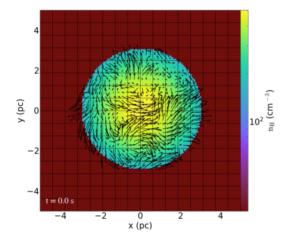
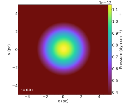
(a)	(b)

Figure 6: Plots showing the initial conditions in (a) H nuclei density and (b) pressure for run M3f. Velocity vectors and initial grid blocks, which each contain $16^{3}$ cells, are annotated on the density plot.

3.1 M3

In this run, which includes no feedback, two subclusters form that subsequently merge. We highlight the merger event in the relevant plots throughout by including a grey shaded box on each plot covering the time of the merger event. This is the only run among our proof-of-concept models that features a merger.

3.2 M3f

In this run several stars form in the main cluster that are massive enough to have ionizing and wind feedback. The growth of an H ii region is initially suppressed by dense gas accretion, creating flickering H ii regions (Peters et al., 2010a, c; De Pree et al., 2014). This continues until the number of massive stars gets large enough for their combined wind and ionization feedback to clear an expanding H ii region around the main cluster, near the end of the run. Around this same time a second cluster forms in the simulation. While the two clusters appear to be falling toward each other, they have yet to merge at the end of the run.

3.3 M3f2

This run starts with the surrounding lower density gas in the warm, neutral phase at $4\text{\times}{10}^{3}\text{\,}\mathrm{K}$, as opposed to the cold phase at roughly $60\text{\,}\mathrm{K}$ in the other two ${10}^{3}\text{\,}\textrm{M}_{\odot}$ runs. Therefore, the surface density is lower than those runs, resulting in slower accretion onto the star forming region. Similarly, feedback is more effective in expelling the gas from the star forming region, since the feedback sees a smaller surface density above it (Grudić et al., 2018). The more effective feedback rapidly shuts down star formation in this run, which therefore only produces 52 stars.

3.4 M5f

In our final run we start with an initial sphere of ${10}^{5}\text{\,}\textrm{M}_{\odot}$ and a radius of $50\text{\,}\mathrm{p}\mathrm{c}$. The gas outside the sphere is initially in the warm ionized phase at $\sim$8\text{\times}{10}^{3}\text{\,}\mathrm{K}$$. Once the gas collapses and begins to form stars, a large central cluster appears, as well as a secondary, smaller cluster. The central cluster rapidly grows until it stochastically forms a $97\text{\,}\textrm{M}_{\odot}$ star, the most massive star formed to date in any simulation we have run.

This star rapidly expels all remaining gas from the central cluster, leaving pillars of gas surrounding the star forming region (see Fig. 7 d) that resemble the Eagle Nebula and similar formations (e.g. Hester et al., 1996; McCaughrean & Andersen, 2002; McLeod et al., 2015).

A difficulty in performing simulations of large clouds from idealized initial density conditions stems from the initial free-fall time for the gas in the Gaussian sphere, which for this run is only $8.6\text{\,}\mathrm{M}\mathrm{y}\mathrm{r}$. Since turbulence decays within a free fall time $t_{\rm ff}$ (Mac Low et al., 1998), the velocity distribution of the gas became quite smooth by the time star formation commenced in this run at $15.4\text{\,}\mathrm{M}\mathrm{y}\mathrm{r}$. Similar concerns were discussed by Krumholz et al. (2012), who noted that this affects both star formation rate and efficiency. Future models of high mass clouds will need to start with more realistic initial conditions that better model the actual assembly of such structures.

Figure 7: Projected number density along the $z$-axis for runs (a) M3 (b) M3f (c) M3f2 and (d) M5f at the last data file from each run. The area of the circles representing stars are proportional to their mass, while the locations of sink particles are shown by white star symbols. Feedback is most effective in run (b) where multiple massive stars with strong feedback have sunk together to the center of the cluster and in (d) due to the $97~{}\textrm{M}_{\odot}$ star in the center of the image.

3.5 Stellar Group Identification

To identify stars as group members within the simulation we used two methods, HOP (Eisenstein & Hut, 1998), which is included in AMUSE, and the Scikit-Learn (Pedregosa et al., 2011) implementation of DBSCAN (Ester et al., 1996; Schubert et al., 2017). HOP determines group membership by the following procedure:

1. Calculate the local density at each particle using its $N_{\rm nn}$ nearest neighbors and the local density gradient at each particle using its $N_{\rm hop}$ nearest neighbors.

2. From each particle, hop to the next particle of the $N_{\rm hop}$ neighbors in the direction of the highest density gradient. Continue until the current particle is the density maximum of the $N_{\rm hop}$ nearest particles.

3. Identify this particle as a group core particle, with this particle’s density as the group peak density $\rho_{\rm peak}$. All particles in the path of hops leading to this particle are added to this group as members. Repeat this process until all particles are in groups.

4. Identify particles that reside on the boundary between two groups by identifying particles where one of its $N_{\rm merge}$ nearest neighbors belongs to a different group. Record the density at these locations as the saddle density, $\rho_{\rm saddle}$, calculated as the average density between the two boundary particles.

5. Merge any groups where $\rho_{\rm saddle}$ is either greater than an absolute saddle density $\delta_{\rm saddle}$, or whose ratio of saddle to peak densities is less than a given relative saddle density factor threshold $f_{\rm saddle}$. In mergers the group with the lower peak density $\rho_{\rm peak}$ is merged into the group with the higher peak density.

6. Remove any group whose peak density is lower than the outer threshold density $\delta_{\rm outer}$.

For physical parameters in HOP we use an outer stellar mass density threshold $\delta_{\rm outer}=$1\text{\,}\textrm{M}_{\odot}~{}\mathrm{p}\mathrm{c}^{-3}$$, an order of magnitude lower than the average stellar density of an open cluster and an order of magnitude greater than the stellar density of the Milky Way (Binney & Tremaine, 2011). For the peak density we use $\delta_{\rm peak}=3\delta_{\rm outer}$ as suggested in the original paper. For the saddle density we use a relative saddle density threshold, where the boundary saddle density is compared to the minimum peak density of the two groups, defined by

$$D=\frac{\delta_{\rm saddle}}{{\rm min}\left(\delta_{\rm peak,1};\delta_{\rm peak,2}\right)}.$$ (26)

If $D<f_{\rm saddle}$, where $f_{\rm saddle}$ is the saddle density threshold factor, the two groups are merged. For our analysis here we set $f_{\rm saddle}=0.5$, slightly more aggressively merging groups than the default value of 0.8. The values ($N_{\rm merge}$, $N_{\rm hop}$, $N_{\rm nn}$) = (4,16,64), again as suggested in Eisenstein & Hut (1998).

DBSCAN on the other hand determines group membership using a simpler procedure:

1. Any particle with at least $N_{\rm min}$ neighbors within a distance $\xi$ is considered a core particle.

2. Any particle that is within distance $\xi$ of at least one core particle, but has fewer than $N_{\rm min}$ neighbors, is considered a boundary particle.

3. All connected core and boundary particles define a group.

4. Any other particles are defined as noise.

For DBSCAN we set $N_{\rm min}=16$ for a core particle and we calculate $\xi$, the maximum neighboring particle separation, to match our physical parameters in HOP. Assuming an average stellar mass of $M_{\rm avg}=$0.56\text{\,}\textrm{M}_{\odot}$$ for the initial mass function (IMF) of Kroupa (2001) and using a stellar density of $\rho_{\rm bg}=$1\text{\,}\textrm{M}_{\odot}~{}\mathrm{p}\mathrm{c}^{-3}$$ we compute

$$\xi=\left(\rho_{\rm bg}/M_{\rm avg}\right)^{-1/3}=$0.84\text{\,}\mathrm{p}\mathrm{c}$,$$ (27)

which we used for the one run we analyzed with DBSCAN here, M5f.

Generally we prefer HOP due to its physically motivated thresholds, particularly its ability to compare the relative saddle density between two groups to the minimum peak density of the groups themselves to determine if the two groups should be merged. However it was more practical to use the simpler DBSCAN technique for our largest data set. As with any group-finding numerical technique, both methods struggle to disentangle whether one or two groups exist just before the point of merger. However, we only have one run that experiences a merger of two nearly equal sized groups, while others are either well separated or have mergers where one group is clearly the more massive and dominates the potential. As a check, we examined several times during M5f and verified that we found similar results with HOP and DBSCAN. Both methods provide similar and consistent grouping results when compared on the same data over multiple grouping computations, with an agreement of $>95\%$ on cluster members.

4 Results

4.1 Star Formation

The star formation rate (SFR) as a function of time in our simulations is shown in Figure 8. The data shown as blue points is initially calculated by a second-order central difference of the stellar masses every timestep (as little as 100 yr), which are generally quite noisy. We also show the result of using a Savitzky-Golay (1964) filter convolved with a window size of 51 and fit to a third-order polynomial to smooth the data before we take the derivative (black lines). We use this filter on all data hereafter presented with open circles, representing the data taken directly from the simulation, accompanied by line plots, which show the result of the smoothing. For the SFR, we further smooth with a Gaussian filter with 3 kyr variance.

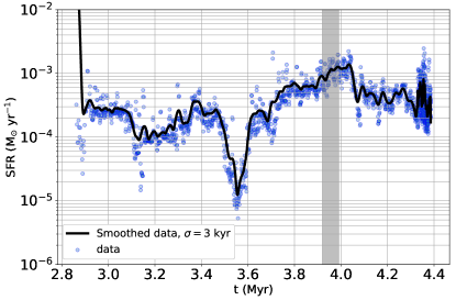
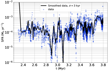
(a)	(b)
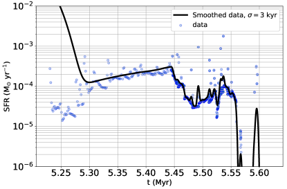
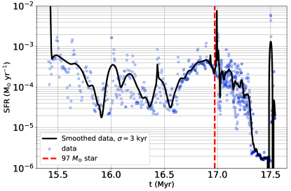
(c)	(d)

Figure 8: Star formation rates for runs (a) M3 (b) M3f (c) M3f2 and (d) M5f. Blue dots show data points every timestep (which during feedback can be as small as 100 yr), while black line shows the SFR smoothed with a Gaussian filter with $\sigma=$3\text{\,}\mathrm{k}\mathrm{y}\mathrm{r}$$. The grey shaded area in (a) shows time of subgroup merger, while the red dashed vertical line in (d) shows the formation of $A_{*}$, the $97\text{\,}\textrm{M}_{\odot}$ star.

In the M3 run without feedback, the SFR generally stays high, only briefly decreasing due to a strong interaction in the main group that placed many of the massive stars on wide orbits and slowed the overall accretion rate of the region. In the first run with feedback, M3f, the data are much noisier due to the flickering H ii regions (see Sect. 3.2), which heat the gas briefly and inject turbulence, but never provide enough outward momentum to the nearby gas to eject it nor ionize enough material to prevent it from cooling again. The lower surface density run M3f2 shows relatively stable star formation until the first massive stars appear at $5.45\text{\,}\mathrm{M}\mathrm{y}\mathrm{r}$. Their feedback breaks up the filament in which stars are forming, but cannot entirely disperse the dense gas in the region. This allows star formation to continue for another ${10}^{4}\text{\,}\mathrm{y}\mathrm{r}$ until an interaction between two massive stars expels one far enough out of the center of the group for a second H ii region to form and expand out of the star-forming region. In run M5f the SFR shows large variations as filaments form and intersect in the first megayear and two separate groups form. At around $17\text{\,}\mathrm{M}\mathrm{y}\mathrm{r}$, a $97\text{\,}\textrm{M}_{\odot}$ star forms in the more massive group, emitting radiation and winds that travel throughout the simulation domain, although star formation continues both near and far from the star for another $\sim$3\text{\times}{10}^{5}\text{\,}\mathrm{y}\mathrm{r}$$ before effectively terminating.

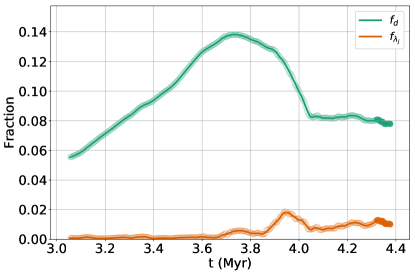
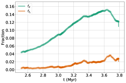
(a)	(b)
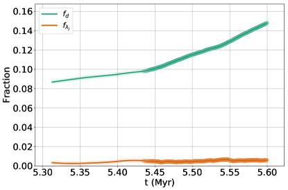
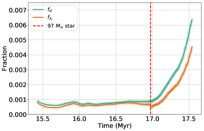
(c)	(d)

Figure 9: Total dense and Jeans unstable gas fractions for runs (a) M3 (b) M3f (c) M3f2 and (d) M5f.

The amount of gas available to form stars is presented in Figure 9 where we show both the fraction (by mass) of dense gas (for which $n_{\rm H}>${10}^{4}\text{\,}\mathrm{c}\mathrm{m}^{-3}$$, the limit generally considered for gas to be star forming; Lada et al., 2010) and the fraction of Jeans unstable gas. For all the runs except M5f, the amount of Jeans unstable gas is much smaller, generally by a factor of two or more, than the amount of dense gas. This agrees with results found by Dale et al. (2015a), who concluded that dense gas is a necessary but not sufficient condition for star formation. Also in agrement with Dale et al. (2015a) is our finding that effective stellar feedback, which occurs in runs M3f2 and M5f, actually produces more dense gas, rather than reducing it. Only in run M5f does feedback also seem to increase the amount of Jeans unstable gas, thereby leading to increased star formation near the center of feedback. The difference between the feedback in M3f2 and M5f is that the stellar wind from the extremely massive star in M5f can sweep up a shell dense enough to trap its own H ii region, allowing some triggered star formation in the shell (see Sect. 4.4).

4.2 Stellar Group Structural Evolution

We next examine the effectiveness, or lack thereof, of stellar feedback on the evolution of the groups that contain massive stars. Given the expectation that 90% of all clusters are disrupted (Lada & Lada, 2003), presumably by gas expulsion, we might expect any feedback that completely ejects the natal gas to destroy the cluster it formed from by removing the dense gas potential helping to bind the cluster (e.g. Tutukov, 1978; Elmegreen, 1983; Parmentier et al., 2008; Goodwin, 2009; Rahner et al., 2017, 2019).

4.2.1 Energetics

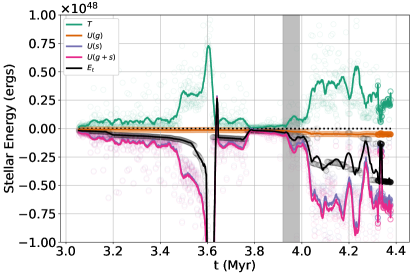
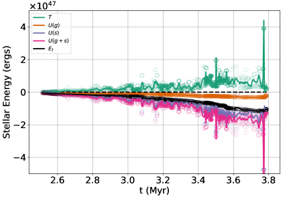
(a)	(b)
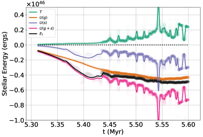
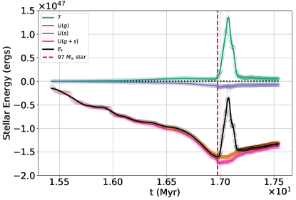
(c)	(d)

Figure 10: Total energy of the stars $E_{\rm t}$ in the main stellar groups for runs (a) M3 (b) M3f (c) M3f2 and (d) M5f, showing that they all end bound. Also shown are stellar kinetic energy $T$, potential energy due to gas $U(g)$ and stars $U(s)$, and their sum $U(g+s)$. The grey shaded area in (a) shows time of subgroup merger, while the red dashed vertical line in (d) shows the formation of $A_{*}$, the $97\text{\,}\textrm{M}_{\odot}$ star. Varying energy ranges come from varying compactness of the main group in each case.

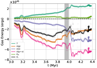
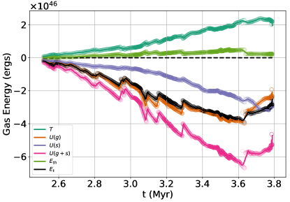
(a)	(b)
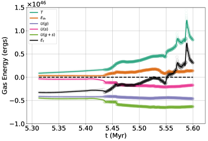
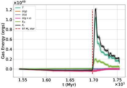
(c)	(d)

Figure 11: Total energy of the gas $E_{\rm t}$ for the main groups in runs (a) M3 (b) M3f (c) M3f2 and (d) M5f. Also shown are gas kinetic energy $T$, thermal energy $E_{\rm th}$, and potential energy due to gas $U(g)$ and stars $U(s)$, and their sum $U(g+s)$. The grey shaded area in (a) shows time of subgroup merger, while the red dashed vertical line in (d) shows the formation of $A_{*}$, the $97\text{\,}\textrm{M}_{\odot}$ star.

Figures 10 and 11 show the energy in stars and gas respectively contained within the radius of the main group for each run. These figures show that only runs M3f2 and M5f actually eject their natal gas, when their total gas energy becomes positive. However both stellar groups remain bound with negative total energies after the gas is removed, identifying them as true clusters.

This is further confirmed by looking at the virial ratios $\alpha=2T/U$ of the gas and stars in these groups (Fig. 12), where the group as a whole appears briefly unbound during the time that some of the outer stars escape following gas ejection, but the overall group survives and returns to a bound virial ratio in both cases. Indeed, the group in run M5f is subvirial at the time of the final snapshot, and the other three groups are close to being virialized, regardless of the current state of the gas in the region defined by the group. We do see mass segregation in our runs, as detailed below, which might contribute to their being observed as supervirial, something we will examine in more detail in future work. Our groups appear likely to survive gas ejection, and mass segregation may assist in their survival, since increasing stellar to gas density ratios increases the likelihood of surviving the gas ejection stage (Kruijssen et al., 2012).

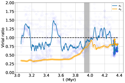
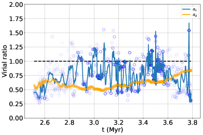
(a)	(b)
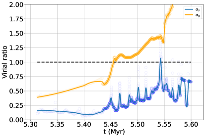
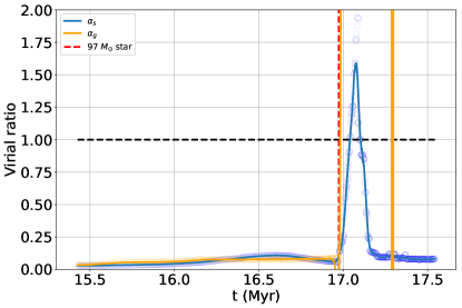
(c)	(d)

Figure 12: Virial ratios for the stars $\alpha_{s}$ and gas $\alpha_{g}$ in the main groups for runs (a) M3 (b) M3f (c) M3f2 and (d) M5f. The grey shaded area in (a) shows time of subgroup merger, while the red dashed vertical line in (d) shows the formation of $A_{*}$, the $97\text{\,}\textrm{M}_{\odot}$ star.

4.2.2 Mass

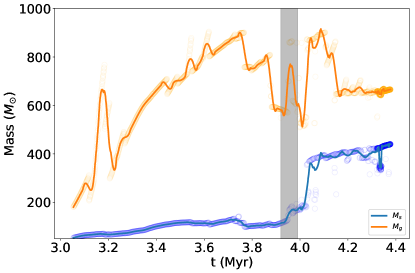
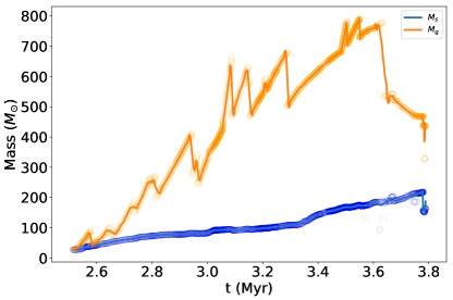
(a)	(b)
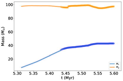
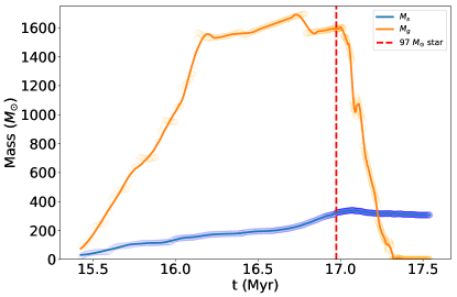
(c)	(d)

Figure 13: Total mass in stars and gas in the main groups for runs (a) M3 (b) M3f (c) M3f2 and (d) M5f. The grey shaded area in (a) shows time of subgroup merger, while the red dashed vertical line in (d) shows the formation of $A_{*}$, the $97\text{\,}\textrm{M}_{\odot}$ star.

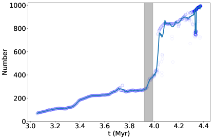
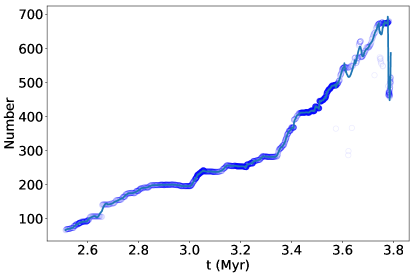
(a)	(b)
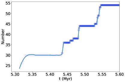
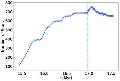
(c)	(d)

Figure 14: Total number of stars in the main groups for runs (a) M3 (b) M3f (c) M3f2 and (d) M5f. The grey shaded area in (a) shows time of subgroup merger, while the red dashed vertical line in (d) shows the formation of $A_{*}$, the $97\text{\,}\textrm{M}_{\odot}$ star.

Figure 13 shows that the mass in gas dominates the mass in all the groups for most of their evolution, only being driven completely out of the group under the intense feedback of M5f’s massive star. Even in M3f2, where the gas actually has positive energy, it has yet to be driven from the group entirely. Indeed, dense gas is growing in the group (Fig. 9 c) as it continues to fall in from the filament and build up along the edge of the H ii region. This infall itself may lead to more star formation, although at the end of the run there has been no similar increase in the amount of Jeans unstable gas, and the total number of stars in the group has been steady for the last $5\text{\times}{10}^{4}\text{\,}\mathrm{y}\mathrm{r}$, as shown in Figure 14. This is similar to our other ${10}^{3}\text{\,}\textrm{M}_{\odot}$ simulation M3f, where feedback near the main group during the previous ${10}^{5}\text{\,}\mathrm{y}\mathrm{r}$ has also stabilized the number of stars. In M5f, feedback eventually leads to the loss of some of the least bound stars in the main group as the gas is ejected, shown by the correlation in the drop in gas mass with the decline in the number of stars in the group.

4.2.3 Radius

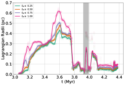
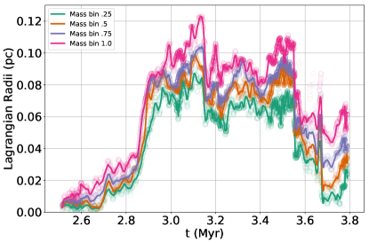
(a)	(b)
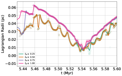
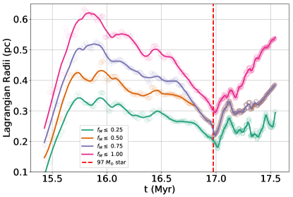
(c)	(d)

Figure 15: Lagrangian radii of all the stars in the main groups for runs (a) M3 (b) M3f (c) M3f2 and (d) M5f. The grey shaded area in (a) shows time of subgroup merger, while the red dashed vertical line in (d) shows the formation of $A_{*}$, the $97\text{\,}\textrm{M}_{\odot}$ star.

In Figure 15 we show the Lagrangian radii for evenly spaced mass bins. In M3 (Fig. 15a), lacking feedback, the group radius drops, aside from a brief bounce when two subgroups merge (grey bar). Gas ejection leading to loss of the least bound stars can be seen in the fast rate of growth of the Lagrangian radii of the central groups for the two runs in which feedback expelled significant amounts of gas: M3f2 (Fig. 15c), and M5 (Fig. 15d). In M5f, the 25% Lagrangian radius of the group only grows by $\sim$33–50%, but the the outer (100%) and half-mass (50%) radii almost double after the onset of stellar feedback.

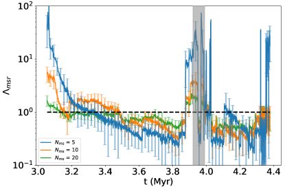
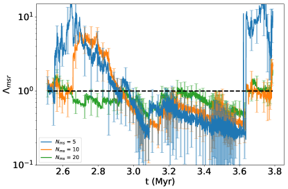
(a)	(b)
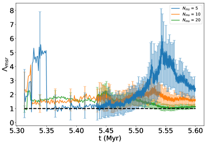
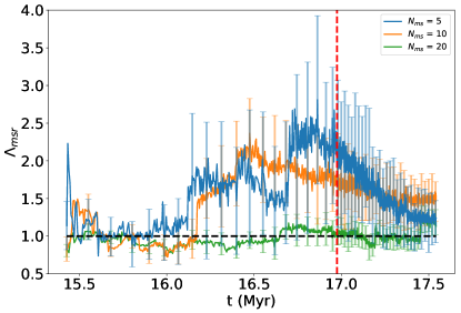
(c)	(d)

Figure 16: Mass segregation ratio $\Lambda_{\rm msr}$ (Eq. 28) for all the stars in the main groups for runs (a) M3 (b) M3f (c) M3f2 and (d) M5f. Mass segregation produces $\Lambda_{\rm msr}>1$. The grey band shows the merger of the two subgroups in M3, while the red, dashed line shows the formation of $A_{*}$.

4.3 Mass Segregation

Next we consider the mass segregation of the groups formed in our simulations. Several methods exist to quantify mass segregation, including looking at the half-mass radii $R_{\rm hm}$ of different mass bins in the group (McMillan et al., 2007, 2015), the mean or median radius of a subset of massive stars (Bonnell & Davies, 1998), and calculating the Gini coefficient of the group (Converse & Stahler, 2008; Pelupessy & Portegies Zwart, 2012).

Allison et al. (2009) pointed out several issues with these methods of computing mass segregation, including how binning can affect the results, the reliance on properly finding the group center, and difficulty in comparison to observations. They presented a new method, based on calculations of $N_{\rm random}$ minimum spanning trees (MSTs) of the group and the MST of the $N_{\rm ms}$ most massive stars contained in the same group as a model independent way of determining the amount of mass segregation. They compared the ratios of the norm of lengths of the random trees, $\langle l_{\rm norm}\rangle$, to the length of the massive star tree, $l_{\rm ms}$, to obtain the mass segregation ratio

$$\Lambda_{\rm msr}=\frac{\langle l_{\rm norm}\rangle}{l_{\rm ms}}\pm\frac{\sigma_{\rm norm}}{l_{\rm ms}},$$ (28)

where $\Lambda_{\rm msr}>1$ indicates mass segregation in the group.

This method is independent of any determination of the group center, always returns the same tree lengths (even if the tree is drawn in a different order), and is simple to implement in both two and three dimensions. Further, since the number of random trees calculated provides a standard deviation of tree length, error for the calculations are straight forward to obtain. We show our calculated values of the three-dimensional value of $\Lambda_{\rm msr}$ in Figure 16 using $N_{\rm ms}=\{5,10,20\}$ and 50 random samples drawn from each group for the comparison trees. We only start tracking groups once they reach 64 stars in size, with the exception of M3f2 where we start following the group at 24 stars.

Two points can be made with this data. First, all of our runs become mass segregated at early times. This presumably occurs because our groups of $N$ stars, with initially short crossing times $t_{\rm cr}=R_{\rm hm}/\sigma_{v}$, have likewise short half-mass relaxation times (Binney & Tremaine, 2011) $t_{r}=0.1Nt_{\rm cr}/\ln N$. The wide range in stellar masses then accelerates the dynamical evolution of the group to a fraction of the half-mass relaxation time scale $t_{\rm seg}\sim\left(\langle m\rangle/\langle m_{\rm hm}\rangle\right)t_{r}$, where $\langle m\rangle$ and $\langle m_{\rm hm}\rangle$ are the mean mass of all and of the high mass stars respectively (Portegies Zwart & McMillan, 2002). The clumpiness of the stellar distribution helps to preserve this primordial mass segregation throughout the assembly of more massive stellar conglomerates, as was predicted by McMillan et al. (2007) from simulations of small merging subgroups.

Second, feedback seems to be correlated with mass segregation in all of the runs including it. We attribute this to gas expulsion having a stronger effect on low mass, loosely bound stars, causing their orbital radii and kinetic energy to increase more than massive stars and leading naturally to an increase in mass segregation even as the whole group expands. Also, all runs that experience significant mass segregation sustain that segregation over their ten most massive stars (Fig. 16c and d), even if the five most massive stars have strong interactions that reduce their ratio $\Lambda_{\rm msr}$. This supports the view (e.g. Girichidis et al., 2012b, a) that subgroups will start more mass segregated than dynamics alone can account for if they can survive the ejection of their natal gas, as seen in many observations of young stellar groups (Hillenbrand & Hartmann, 1998; de Grijs et al., 2002; Gouliermis et al., 2004; Converse & Stahler, 2008).

4.4 Triggered Star Formation

A modest level of triggered star formation has been seen both observationally (Thompson et al., 2012; Liu et al., 2017) and numerically (Dale et al., 2012b; González-Samaniego & Vazquez-Semadeni, 2020), although some care must be exercised in observations since the time evolution of the system is not available as it is in simulations, making it difficult to disentangle triggered star formation from formation that would have otherwise occurred naturally due to gravitational collapse (Dale et al., 2015b). Dale et al. (2007) and Dale et al. (2015b) divide triggering into two categories; weak triggering where star formation that would already occur due to normal collapse is accelerated, but without increasing either the overall star formation efficiency or the number of stars created; and strong triggering where collapse is induced in previously stable gas that increases the total star formation efficiency, the number of stars, or both.

Apparent triggered star formation occurs in run M5f, which has the strongest feedback. At the time of formation of the $97\text{\,}\textrm{M}_{\odot}$ star (hereafter referred to as $A_{*}$) in the main group, there are three star-forming sinks present. The first sink (sink # 56) is the one that actually forms $A_{*}$, and its accretion immediately shuts down. The other two sinks (# 55 and 57) continue accreting gas for another 0.3 Myr from gravitationally unstable regions in the swept up shell driven by the stellar wind from $A_{*}$ (Fig. 17). This appears to be a case of triggering maintaining the global star formation rate temporarily (see Fig. 8 d) even in the presence of strong negative feedback.

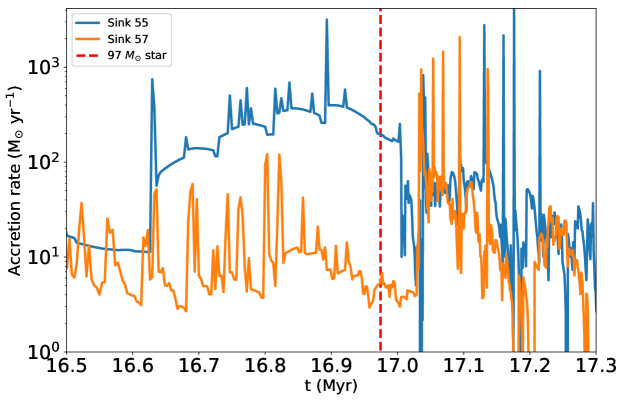
Figure 17: The individual mass accretion rates for the two sinks ejected from the main group due to feedback. The grey shaded area in (a) shows time of subgroup merger, while the red dashed vertical line in (d) shows the formation of $A_{*}$, the $97\text{\,}\textrm{M}_{\odot}$ star.

In the case of sink 55, star formation was already proceeding at a vigorous rate before $A_{*}$ appeared. Therefore this cannot be considered even weakly triggered star formation, however it seems that the intense feedback was unable to do more than briefly slow the production of stars for about $10^{4}$ yr before the sink returned to producing stars at a rate exceeding $4\text{\times}{10}^{-5}\text{\,}\textrm{M}_{\odot}\mathrm{y}\mathrm{r}^{-1}$. In the case of sink 57, though, star formation was at less than $1\text{\times}{10}^{-5}\text{\,}\textrm{M}_{\odot}\ \mathrm{y}\mathrm{r}^{-1}$ when the stellar wind bubble compressed gas in which the sink was embedded. Once this occurred, the rate of star formation grew rapidly. For this to be considered triggered star formation, we should also be able to observe an increase in both the amount of dense gas and Jeans unstable gas in the region surrounding the group occurring as the feedback impacts the region. We show that this increase indeed occurs in Figure 9 (d).

During their ejection, both sinks reached peak speeds of $\sim$30\text{\,}\mathrm{k}\mathrm{m}~{}\mathrm{s}$^{-1}$ with respect to the group center as they followed the expanding gas driven by feedback. This velocity is noteworthy, since it defines the boundary velocity for massive O and B stars that are considered runaway stars (Gies & Bolton, 1986). Generally the production of OB runaways has been considered the result of kicks from a binary partner that goes supernova (Blaauw, 1961; Portegies Zwart, 2000) or due to dynamical interactions with binaries (Leonard & Duncan, 1988; Fujii & Portegies Zwart, 2011). However since our sinks (and therefore also the gas they accrete) reach velocities comparable to that of OB runaways, triggered star formation in our simulation shows a third, and not previously considered, method for producing OB runaways. In this case we produced many lower mass stars, but the total mass produced by the two sinks during this time was over $30\text{\,}\textrm{M}_{\odot}$, therefore the lack of formation of an OB star was simply due to the random selection of our star formation method.

The high gas velocity is clearly connected to the feedback of $A_{*}$, but which physical process contributes the most? The radius and velocity of the D-type front are Spitzer (1978)

$$R = R_{\rm St}\left(1+\frac{7}{4}\frac{c_{s}t}{R_{\rm St}}\right)^{-3/4},$$ (29)

$$\frac{dR}{dt} = c_{s}\left(\frac{R}{R_{\rm St}}\right)^{-3/4},$$ (30)

The velocity of the D front has a maximum value of $v_{\rm d}\sim$15\text{\,}\mathrm{k}\mathrm{m}~{}\mathrm{s}$^{-1}$, too slow for our gas, ruling out compression by radiation. Note this also likely rules out radiation driven implosion (Sandford et al., 1982) as a primary trigger. We also considered a champagne flow as a possible method of driving the gas velocities, but as shown in Bodenheimer et al. (1979) and similar to the case of radiation driven implosion, champagne flows only accelerate the lower density gas to high velocities. Even in their case (5), where they allowed a D-type front to move past a small dense cloud, the dense gas was compressed but the dense gas velocities never exceeded $8\text{\,}\mathrm{k}\mathrm{m}~{}\mathrm{s}$^-1.

This leaves the effect of the winds as the main factor accelerating the gas flow. Normally, the wind bubble would evolve while trapped within the H ii region (Weaver et al., 1977). This means for moderately massive O stars the H ii region dominates the dynamics, since the D-type front strikes the ambient gas first (McKee et al., 1984). However in the case of winds moving rapidly into a region of dense gas the H ii regions can become trapped within the wind shells (van Buren et al., 1990; Mac Low et al., 1991). To calculate the speed of the shell from the wind, we obtained the luminosity and temperature of $A_{*}$ using SeBa and then calculated the wind luminosity using our stellar wind code as described in Sect. 2.3, finding $L_{w}=$2.47\text{\times}{10}^{37}\text{\,}\mathrm{e}\mathrm{r}\mathrm{g}$$. The shell velocity of a stellar wind bubble in a uniform medium is (Weaver et al., 1977)

$$V_{2}(t)=16n_{o}^{-1/5}L_{36}^{1/5}t_{6}^{-2/5}~{}$\mathrm{k}\mathrm{m}~{}\mathrm{s}$^{-1},$$ (31)

with $n_{o}=${10}^{3}\text{\,}\mathrm{c}\mathrm{m}^{-3}$$ to find the wind shell velocity at the peak time of the sink velocities, which is $\sim$3\text{\times}{10}^{4}\text{\,}\mathrm{y}\mathrm{r}$$ after the formation of $A_{*}$. This gives us a shell velocity of $V_{2}=$31\text{\,}\mathrm{k}\mathrm{m}~{}\mathrm{s}$^{-1}$, consistent with the maximum sink velocity of $30\text{\,}\mathrm{k}\mathrm{m}~{}\mathrm{s}$^-1.

Eventually all the star forming filaments that are in close proximity to the main group are disrupted by the feedback of $A_{*}$. At this point ($\sim$17.3\text{\,}\mathrm{M}\mathrm{y}\mathrm{r}$$) the overall star formation rate rapidly drops, as all gas in the region becomes warm, low density H ii gas or hot wind shocked gas. Some small amount of star formation still occurs in a smaller secondary group containing sink # 22, but formation here is slow due to the overall smaller fraction of dense gas present in the group, as shown in Figure 18.

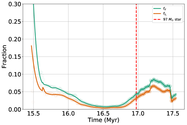
Figure 18: Fractions of dense ($n_{\rm H}>${10}^{4}\text{\,}\mathrm{c}\mathrm{m}^{-3}$$) and Jeans unstable gas in the region defined by group 2. The grey shaded area in (a) shows time of subgroup merger, while the red dashed vertical line in (d) shows the formation of $A_{*}$, the $97\text{\,}\textrm{M}_{\odot}$ star.

5 Summary

This paper describes the implementation of stellar feedback methods in the Torch software package, which incorporates FLASH into the AMUSE software framework (Paper I). Our implementations reproduce standard benchmarks for ionizing radiation, stellar winds, and supernovae. We also include heating from cosmic rays and non-ionizing radiation from both individual stars and the galactic background and radiative cooling from both gas in collisional equilibrium ionization and dust. The implementation of feedback in the Torch package allows its use to model the formation and early evolution of star clusters by combining magnetohydrodynamics using FLASH, collisional N-body dynamics using ph4, binary and higher-order multiple dynamics using multiples, and stellar evolution using SeBa, with the stellar feedback described here.

We have begun to use this framework to study newly formed stellar groups and clusters. We here report on four proof-of-concept simulations with initial gas masses of either $10^{3}\,\textrm{M}_{\odot}$ or $10^{5}\,\textrm{M}_{\odot}$.

Our four models lead to the following tentative conclusions:

1. Stellar feedback can effectively terminate star formation in the region around a stellar group (Sect. 4.1). The details of cloud structure do matter, however, both for the overall star formation rate and because dense shells swept up by feedback can trigger small amounts of additional star formation.

2. Stellar feedback tends to increase the amount of dense gas present in the star forming region, agreeing with Dale et al. (2015a). Contrary to them, however, we do find a case in which feedback even increases the amount of Jeans unstable gas.

3. Our stellar groups generally form subvirial and end marginally virialized (Sect. 4.2.1). Both groups that ejected their gas (M3f and M5f) went through a period of supervirial expansion but ended subvirial, even while they continue to expand.

4. Feedback results in the ejection of gas from our groups, but did not disrupt any of the stellar groups created in the runs presented here, although the least bound stars were lost (Sects. 4.2.2 and 4.2.3).

5. Our stellar groups quickly become mass segregated (Sect. 4.3). Feedback-driven gas removal further stratifies the stars according to their current binding energy. After expulsion of their gas, the groups remain mass segregated, consistent with observations.

References

- Allison et al. (2009) Allison, R. J., Goodwin, S. P., Parker, R. J., et al. 2009, MNRAS, 395, 1449, doi: 10.1111/j.1365-2966.2009.14508.x
- Arthur et al. (2004) Arthur, S. J., Kurtz, S. E., Franco, J., & Albarrán, M. Y. 2004, ApJ, 608, 282, doi: 10.1086/386366
- Baczynski et al. (2015) Baczynski, C., Glover, S. C. O., & Klessen, R. S. 2015, MNRAS, 454, 380, doi: 10.1093/mnras/stv1906
- Bate et al. (1995) Bate, M. R., Bonnell, I. A., & Price, N. M. 1995, MNRAS, 277, 362
- Baumgardt & Kroupa (2007) Baumgardt, H., & Kroupa, P. 2007, MNRAS, 380, 1589, doi: 10.1111/j.1365-2966.2007.12209.x
- Binney & Tremaine (2011) Binney, J., & Tremaine, S. 2011, Galactic Dynamics: (Second Edition), Princeton Series in Astrophysics (Princeton, NJ: Princeton University Press). https://books.google.com/books?id=6mF4CKxlbLsC
- Blaauw (1961) Blaauw, A. 1961, Bulletin of the Astronomical Institutes of the Netherlands, 15, 265
- Bodenheimer et al. (1979) Bodenheimer, P., Tenorio-Tagle, G., & Yorke, H. W. 1979, ApJ, 233, 85, doi: 10.1086/157368
- Bonnell & Davies (1998) Bonnell, I. A., & Davies, M. B. 1998, MNRAS, 295, 691, doi: 10.1046/j.1365-8711.1998.01372.x
- Brent (1973) Brent, R. 1973, Algorithms for Minimization Without Derivatives, Dover Books on Mathematics (Mineola, NY: Dover Publications). https://books.google.com/books?id=FR_RgSsC42EC
- Castor et al. (1975) Castor, J., McCray, R., & Weaver, R. 1975, ApJ, 200, L107
- Converse & Stahler (2008) Converse, J. M., & Stahler, S. W. 2008, ApJ, 678, 431, doi: 10.1086/529431
- Cox (2005) Cox, D. P. 2005, Annual Review of Astronomy and Astrophysics, 43, 337, doi: 10.1146/annurev.astro.43.072103.150615
- Dale et al. (2007) Dale, J. E., Clark, P. C., & Bonnell, I. A. 2007, MNRAS, 377, 535, doi: 10.1111/j.1365-2966.2007.11515.x
- Dale et al. (2012a) Dale, J. E., Ercolano, B., & Bonnell, I. A. 2012a, MNRAS, 424, 377, doi: 10.1111/j.1365-2966.2012.21205.x
- Dale et al. (2012b) —. 2012b, MNRAS, 427, 2852, doi: 10.1111/j.1365-2966.2012.22104.x
- Dale et al. (2013a) —. 2013a, MNRAS, 430, 234, doi: 10.1093/mnras/sts592
- Dale et al. (2015a) —. 2015a, MNRAS, 451, 987, doi: 10.1093/mnras/stv913
- Dale et al. (2015b) Dale, J. E., Haworth, T. J., & Bressert, E. 2015b, MNRAS, 450, 1199, doi: 10.1093/mnras/stv396
- Dale et al. (2013b) Dale, J. E., Ngoumou, J., Ercolano, B., & Bonnell, I. A. 2013b, MNRAS, 436, 3430, doi: 10.1093/mnras/stt1822
- Dale et al. (2014) —. 2014, MNRAS, 442, 694
- de Grijs et al. (2002) de Grijs, R., Gilmore, G. F., Johnson, R. A., & Mackey, A. D. 2002, MNRAS, 331, 245, doi: 10.1046/j.1365-8711.2002.05218.x
- De Pree et al. (2014) De Pree, C. G., Peters, T., Mac Low, M.-M., et al. 2014, ApJ, 781, L36
- Draine (2011a) Draine, B. 2011a, Physics of the Interstellar and Intergalactic Medium, Princeton Series in Astrophysics (Princeton, NJ: Princeton University Press). http://books.google.com/books?id=FycJvKHyiwsC
- Draine (2003) Draine, B. T. 2003, ARA&A, 41, 241, doi: 10.1146/annurev.astro.41.011802.094840
- Draine (2011b) Draine, B. T. 2011b, ApJ, 732, 100, doi: 10.1088/0004-637X/732/2/100
- Eisenstein & Hut (1998) Eisenstein, D. J., & Hut, P. 1998, ApJ, 498, 137, doi: 10.1086/305535
- Elmegreen (1983) Elmegreen, B. G. 1983, MNRAS, 203, 1011, doi: 10.1093/mnras/203.4.1011
- Ester et al. (1996) Ester, M., Kriegel, H.-P., Sander, J., & Xu, X. 1996, in Proc. Second Knowledge Discovery and Data Mining Conf. (AAAI Press), 226–231
- Federrath et al. (2010) Federrath, C., Banerjee, R., Clark, P. C., & Klessen, R. S. 2010, ApJ, 713, 269
- Fleck et al. (2006) Fleck, J. J., Boily, C. M., Lançon, A., & Deiters, S. 2006, MNRAS, 369, 1392, doi: 10.1111/j.1365-2966.2006.10390.x
- Fryxell et al. (2000) Fryxell, B., Olson, K., Ricker, P., et al. 2000, ApJS, 131, 273, doi: 10.1086/317361
- Fujii & Portegies Zwart (2011) Fujii, M. S., & Portegies Zwart, S. 2011, Science, 334, 1380, doi: 10.1126/science.1211927
- Galli & Padovani (2015) Galli, D., & Padovani, M. 2015, arXiv:1502.03380 [astro-ph]. http://arxiv.org/abs/1502.03380
- Gatto et al. (2015) Gatto, A., Walch, S., Low, M. M. M., et al. 2015, MNRAS, 449, 1057, doi: 10.1093/mnras/stv324
- Gatto et al. (2017) Gatto, A., Walch, S., Naab, T., et al. 2017, MNRAS, 466, 1903, doi: 10.1093/mnras/stw3209
- Gies & Bolton (1986) Gies, D. R., & Bolton, C. T. 1986, The Astrophysical Journal Supplement Series, 61, 419, doi: 10.1086/191118
- Girichidis et al. (2012a) Girichidis, P., Federrath, C., Allison, R., Banerjee, R., & Klessen, R. S. 2012a, MNRAS, 420, 3264, doi: 10.1111/j.1365-2966.2011.20250.x
- Girichidis et al. (2011) Girichidis, P., Federrath, C., Banerjee, R., & Klessen, R. S. 2011, MNRAS, 413, 2741, doi: 10.1111/j.1365-2966.2011.18348.x
- Girichidis et al. (2012b) —. 2012b, MNRAS, 420, 613, doi: 10.1111/j.1365-2966.2011.20073.x
- Girichidis et al. (2016) Girichidis, P., Walch, S., Naab, T., et al. 2016, MNRAS, 456, 3432, doi: 10.1093/mnras/stv2742
- Goldsmith (2001) Goldsmith, P. F. 2001, ApJ, 557, 736, doi: 10.1086/322255
- González-Samaniego & Vazquez-Semadeni (2020) González-Samaniego, A., & Vazquez-Semadeni, E. 2020, arXiv e-prints, arXiv:2003.12711. https://arxiv.org/abs/2003.12711
- Goodwin (2009) Goodwin, S. P. 2009, Ap&SS, 324, 259, doi: 10.1007/s10509-009-0116-5
- Goodwin et al. (2004) Goodwin, S. P., Whitworth, A. P., & Ward-Thompson, D. 2004, A&A, 414, 633, doi: 10.1051/0004-6361:20031594
- Górski et al. (2005) Górski, K. M., Hivon, E., Banday, A. J., et al. 2005, ApJ, 622, 759, doi: 10.1086/427976
- Gouliermis et al. (2004) Gouliermis, D., Keller, S. C., Kontizas, M., Kontizas, E., & Bellas-Velidis, I. 2004, A&A, 416, 137, doi: 10.1051/0004-6361:20031702
- Gouliermis (2018) Gouliermis, D. A. 2018, PASP, 130, 072001, doi: 10.1088/1538-3873/aac1fd
- Grudić & Hopkins (2019) Grudić, M. Y., & Hopkins, P. F. 2019, MNRAS, 488, 2970
- Grudić et al. (2018) Grudić, M. Y., Hopkins, P. F., Faucher-Giguère, C.-A., et al. 2018, MNRAS, 475, 3511, doi: 10.1093/mnras/sty035
- Habing (1968) Habing, H. J. 1968, Bull. Astron. Inst. Netherlands, 19, 421
- Haid et al. (2016) Haid, S., Walch, S., Naab, T., et al. 2016, arXiv:1604.04395 [astro-ph]. http://arxiv.org/abs/1604.04395
- Hayes et al. (2006) Hayes, J. C., Norman, M. L., Fiedler, R. A., et al. 2006, ApJS, 165, 188
- Hester et al. (1996) Hester, J. J., Scowen, P. A., Sankrit, R., et al. 1996, AJ, 111, 2349, doi: 10.1086/117968
- Hill et al. (2018) Hill, A. S., Mac Low, M.-M., Gatto, A., & Ibáñez-Mejía, J. C. 2018, ApJ, 862, 55
- Hillenbrand & Hartmann (1998) Hillenbrand, L. A., & Hartmann, L. W. 1998, ApJ, 492, 540, doi: 10.1086/305076
- Hollenbach & McKee (1989) Hollenbach, D., & McKee, C. F. 1989, ApJ, 342, 306, doi: 10.1086/167595
- Hunter (2007) Hunter, J. D. 2007, Computing in Science and Engineering, 9, 90, doi: 10.1109/MCSE.2007.55
- Ibáñez-Mejía et al. (2016) Ibáñez-Mejía, J. C., Mac Low, M.-M., Klessen, R. S., & Baczynski, C. 2016, ApJ, 824, 41. https://arxiv.org/abs/1511.05602
- Jeans (1902) Jeans, J. H. 1902, Royal Society of London Philosophical Transactions Series A, 199, 1, doi: 10.1098/rsta.1902.0012
- Joung & Mac Low (2006) Joung, M. K. R., & Mac Low, M.-M. 2006, ApJ, 653, 1266, doi: 10.1086/508795
- Karnath et al. (2019) Karnath, N., Prchlik, J. J., Gutermuth, R. A., et al. 2019, ApJ, 871, 46, doi: 10.3847/1538-4357/aaf4c1
- Kim & Ostriker (2015) Kim, C.-G., & Ostriker, E. C. 2015, ApJ, 802, 99, doi: 10.1088/0004-637X/802/2/99
- Kim et al. (2016) Kim, J.-G., Kim, W.-T., & Ostriker, E. C. 2016, arXiv:1601.03035 [astro-ph], doi: 10.3847/0004-637X/819/2/137
- Kim et al. (2018) —. 2018, The Astrophysical Journal, 859, 68, doi: 10.3847/1538-4357/aabe27
- Koranne (2011) Koranne, S. 2011, Hierarchical Data Format 5 : HDF5 (Boston, MA: Springer US), 191–200, doi: 10.1007/978-1-4419-7719-9_10
- Kroupa (2001) Kroupa, P. 2001, MNRAS, 322, 231, doi: 10.1046/j.1365-8711.2001.04022.x
- Kruijssen et al. (2012) Kruijssen, J. M. D., Maschberger, T., Moeckel, N., et al. 2012, MNRAS, 419, 841, doi: 10.1111/j.1365-2966.2011.19748.x
- Krumholz et al. (2011) Krumholz, M. R., Klein, R. I., & McKee, C. F. 2011, ApJ, 740, 74, doi: 10.1088/0004-637X/740/2/74
- Krumholz et al. (2012) —. 2012, ApJ, 754, 71, doi: 10.1088/0004-637X/754/1/71
- Krumholz et al. (2004) Krumholz, M. R., McKee, C. F., & Klein, R. I. 2004, ApJ, 611, 399, doi: 10.1086/421935
- Kudritzki & Puls (2000) Kudritzki, R.-P., & Puls, J. 2000, ARA&A, 38, 613, doi: 10.1146/annurev.astro.38.1.613
- Kuhn et al. (2019) Kuhn, M. A., Hillenbrand, L. A., Sills, A., Feigelson, E. D., & Getman, K. V. 2019, ApJ, 870, 32, doi: 10.3847/1538-4357/aaef8c
- Lada & Lada (2003) Lada, C. J., & Lada, E. A. 2003, Annual Review of Astronomy and Astrophysics, 41, 57, doi: 10.1146/annurev.astro.41.011802.094844
- Lada et al. (2010) Lada, C. J., Lombardi, M., & Alves, J. F. 2010, ApJ, 724, 687, doi: 10.1088/0004-637X/724/1/687
- Lanz & Hubeny (2003) Lanz, T., & Hubeny, I. 2003, ApJS, 146, 417, doi: 10.1086/374373
- Lee et al. (2015) Lee, E. J., Chang, P., & Murray, N. 2015, The Astrophysical Journal, 800, 49
- Leonard & Duncan (1988) Leonard, P. J. T., & Duncan, M. J. 1988, AJ, 96, 222, doi: 10.1086/114804
- Liu et al. (2017) Liu, T., Lacy, J., Li, P. S., et al. 2017, ApJ, 849, 25, doi: 10.3847/1538-4357/aa8d73
- Mac Low & Klessen (2004) Mac Low, M.-M., & Klessen, R. S. 2004, Reviews of Modern Physics, 76, 125
- Mac Low et al. (1998) Mac Low, M.-M., Klessen, R. S., Burkert, A., & Smith, M. D. 1998, Phys. Rev. Lett., 80, 2754, doi: 10.1103/PhysRevLett.80.2754
- Mac Low et al. (1991) Mac Low, M.-M., van Buren, D., Wood, D. O. S., & Churchwell, E. 1991, ApJ, 369, 395, doi: 10.1086/169769
- McCaughrean & Andersen (2002) McCaughrean, M. J., & Andersen, M. 2002, A&A, 389, 513, doi: 10.1051/0004-6361:20020589
- McKee & Ostriker (1977a) McKee, C. F., & Ostriker, J. P. 1977a, ApJ, 218, 148, doi: 10.1086/155667
- McKee & Ostriker (1977b) —. 1977b, ApJ, 218, 148, doi: 10.1086/155667
- McKee et al. (1984) McKee, C. F., van Buren, D., & Lazareff, B. 1984, ApJ, 278, L115, doi: 10.1086/184237
- McLeod et al. (2015) McLeod, A. F., Dale, J. E., Ginsburg, A., et al. 2015, MNRAS, 450, 1057, doi: 10.1093/mnras/stv680
- McMillan et al. (2012) McMillan, S., van Elteren, A., & Whitehead, A. 2012, in Astronomical Society of the Pacific Conference Series, Vol. 453, 129
- McMillan et al. (2015) McMillan, S., Vesperini, E., & Kruczek, N. 2015, Highlights of Astronomy, 16, 259, doi: 10.1017/S1743921314005687
- McMillan et al. (2007) McMillan, S. L. W., Vesperini, E., & Portegies Zwart, S. F. 2007, ApJ, 655, L45, doi: 10.1086/511763
- Monaghan (1992) Monaghan, J. J. 1992, Annual Review of Astronomy and Astrophysics, 30, 543, doi: 10.1146/annurev.aa.30.090192.002551
- Neufeld et al. (1995) Neufeld, D. A., Lepp, S., & Melnick, G. J. 1995, ApJS, 100, 132, doi: 10.1086/192211
- Offner et al. (2009) Offner, S. S. R., Hansen, C. E., & Krumholz, M. R. 2009, ApJ, 704, L124, doi: 10.1088/0004-637X/704/2/L124
- Oliphant (2006) Oliphant, T. E. 2006, A guide to NumPy (Trelgol Publishing USA)
- Osterbrock & Ferland (2006) Osterbrock, D. E., & Ferland, G. J. 2006, Astrophysics of gaseous nebulae and active galactic nuclei (Sausalito, CA: University Science Books)
- Parmentier et al. (2008) Parmentier, G., Goodwin, S. P., Kroupa, P., & Baumgardt, H. 2008, ApJ, 678, 347, doi: 10.1086/587137
- Pedregosa et al. (2011) Pedregosa, F., Varoquaux, G., Gramfort, A., et al. 2011, J. Machine Learning Res., 12, 2825
- Pelupessy & Portegies Zwart (2012) Pelupessy, F. I., & Portegies Zwart, S. 2012, MNRAS, 420, 1503
- Pelupessy et al. (2013) Pelupessy, F. I., van Elteren, A., de Vries, N., et al. 2013, A&A, 557, A84, doi: 10.1051/0004-6361/201321252
- Peters et al. (2010a) Peters, T., Banerjee, R., Klessen, R. S., et al. 2010a, ApJ, 711, 1017
- Peters et al. (2010b) Peters, T., Klessen, R. S., Mac Low, M.-M., & Banerjee, R. 2010b, ApJ, 725, 134, doi: 10.1088/0004-637X/725/1/134
- Peters et al. (2010c) Peters, T., Mac Low, M.-M., Banerjee, R., Klessen, R. S., & Dullemond, C. P. 2010c, ApJ, 719, 831
- Peters et al. (2017) Peters, T., Naab, T., Walch, S., et al. 2017, MNRAS, 466, 3293, doi: 10.1093/mnras/stw3216
- Portegies Zwart & McMillan (2019) Portegies Zwart, S., & McMillan, S. L. W. 2019, Astrophysical Recipes: The Art of Amuse (Bristol: Institute of Physics Publishing). https://books.google.com/books?id=JVAztAEACAAJ
- Portegies Zwart et al. (2013) Portegies Zwart, S., McMillan, S. L. W., van Elteren, E., Pelupessy, I., & de Vries, N. 2013, Computer Physics Communications, 184, 456, doi: 10.1016/j.cpc.2012.09.024
- Portegies Zwart (2000) Portegies Zwart, S. F. 2000, ApJ, 544, 437, doi: 10.1086/317190
- Portegies Zwart & McMillan (2002) Portegies Zwart, S. F., & McMillan, S. L. W. 2002, ApJ, 576, 899, doi: 10.1086/341798
- Portegies Zwart & Verbunt (1996) Portegies Zwart, S. F., & Verbunt, F. 1996, A&A, 309, 179
- Press (2007) Press, W. 2007, Numerical Recipes 3rd Edition: The Art of Scientific Computing (Cambridge: Cambridge University Press). https://books.google.com/books?id=1aAOdzK3FegC
- Rahner et al. (2017) Rahner, D., Pellegrini, E. W., Glover, S. C. O., & Klessen, R. S. 2017, MNRAS, 470, 4453, doi: 10.1093/mnras/stx1532
- Rahner et al. (2019) —. 2019, MNRAS, 483, 2547, doi: 10.1093/mnras/sty3295
- Rimoldi et al. (2016) Rimoldi, A., Portegies Zwart, S., & Rossi, E. M. 2016, Computational Astrophysics and Cosmology, 3, 2, doi: 10.1186/s40668-016-0015-4
- Rosen et al. (2016) Rosen, A. L., Krumholz, M. R., McKee, C. F., & Klein, R. I. 2016, MNRAS, 463, 2553, doi: 10.1093/mnras/stw2153
- Sandford et al. (1982) Sandford, M. T., I., Whitaker, R. W., & Klein, R. I. 1982, ApJ, 260, 183, doi: 10.1086/160245
- Savitzky & Golay (1964) Savitzky, A., & Golay, M. J. E. 1964, Analytical Chemistry, 36, 1627, doi: 10.1021/ac60214a047
- Schubert et al. (2017) Schubert, E., Sander, J., Ester, M., Kriegel, H. P., & Xu, X. 2017, ACM Trans. Database Syst., 42, 19:1, doi: 10.1145/3068335
- Seifried et al. (2011) Seifried, D., Banerjee, R., Klessen, R. S., Duffin, D., & Pudritz, R. E. 2011, MNRAS, 417, 1054, doi: 10.1111/j.1365-2966.2011.19320.x
- Simpson et al. (2015) Simpson, C. M., Bryan, G. L., Hummels, C., & Ostriker, J. P. 2015, ApJ, 809, 69, doi: 10.1088/0004-637X/809/1/69
- Smith (2014) Smith, N. 2014, Annual Review of Astronomy and Astrophysics, 52, 487
- Sormani et al. (2017) Sormani, M. C., Treß, R. G., Klessen, R. S., & Glover, S. C. O. 2017, MNRAS, 466, 407, doi: 10.1093/mnras/stw3205
- Spitzer (1978) Spitzer, L. 1978, Physical processes in the interstellar medium (New York: Wiley), doi: 10.1002/9783527617722
- Stahler & Palla (2004) Stahler, S. W., & Palla, F. 2004, The Formation of Stars (New York: Wiley)
- Sutherland & Dopita (1993) Sutherland, R. S., & Dopita, M. A. 1993, ApJS, 88, doi: 10.1086/191823
- Thompson et al. (2012) Thompson, M. A., Urquhart, J. S., Moore, T. J. T., & Morgan, L. K. 2012, MNRAS, 421, 408, doi: 10.1111/j.1365-2966.2011.20315.x
- Tobin et al. (2009) Tobin, J. J., Hartmann, L., Furesz, G., Mateo, M., & Megeath, S. T. 2009, ApJ, 697, 1103, doi: 10.1088/0004-637X/697/2/1103
- Toonen et al. (2016) Toonen, S., Hamers, A., & Portegies Zwart, S. 2016, Computational Astrophysics and Cosmology, 3, 6, doi: 10.1186/s40668-016-0019-0
- Turk et al. (2011) Turk, M. J., Smith, B. D., Oishi, J. S., et al. 2011, ApJS, 192, 9, doi: 10.1088/0067-0049/192/1/9
- Tutukov (1978) Tutukov, A. V. 1978, A&A, 70, 57
- van Buren et al. (1990) van Buren, D., Mac Low, M.-M., Wood, D. O. S., & Churchwell, E. 1990, ApJ, 353, 570, doi: 10.1086/168645
- Vázquez-Semadeni et al. (2017) Vázquez-Semadeni, E., González-Samaniego, A., & Colín, P. 2017, MNRAS, 467, 1313, doi: 10.1093/mnras/stw3229
- Vink et al. (2000) Vink, J. S., de Koter, A., & Lamers, H. J. G. L. M. 2000, A&A, 362, 295. https://arxiv.org/abs/astro-ph/0008183
- Walch et al. (2015) Walch, S., Girichidis, P., Naab, T., et al. 2015, MNRAS, 454, 238, doi: 10.1093/mnras/stv1975
- Wall et al. (2019) Wall, J. E., McMillan, S. L. W., Mac Low, M.-M., Klessen, R. S., & Portegies Zwart, S. 2019, ApJ, 887, 62, doi: 10.3847/1538-4357/ab4db1
- Weaver et al. (1977) Weaver, R., McCray, R., Castor, J., Shapiro, P., & Moore, R. 1977, ApJ, 218, 377, doi: 10.1086/155692
- Weidner et al. (2010) Weidner, C., Kroupa, P., & Bonnell, I. A. D. 2010, MNRAS, 401, 275, doi: 10.1111/j.1365-2966.2009.15633.x
- Weingartner & Draine (2001) Weingartner, J. C., & Draine, B. T. 2001, ApJS, 134, 263, doi: 10.1086/320852
- Wise & Abel (2011) Wise, J. H., & Abel, T. 2011, MNRAS, 414, 3458, doi: 10.1111/j.1365-2966.2011.18646.x
- Wolfire et al. (2003) Wolfire, M. G., McKee, C. F., Hollenbach, D., & Tielens, A. G. G. M. 2003, ApJ, 587, 278, doi: 10.1086/368016
- Wünsch (2015) Wünsch, R. 2015, personal communication