Semi-Supervised Semantic Segmentation with Cross-Consistency Training

Abstract

In this paper, we present a novel cross-consistency based semi-supervised approach for semantic segmentation. Consistency training has proven to be a powerful semi-supervised learning framework for leveraging unlabeled data under the cluster assumption, in which the decision boundary should lie in low density regions. In this work, we first observe that for semantic segmentation, the low density regions are more apparent within the hidden representations than within the inputs. We thus propose cross-consistency training, where an invariance of the predictions is enforced over different perturbations applied to the outputs of the encoder. Concretely, a shared encoder and a main decoder are trained in a supervised manner using the available labeled examples. To leverage the unlabeled examples, we enforce a consistency between the main decoder predictions and those of the auxiliary decoders, taking as inputs different perturbed versions of the encoder’s output, and consequently, improving the encoder’s representations. The proposed method is simple and can easily be extended to use additional training signal, such as image-level labels or pixel-level labels across different domains. We perform an ablation study to tease apart the effectiveness of each component, and conduct extensive experiments to demonstrate that our method achieves state-of-the-art results in several datasets.

1 Introduction

In recent years, with the wide adoption of deep supervised learning within the computer vision community, significant strides were made across various visual tasks yielding impressive results. However, training deep learning models requires a large amount of labeled data which acquisition is often costly and time consuming. In semantic segmentation, given how expensive and laborious the acquisition of pixel-level labels is, with a cost that is 15 times and 60 times larger than that of region-level and image-level labels respectively [34], the need for data efficient semantic segmentation methods is even more evident.

As a result, a growing attention is drown on deep Semi-Supervised learning (SSL) to take advantage of a large amount of unlabeled data and limit the need for labeled examples. The current dominant SSL methods in deep learning are consistency training [45, 30, 51, 37], pseudo labeling [31], entropy minimization [19] and bootstrapping [44]. Some newly introduced techniques are based on generative modeling [29, 50].

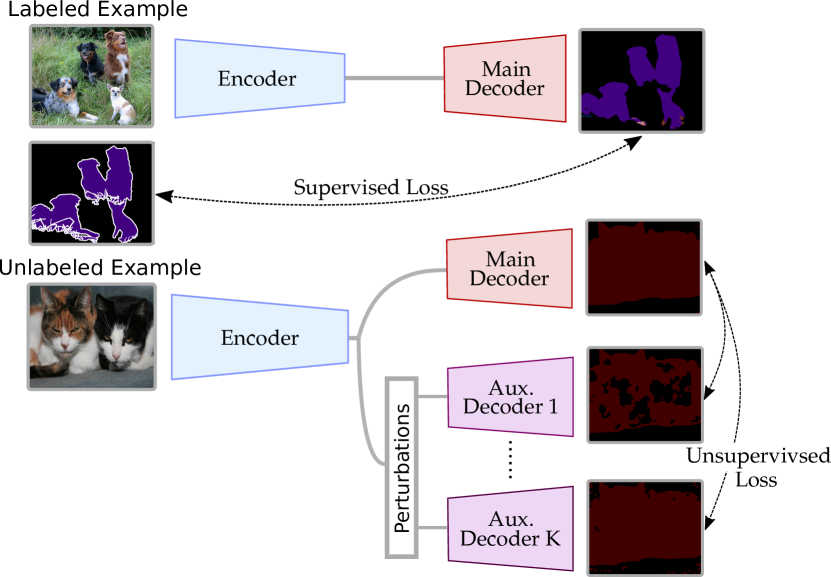
Figure 1: The proposed Cross-Consistency training (CCT). For the labeled examples, the encoder and the main decoder are trained in a supervised manner. For the unlabeled examples, a consistency between the main decoder’s predictions and those of the auxiliary decoders is enforced, over different types of perturbations applied to the inputs of the auxiliary decoders. Best viewed in color.

However, the recent progress in SSL was confined to classification tasks, and its application in semantic segmentation is still limited. Dominant approaches [24, 54, 53, 32] focus on weakly-supervised learning which principle is to generate pseudo pixel-level labels by leveraging the weak labels, that can then be used, together with the limited strongly labeled examples, to train a segmentation network in a supervised manner. Generative Adversarial Networks (GANs) were also adapted for SSL setting [50, 25] by extending the generic GAN framework to pixel-level predictions. The discriminator is then jointly trained with an adversarial loss and a supervised loss over the labeled examples.

Nevertheless, these approaches suffer from some limitations. Weakly-supervised approaches require weakly labeled examples along with pixel-level labels, hence, they do not exploit the unlabeled data to extract additional training signal. Methods based on adversarial training exploit the unlabeled data, but can be harder to train.

To address these limitations, we propose a simple consistency based semi-supervised method for semantic segmentation. The objective in consistency training is to enforce an invariance of the model’s predictions over small perturbations applied to the inputs. As a result, the learned model will be robust to such small changes. The effectiveness of consistency training depends heavily on the behavior of the data distribution, i.e., the cluster assumption, where the classes must be separated by low density regions. In semantic segmentation, we do not observe the presence of low density regions separating the classes within the inputs, but rather within the encoder’s outputs. Based on this observation, we propose to enforce the consistency over different forms of perturbations applied to the encoder’s output. Specifically, we consider a shared encoder and a main decoder that are trained using the labeled examples. To leverage unlabeled data, we then consider multiple auxiliary decoders whose inputs are perturbed versions of the output of the shared encoder. The consistency is imposed between the main decoder’s predictions and that of the auxiliary decoders (see Fig. 1). This way, the shared encoder’s representation is enhanced by using the additional training signal extracted from the unlabeled data. The added auxiliary decoders have a negligible amount of parameters compared to the encoder. Additionally, during inference, only the main decoder is used, reducing the computation overhead both in training and inference.

The proposed method is simple and efficient, it is also flexible since it can easily be extended to use additional weak labels and pixel-level labels across different domains in a semi-supervised domain adaption setting. With extensive experiments, we demonstrate the effectiveness of our approach on PASCAL VOC [14] in a semi-supervised setting, and CityScapes, CamVid [5] and SUN [49] in a semi-supervised domain adaption setting. We obtain competitive results across different datasets and training settings.

Concretely, our contributions are four-fold:

• We propose a cross-consistency training (CCT) method for semi-supervised semantic segmentation, where the invariance of the predictions is enforced over different perturbations injected into the encoder’s output.

• We propose and conduct an exhaustive study of various types of perturbations.

• We extend our approach to use weakly-labeled data, and exploit pixel-level labels across different domains to jointly train the segmentation network.

• We demonstrate the effectiveness of our approach with with an extensive and detailed experimental results, including a comparison with the state-of-the-art, as well as an in-depth analysis of our approach with a detailed ablation study.

2 Related Work

Semi-Supervised Learning. Recently, many efforts have been made to adapt classic SSL methods to deep learning, such as pseudo labeling [31], entropy minimization [19] and graph based methods [35, 27] in order to overcome this weakness. In this work, we focus mainly on consistency training. We refer the reader to [7] for a detailed overview of the field. Consistency training methods are based on the assumption that, if a realistic form of perturbation was applied to the unlabeled examples, the predictions should not change significantly. Favoring models with decision boundaries that reside in low density regions, giving consistent predictions for similar inputs. For example, $\Pi$-Model [30] enforces a consistency over two perturbed versions of the inputs under different data augmentations and dropout. A weighted moving average of either the previous predictions (i.e., Temporal Ensembling [30]), or the model’s parameters (i.e., Mean Teacher [51]), can be used to obtain more stable predictions over the unlabeled examples. Instead of relying on random perturbations, Virtual Adversarial Training (VAT) [37] approximates the perturbations that will alter the model’s predictions the most.

Similarly, the proposed method enforces a consistency of predictions between the main decoder and the auxiliary decoders over different perturbations, that are applied to the encoder’s outputs rather than the inputs. Our work is also loosely related to Multi-View learning [60] and Cross-View training [9], where each input to the auxiliary decoders can be view as an alternate, but corrupt representation of the unlabeled examples.

Semi-Supervised Semantic Segmentation. A significant number of approaches use a limited number pixel-level labels together with a larger number of inexact annotations, e.g., region-level [48, 11] or image-level labels [32, 61, 54, 33]. For image-level based weak-supervision, primary localization maps are generated using class activation mapping (CAM) [61]. After refining the generated maps, they can then be used to train a segmentation network together with the available pixel-level labels in a SSL setting.

Generative modeling can also be used for semi-supervised semantic segmentation [50, 25] to take advantage of the unlabeled examples. Under a GAN framework, the discriminator’s predictions are extended over pixel classes, and can then be jointly trained with a Cross-Entropy loss over the labeled examples and an adversarial loss over the whole dataset.

In comparison, the proposed method exploits the unlabeled examples by enforcing a consistency over multiple perturbations on the hidden representations level. Enhancing the encoder’s representation and the overall performance, with a small additional cost in terms of computation and memory requirements.

Recently, CowMix [15], a concurrent method was introduced. CowMix, using MixUp [57], enforces a consistency between the mixed outputs and the prediction over the mixed inputs. In this context, CCT differs as follows: (1) CowMix, as traditional consistency regularization methods, applies the perturbations to the inputs, but uses MixUp as a high-dimensional perturbation to overcome the absence of the cluster assumption. (2) Requires multiple forward passes though the network for one training iteration. (3) Adapting CowMix to other settings (e.g., over multiple domains, using weak labels) may require significant changes. CCT is efficient and can easily be extended to other settings.

Domain Adaptation. In many real world cases, the existing discrepancy between the distribution of training data and and that of testing data will often hinder the performances. Domain adaptation aims to rectify this mismatch and tune the models for a better generalization at test time [42]. Various generative and discriminative domain adaptation methods have been proposed for classification [18, 16, 17, 6] and semantic segmentation [23, 58, 46, 26] tasks.

In this work, we show that enforcing a consistency across different domains can push the model toward better generalization, even in the extreme case of non-overlapping label spaces.

3 Method

3.1 The cluster assumption in semantic segmentation

We start with our observation and analysis of the cluster assumption in semantic segmentation, motivating the proposal of our cross-consistency training approach. A simple way to examine it is to estimate the local smoothness by measuring the local variations between the value of each pixel and its local neighbors. To this end, we compute the average euclidean distance at each spatial location and its 8 intermediate neighbors, for both the inputs and the hidden representations (i.e., the ResNet’s [22] outputs of a DeepLab v3 [8] trained on COCO [34]). For the inputs, following [15], we compute the average distance of a patch centered at a given spatial location and its neighbors to simulate a realistic receptive field. For the hidden representations, we first upsample the feature map to the input size, and then compute the average distance between the neighboring activations ($2048$-dimensional feature vectors). The results are illustrated in Fig. 7. We observe that the cluster assumption is violated at the input level, given that the low density regions do not align with the class boundaries. On the contrary, for the encoder’s outputs, the cluster assumption is maintained where the class boundaries have high average distance, thus corresponding to low density regions. This observation motivates the following approach, in which the perturbations are applied to the encoder’s outputs rather than the inputs.

3.2 Cross-Consistency Training for semantic segmentation

3.2.1 Problem Definition

In SSL, we are provided with a small set of labeled training examples and a larger set of unlabeled training examples. Let $\mathcal{D}_{l}=\{(\mathbf{x}_{1}^{l},y_{1}),\ldots,(\mathbf{x}_{n}^{l},y_{n})\}$ represent the $n$ labeled examples and $\mathcal{D}_{u}=\{\mathbf{x}_{1}^{u},\ldots,\mathbf{x}_{m}^{u}\}$ represent the $m$ unlabeled examples, with $\mathbf{x}_{i}^{u}$ as the $i$-th unlabeled input image, and $\mathbf{x}_{i}^{l}$ as the $i$-th labeled input image with spatial dimensions $H\times W$ and its corresponding pixel-level label $y_{i}\in\mathbb{R}^{C\times H\times W}$, where $C$ is the number of classes.

As discussed in the introduction, the objective is to exploit the larger number of unlabeled examples ($m\gg n$) to train a segmentation network $f$, to perform well on the test data drawn from the same distribution as the training data. In this work, our architecture (see Fig. 3) is composed of a shared encoder $h$ and a main decoder $g$, which constitute the segmentation network $f=g\circ h$. We also introduce a set of $K$ auxiliary decoders $g_{a}^{k}$, with $k\in[1,K]$. While the segmentation network $f$ is trained on the labeled set $\mathcal{D}_{l}$ in a traditional supervised manner, the auxiliary networks $g_{a}^{k}\circ h$ are trained on the unlabeled set $\mathcal{D}_{u}$ by enforcing a consistency of predictions between the main decoder and the auxiliary decoders. Each auxiliary decoder takes as input a perturbed version of the encoder’s output, and the main encoder is fed the uncorrupted intermediate representation. This way, the representation learning of the encoder $h$ is further enhanced using the unlabeled examples, and subsequently, that of the segmentation network $f$.

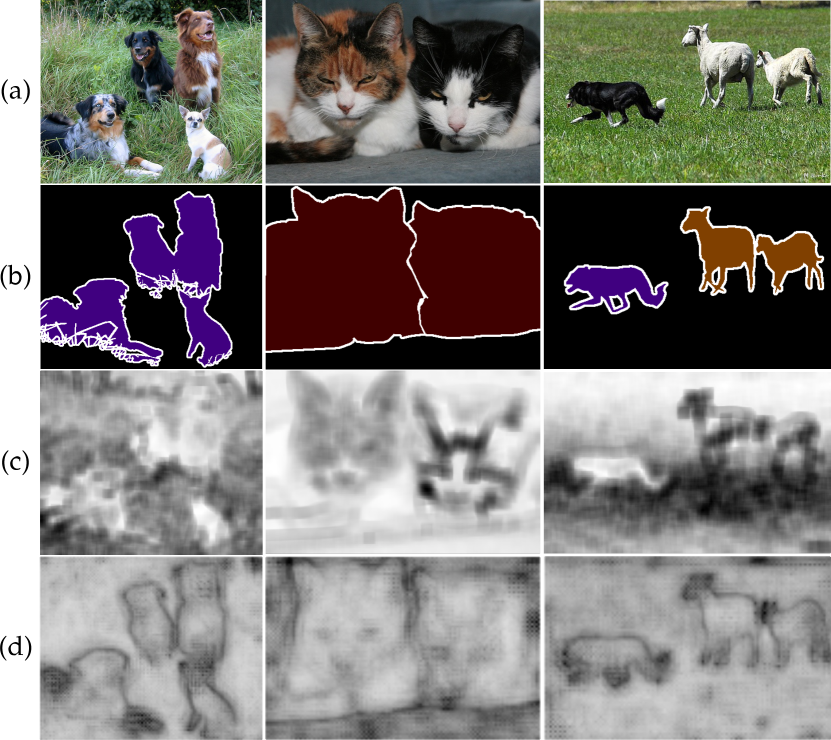
Figure 2: The cluster assumption in semantic segmentation. (a) Examples from PASCAL VOC 2012 train set. (b) Pixel-level labels. (c) Input level. The average euclidean distance between each patch of size $20\times 20$ centered at a given spatial location extracted from the input images, and its 8 neighboring patches. (d) Hidden representations level. The average euclidean distance between a given $2048$-dimensional activation at each spatial location and its 8 neighbors. Darkest regions indicate high average distance.

3.2.2 Cross-Consistency Training

As stated above, to extract additional training signal from the unlabeled set $\mathcal{D}_{u}$, we rely on enforcing a consistency between the outputs of the main decoder $g_{m}$ and those of auxiliary decoders $g_{a}^{k}$. Formally, for a labeled training example $\mathbf{x}_{i}^{l}$, and its pixel-level label $y_{i}$, the segmentation network $f$ is trained using a Cross-Entropy (CE) based supervised loss $\mathcal{L}_{s}$:

$$\mathcal{L}_{s}=\frac{1}{|\mathcal{D}_{l}|}\sum_{\mathbf{x}_{i}^{l},y_{i}\in\mathcal{D}_{l}}\mathbf{H}(y_{i},f(\mathbf{x}_{i}^{l}))$$ (1)

with $\mathbf{H}(.,.)$ as the CE. For an unlabeled example $\mathbf{x}_{i}^{u}$, an intermediate representation of the input is computed using the shared encoder $\mathbf{z}_{i}=h(\mathbf{x}_{i}^{u})$. Let us consider $R$ stochastic perturbations functions, denoted as $p_{r}$ with $r\in[1,R]$, where one perturbation function can be assigned to multiple auxiliary decoders. With various perturbation settings, we generate $K$ perturbed versions $\tilde{\mathbf{z}}_{i}^{k}$ of the intermediate representation $\mathbf{z}_{i}$, so that the $k$-th perturbed version is to be fed to the $k$-th auxiliary decoder. For consistency, we consider the perturbation function as part of the auxiliary decoder, (i.e., $g_{a}^{k}$ can be seen as $g_{a}^{k}\circ p_{r}$). The training objective is then to minimize the unsupervised loss $\mathcal{L}_{u}$, which measures the discrepancy between the main decoder’s output and that of the auxiliary decoders:

$$\mathcal{L}_{u}=\frac{1}{|\mathcal{D}_{u}|}\frac{1}{K}\sum_{\mathbf{x}_{i}^{u}\in\mathcal{D}_{u}}\sum_{k=1}^{K}\mathbf{d}(g(\mathbf{z}_{i}),g_{a}^{k}(\mathbf{z}_{i}))$$ (2)

with $\mathbf{d}(.,.)$ as a distance measure between two output probability distributions (i.e., the outputs of a $softmax$ function applied over the channel dimension). In this work, we choose to use mean squared error (MSE) as a distance measure.

The combined loss $\mathcal{L}$ for consistency based SSL is then computed as:

$$\mathcal{L}=\mathcal{L}_{\text{s}}+\omega_{u}\mathcal{L}_{\text{u}}$$ (3)

where $\omega_{u}$ is an unsupervised loss weighting function. Following [30], to avoid using the initial noisy predictions of the main encoder, $\omega_{u}$ ramps up starting from zero along a Gaussian curve up to a fixed weight $\lambda_{u}$. Concretely, at each training iteration, an equal number of examples are sampled from the labeled $\mathcal{D}_{l}$ and unlabeled $\mathcal{D}_{u}$ sets. The supervised loss is computed using the main encoder’s output and pixel-level labels. For the unlabeled examples, we compute the MSE between the prediction of each auxiliary decoder and that of the main decoder. The total loss is then compute and back-propagated to train the segmentation network $f$ and the auxiliary networks $g_{a}^{k}\circ h$. Note that the unsupervised loss $\mathcal{L}_{u}$ is not back-propagated through the main-decoder $g$, only the labeled examples are used to train $g$.

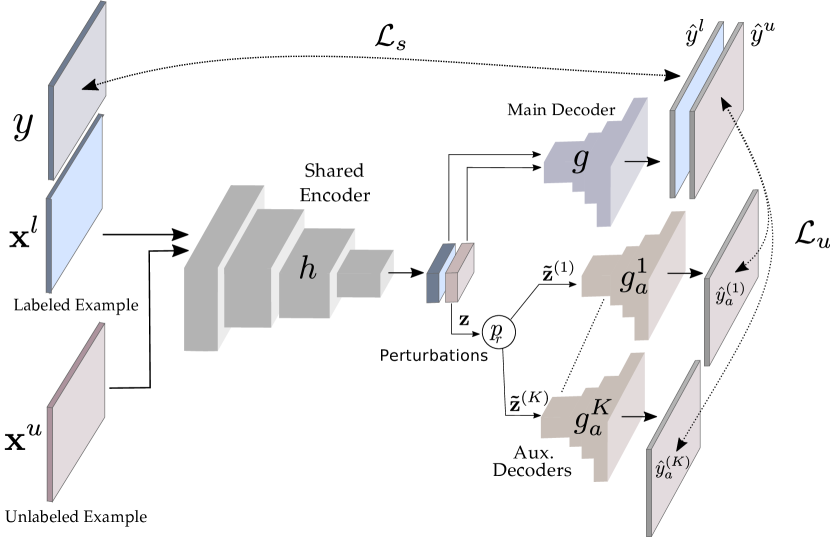
Figure 3: Illustration of our approach. For one training iteration, we sample a labeled input image $\mathbf{x}^{l}$ and its pixel-level label $y$ together with an unlabeled image $\mathbf{x}^{u}$. We pass both images through the encoder and main decoder, obtaining two main predictions $\hat{y}^{l}$ and $\hat{y}^{u}$. We compute the supervised loss using the pixel-level label $y$ and $\hat{y}^{l}$. We apply various perturbations to $\mathbf{z}$, the output of the encoder for $\mathbf{x}^{u}$, and generate auxiliary predictions $\hat{y}^{(i)}_{a}$ using the perturbed versions $\tilde{\mathbf{z}}^{(i)}$. The unsupervised loss is then computed between the outputs of the auxiliary decoders and that of the main decoder.

3.2.3 Perturbation functions

An important factor in consistency training is the perturbations to apply to the hidden representation, i.e., the encoder’s output $\mathbf{z}$. We propose three types of perturbation functions $p_{r}$: feature based, prediction based and random.

Feature based perturbations. They consist of either injecting noise into or dropping some of the activations of encoder’s output feature map $\mathbf{z}$.

• $\operatorname{F-Noise}$: we uniformly sample a noise tensor $\mathbf{N}\sim\mathcal{U}(-0.3,0.3)$ of the same size as $\mathbf{z}$. After adjusting its amplitude by multiplying it with $\mathbf{z}$, the noise is then injected into the encoder’s output $\mathbf{z}$ to get $\tilde{\mathbf{z}}=(\mathbf{z}\odot\mathbf{N})+\mathbf{z}$. This way, the injected noise is proportional to each activation.

• $\operatorname{F-Drop}$: we first uniformly sample a threshold $\gamma\sim\mathcal{U}(0.6,0.9)$. After summing over the channel dimension and normalizing the feature map $\mathbf{z}$ to get $\mathbf{z}^{\prime}$, we generate a mask $\mathbf{M}_{\text{drop}}=\{\mathbf{z}^{\prime}<\gamma\}_{\mathbf{1}}$, which is then used to obtain the perturbed version $\tilde{\mathbf{z}}=\mathbf{z}\odot\mathbf{M}_{\text{drop}}$. This way, we mask $10\%$ to $40\%$ of the most active regions in the feature map.

Prediction based perturbations. They consist of adding perturbations based on the main decoder’s prediction $\hat{y}=g(\mathbf{z})$ or that of the auxiliary decoders. We consider masking based perturbations ($\operatorname{Con-Msk}$, $\operatorname{Obj-Msk}$ and $\operatorname{G-Cutout}$) in addition to adversarial perturbations ($\operatorname{I-VAT}$).

• Guided Masking: Given the importance of context relationships for complex scene understanding [38], the network might be too reliant on these relationships. To limit them, we create two perturbed versions of $\mathbf{z}$ by masking the detected objects ($\operatorname{Obj-Msk}$) and the context ($\operatorname{Con-Msk}$). Using $\hat{y}$, we generate an object mask $\mathbf{M}_{\text{obj}}$ to mask the detected foreground objects and a context mask $\mathbf{M}_{\text{con}}=1-\mathbf{M}_{\text{obj}}$, which are then applied to $\mathbf{z}$.

• Guided Cutout ($\operatorname{G-Cutout}$): in order to reduce the reliance on specific parts of the objects, and inspired by Cutout [13] that randomly masks some parts of the input image, we first find the possible spatial extent (i.e., bounding box) of each detected object using $\hat{y}$. We then zero-out a random crop within each object’s bounding box from the corresponding feature map $\mathbf{z}$.

• Intermediate VAT ($\operatorname{I-VAT}$): to further push the output distribution to be isotropically smooth around each data point, we investigate using VAT [37] as a perturbation function to be applied to $\mathbf{z}$ instead of the unlabeled inputs. For a given auxiliary decoder, we find the adversarial perturbation $r_{adv}$ that will alter its prediction the most. The noise is then injected into $\mathbf{z}$ to obtain the perturbed version $\tilde{\mathbf{z}}=r_{adv}+\mathbf{z}$.

Random perturbations. ($\operatorname{DropOut}$) Spatial dropout [52] is also applied to $\mathbf{z}$ as a random perturbation.

3.2.4 Practical considerations

A each training iteration, we sample an equal number of labeled and unlabeled samples. As a consequence, we iterate on the set $\mathcal{D}_{l}$ more times than on its unlabeled counterpart $\mathcal{D}_{u}$, thus risking an overfitting of the labeled set $\mathcal{D}_{l}$.

Avoiding Overfitting. Motivated by [43] who observed improved results by sampling only $6\%$ of the hardest pixels, and [55] who showed an improvement when gradually releasing the supervised training signal in a SSL setting, we propose an annealed version of the bootstrapped-CE ($\operatorname{ab-CE}$) in [43]. With an output $f(\mathbf{x}_{i}^{l})\in\mathbb{R}^{C\times H\times W}$ in the form of a probability distribution over the pixels, we only compute the supervised loss over the pixels with a probability less than a threshold $\eta$:

$$\mathcal{L}_{s}=\frac{1}{|\mathcal{D}_{l}|}\sum_{\mathbf{x}_{i}^{l},y_{i}\in\mathcal{D}_{l}}\{f(\mathbf{x}_{i}^{l})<\eta\}_{\mathbf{1}}\mathbf{H}(y_{i},f(\mathbf{x}_{i}^{l}))$$ (4)

To release the supervised training signal, the threshold parameter $\eta$ is gradually increased from $\frac{1}{C}$ to $0.9$ during the beginning of training, with $C$ as the number of output classes.

3.3 Exploiting weak-labels

In some cases, we might be provided with additional training data that is less expensive to acquire compared to pixel-level labels, e.g., image-level labels. Formally, instead of an unlabeled set $\mathcal{D}_{u}$, we are provided with a weakly labeled set $\mathcal{D}_{w}=\{(\mathbf{x}_{1}^{w},y_{1}^{w}),\ldots,(\mathbf{x}_{m}^{w},y_{m}^{w})\}$ alongside a pixel-level labeled set $\mathcal{D}_{l}$, with $y_{i}^{w}$ is the $i$-th image-level label corresponding to the $i$-th weakly labeled input image $\mathbf{x}_{i}^{w}$. The objective is to extract additional information from the weak labeled set $\mathcal{D}_{w}$ to further enhance the representations of the encoder $h$. To this end, we add a classification branch $g_{c}$ consisting of a global average pooling layer followed by a classification layer, and pretrain the encoder for a classification task using binary CE loss.

Following previous works [1, 32, 24], the pretrained encoder and the added classification branch can then be exploited to generate pseudo pixel-level labels $y_{p}$. We start by generating the CAMs $M$ as in [61]. Using $M\in\mathbb{R}^{C\times H\times W}$, we can then generate pseudo labels $y_{p}$, with a background $\theta_{bg}$ and a foreground $\theta_{fg}$ thresholds. The pixels with attention scores less than $\theta_{bg}$ (e.g., $0.05$) are considered as background. For the pixels with an attention score larger than $\theta_{fg}$ (e.g., $0.30$), they are assigned the class with the maximal attention score, and the rest of the pixels are ignored. After generating $y_{p}$, we conduct a final refinement step using dense CRF [28].

In addition to considering $\mathcal{D}_{w}$ as an unlabeled set and imposing a consistency over its examples, the pseudo-labels are used to train the auxiliary networks $g_{a}^{k}\circ h$ using a weakly supervised loss $\mathcal{L}_{w}$. In this case, the loss in Eq. 3 becomes:

$$\mathcal{L}=\mathcal{L}_{\text{s}}+\omega_{u}\mathcal{L}_{u}+\omega_{w}\mathcal{L}_{w}$$ (5)

With

$$\mathcal{L}_{w}=\frac{1}{|\mathcal{D}_{w}|}\frac{1}{K}\sum_{\mathbf{x}_{i}^{w}\in\mathcal{D}_{w}}\sum_{k=1}^{K}\mathbf{H}(y_{p},g_{a}^{k}(\mathbf{z}_{i}))$$ (6)

3.4 Cross-Consistency Training on Multiple Domains

In this section, we extend the propose framework to a semi-supervised domain adaption setting. We consider the case of two datasets $\{\mathcal{D}^{(1)},\mathcal{D}^{(2)}\}$ with partially or fully non-overlapping label spaces, each one contains a set of labeled and unlabeled examples $\mathcal{D}^{(i)}=\{\mathcal{D}^{(i)}_{l},\mathcal{D}^{(i)}_{u}\}$. The objective is to simultaneously train a segmentation network to do well on the test data of both datasets, which is drown from the different distributions.

Our assumption is that enforcing a consistency over both unlabeled sets $\mathcal{D}^{(1)}_{u}$ and $\mathcal{D}^{(2)}_{u}$ might impose an invariance of the encoder’s representations across the two domains. To this end, on top of the shared encoder $h$, we add domain specific main decoder $g^{(i)}$ and auxiliary decoders $g_{a}^{k(i)}$. Specifically, as illustrated in Fig. 4, we add two main decoders and $2K$ auxiliary decoders on top of the encoder $h$. During training, we alternate between the two datasets, at each iteration, sampling an equal number of labeled and unlabeled examples from each one, computing the loss in Eq. 3 and training the shared encoder and the corresponding main and auxiliary decoders.

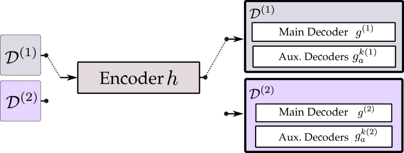
Figure 4: CCT on multiple domains. On top of a shared encoder, we add domain specific main decoder and $K$ auxiliary decoders. During training, we alternate between the two domains, sampling labeled and unlabeled examples and training the corresponding decoders and the shared encoder at each iteration.

4 Experiments

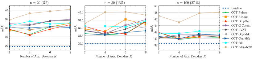
Figure 5: Ablation Studies on CamVid with 20, 50 and 100 labeled images. With different types of perturbations and a variable number of auxiliary decoders $K$, we compare the individual and the combined effectiveness of the perturbations to the baseline in which the model is trained only on the labeled examples. CCT full refers to using all of the 7 perturbations, i.e. the number of auxiliary decoder is $K\times 7$.

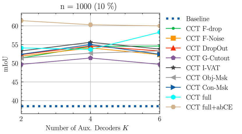
Figure 6: Ablation study on PASCAL VOC. Ablation study results with 1000 labeled examples using different perturbations and various numbers of auxiliary decoders $K$.

To evaluate the proposed method and investigate its effectiveness in different settings, we carry out detailed experiments. In Section 4.4, we present an extensive ablation study to highlight the contribution of each component within the proposed framework, and compare it to state-of-the-art methods in a semi-supervised setting. Additionally, in Section 4.5 we apply the proposed method in a semi-supervised domain adaptation setting and show performance above baseline methods.

4.1 Network Architecture

Encoder. For the following experiments, the encoder is based on a ResNet-50 [22] pretrained on ImageNet [12] provided by [56] and a PSP module [59]. Following previous works [59, 24, 1], the last two strided convolutions of ResNet are replaced with dilated convolutions.

Decoders. For the decoders, taking the efficiency and the number of parameters into consideration, we choose to only use $1\times 1$ convolutions. After an initial $1\times 1$ convolution to adapt the depth to the number of classes $C$, we apply a series of three sub-pixel convolutions [47] with ReLU non-linearities to upsample the outputs to original input size.

4.2 Datasets and Evaluation Metrics

Datasets. In a semi-supervised setting, we evaluate the proposed method on PASCAL VOC [14], consisting of 21 classes (with the background included) and three splits, training, validation and testing, with of $1464$, $1449$ and $1456$ images respectively. Following the common practice [24, 59], we augment the training set with additional images from [21]. Note that the pixel-level labels are only extracted from the original training set.

For semi-supervised domain adaption, for partially overlapping label spaces, we train on both Cityscapes [10] and CamVid [5]. Cityscapes is a finely annotated autonomous driving dataset with $19$ classes. We are provided with three splits, training, validation and testing with $2975$, $500$ and $1525$ images respectively. CamVid contains 367 training, 101 validation and 233 testing images. Although originally the dataset is labeled with $38$ classes, we use the $11$ classes version [2]. For experiments over non-overlapping labels spaces, we train on Cityscapes and SUN RGB-D [49]. SUN RGB-D is an indoor segmentation dataset with $38$ classes containing two splits, training and validation, with $5285$ and $5050$ images respectively. Similar to [26], we train on the $13$ classes version [20].

Evaluation Metrics. We report the results using mIoU (i.e., mean of class-wise intersection over union) for all the datasets.

4.3 Implementation Details

Training Settings. The implementation is based on the PyTorch 1.1 [41] framework. For optimization, we train for $50$ epochs using SGD with a learning rate of $0.01$ and a momentum of $0.9$. During training, the learning rate is annealed following the poly learning rate policy, where at each iteration, the base learning rate is multiplied by $1-(\frac{\operatorname{iter}}{\operatorname{max\_iter}})^{\operatorname{power}}$ with $\operatorname{power}=0.9$.

For PASCAL VOC, we take crops of size $321\times 321$ and apply random rescaling in the range of $[0.5,2.0]$ and random horizontal flip. For Cityscapes, Cam-Vid and SUN RGB-D, following [26, 25], we resize the input images to $512\times 1024$, $360\times 480$ and $480\times 640$ respectively, without any data-augmentation.

Reproducibility All the experiments are conducted on a V-100 GPUs. The implementation is available at: https://github.com/yassouali/CCT

Inference Settings. For PASCAL VOC, Cityscapes and SUN RGB-D, we report the results obtained on the validation set, and on the test set of CamVid dataset.

4.4 Semi-Supervised Setting

4.4.1 Ablation Studies

The proposed method consists of several types of perturbations and a variable number of auxiliary decoders. We thus start by studying the effect of the perturbation functions with different numbers of auxiliary decoders, in order to provide additional insight into their individual performance and their combined effectiveness. Specifically, we measure the effect of different numbers of auxiliary decoders $K$ (i.e., $K=2$, $4$, $6$ and $8$) of a given perturbation type. We refer to this setting of our method as “CCT {perturbation type}”, with seven possible perturbations. We also measure the combined effect of all perturbations resulting in $K\times 7$ auxiliary decoders in total, and refer to it as “CCT full”. Additionally, “CCT full+$\operatorname{ab-CE}$” indicates the usage of the annealed-bootstrapped CE as a supervised loss function. We compare them to the baseline, in which the model is trained only using the labeled examples.

Method	Pixel-level Labeled Examples	Image-level Labeled Examples	Val
WSSL [40]	1.5k	9k	64.6
GAIN [33]	1.5k	9k	60.5
MDC [54]	1.5k	9k	65.7
DSRG [24]	1.5k	9k	64.3
Souly et al. [50]	1.5k	9k	65.8
FickleNet [32]	1.5k	9k	65.8
Souly et al. [50]	1.5k	-	64.1
Hung et al. [25]	1.5k	-	68.4
CCT	1k	-	64.0
CCT	1.5k	-	69.4
CCT	1.5k	9k	73.2

Table 1: Comparison with the-state-of-the-art. CCT performance on PASCAL VOC compared to other semi-supervised approaches.

CamVid. We carried out the ablation on CamVid with 20, 50 and 100 labels; the results are shown in Fig. 5. We find that each perturbation outperforms the baseline, with the most dramatic differences in the 20-label setting with up to $21$ points. We also surprisingly observe an insignificant overall performance gap among different perturbations, confirming the effectiveness of enforcing the consistency over the hidden representations for semantic segmentation, and highlighting the versatility of CCT and its success with numerous perturbations. Increasing $K$ results in a modest improvement overall, with the smallest change for $\operatorname{Con-Msk}$ and $\operatorname{Obj-Msk}$ due to their lack of stochasticity. Interestingly, we also observe a slight improvement when combining all of the perturbations, indicating that the encoder is able to generate representations that are consistent over many perturbations, and subsequently, improving the overall performance. Additionally, gradually releasing the training signal using $\operatorname{ab-CE}$ helps increase the performance with up to $8\%$, which confirms that overfitting of the labeled examples can cause a significant drop in performance.

PASCAL VOC. In order to investigate the success of CCT on larger datasets, we conduct additional ablation experiments on PASCAL VOC using 1000 labeled examples, The results are summarized in Fig. 6. We see similar results, where the proposed method makes further improvement compared to the baseline with different perturbations, from $10$ to $15$ points. The combined perturbations yield a small increase in the performance, with the biggest difference with $K=6$. Furthermore, similar to CamVid, when using the $\operatorname{ab-CE}$ loss, we see a significant gain with up to $7$ points compared to CCT full.

Based on the conducted ablation studies, for the rest of the experiments, we use the setting of “CCT full” with $K=2$ for $\operatorname{Con-Msk}$ and $\operatorname{Obj-Msk}$ due to their lack of stochasticity, $K=2$ for $\operatorname{I-VAT}$ given its high computational cost, and $K=6$ for the rest of the perturbations, and refer to it as “CCT”.

4.4.2 Comparison to Previous Work

To further explore the effectiveness of our framework, we quantitatively compare it with previous semi-supervised semantic segmentation methods on PASCAL VOC. Table 1 compares CCT with other semi-supervised approaches. Our approach outperforms previous works relying on the same level of supervision and even methods which exploit image-level labels. We also observe an increase of $3.8$ points when using additional image-level labels, affirming the flexibility of CCT, and the possibility of using it with different types of labels without any learning conflicts.

4.5 Semi-Supervised Domain Adaptation Setting

In real world applications, we are often provided with pixel-level labels collected from various sources, thus distinct data distributions. To examine the effectiveness of CCT when applied to multiple domains with a variable degree of labels overlap, we train our model simultaneously on two datasets, Cityscapes (CS) + CamVid (CVD) for partially overlapping labels, and Cityscapes + SUN RGB-D (SUN) for the disjoint case.

Method	n=50				n=100
	CS	CVD	Avg.		CS	CVD	Avg.
Kalluri, et al. [26]	34.0	53.2	43.6		41.0	54.6	47.8
Baseline	31.2	40.0	35.6		37.3	34.4	35.9
CCT	35.0	53.7	44.4		40.1	55.7	47.9

Table 2: CCT applied to CS+CVD. CCT performance when simultaneously trained on two datasets with overlapping label spaces, which are Cityscapes (CS) and CamVid (CVD).

Cityscapes + CamVid. The results for CCT on Cityscapes and CamVid datasets with 50 and 100 labeled examples are given in Table 7. Similar to the SSL setting, CCT outperforms the baseline significantly, where the model is iteratively trained using only on the labeled examples, with up to 12 points for $n=100$, we even see a modest increase compared to previous work. This confirms our hypothesis that enforcing a consistency over different datasets does indeed push the encoder to produce invariant representation across different domains, and consequently, increases the performance over the baseline while delivering similar results on each domain individually.

Method	Labeled Examples		CS	SUN	Avg.
SceneNet [36]	Full (5.3k)		-	49.8	-
Kalluri, et al. [26]	1.5k		58.0	31.5	44.8
Baseline	1.5k		54.3	38.1	46.2
CCT	1.5k		58.8	45.5	52.1

Table 3: CCT applied to CS+CVD. CCT performance when trained on both datasets Cityscapes (CS) and SUN RGB-D (SUN) datasets, for the case of non-overlapping label spaces.

Cityscapes + SUN RGB-D. For cross domain experiments, where the two domains have distinct labels spaces, we train on both Cityscapes and SUN RGB-D to demonstrate the capability of CCT to extract useful visual relationships and perform knowledge transfer between dissimilar domains, even in completely different settings. The results are shown in Table 7. Interestingly, despite the distribution mismatch between the datasets, and the high number of labeled examples ($n=1500$), CCT still provides a meaningful boost over the baseline with 5.9 points difference and 7.3 points compared to previous work. Showing that, by enforcing a consistency of predictions on the unlabeled sets of the two datasets over different perturbations, we can extract additional training signal and enhance the representation learning of the encoder, even in the extreme case with non-overlapping label spaces, without any performance drop when an invariance of representations across both datasets is enforced at the level of encoder’s outputs.

5 Conclusion

In this work, we present cross-consistency training (CCT), a simple, efficient and flexible method for a consistency based semi-supervised semantic segmentation, yielding state-of-the-art results. For future works, a possible direction is exploring the usage of other perturbations to be applied at different levels within the segmentation network. It would also be interesting to adapt and examine the effectiveness of CCT in other visual tasks and learning settings, such as unsupervised domain adaptation.

Acknowledgements. This work was supported by Randstad corporate research chair. We would also like to thank Saclay-IA plateform of Université Paris-Saclay and Mésocentre computing center of CentraleSupélec and École Normale Supérieure Paris-Saclay for providing the computational resources.

Supplementary Material

A Comparison with Traditional Consistency Training Methods

In this section, we present the experiments to validate the observation that for semantic segmentation, enforcing a consistency over different perturbations applied to the encoder’s outputs rather than the inputs is more aligned with the cluster assumption. To this end, we compare the proposed method with traditional consistency based SSL methods. Specifically, we conduct experiments using VAT [37] and Mean Teachers [51]. In VAT, at each training iteration, the unsupervised loss is computed as the KL-divergence between the model’s predictions of the input $\mathbf{x}^{u}$ and its perturbed version $\mathbf{x}^{u}+r_{adv}$. For Mean Teachers, the discrepancy is measured using Mean Squared Error (MSE) between the prediction of the model and the prediction using an exponential weighted version of it. In this case, the noise is sampled at each training step with SGD.

Splits	n=500	n=1000
Baseline	51.4	59.2
Mean Teachers	51.3	59.4
VAT	50.0	57.9
CCT	58.6	64.4

Table 4: CCT compared to traditional consistency methods. We conduct an ablation study on PASCAL VOC, where we compare the performance of the baseline to the proposed method CCT, VAT and Mean Teachers. $n$ represents the number of labeled examples.

The results are presented in Table 4. We see that applying the adversarial noise to inputs with VAT results in lower performance compared to the baseline. When using Mean Teachers, in which the noise is not implicitly added to the inputs, we obtain similar performance to the baseline. These results confirm our observation that enforcing a consistency over perturbations applied to the hidden representations is more aligned with the cluster assumption, thus yielding better results.

B Additional Results and Evaluations

B.1 Distance Measures

In the experiments presented in Section 4.4, MSE was used as a distance measure $\mathbf{d}(.,.)$ for the unsupervised loss $\mathcal{L}_{u}$, to measure the discrepancy between the main and auxiliary predictions. In this section, we investigate the effectiveness of other distance measures between the output probability distributions. Specifically, we compare the performance of MSE to the KL-divergence and the JS-divergence. For an unlabeled example $\mathbf{x}^{u}$, we obtain a main prediction $y^{u}$ with the main decoder and an auxiliary prediction $y_{a}^{k}$ with a given auxiliary decoder $g_{a}^{k}$. We compare the following distance measures:

$$\mathbf{d}_{\text{MSE}}(y^{u},y_{a}^{k})=\frac{1}{N}\sum_{i}^{N}(y^{u}(i)-y_{a}^{k}(i))^{2}$$ (7)

$$\mathbf{d}_{\text{KL}}(y^{u},y_{a}^{k})=\frac{1}{N}\sum_{i}^{N}y^{u}(i)\log\frac{y^{u}(i)}{y_{a}^{k}(i)}$$ (8)

$$\mathbf{d}_{\text{JS}}(y^{u},y_{a}^{k})=\frac{1}{2}\mathbf{d}_{\text{KL}}(y^{u},m)+\frac{1}{2}\mathbf{d}_{\text{KL}}(y_{a}^{k},m)$$ (9)

where $m=\frac{1}{2}(y^{u}(i)+y_{a}^{k}(i))$ and $y^{*}(i)$ refers to the output probability distribution at a given spatial location $i$. The results of the comparison are shown in Table 5.

Splits	n=500	n=1000
Baseline	51.4	59.2
CCT KL	54.0	62.5
CCT JS	58.4	64.3
CCT MSE	58.6	64.4

Table 5: CCT with different distance measures. We compare the performance of MSE to the KL-divergence and the JS-divergence on PASCAL VOC dataset.

We observe similar performance with $\mathbf{d}_{\text{MSE}}$ and $\mathbf{d}_{\text{JS}}$, while we only obtain 2.6 and 3.3 points gain for $n=500$ and $n=1000$ respectively over the baseline when using $\mathbf{d}_{\text{KL}}$. The low performance of $\mathbf{d}_{\text{KL}}$ might be due to its non-symmetric nature. With $\mathbf{d}_{\text{KL}}$, the auxiliary decoders are heavily penalized over sharp but wrong predictions, thus pushing them to produce uniform and uncertain outputs, and reducing the amount of training signal that can be extracted from the unlabeled examples. However, with $\mathbf{d}_{\text{JS}}$, which is a symmetrized and smoothed version of $\mathbf{d}_{\text{KL}}$, we can bypass the zero avoidance nature of the KL-divergence. Similarly, $\mathbf{d}_{\text{MSE}}$ can be seen as a multi-class Brier score [4] which is less sensitive to completely incorrect predictions, giving it similar properties to $\mathbf{d}_{\text{JS}}$ with a lower computational cost.

B.2 Confidence Masking and Pairwise Loss

Confidence Masking. ($\operatorname{Conf-Mask}$)

When training on the unlabeled examples, we use the main predictions as the source for consistency training, which may result in a corrupted training signal when based on uncertain predictions. A possible way to avoid this is masking the uncertain predictions. Given a main prediction $y^{u}$ in the form of a probability distribution over the classes $C$ at different spatial locations $i$. We compute the unsupervised loss $\mathcal{L}_{u}$ only over the pixels $i$ with probability $\max\limits_{C}y^{u}(i)$ greater than a fixed threshold $\beta$ (e.g., 0.5).

Pairwise Loss. ($\operatorname{P-Wise}$)

In CCT, we enforce the consistency of predictions only between the main and auxiliary decoders, without any pairwise consistency in between the auxiliary predictions. To investigate the effectiveness of enforcing such an additional pairwise consistency, we add the following an additional loss term $\mathcal{L}_{\operatorname{P-Wise}}$ to the total loss in Eq. 3 to penalize the auxiliary predictive variance:

$$\mathcal{L}_{\operatorname{P-Wise}}=\frac{1}{K}\sum_{k=1}^{K}(y_{a}^{k}-\bar{y}_{a})^{2}$$ (10)

with $\bar{y}_{a}$ as the mean of the auxiliary predictions $y_{a}^{k}$. Given $K$ auxiliary decoders, the computation of $\mathcal{L}_{\operatorname{P-Wise}}$ is in the order of $K^{2}$. To reduce it, at each training iteration, we only compute $\mathcal{L}_{\operatorname{P-Wise}}$ over a randomly chosen subset of the auxiliary predictions (e.g., $8$ out of $K=30$).

Table 6 shows the results of the experiments when using CCT with $\operatorname{Conf-Mask}$ and $\operatorname{P-Wise}$. Interestingly, we do not observe any gain over CCT when using $\operatorname{Conf-Mask}$, indicating that using the uncertain main predictions to enforce the consistency does not hinder the performance. Additionally, adding a pairwise loss term results in lower performance compared to CCT, with $3$ and $3.2$ points difference in both settings, indicating that adding $\mathcal{L}_{\operatorname{P-Wise}}$ can potentially compel the auxiliary decoders to produce similar predictions regardless of the applied perturbation, thus diminishing the representation learning of the encoder, and the performance of the segmentation network as a whole.

Splits	n=500	n=1000
Baseline	51.4	59.2
CCT +$\operatorname{Conf-Mask}$	58.4	63.3
CCT +$\mathcal{L}_{\operatorname{P-Wise}}$	55.6	61.2
CCT	58.6	64.4

Table 6: CCT with $\operatorname{P-Wise}$ and $\operatorname{Conf-Mask}$. The results of the effect of adding a confidence masking over unsupervised loss and a pairwise loss between the auxiliary predictions on PASCAL VOC val set.

C Algorithm

The proposed Cross-Consistency training method can be summarized by the following Algorithm:

Input: Labeled image $\mathbf{x}^{l}$, its pixel-level label $y$ and unlabeled image $\mathbf{x}^{u}$

Require: Shared encoder $h$, main decoder $g_{m}$, $K$ auxiliary decoders $g_{a}^{k}$

1) Forward $\mathbf{x}^{l}$ through the encoder and main decoder: $\hat{y}^{l}=g_{m}(h(\mathbf{x}^{l}))$

2) Forward the unlabeled input through the shared encoder: $\mathbf{z}=h(\mathbf{x}^{u})$

3) Generate the main decoder’s prediction for $\mathbf{x}^{u}$: $\hat{y}^{u}=g_{m}(\mathbf{z})$

4) Generate the aux. decoders predictions for $\mathbf{x}^{u}$:

for $k$ in $[1,K]$ do

      - Apply a given perturbation $\tilde{\mathbf{z}}=p_{l}(z)$

      - Forward through the aux. decoder $k$: $\hat{y}_{a}^{i}=g_{a}^{k}(\tilde{\mathbf{z}})$

     

      end for

     5) Training the network.

      $\mathcal{L}_{s}=\mathbf{H}(\hat{y}^{u},y)$

      $\mathcal{L}_{u}=\frac{1}{K}\sum_{k}\mathbf{d}(\hat{y}^{u},\hat{y}_{a}^{k})$

Update network by $\mathcal{L}=\mathcal{L}_{s}+\omega_{u}\mathcal{L}_{u}$

Algorithm 1 Cross-Consistency Training (CCT).

D Further Investigation of The Cluster Assumption

The learned feature of a CNNs are generally more homogeneous, and at higher layers, the network learns to compose low level features into semantically meaningful representations while discarding high-frequency information (e.g., texture). However, the leaned features in a segmentation network seem to have a unique property; the class boundaries correspond to low density regions, which are not observed in networks trained on other visual tasks (e.g., classification, object detection). See Fig. 7 for an illustration of this difference.

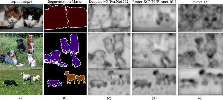
Figure 7: The smoothness of CNNs features trained on different tasks. (a) Examples from PASCAL VOC 2012 train set. (b) Results for a segmentation network. (c) Results for an object detection network. (b) Results for a classification network.

E Adversarial Distribution Alignment

When applying CCT over multiple domains, and to further reduce the discrepancy between the encoder’s representations of the two domains (i.e., the empirical distribution mismatch measured by the $\mathcal{H}$-Divergence [3]), we investigate the addition of a discriminator branch $g_{d}$, which takes as input the encoder’s representation $\mathbf{z}$, and predict 0 for examples from $\mathcal{D}^{(1)}$ and 1 for examples from $\mathcal{D}^{(2)}$. Hence, we add the following adversarial loss to the total loss in Eq. 1:

$$\mathcal{L}_{adv}=\frac{1}{|\mathcal{D}^{(1)}|}\sum_{\mathbf{x}_{i}\in\mathcal{D}^{(1)}}\log(g_{d}(\mathbf{z}_{i}))+\frac{1}{|\mathcal{D}^{(2)}|}\sum_{\mathbf{x}_{i}\in\mathcal{D}^{(2)}}(1-\log(g_{d}(\mathbf{z}_{i})))$$ (11)

The encoder and the discriminator branch are competitors within a min-max framework, i.e., the training objective is $\displaystyle\max_{g_{d}}\min_{h}\mathcal{L}_{adv}$, which can be directly optimized using a gradient reversal layer as in [16]. The total loss in this case is:

$$\mathcal{L}=\mathcal{L}_{s}+\lambda_{adv}\mathcal{L}_{adv}+\omega_{u}\mathcal{L}_{u}$$ (12)

Method	n=50				n=100
	CS	CVD	Avg.		CS	CVD	Avg.
Baseline	31.2	40.0	35.6		37.3	34.4	35.9
CCT	35.0	53.7	44.4		40.1	55.7	47.9
CCT +$\mathcal{L}_{avd}$	35.3	49.2	42.2		37.7	52.8	45.2

Table 7: CCT applied to CS+CVD.

For the discriminator branch, similar to [25], we use a fully convolutional discriminator, with a series of $3\times 3$ convolutions and Leaky ReLU non-linearities as shown in Table 8. The outputs are of the same size as the encoder outputs (i.e. with an input image of spatial dimensions $H\times W$, the outputs of $g_{d}$ are of size $2\times\frac{H}{8}\times\frac{W}{8}$).

Description	Resolution $\times$ channels
Conv $3\times 3\times 64$	$\tfrac{1}{8}\times 64$
LeakyReLU
Conv $3\times 3\times 128$	$\tfrac{1}{8}\times 128$
LeakyReLU
Conv $3\times 3\times 256$	$\tfrac{1}{8}\times 256$
LeakyReLU
Conv $3\times 3\times 512$	$\tfrac{1}{8}\times 512$
LeakyReLU
Conv $1\times 1\times 2$	$\tfrac{1}{8}\times 2$

Table 8: Discriminator Branch. The added discriminator branch on top of the encoder, in order to further push towards an invariance of the encoder’s representations between the different domains.

The results are shown in Table 8. Surprisingly, adding a discriminator branch diminishes the performance of the segmentation network, hinting to possible learning conflicts between CCT and the adversarial loss.

F Multi-scale Inference

To further enhance the predictions of our segmentation network, we conduct additional evaluations on PASCAL VOC using multi-scale to simulate a similar situation to training where we apply random scaling between $0.5$ and $2$, random croping and random horizontal flip. We apply the same augmentations during test. For a given test image, we create 5 versions using 5 scales: $0.5$, $0.75$, $1$, $1.25$ and $1.5$, each image is also flipped horizontally, resulting in $10$ versions of the test image. The model’s prediction are computed for each image, rescaled to the original size, and are then aggregated by pixel-wise average pooling. The final result is obtain by taking the $argmax$ over the classes for each spatial location.

In Table 9, we report the results obtained with multi-scale inference.

	n	mIoU
CCT	1000	67.3 (+3.3)
CCT	1500	73.4 (+4)
CCT +$9k$ Image-level labels	1500	75.1 (+2.9)

Table 9: CCT results with multi-scale inference. The mIoU when we apply multi-scale inference on PASCAL VOC val set.

G Virtual Adversarial Training (VAT)

Without the label information in a semi-supervised setting, VAT [37] lends itself as a consistency regularization technique. It trains the output distribution to be isotropically smooth around each data point by selectively smoothing the model in its most anisotropic direction. In our case, we apply the adversarial perturbation $r_{adv}$ to the encoder output $\mathbf{z}=h(\mathbf{x}^{u})$. For a given auxiliary decoder $g_{a}^{k}$, we would like to compute the adversarial perturbation $r_{adv}$ that will alter its predictions the most. We start by sampling a Gaussian noise $r$ of the same size as $\mathbf{z}$, compute its gradients $grad_{r}$ with respect the loss between the two predictions, with and without the injections of the noise $r$ (i.e., KL-divergence is used as a distance measure $\mathbf{d}(.,.)$). $r_{adv}$ can then be obtained by normalizing and scaling $grad_{r}$ by a hyperparameter $\epsilon$. This can be written as follows:

$$r\sim\mathcal{N}\left(0,\frac{\xi}{\sqrt{dim(\mathbf{z})}}I\right)$$ (13)

$$grad_{r}=\nabla_{r}\mathbf{d}\left(g_{a}^{k}(\mathbf{z}),g_{a}^{k}(\mathbf{z}+r)\right)$$ (14)

$$r_{adv}=\epsilon\frac{grad_{r}}{\|grad_{r}\|}$$ (15)

Finally, the perturbed input to $g_{a}^{k}$ is $\tilde{\mathbf{z}}=r_{adv}+\mathbf{z}$. The main drawback of such method is requiring multiple forward and backward passes for each training iteration to compute $r_{adv}$. In our case, the amount of computations needed are reduced given the small size of the auxiliary decoders.

H Dataset sizes

For the size of each split of the datasets used in our experiments, see Table 10.

Splits	Train	Val	Test
PASCAL VOC	10582	1449	1456
Cityscapes	2975	500	1525
CamVid	367	101	233
SUN RGB-D	5285	-	5050

Table 10: Semantic Segmentation Datasets. The size of each split of the datasets used in the experiments.

I Further Experimental Details

For the experiments throughout the paper, we used a ResNet 50 and a PSP module [59] for the encoder. As for the decoders, we used an initial $1\times 1$ convolutions to adapt the depth to the number of classes $C$, followed by a series of $1\times 1$ sub-pixel convolutions [47] (i.e., PixelShuffle) to upsample the feature maps to the original size. For details see Table 11.

Encoder		Decoder
Description	Resolution $\times$ channels	Description	Resolution $\times$ channels
ResNet 50	$\tfrac{1}{8}\times 2048$	Conv $1\times 1\times C$	$\tfrac{1}{8}\times C$
PSPModule [59]	$\tfrac{1}{8}\times 512$	Conv $1\times 1\times 4C$	$\tfrac{1}{8}\times 4C$
		PixelShuffle	$\tfrac{1}{4}\times C$
		Conv $1\times 1\times 4C$	$\tfrac{1}{4}\times 4C$
		PixelShuffle	$\tfrac{1}{2}\times C$
		Conv $1\times 1\times 4C$	$\tfrac{1}{2}\times 4C$
		PixelShuffle	$1\times C$

Table 11: Encoder-Decoder architecture. Showing the layer type, the number of the outputs channels and the spatial resolution.

Inference Settings. For PASCAL VOC, during the ablation studies reported in Fig. 6, in order to reduce the training time, we trained on smaller size image. Specifically, we resize the bigger side to $300$ and randomly take crops of size $240\times 240$. For the comparisons with state-of-the-art we resize the bigger side to $400$ and take crops of size $321\times 321$ and conduct the inference on the original sized images. For the rest of the datasets, the evaluation is conducted on the same sizes as the ones used during training.

J Hyperparameters

In order to present a realistic evaluation of the proposed method, and following the practical considerations mentioned in [39]. We avoid any form of intensive hyperparameter search, be it that of the perturbation functions, model architecture or training settings. We choose the hyperparameters that resulted in stable training by hand, we do expect however that better performances can be achieved with a comprehensive search. The hyperparameters settings used in the experiments are summarized in Table 12.

Training
SGD
Learning rate	$10^{-2}$
Momentum	$0.9$
Weight Decay	$10^{-4}$
Number of training epochs
PASCAL VOC	50
CamVid	50
Cityscapes & CamVid	50
Cityscapes & SUN RGB-D	100
Losses
Unsupervised loss $\mathcal{L}_{u}$
Rampup periode for $\mathcal{L}_{u}$	0.1
$\mathcal{L}_{u}$ weight $\lambda_{u}$	30
Weakly-supervised loss $\mathcal{L}_{w}$
Rampup periode for $\mathcal{L}_{w}$	0.1
$\mathcal{L}_{w}$ weight $\lambda_{w}$	0.4
Annealed Cross-Entropy loss $\operatorname{ab-CE}$
Rampup periode	0.5
Final threshold	0.9
Adversarial loss $\mathcal{L}_{adv}$
Weight $\lambda_{adv}$	$2.10^{-2}$
Perturbation Functions
$\operatorname{I-VAT}$
VAT $\epsilon$	2.0
VAT $\xi$	$10^{-6}$
$\operatorname{DropOut}$
Dropout rate $p$	$0.5$
$\operatorname{G-Cutout}$
Area of the dropped region	0.4
$\operatorname{F-Drop}$
Drop threshold range	$[0.6,0.9]$
$\operatorname{F-Noise}$
The uniform noise range	$[-0.3,0.3]$

Table 12: Hyperparameters. The hyperparameter settings used in our experiments.

K Ramp-up functions

For the unsupervised loss in Eq. 2, the weighting function $w_{u}$ is gradually increased from $0$ up to a fixed final weight $\lambda_{u}$. The rate of increase can follow many possible rates depending on the schedule used. Fig. 8 shows different ramp-up schedules. For our experiments, following [30], $w_{u}$ ramps-up following an exp-schedule:

$$w_{u}(t)=\min(\lambda_{u},e^{5(\frac{t}{T}-1)}\times\lambda_{u})$$ (16)

with $t$ as the current training iteration and $T$ as the desired ramp-up length (e.g., the first $10\%$ of training time). Similarly, the threshold $\eta$ in the $\operatorname{ab-CE}$ loss (Eq. 4) is gradually increased starting from $1/C$, with $C$ as the number of classes, up to a final threshold $\alpha$ (e.g., $0.9$) within a ramp-up period $T$ (e.g., the first $40\%$ of training time). For $\operatorname{ab-CE}$, we use a log-schedule to quickly increase $\eta$ in the beginning of training:

$$\eta(t)=\min(\alpha,(1-e^{-5\frac{t}{T}})\times(\alpha-1/C)+1/C)$$ (17)

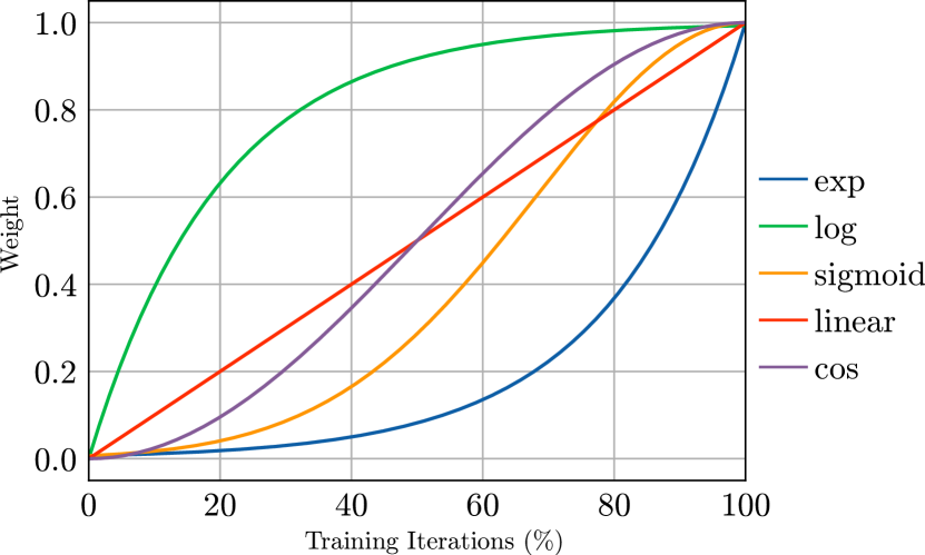
Figure 8: Different ramp-up schedules.

L Computational Overhead

Decoders	Input size	GPU memory (MB)	GPU time (ms)
Main Decoder	$96\times 96$	139	2.0
$\operatorname{DropOut}$		139	2.6
$\operatorname{F-Drop}$		157	3.0
$\operatorname{F-Noise}$		175	45.7
$\operatorname{I-VAT}$		463	82.3
$\operatorname{Obj-Msk}$		463	2.7
$\operatorname{Con-Msk}$		463	2.4
$\operatorname{G-Cutout}$		463	3.3
Main Decoder	$256\times 128$	457	4.0
$\operatorname{DropOut}$		520	4.7
$\operatorname{F-Drop}$		520	5.2
$\operatorname{F-Noise}$		584	149.5
$\operatorname{I-VAT}$		1592	176.0
$\operatorname{Obj-Msk}$		1592	4.7
$\operatorname{Con-Msk}$		1592	4.6
$\operatorname{G-Cutout}$		1592	7.1

Table 13: Computation and memory statistics. Comparisons between the main and auxiliary decoders with different perturbation functions. The channel numbers of the input feature maps $\mathbf{z}$ is $512$. The lower the values, the better.

In order to present a comparison between the computational overhead of the different types of auxiliary decoders, we present various computation and memory statistics in Table 13. We observe that for the majority of the auxiliary decoders, the GPU time is similar to that of the main decoder. However, we see a significant increase for $\operatorname{I-VAT}$ given the multiple forward and backward passes required to compute the adversarial perturbation. $\operatorname{F-Noise}$ also results in high GPU time due to the sampling procedure. To this end we reduce the number of $\operatorname{I-VAT}$ decoders (e.g., $K=2$ for our experiments). For $\operatorname{F-Noise}$, for an input tensor of size $B\times C\times H\times W$ with $B$ as the batch size, instead of sampling a noise tensor $\mathbf{N}$ of the same size, we sample a tensor of size $1\times C\times H\times W$ and apply it over the whole batch. Significantly reduces the computation the computation time without impacting the performance.

M Change Log

v1 Initial Release. Paper accepted to CVPR 2020, the implementation will soon be made available.

N Qualitative Results

Pseudo-Labels

Fig. 9 shows some qualitative results of the generated pseudo pixel-level labels using the available image-level labels. We observe that when considering regions with high attention scores (i.e. $>0.3$), the assigned classes do correspond in most cases to true positives.

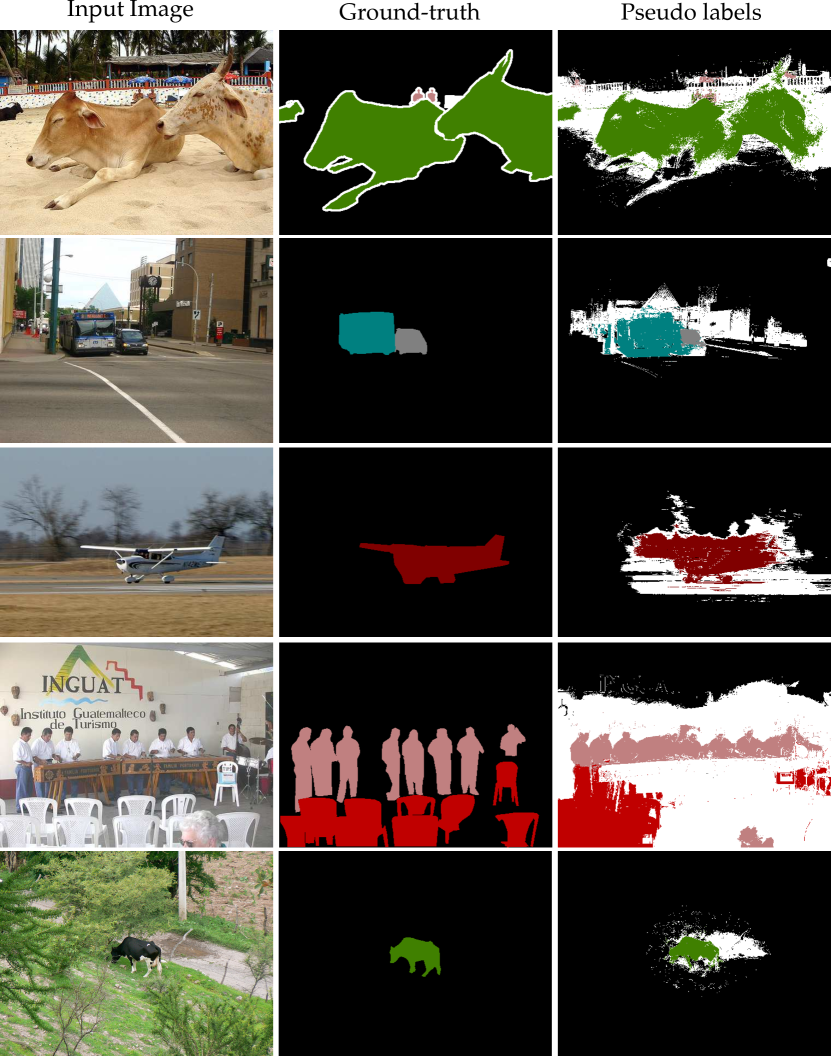
Figure 9: The generated pseudo pixel-level labels. Instances of the generated pseudo pixel-level labels from PASCAL VOC train set. The white regions correspond to the ignored pixels.

Predictions

Qualitative results of CCT on PASCAL VOC val images with different values of $n$ are presented in Fig. 10.

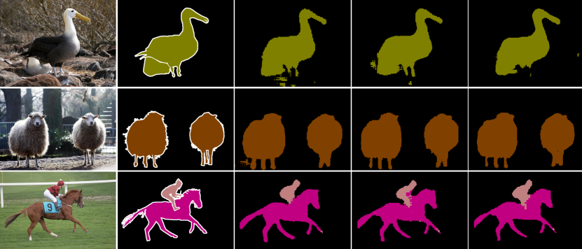
Figure 10: CCT results. Semantic Segmentation Results on the PASCAL VOC val images.

References

- [1] Jiwoon Ahn and Suha Kwak. Learning pixel-level semantic affinity with image-level supervision for weakly supervised semantic segmentation. In Proceedings of the IEEE Conference on Computer Vision and Pattern Recognition, pages 4981–4990, 2018.
- [2] Vijay Badrinarayanan, Alex Kendall, and Roberto Cipolla. Segnet: A deep convolutional encoder-decoder architecture for image segmentation. IEEE transactions on pattern analysis and machine intelligence, 39(12):2481–2495, 2017.
- [3] Shai Ben-David, John Blitzer, Koby Crammer, Alex Kulesza, Fernando Pereira, and Jennifer Wortman Vaughan. A theory of learning from different domains. Machine learning, 79(1-2):151–175, 2010.
- [4] David Berthelot, Nicholas Carlini, Ian Goodfellow, Nicolas Papernot, Avital Oliver, and Colin Raffel. Mixmatch: A holistic approach to semi-supervised learning. arXiv preprint arXiv:1905.02249, 2019.
- [5] Gabriel J Brostow, Julien Fauqueur, and Roberto Cipolla. Semantic object classes in video: A high-definition ground truth database. Pattern Recognition Letters, 30(2):88–97, 2009.
- [6] Zhangjie Cao, Lijia Ma, Mingsheng Long, and Jianmin Wang. Partial adversarial domain adaptation. In Proceedings of the European Conference on Computer Vision (ECCV), pages 135–150, 2018.
- [7] Olivier Chapelle, Bernhard Scholkopf, and Alexander Zien. Semi-supervised learning (chapelle, o. et al., eds.; 2006)[book reviews]. IEEE Transactions on Neural Networks, 20(3):542–542, 2009.
- [8] Liang-Chieh Chen, George Papandreou, Florian Schroff, and Hartwig Adam. Rethinking atrous convolution for semantic image segmentation. arXiv preprint arXiv:1706.05587, 2017.
- [9] Kevin Clark, Minh-Thang Luong, Christopher D Manning, and Quoc V Le. Semi-supervised sequence modeling with cross-view training. arXiv preprint arXiv:1809.08370, 2018.
- [10] Marius Cordts, Mohamed Omran, Sebastian Ramos, Timo Rehfeld, Markus Enzweiler, Rodrigo Benenson, Uwe Franke, Stefan Roth, and Bernt Schiele. The cityscapes dataset for semantic urban scene understanding. In Proceedings of the IEEE conference on computer vision and pattern recognition, pages 3213–3223, 2016.
- [11] Jifeng Dai, Kaiming He, and Jian Sun. Boxsup: Exploiting bounding boxes to supervise convolutional networks for semantic segmentation. 2015 IEEE International Conference on Computer Vision (ICCV), Dec 2015.
- [12] Jia Deng, Wei Dong, Richard Socher, Li-Jia Li, Kai Li, and Li Fei-Fei. Imagenet: A large-scale hierarchical image database. In 2009 IEEE conference on computer vision and pattern recognition, pages 248–255. Ieee, 2009.
- [13] Terrance DeVries and Graham W Taylor. Improved regularization of convolutional neural networks with cutout. arXiv preprint arXiv:1708.04552, 2017.
- [14] Mark Everingham, Luc Van Gool, Christopher KI Williams, John Winn, and Andrew Zisserman. The pascal visual object classes (voc) challenge. International journal of computer vision, 88(2):303–338, 2010.
- [15] Geoff French, Timo Aila, Samuli Laine, Michal Mackiewicz, and Graham Finlayson. Consistency regularization and cutmix for semi-supervised semantic segmentation. arXiv preprint arXiv:1906.01916, 2019.
- [16] Yaroslav Ganin and Victor Lempitsky. Unsupervised domain adaptation by backpropagation. arXiv preprint arXiv:1409.7495, 2014.
- [17] Yaroslav Ganin, Evgeniya Ustinova, Hana Ajakan, Pascal Germain, Hugo Larochelle, François Laviolette, Mario Marchand, and Victor Lempitsky. Domain-adversarial training of neural networks. The Journal of Machine Learning Research, 17(1):2096–2030, 2016.
- [18] Bo Geng, Dacheng Tao, and Chao Xu. Daml: Domain adaptation metric learning. IEEE Transactions on Image Processing, 20(10):2980–2989, 2011.
- [19] Yves Grandvalet and Yoshua Bengio. Semi-supervised learning by entropy minimization. In Advances in neural information processing systems, pages 529–536, 2005.
- [20] Ankur Handa, Viorica Patraucean, Vijay Badrinarayanan, Simon Stent, and Roberto Cipolla. Understanding real world indoor scenes with synthetic data. In Proceedings of the IEEE Conference on Computer Vision and Pattern Recognition, pages 4077–4085, 2016.
- [21] Bharath Hariharan, Pablo Arbeláez, Lubomir Bourdev, Subhransu Maji, and Jitendra Malik. Semantic contours from inverse detectors. In 2011 International Conference on Computer Vision, pages 991–998. IEEE, 2011.
- [22] Kaiming He, Xiangyu Zhang, Shaoqing Ren, and Jian Sun. Deep residual learning for image recognition. In Proceedings of the IEEE conference on computer vision and pattern recognition, pages 770–778, 2016.
- [23] Judy Hoffman, Dequan Wang, Fisher Yu, and Trevor Darrell. Fcns in the wild: Pixel-level adversarial and constraint-based adaptation. arXiv preprint arXiv:1612.02649, 2016.
- [24] Zilong Huang, Xinggang Wang, Jiasi Wang, Wenyu Liu, and Jingdong Wang. Weakly-supervised semantic segmentation network with deep seeded region growing. In Proceedings of the IEEE Conference on Computer Vision and Pattern Recognition, pages 7014–7023, 2018.
- [25] Wei-Chih Hung, Yi-Hsuan Tsai, Yan-Ting Liou, Yen-Yu Lin, and Ming-Hsuan Yang. Adversarial learning for semi-supervised semantic segmentation. arXiv preprint arXiv:1802.07934, 2018.
- [26] Tarun Kalluri, Girish Varma, Manmohan Chandraker, and CV Jawahar. Universal semi-supervised semantic segmentation. arXiv preprint arXiv:1811.10323, 2018.
- [27] Thomas N Kipf and Max Welling. Semi-supervised classification with graph convolutional networks. arXiv preprint arXiv:1609.02907, 2016.
- [28] Philipp Krähenbühl and Vladlen Koltun. Efficient inference in fully connected crfs with gaussian edge potentials. In Advances in neural information processing systems, pages 109–117, 2011.
- [29] Abhishek Kumar, Prasanna Sattigeri, and Tom Fletcher. Semi-supervised learning with gans: Manifold invariance with improved inference. In Advances in Neural Information Processing Systems, pages 5534–5544, 2017.
- [30] Samuli Laine and Timo Aila. Temporal ensembling for semi-supervised learning, 2016.
- [31] Dong-Hyun Lee. Pseudo-label: The simple and efficient semi-supervised learning method for deep neural networks. In Workshop on Challenges in Representation Learning, ICML, volume 3, page 2, 2013.
- [32] Jungbeom Lee, Eunji Kim, Sungmin Lee, Jangho Lee, and Sungroh Yoon. Ficklenet: Weakly and semi-supervised semantic image segmentation using stochastic inference. In Proceedings of the IEEE Conference on Computer Vision and Pattern Recognition, pages 5267–5276, 2019.
- [33] Kunpeng Li, Ziyan Wu, Kuan-Chuan Peng, Jan Ernst, and Yun Fu. Tell me where to look: Guided attention inference network. 2018 IEEE/CVF Conference on Computer Vision and Pattern Recognition, Jun 2018.
- [34] Tsung-Yi Lin, Michael Maire, Serge Belongie, James Hays, Pietro Perona, Deva Ramanan, Piotr Dollár, and C. Lawrence Zitnick. Microsoft coco: Common objects in context. Lecture Notes in Computer Science, page 740–755, 2014.
- [35] Bin Liu, Zhirong Wu, Han Hu, and Stephen Lin. Deep metric transfer for label propagation with limited annotated data. arXiv preprint arXiv:1812.08781, 2018.
- [36] John McCormac, Ankur Handa, Stefan Leutenegger, and Andrew J Davison. Scenenet rgb-d: Can 5m synthetic images beat generic imagenet pre-training on indoor segmentation? In Proceedings of the IEEE International Conference on Computer Vision, pages 2678–2687, 2017.
- [37] Takeru Miyato, Shin-ichi Maeda, Shin Ishii, and Masanori Koyama. Virtual adversarial training: a regularization method for supervised and semi-supervised learning. IEEE transactions on pattern analysis and machine intelligence, 2018.
- [38] Aude Oliva and Antonio Torralba. The role of context in object recognition. Trends in cognitive sciences, 11(12):520–527, 2007.
- [39] Avital Oliver, Augustus Odena, Colin A Raffel, Ekin Dogus Cubuk, and Ian Goodfellow. Realistic evaluation of deep semi-supervised learning algorithms. In Advances in Neural Information Processing Systems, pages 3235–3246, 2018.
- [40] George Papandreou, Liang-Chieh Chen, Kevin P Murphy, and Alan L Yuille. Weakly-and semi-supervised learning of a deep convolutional network for semantic image segmentation. In Proceedings of the IEEE international conference on computer vision, pages 1742–1750, 2015.
- [41] Adam Paszke, Sam Gross, Soumith Chintala, Gregory Chanan, Edward Yang, Zachary DeVito, Zeming Lin, Alban Desmaison, Luca Antiga, and Adam Lerer. Automatic differentiation in pytorch. 2017.
- [42] Vishal M Patel, Raghuraman Gopalan, Ruonan Li, and Rama Chellappa. Visual domain adaptation: A survey of recent advances. IEEE signal processing magazine, 32(3):53–69, 2015.
- [43] Tobias Pohlen, Alexander Hermans, Markus Mathias, and Bastian Leibe. Full-resolution residual networks for semantic segmentation in street scenes. In Proceedings of the IEEE Conference on Computer Vision and Pattern Recognition, pages 4151–4160, 2017.
- [44] Siyuan Qiao, Wei Shen, Zhishuai Zhang, Bo Wang, and Alan Yuille. Deep co-training for semi-supervised image recognition. In Proceedings of the European Conference on Computer Vision (ECCV), pages 135–152, 2018.
- [45] Antti Rasmus, Mathias Berglund, Mikko Honkala, Harri Valpola, and Tapani Raiko. Semi-supervised learning with ladder networks. In Advances in neural information processing systems, pages 3546–3554, 2015.
- [46] Fatemeh Sadat Saleh, Mohammad Sadegh Aliakbarian, Mathieu Salzmann, Lars Petersson, and Jose M Alvarez. Effective use of synthetic data for urban scene semantic segmentation. In European Conference on Computer Vision, pages 86–103. Springer, 2018.
- [47] Wenzhe Shi, Jose Caballero, Ferenc Huszár, Johannes Totz, Andrew P Aitken, Rob Bishop, Daniel Rueckert, and Zehan Wang. Real-time single image and video super-resolution using an efficient sub-pixel convolutional neural network. In Proceedings of the IEEE conference on computer vision and pattern recognition, pages 1874–1883, 2016.
- [48] Chunfeng Song, Yan Huang, Wanli Ouyang, and Liang Wang. Box-driven class-wise region masking and filling rate guided loss for weakly supervised semantic segmentation, 2019.
- [49] Shuran Song, Samuel P Lichtenberg, and Jianxiong Xiao. Sun rgb-d: A rgb-d scene understanding benchmark suite. In Proceedings of the IEEE conference on computer vision and pattern recognition, pages 567–576, 2015.
- [50] Nasim Souly, Concetto Spampinato, and Mubarak Shah. Semi supervised semantic segmentation using generative adversarial network. In Proceedings of the IEEE International Conference on Computer Vision, pages 5688–5696, 2017.
- [51] Antti Tarvainen and Harri Valpola. Mean teachers are better role models: Weight-averaged consistency targets improve semi-supervised deep learning results, 2017.
- [52] Jonathan Tompson, Ross Goroshin, Arjun Jain, Yann LeCun, and Christoph Bregler. Efficient object localization using convolutional networks. In Proceedings of the IEEE Conference on Computer Vision and Pattern Recognition, pages 648–656, 2015.
- [53] Yunchao Wei, Jiashi Feng, Xiaodan Liang, Ming-Ming Cheng, Yao Zhao, and Shuicheng Yan. Object region mining with adversarial erasing: A simple classification to semantic segmentation approach. In Proceedings of the IEEE conference on computer vision and pattern recognition, pages 1568–1576, 2017.
- [54] Yunchao Wei, Huaxin Xiao, Honghui Shi, Zequn Jie, Jiashi Feng, and Thomas S. Huang. Revisiting dilated convolution: A simple approach for weakly- and semi-supervised semantic segmentation. 2018 IEEE/CVF Conference on Computer Vision and Pattern Recognition, Jun 2018.
- [55] Qizhe Xie, Zihang Dai, Eduard Hovy, Minh-Thang Luong, and Quoc V Le. Unsupervised data augmentation. arXiv preprint arXiv:1904.12848, 2019.
- [56] Ansheng You, Xiangtai Li, Zhen Zhu, and Yunhai Tong. Torchcv: A pytorch-based framework for deep learning in computer vision. https://github.com/donnyyou/torchcv, 2019.
- [57] Hongyi Zhang, Moustapha Cisse, Yann N Dauphin, and David Lopez-Paz. mixup: Beyond empirical risk minimization. arXiv preprint arXiv:1710.09412, 2017.
- [58] Yang Zhang, Philip David, and Boqing Gong. Curriculum domain adaptation for semantic segmentation of urban scenes. In Proceedings of the IEEE International Conference on Computer Vision, pages 2020–2030, 2017.
- [59] Hengshuang Zhao, Jianping Shi, Xiaojuan Qi, Xiaogang Wang, and Jiaya Jia. Pyramid scene parsing network. In Proceedings of the IEEE conference on computer vision and pattern recognition, pages 2881–2890, 2017.
- [60] Jing Zhao, Xijiong Xie, Xin Xu, and Shiliang Sun. Multi-view learning overview: Recent progress and new challenges. Information Fusion, 38:43–54, 2017.
- [61] Bolei Zhou, Aditya Khosla, Agata Lapedriza, Aude Oliva, and Antonio Torralba. Learning deep features for discriminative localization. 2016 IEEE Conference on Computer Vision and Pattern Recognition (CVPR), Jun 2016.