A Minimal Model for Neutral Naturalness and pseudo-Nambu-Goldstone Dark Matter

Abstract

We outline a scenario where both the Higgs and a complex scalar dark matter candidate arise as the pseudo-Nambu-Goldstone bosons of breaking a global $SO(7)$ symmetry to $SO(6)$. The novelty of our construction is that the symmetry partners of the Standard Model top-quark are charged under a hidden color group and not the usual $SU(3)_{c}$. Consequently, the scale of spontaneous symmetry breaking and the masses of the top partners can be significantly lower than those with colored top partners. Taking these scales to be lower at once makes the model more natural and also reduces the induced non-derivative coupling between the Higgs and the dark matter. Indeed, natural realizations of this construction describe simple thermal WIMP dark matter which is stable under a global $U(1)_{D}$ symmetry. We show how the Large Hadron Collider along with current and next generation dark matter experiments will explore the most natural manifestations of this framework.

1 Introduction

The Standard Model (SM) of particle physics has great agreement with experiment, however it cannot be the complete theory of nature. One of the most pressing theoretical problems within the SM is the hierarchy between the weak and Planck scales. Both composite Higgs models and constructions which protect the Higgs mass through a new symmetry predict new particles or states with masses at or below the TeV scale.

Beyond this theoretical puzzle, there is overwhelming experimental evidence for dark matter (DM) which also points to new particles and interactions beyond the SM. While there is a vast and varied spectrum of possible DM candidates, weakly interacting massive particles (WIMPs) are perhaps the most theoretically compelling. This is especially the case when viewed through the lens of the hierarchy problem. Then the DM can naturally obtain a weak scale mass and couplings, providing the observed DM density through thermal freeze-out.

However, both symmetry based explanations of Higgs naturalness and thermal WIMPs have become increasingly constrained by experiment. Searches at the Large Hadron Collider (LHC) have pushed the limits on the colored symmetry partners of SM quarks to the TeV scale. At the same time a host of direct detection experiments are driving the limits on WIMP DM cross sections toward the so-called neutrino floor. With the severity of these constraints many new and interesting ideas for both Higgs naturalness and DM have been explored.

Years before the Higgs was discovered Aad:2012tfa ; Chatrchyan:2012xdj , it was pointed out that if the Higgs mass parameter is insensitive to high scales because of a new symmetry, the symmetry partners of the SM quarks do not need to carry SM color Chacko:2005pe ; Barbieri:2005ri ; Burdman:2006tz ; Poland:2008ev ; Cai:2008au . Since the discovery of colored symmetry partners to SM quarks has not followed the discovery of the Higgs, more realizations of color neutral naturalness have been explored Craig:2014aea ; Craig:2014roa ; Batell:2015aha ; Serra:2017poj ; Csaki:2017jby ; Cohen:2018mgv ; Cheng:2018gvu ; Dillon:2018wye ; Xu:2018ofw ; Serra:2019omd . Connecting DM to neutral naturalness began with the Dark Top Poland:2008ev , and has flourished in the context of twin Higgs models Garcia:2015loa ; Craig:2015xla ; Garcia:2015toa ; Farina:2015uea ; Freytsis:2016dgf ; Farina:2016ndq ; Barbieri:2016zxn ; Barbieri:2017opf ; Hochberg:2018vdo ; Cheng:2018vaj ; Terning:2019hgj ; Koren:2019iuv ; Badziak:2019zys .

In twin Higgs models, the Higgs is a pseudo-Nambu-Goldstone boson (pNGB) of a global $SO(8)$ symmetry breaking to $SO(7)$. The variety in DM candidates typically comes not from the symmetry breaking structure, but by making particular assumptions about the particle content in the twin sector. Other neutral naturalness pNGB constructions Cai:2008au ; Serra:2017poj ; Csaki:2017jby ; Xu:2018ofw ; Serra:2019omd employ smaller symmetry groups, but this move toward minimality makes it more difficult to accommodate simple DM candidates.

However, as demonstrated in Balkin:2017aep ; Balkin:2018tma , the six pNGBs that spring from $SO(7)/SO(6)$ can be associated with the Higgs doublet (respecting the custodial symmetry) along with a complex scalar DM stabilized by a global $U(1)_{D}$ . The mass of the DM and its couplings to the Higgs are determined by the symmetry breaking structure and the low energy fields that transform under the symmetry. This necessarily includes the top quark for the model to address the hierarchy problem. As a consequence, the collider bounds on colored top partners lead to couplings between the Higgs and the DM that are near or beyond the experimental limits Balkin:2017aep ; DaRold:2019ccj .

In the following section we construct a neutral natural version of the $SO(7)/SO(6)$ symmetry breaking pattern. As in other neutral natural models, the quark symmetry partners are charged under a hidden color group $SU(3)_{\widehat{c}}$ which is related to SM color by a discrete $\mathbb{Z}_{2}$ symmetry in the UV. This means they can be much lighter, allowing for additional freedom in the Higgs non-derivative coupling to the DM. These SM color neutral top partners are electroweak charged and break the DM shift symmetry, generating the DM potential. Thus, more natural top partner masses can lead to Higgs portal direct detection signals that may not be fully explored until the next generation of dark matter experiments. However, we do find that nearly all natural parameter choices lie above the neutrino floor.

In addition, the new fields related to the top quark exhibit quirky Kang:2008ea dynamics. These less studied particles can be discovered at the LHC, providing a complementary probe of the model. In Sec. 3 we outline the most promising collider searches, including both prompt and displaced signals. We find that the LHC already bounds the quirks with $U(1)_{D}$ charges. Because these particles determine the coupling between the Higgs and the dark matter, these collider bounds immediately inform the sensitivity of dark matter experiments to the pNGB WIMPs. We also calculate the corrections to the electroweak precision tests (EWPT) due to the presence of the new electroweak charged states.

In Sec. 4 we discuss the DM phenomenology, showing which parameter values lead to the correct thermal relic density and elucidate how direct and indirect searches probe the model. We find collider searches and direct detection experiments provide complementary probes, both delving into the natural parameter space along different directions in parameter space. While current limits allow versions of this framework with $\sim 10$% tuning, next generation searches should be able to discover the quirks or DM, often in multiple channels, down to $\sim 1$% tuning. Following our conclusions, in Sec. 5, we include two appendices to provide details relating to the work.

2 Neutral Naturalness from $SO(7)/SO(6)$

In this section, we describe a neutral naturalness model which includes the Higgs doublet and a complex scalar DM candidate as pNGBs. This model is related to that of the Refs. Balkin:2017aep ; Balkin:2018tma , but crucially has color neutral top partners. The global symmetry structure is $SO(7)\times U(6)$, where $U(6)\simeq SU(6)\times U(1)_{X}\supset SU(3)_{c}\times SU(3)_{\widehat{c}}\times U(1)_{X}$ includes the SM color group as well as a hidden sector color denoted $SU(3)_{\widehat{c}}$. This hidden color symmetry is assumed to be related to the SM color group by a discrete $\mathbb{Z}_{2}$ symmetry in the UV. While this discrete symmetry is broken at lower energies, this symmetry ensures that the Yukawa coupling between the Higgs and top sector runs similarly in both theories. Though this is a two-loop effect, it has been shown that, because the strong coupling is somewhat large, it can significantly affect the fine-tuning of neutral natural models Craig:2015pha .

The additional $U(1)_{X}$ ensures SM fields have their measured hypercharges. At some scale $f$ the global $SO(7)$ symmetry is broken to $SO(6)\supset SO(4)_{C}\times SO(2)_{D}\cong SU(2)_{L}\times SU(2)_{R}\times U(1)_{D}$. Here the $SO(4)_{C}\simeq SU(2)_{L}\times SU(2)_{R}$ is the familiar custodial symmetry with $SU(2)_{L}$ being the usual SM weak gauge group and $SO(2)_{D}\!=\!U(1)_{D}$ is the global symmetry that stabilizes the DM. This construction also breaks the DM’s shift symmetry in a new way. In particular, through color neutral vector-like quarks in addition to the color neutral top partners. As we see below, the DM mass and its non-derivative couplings are proportional to the masses of these color neutral vector-like quarks.

2.1 The Gauge Sector

We begin with the interactions amongst the NGBs and the gauge fields. The NGB fields can be parameterized nonlinearly as

$$\Sigma=e^{-i\Pi/f}\Sigma_{0},\hskip 28.45274pt{\rm with}\hskip 28.45274pt\Pi=\sqrt{2}\pi_{\hat{a}}T^{\hat{a}},$$ (1)

where $\Sigma_{0}=(0,0,0,0,0,0,f)^{T}$ and $T^{\hat{a}}$ are the broken generators of $SO(7)$ with $\hat{a}=1,\cdots,6$, see Appendix A for details. We immediately find

$$\Sigma=\frac{f}{|\pi|}\sin\Big{(}\frac{|\pi|}{f}\Big{)}\left(\pi_{1},\pi_{2},\pi_{3},\pi_{4},\pi_{5},\pi_{6},|\pi|\cot\Big{(}\frac{|\pi|}{f}\Big{)}\right)^{T},$$ (2)

where $|\pi|\equiv\sqrt{(\pi^{\hat{a}})^{2}}$. We can then write the leading order NGB Lagrangian as

$$\mathcal{L}_{\text{NGB}}=\frac{1}{2}\left(D_{\mu}\Sigma\right)^{T}D^{\mu}\Sigma,$$ (3)

where the covariant derivative is given by

$$D_{\mu}=\partial_{\mu}-igW^{a}_{\mu}T^{a}_{L}-ig^{\prime}B_{\mu}\left(T^{3}_{R}+X\right).$$ (4)

Note that the electric charge of fields is defined by $Q=T^{3}_{L}+T^{3}_{R}+X$, or the hypercharge is defined as $Y=T^{3}_{R}+X$.

The first four NGBs are related to the usual Higgs doublet $H=(h^{+},h^{0})^{T}$ by

$$\left(\pi_{1},\pi_{2},\pi_{3},\pi_{4}\right)=\left(-i\frac{h^{+}-h^{+\ast}}{\sqrt{2}},\frac{h^{+}+h^{+\ast}}{\sqrt{2}},i\frac{h^{0}-h^{0\ast}}{\sqrt{2}},\frac{h^{0}+h^{0\ast}}{\sqrt{2}}\right).$$ (5)

In unitary gauge when $h^{+}=0$ and $h^{0}=\overline{h}/\sqrt{2}$ we have

$$\left(\pi_{1},\pi_{2},\pi_{3},\pi_{4},\pi_{5},\pi_{6}\right)=\left(0,0,0,\overline{h},\sqrt{2}\,\text{Im}\chi,\sqrt{2}\,\text{Re}\chi\right),$$ (6)

where we have defined $\chi=(\pi_{6}+i\pi_{5})/\sqrt{2}$ as a complex scalar which is our DM candidate. It is convenient to make the field redefinition Gripaios:2009pe ,

$$\sin\left(\frac{|\pi|}{f}\right)\frac{\pi^{a}}{|\pi|}\to\frac{\pi^{a}}{f}.$$ (7)

We can then write NGB field as

$$\Sigma=\left(0,0,0,\overline{h},\sqrt{2}\,\text{Im}\chi,\sqrt{2}\,\text{Re}\chi,\sqrt{f^{2}-\overline{h}^{2}-2|\chi^{2}|}\,\right),$$ (8)

in unitary gauge. The NGB Lagrangian has the leading order terms

$$\mathcal{L}_{\text{NGB}}= \frac{1}{2}\left(\partial_{\mu}\overline{h}\right)^{2}+\left|\partial_{\mu}\chi\right|^{2}+\frac{1}{2}\frac{\left(\overline{h}\partial_{\mu}\overline{h}+\chi^{\ast}\partial_{\mu}\chi+\chi\partial_{\mu}\chi^{\ast}\right)^{2}}{f^{2}-\overline{h}^{2}-2|\chi^{2}|}$$

$$+\frac{\overline{h}^{2}}{4}\left[g^{2}W^{+\mu}W^{-}_{\mu}+\frac{1}{2}\left(gW^{3}_{\mu}-g^{\prime}B_{\mu}\right)^{2}\right].$$ (9)

When $\overline{h}$ gets a vacuum expectation value (VEV) of $v\approx 246$ GeV we write

$$\overline{h}=v+c_{v}h,\ \ \ \ \text{with}\ \ \ \ c_{v}\equiv\sqrt{1-\tfrac{v^{2}}{f^{2}}},$$ (10)

to ensure that $h$ is canonically normalized. We also define $s_{v}\equiv v/f$.

2.2 The Quark Sector

The quark fields include particles charged under both SM color and the hidden color group. In terms of $SO(7)$ and $SU(6)$ representations we have the left- and right-handed quarks as ${\cal Q}_{L}=({\bf 7,6})$ and ${\cal T}_{R}=({\bf 1,6})$. These can be split up schematically in terms of fields in the ${\bf 3}$ of their respective color groups

$$\mathcal{Q}_{L}=(Q_{L},\widehat{Q}_{L}),\ \ \ \ {\cal T}_{R}=(t_{R},\widehat{T}_{R}),$$ (11)

where we have put a hat on fields charged under the hidden color group. More explicitly we write out the low lying left-handed fields as

$$\sqrt{2}{\cal Q}_{L}=\blockarray{lcc}&SU(3)_{c}SU(3)_{\widehat{c}}\\ \block{l(c|c)}\hbox{\multirowsetup$SO(4)_{C}$}ib_{L}i\widehat{b}_{L}\\ b_{L}\widehat{b}_{L}\\ it_{L}i\widehat{t}_{L}\\ -t_{L}-\widehat{t}_{L}\\ \BAhhline{--}\hbox{\multirowsetup$U(1)_{D}$}0\displaystyle i\widehat{X}_{L}-i\widehat{Y}_{L}\\ 0\widehat{X}_{L}+\widehat{Y}_{L}\\ \BAhhline{--}0\displaystyle\sqrt{2}\widehat{T}_{L}\\ \;\;,$$ (12)

where $q_{L}=(t_{L},b_{L})^{T}$ is the usual $SU(2)_{L}$ quark doublet. This is similar in spirit to Refs. Balkin:2017aep ; Serra:2017poj ; Csaki:2017jby which use incomplete quark multiplets. One can imagine the other fields lifted out of the low energy spectrum by vector-like masses, or as in extra dimensional models Burdman:2006tz ; Cai:2008au that the boundary conditions of the bulk fields are such that the zero modes vanish. In order to obtain the correct hypercharge for $t_{L}$, $t_{R}$, and $b_{L}$, both $\mathcal{Q}_{L}$ and $\mathcal{T}_{R}$ have a $U(1)_{X}$ charge of 2/3. The Yukawa coupling term $\overline{\mathcal{Q}}_{L}\Sigma\mathcal{T}_{R}$ then implies that the NGBs have zero $X$ charge, which in particular implies that $\chi$ has no SM gauge charges.

The top sector couplings follow from

$$\mathcal{L} \supset\lambda_{t}\overline{\mathcal{Q}}_{L}\Sigma\mathcal{T}_{R}+\text{h.c.}$$ (13)

$$=\lambda_{t}\!\left[\!-\!\left(\overline{q}_{L}t_{R}+\overline{\widehat{q}}_{L}\widehat{T}_{R}\right)\widetilde{H}\!+\!\chi^{\ast}\overline{\widehat{X}}_{L}\widehat{T}_{R}\!+\!\chi\overline{\widehat{Y}}_{L}\widehat{T}_{R}\!+\!f\Big{(}1-\frac{|H|^{2}+|\chi|^{2}}{f^{2}}+\ldots\Big{)}\overline{\widehat{T}}_{L}\widehat{T}_{R}\right]\!+\!\text{h.c.},$$

where $q_{L}\!=\!(t_{L},b_{L})^{T}$ and $\widehat{q}_{L}\!=\!(\widehat{t}_{L},\widehat{b}_{L})^{T}$ are $SU(2)_{L}$ doublets and we have restored the eaten NGBs for the moment into the Higgs doublet $H$, and defined $\widetilde{H}=i\sigma^{2}H^{\ast}$. From these interactions we obtain the one-loop diagrams in Fig. 1 relevant to the mass corrections for $H$ and $\chi$. The leading contributions from the top quark are doubled by $\widehat{q}_{L}$ interaction, but this combination is exactly cancelled by $\widehat{T}_{L}$. Like in Xu:2018ofw , the contributions from fields carrying SM color and those carrying hidden color are not equal. Note that the DM shift symmetry is broken by the SM color neutral top partner $\widehat{T}$ and $U(1)_{D}$ charged fermions $\widehat{X}_{L},\widehat{Y}_{L}$.

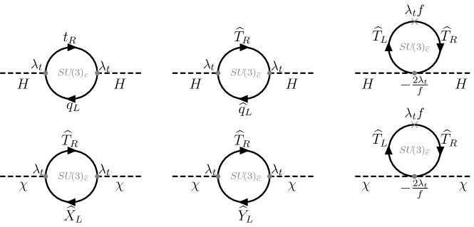
Figure 1: These Feynman diagrams show cancelation of quadratic divergences due to $SU(3)_{c}$ top quark and $SU(3)_{\widehat{c}}$ top quark for the SM-like Higgs $H$ (upper row) and the complex scalar $\chi$ (lower row).

The hidden color fields can be lifted through vector-like mass terms with new heavy states. We can write down the mass terms

$$\mathcal{L}_{\text{vec mass}}=-m_{Q}\overline{\widehat{q}}_{L}\widehat{q}_{R}-m_{X}\overline{\widehat{X}}_{L}\widehat{X}_{R}-m_{Y}\overline{\widehat{Y}}_{L}\widehat{Y}_{R}+\text{h.c.}~{},$$ (14)

where $\widehat{q}_{R}=(\widehat{t}_{R},\widehat{b}_{R})^{T}$ is an $SU(2)_{L}$ doublet. We take these to be free parameters as we calculate the scalar potential.

2.3 The Scalar Potential

We are interested in the obtaining the potentials for both the Higgs and the DM. This is obtained from the Coleman-Weinberg (CW) potential Coleman:1973jx

$$V_{\text{CW}}=-\frac{N_{c}}{8\pi^{2}}\Lambda_{\text{UV}}^{2}\text{Tr}\mathcal{M}^{2}-\frac{N_{c}}{16\pi^{2}}\text{Tr}\left[\mathcal{M}^{4}\left(\ln\frac{\mathcal{M}^{2}}{\Lambda_{\text{UV}}^{2}}-\frac{1}{2}\right)\right],$$ (15)

where $\mathcal{M}^{2}$ is the Dirac fermion mass squared matrices, with masses as functions of $\overline{h}$ and $\chi$. We note first that there is no quadratic sensitivity to to the cut off because $\text{Tr}\,\mathcal{M}^{2}$ is independent of the scalar fields. However, we do find logarithmic sensitivity because

$$\text{Tr}\,\mathcal{M}^{4}=\frac{\lambda_{t}^{4}}{2}\overline{h}^{4}+\overline{h}^{2}\lambda_{t}^{2}\left(m_{Q}^{2}-\lambda_{t}^{2}f^{2}\right)+2\lambda_{t}^{2}|\chi|^{2}\left(m_{X}^{2}+m_{Y}^{2}\right),$$ (16)

where we have dropped field independent terms.

Any remaining terms in the scalar potential, such as quartic mixing of $\overline{h}$ and $\chi$ or a $|\chi|^{4}$ term, are independent of $\Lambda_{\text{UV}}$ and so are robustly determined by the low energy physics. Clearly, in order for electroweak symmetry to break we need the Higgs mass parameter to be negative, so we require $f\lambda_{t}>m_{Q}$. From Eq. (10) we see that Higgs couplings to SM fields will be reduced by $c_{v}$. As in other pNGB Higgs construction, this implies that $f$ exceeds $v$ by a factor of a few. As in Xu:2018ofw we find there must be a cancellation between independent terms ($m_{Q}$ and $\lambda_{t}f$) to obtain the correct Higgs mass. This motivates defining

$$\lambda_{t}^{2}f^{2}\equiv m_{Q}^{2}(1+\delta_{m}).$$ (17)

For simplicity, in this work we take the vector-like masses of the DM sector to be equal

$$m_{X}=m_{Y}\equiv m_{V}.$$ (18)

This mass scale is related to $m_{Q}$ by the ratio $r_{Q}=m^{2}_{V}/m^{2}_{Q}$. In this limit we find one of the dark fermion mass eigenstates is exactly $m_{V}$, while the others are determined by a cubic equation. We then find the scalar potential, which has the general form of

$$V(h,\chi)=\frac{1}{2}\mu_{h}^{2}\overline{h}^{2}+\frac{\lambda_{h}}{4}\overline{h}^{4}+\mu^{2}_{\chi}|\chi|^{2}+\lambda_{\chi}|\chi|^{4}+\lambda_{h\chi}\overline{h}^{2}|\chi|^{2}~{}.$$ (19)

The potential parameters are calculated from the CW potential in Eq. (15). We find

$$\mu_{h}^{2} =\frac{3\lambda_{t}^{2}}{8\pi^{2}}\bigg{[}m_{Q}^{2}\ln\frac{\Lambda_{\text{UV}}^{2}}{m_{Q}^{2}}-\lambda_{t}^{2}f^{2}\ln\frac{\Lambda_{\text{UV}}^{2}}{\lambda_{t}^{2}f^{2}}+\frac{\lambda_{t}^{2}f^{2}\,m_{Q}^{2}}{m_{Q}^{2}-\lambda_{t}^{2}f^{2}}\ln\frac{\lambda_{t}^{2}f^{2}}{m_{Q}^{2}}\bigg{]},$$ (20)

$$\lambda_{h} =\frac{3\lambda_{t}^{4}}{16\pi^{2}}\bigg{[}\ln\frac{\Lambda_{\text{UV}}^{4}}{\lambda_{t}^{2}f^{2}\frac{\lambda_{t}^{2}}{2}\overline{h}^{2}}-\frac{1}{2}\frac{\big{(}3m_{Q}^{2}-\lambda_{t}^{2}f^{2}\big{)}^{2}}{\big{(}m_{Q}^{2}-\lambda_{t}^{2}f^{2}\big{)}^{2}}-m_{Q}^{4}\frac{3m_{Q}^{2}-\lambda_{t}^{2}f^{2}}{\big{(}m_{Q}^{2}-\lambda_{t}^{2}f^{2}\big{)}^{3}}\ln\frac{\lambda_{t}^{2}f^{2}}{m_{Q}^{2}}\bigg{]},$$ (21)

$$\mu_{\chi}^{2} =\frac{3\lambda_{t}^{2}m_{V}^{2}}{4\pi^{2}}\bigg{[}\ln\frac{\Lambda_{\text{UV}}^{2}}{\lambda_{t}^{2}f^{2}}+\frac{m_{V}^{2}}{m_{V}^{2}-\lambda_{t}^{2}f^{2}}\ln\frac{\lambda_{t}^{2}f^{2}}{m_{V}^{2}}\bigg{]},$$ (22)

$$\lambda_{\chi} =-\frac{3\lambda_{t}^{4}m_{V}^{4}}{4\pi^{2}\big{(}m_{V}^{2}-\lambda_{t}^{2}f^{2}\big{)}^{2}}\bigg{[}2+\frac{m_{V}^{2}+\lambda_{t}^{2}f^{2}}{m_{V}^{2}-\lambda_{t}^{2}f^{2}}\ln\frac{\lambda_{t}^{2}f^{2}}{m_{V}^{2}}\bigg{]},$$ (23)

$$\lambda_{h\chi} =-\frac{3\lambda_{t}^{4}m_{V}^{2}}{8\pi^{2}}\bigg{[}\frac{2m_{Q}^{2}-\lambda_{t}^{2}f^{2}}{(m_{Q}^{2}-\lambda_{t}^{2}f^{2})(m_{V}^{2}-\lambda_{t}^{2}f^{2})}+\frac{m_{V}^{2}\big{(}2m_{Q}^{2}-m_{V}^{2}\big{)}}{\big{(}m_{V}^{2}-\lambda_{t}^{2}f^{2}\big{)}^{2}(m_{Q}^{2}-m_{V}^{2})}\ln\frac{\lambda_{t}^{2}f^{2}}{m_{V}^{2}}$$

$$\hskip 56.9055pt-\frac{m_{Q}^{4}}{\big{(}m_{Q}^{2}-\lambda_{t}^{2}f^{2}\big{)}^{2}(m_{Q}^{2}-m_{V}^{2})}\ln\frac{\lambda_{t}^{2}f^{2}}{m_{Q}^{2}}\bigg{]}.$$ (24)

We need the dark $U(1)_{D}$ to remain unbroken so that $\chi$ is stable. This means we are interested in vacua with $\langle\chi\rangle=0$ and $\langle\overline{h}\rangle=v$. With $\mu_{h}^{2}<0$ and $\mu_{\chi}^{2}>0$, this is the deepest vacuum as long as $\lambda_{h}\lambda_{\chi}<\lambda_{h\chi}^{2}$. However, when $\lambda_{h}\lambda_{\chi}>\lambda_{h\chi}^{2}$ the vacuum with $\langle\chi\rangle\neq 0$ becomes a saddle point rather than a minimum, so the deepest stable vacuum still has $\langle\chi\rangle=0$. In this case we find

$$\mu_{h}^{2}=-\lambda_{h}v^{2},\hskip 28.45274ptm_{h}^{2}=2c_{v}^{2}\lambda_{h}v^{2},\hskip 28.45274ptm_{\chi}^{2}=\mu_{\chi}^{2}+\lambda_{h\chi}v^{2}.$$ (25)

Since we know $v\simeq 246$ GeV and the Higgs mass $m_{h}\simeq 125$ GeV, therefore $\lambda_{h}\simeq 0.13$ and $\mu_{h}\simeq 89$ GeV. The constraints on Higgs couplings (see Sec. 3) imply that $f\gtrsim 3v$, which means $\delta_{m}\ll 1$. It then makes sense to expand the potential terms to leading order in $\delta_{m}$. We find

$$\mu_{h}^{2} =-\frac{3\lambda_{t}^{2}}{8\pi^{2}}m_{Q}^{2}+\mathcal{O}(\delta_{m}),\hskip 28.45274pt\lambda_{h}=\frac{3\lambda_{t}^{4}}{16\pi^{2}}\bigg{[}\frac{2}{3}+\ln\frac{\Lambda_{\text{UV}}^{4}}{m_{Q}^{2}\frac{\lambda_{t}^{2}}{2}\overline{h}^{2}}+\mathcal{O}(\delta_{m})\bigg{]},$$ (26)

$$\mu_{\chi}^{2} =\frac{3\lambda_{t}^{2}m_{V}^{2}}{4\pi^{2}}\bigg{[}\ln\frac{\Lambda_{\text{UV}}^{2}}{m_{Q}^{2}}+\frac{r_{Q}}{1-r_{Q}}\ln r_{Q}+\mathcal{O}(\delta_{m})\bigg{]},$$ (27)

$$\lambda_{\chi} =\frac{3\lambda_{t}^{4}r_{Q}^{2}}{4\pi^{2}\left(1-r_{Q}\right)^{2}}\bigg{[}\frac{1+r_{Q}}{1-r_{Q}}\ln\frac{1}{r_{Q}}-2+\mathcal{O}(\delta_{m})\bigg{]},$$ (28)

$$\lambda_{h\chi} =\frac{3\lambda_{t}^{4}r_{Q}}{8\pi^{2}(1-r_{Q})^{2}}\bigg{[}\frac{3-r_{Q}}{2}-\frac{r_{Q}(2-r_{Q})}{1-r_{Q}}\ln\frac{1}{r_{Q}}+\mathcal{O}(\delta_{m})\bigg{]}.$$ (29)

Here we have taken $\ln\frac{\Lambda_{\text{UV}}^{2}}{m_{Q}^{2}}$ to be order one, as expected for a cutoff of a few TeV.

The Higgs potential has logarithmic dependence on $\Lambda_{\text{UV}}$. This is similar to both the Twin Higgs Contino:2017moj and $SO(6)/SO(5)$ constructions Serra:2017poj where sizable UV contributions lead to the correct Higgs mass. In the limit of small $\delta_{m}$ and taking $\lambda_{t}^{\overline{\text{MS}}}=0.936$ we find $\mu^{2}_{h}\approx-(146)^{2}$ $\text{GeV}^{2}$ and $\lambda_{h}\approx 0.13$ for $m_{Q}=800$ GeV and $\Lambda_{\text{UV}}=3$ TeV. These are similar to the SM listed above, so we expect that a suitable UV completion, perhaps composite or holographic, can easily accommodate the measured Higgs mass.

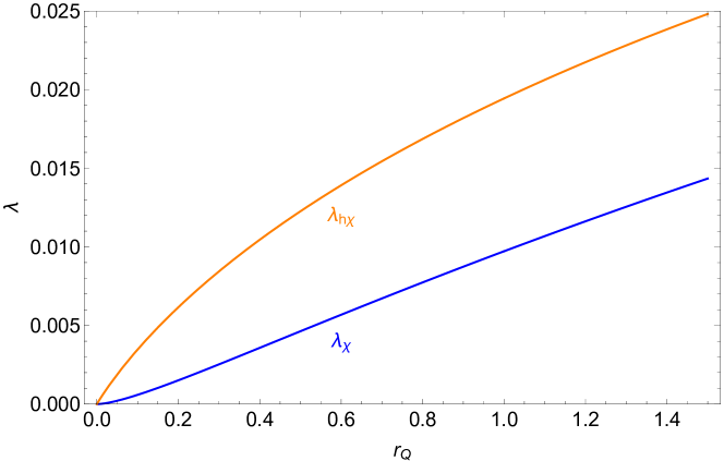
Figure 2: The quartic couplings involving the DM field $\chi$ as a function of $r_{Q}=m_{V}^{2}/m_{Q}^{2}$. We have neglected all terms of order $\delta_{m}$.

At the same time the quartic couplings that involve $\chi$ are determined completely by the low-energy theory. Thus, we can make robust predictions about the DM without knowledge of the UV completion. In Fig. 2 we see that these quartics are order $10^{-2}$ over a wide span of $r_{Q}$. This gives the value of the DM self-interactions as well as its coupling strength to the Higgs. The value of $r_{Q}$ is constrained by collider production of the hidden color fermions which is taken up in the following section.

2.3.1 Tuning

The Higgs potential obtained above also allows us to determine tuning of the Higgs mass parameter. We use the formula

$$\Delta=\left|\frac{2\delta\mu^{2}}{m_{h}^{2}}\right|^{-1},$$ (30)

where $\delta\mu^{2}$ is the leading one-loop correction to the Higgs mass parameter

$$\delta\mu^{2}=\frac{N_{c}}{8\pi^{2}}\lambda_{t}^{2}\left(m_{Q}^{2}-\lambda_{t}^{2}f^{2}\right)\ln\frac{\Lambda^{2}_{\text{UV}}}{m_{Q}^{2}}=-\frac{3\lambda_{t}^{2}\delta_{m}}{8\pi^{2}}m_{Q}^{2}\ln\frac{\Lambda^{2}_{\text{UV}}}{m_{Q}^{2}}.$$ (31)

Clearly, this tuning depends sensitively on $\delta_{m}$, and is greatly reduced when $\delta_{m}\ll 1$.

It is useful to connect $\delta_{m}$ to $v/f$. This is done by simply minimizing the part of the Higgs potential that depends on $\ln\Lambda_{\text{UV}}$. This leads to the relation

$$\frac{v^{2}}{f^{2}}=1-\frac{m_{Q}^{2}}{\lambda_{t}^{2}f^{2}}=\frac{\delta_{m}}{1+\delta_{m}},$$ (32)

similar to what was found in Xu:2018ofw . We rewrite this as

$$\delta_{m}=\frac{v^{2}/f^{2}}{1-v^{2}/f^{2}},$$ (33)

to see that $\delta_{m}$ roughly tracks the tuning required to misalign the vacuum, as it should, for it is by choosing $\delta_{m}$ small that we obtain the correct Higgs mass. This makes clear that taking $\delta_{m}$ small is not an additional tuning, but the only tuning required to realize the correct Higgs potential. For instance, when $f\!/\!v=3$ (10) we find $\delta_{m}\approx 0.125$ (0.01) which corresponds to $\sim$10% (1%) tuning.

3 Collider phenomenology

The collider signals of this model arise from the Higgs sector and the production and decay of the hidden color quirks. To determine both these effects we need the physical mass states of the hidden sector fermions. The relevant mass matrix $\mathcal{M}_{F}$ is

$$-\left(\widehat{t}_{L},\;\widehat{T}_{L}\right)\mathcal{M}_{F}\left(\begin{array}[]{c}\widehat{t}_{R}\\ \widehat{T}_{R}\end{array}\right)=-\left(\widehat{t}_{L},\;\widehat{T}_{L}\right)\left(\begin{array}[]{cc}m_{Q}&m_{t}\\ 0&-c_{v}\lambda_{t}f\end{array}\right)\left(\begin{array}[]{c}\widehat{t}_{R}\\ \widehat{T}_{R}\end{array}\right).$$ (34)

As noted in the previous section to obtain the correct Higgs mass without introducing additional fine-tuning, we require,

$$m_{Q}=\frac{\lambda_{t}f}{\sqrt{1+\delta_{m}}}=c_{v}\lambda_{t}f,$$ (35)

where $\delta_{m}$ is given in Eq. (33). In the following, we fix the vector-like mass for the quirk doublet $m_{Q}$ to the this value. Note that we can use this relation to define $f\!/\!v$ in terms of $m_{Q}$:

$$\frac{f}{v}=\sqrt{1+\frac{m_{Q}^{2}}{2m_{t}^{2}}}.$$ (36)

The physical masses are obtained by diagonalizing the fermion mass matrix by the transformation $R(\theta_{L})^{T}\mathcal{M}_{F}R(\theta_{R})$, where the rotation matrices are

$$R(\theta_{i})=\left(\begin{array}[]{cc}\cos\theta_{i}&\sin\theta_{i}\\ \!\!\!-\sin\theta_{i}&\cos\theta_{i}\end{array}\right).$$ (37)

The mass eigenvalues are given by

$$m^{2}_{\pm}=m_{Q}^{2}\left(1+\frac{m_{t}^{2}}{2m_{Q}^{2}}\pm\frac{m_{t}}{m_{Q}}\sqrt{1+\frac{m_{t}^{2}}{4m_{Q}^{2}}}\right),$$ (38)

and the mixing angles are

$$\sin 2\theta_{L}=-\sin 2\theta_{R}=\frac{1}{\sqrt{1+\frac{m_{t}^{2}}{4m_{Q}^{2}}}}~{}.$$ (39)

In other words, $\theta_{L}=-\theta_{R}\equiv\theta$. The unmixed states are described by Dirac fermions $\widehat{T}_{\pm}$ with masses $m_{\pm}$, their couplings to SM fields are given in Appendix B.

3.1 Scalar Sector

Like other pNGB Higgs models we find the tree level couplings of the Higgs to SM states are reduced. In our case they are reduced by $c_{v}$, which follows immediately from Eq. (10). This leads to the usual bound of $f\gtrsim 3v$ from the LHC measurement of Higgs couplings to gauge bosons. It may also lead to interesting signals at the HL-LHC and future colliders. At the same time, the existence of new fermionic states with electric charge that couple to the Higgs amplifies its coupling to photons. As in the quirky little Higgs model Cai:2008au , this pushes the rate of $h\to\gamma\gamma$ closer to the SM prediction Burdman:2014zta .

Explicitly, we find the Higgs width into diphotons is approximately

$$\Gamma(h\to\gamma\gamma)=\frac{\alpha^{2}m_{h}^{3}}{256\pi^{3}v^{2}} \left|c_{v}\left[A_{V}\left(\frac{4m_{W}^{2}}{m_{h}^{2}}\right)+\frac{4}{3}A_{F}\left(\frac{4m_{t}^{2}}{m_{h}^{2}}\right)\right]\right.$$

$$+\frac{m_{t}\sin\theta}{m_{+}}\left(c_{v}\cos\theta-\sqrt{2}s_{v}\sin\theta\right)\frac{4}{3}A_{F}\left(\frac{4m_{+}^{2}}{m_{h}^{2}}\right)$$

$$\left.+\frac{m_{t}\cos\theta}{m_{-}}\left(c_{v}\sin\theta+\sqrt{2}s_{v}\cos\theta\right)\frac{4}{3}A_{F}\left(\frac{4m_{-}^{2}}{m_{h}^{2}}\right)\right|^{2}.$$ (40)

In Fig. 3 we see how the production of a given Higgs to SM final state rate changes relative to the SM prediction as a function of $m_{Q}$. The blue curve shows the usual result for tree level Higgs coupling deviations, while the dashed orange curve denotes the decay into two photons. We see that the latter is slightly increased relative to the other rates. However, the deviation is small enough that it would likely require a future lepton collider to measure it Fujii:2017vwa ; deBlas:2018mhx ; Abada:2019lih . Current Higgs coupling measurements require this ratio be no less than $0.8$, and the HL-LHC is expected to reach a precision corresponding to about $0.9$ Cepeda:2019klc . We see that these already begin to probe $v/f$, but do not reach beyond about 10% tuning.

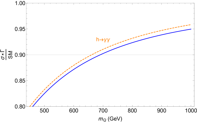
Figure 3: Ratio of the production of a the Higgs boson and subsequent prompt decay into SM final states as a function of $m_{Q}$. The $h\to\gamma\gamma$ line is given by the dashed orange curve, while all other prompt SM final states fall along the solid blue curve.

The Higgs also develops a loop level coupling to the gluons of the hidden QCD. Similar to coupling to the photon, we find the Higgs coupling to hidden gluons takes the form

$$c_{\widehat{g}}\frac{\widehat{\alpha}_{s}}{12\pi}\frac{h}{v}\widehat{G}^{a}_{\mu\nu}\widehat{G}^{a\mu\nu},$$ (41)

where $\widehat{\alpha}_{s}=\widehat{g}^{2}_{s}/(4\pi)$ is the hidden sector strong coupling parameter, $\widehat{G}^{a}_{\mu\nu}$ is the hidden gluon field strength, and

$$c_{\widehat{g}} =\frac{m_{t}\sin\theta}{m_{+}}\left(c_{v}\cos\theta-\sqrt{2}s_{v}\sin\theta\right)\frac{3}{4}A_{F}\left(\frac{4m_{+}^{2}}{m_{h}^{2}}\right)$$

$$\quad+\frac{m_{t}\cos\theta}{m_{-}}\left(c_{v}\sin\theta+\sqrt{2}s_{v}\cos\theta\right)\frac{3}{4}A_{F}\left(\frac{4m_{-}^{2}}{m_{h}^{2}}\right).$$ (42)

This leads to the Higgs width into hidden gluons

$$\Gamma(h\to\widehat{g}\widehat{g})=\frac{\widehat{\alpha}_{s}m_{h}^{5}}{288\pi^{3}v^{2}}|c_{\widehat{g}}|^{2},$$ (43)

which may contribute to a detectable Higgs width at future lepton colliders.

Since the states charged with hidden color carry $U(1)_{X}$ charge, they are electrically charged under the SM. Bounds from LEP imply that such states cannot be lighter than about 100 GeV. Consequently, the lightest hadrons of the hidden confining group are the glueballs. The lightest glueball state is a $0^{++}$ and has a small mixing with the Higgs. This allows the glueballs to decay with long lifetime to SM states. From Juknevich:2009gg we find the glueball partial width into SM states to be

$$\Gamma\left(0^{++}\to X_{\text{SM}}X_{\text{SM}}\right)=|c_{\widehat{g}}|^{2}\left[\frac{\widehat{\alpha}_{s}}{6\pi v}\frac{f_{0^{++}}}{m_{h}^{2}-m_{0}^{2}}\right]^{2}\Gamma_{\text{SM}}\left(h(m_{0})\to X_{\text{SM}}X_{\text{SM}}\right)$$ (44)

where $m_{0}$ is the mass of the lightest glueball, $f_{0^{++}}=\langle 0|\text{Tr}\,\widehat{G}_{\mu\nu}\widehat{G}^{\mu\nu}|0^{++}\rangle$, and $\Gamma\left(h(m_{0})\to X_{\text{SM}}X_{\text{SM}}\right)$ is the SM Higgs partial width for a Higgs with mass $m_{0}$. Lattice calculations have determined $4\pi\widehat{\alpha}_{s}f_{0^{++}}=3.1m_{0}^{3}$ Chen:2005mg . In addition, the exotic decays of the Higgs into glueballs with displaced decays can lead to striking signals at the LHC Curtin:2015fna .

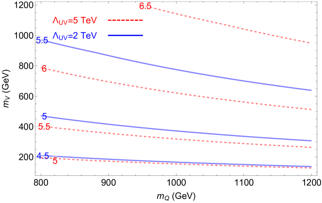
Figure 4: Contours of the hidden color $\widehat{\Lambda}_{\text{QCD}}$ as a function of the vector-like masses of hidden color fermions. The blue solid (red dashed) contours correspond to a UV cutoff $\Lambda_{\rm UV}\!=\!2(5)\;\hbox{TeV}$ where the SM and hidden strong couplings become equal.

To be more precise we must estimate the mass of the hidden glueball. This is done by estimating the hidden scale $\widehat{\Lambda}_{\text{QCD}}$ using two-loop running. We assume at scales near the cutoff of a few TeV the SM and hidden strong couplings become equal because of the $\mathbb{Z}_{2}$ symmetry in the UV. Thus, we can run the SM strong coupling up to the cutoff and then run the hidden coupling down from the cutoff for a given spectrum. In Fig. 4 we find that the hidden color strong scale varies between about 4.5 to 6.5 GeV for $m_{Q}\in[800,1200]\;\hbox{GeV}$. This implies the lightest glueball mass, taken to be about $6.8\widehat{\Lambda}_{\text{QCD}}$, is likely to fall between 30 and 45 GeV. Then using the glueball decay width in Eq. (44) we find the glueballs typically have a decay length of hundreds of meters, with the smallest values for larger $m_{V}$ and $\Lambda_{\text{UV}}$. The displaced decays from these particles may be quite challenging for the ATLAS and CMS to detect, but may be detected by MATHUSLA-like detectors Curtin:2018mvb .

There may also be new scalars related to the spontaneous symmetry breaking mechanism. In weakly coupled UV completions there may be a radial mode, a scalar whose mass close to $f$. As has been detailed for other pNGB realizations of neutral naturalness Craig:2015pha ; Buttazzo:2015bka ; Ahmed:2017psb ; Chacko:2017xpd ; Kilic:2018sew ; Alipour-fard:2018mre , this scalar will have order one couplings to all the pNGBs, leading to observable signals at the LHC and future colliders. If the UV completion involves an approximate scale symmetry then a heavy scalar associated with the breaking of scale invariance, the dilaton, can have large coupling to the SM and hidden sector states Ahmed:2019kgl providing additional collider signals.

3.2 Electroweak Precision Tests

Extensions of the SM are constrained by precision electroweak measurements. The constraints can be expressed in terms of the oblique parameters $S$, $T$, and $U$ Peskin:1990zt ; Peskin:1991sw . The contributions to $U$ are typically small, so we only compute the contribution to $S$ and $T$. These contributions arise from the new electroweak charged fermions inducing important radiative corrections to gauge boson propagators. In addition, the modified coupling of the Higgs boson to gauge bosons leads to an infrared log divergence Contino:2010rs . We find the leading contributions to be

$$S\approx \frac{2N_{\widehat{c}}\,m_{t}^{2}}{15\pi\,m_{Q}^{2}}+\frac{1}{12\pi}\frac{v^{2}}{f^{2}}\ln{\left(\frac{\Lambda^{2}_{\rm UV}}{m_{h}^{2}}\right)},$$ (45)

$$T\approx \frac{13N_{\widehat{c}}\,m_{t}^{4}}{120\pi m_{Z}^{2}m^{2}_{Q}\sin^{2}2\theta_{W}}-\frac{3}{16\pi}\frac{1}{\cos^{2}\theta_{W}}\frac{v^{2}}{f^{2}}\ln{\left(\frac{\Lambda_{\rm UV}^{2}}{m_{h}^{2}}\right)},$$ (46)

where $\Lambda_{\rm UV}$ is UV cutoff scale, $\theta_{W}$ is the usual weak mixing angle, and the factor of $N_{\widehat{c}}$ comes from the number of dark QCD color.

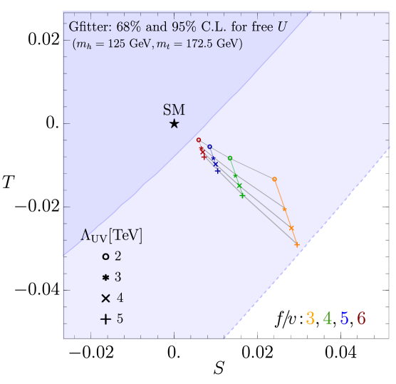
Figure 5: The allowed region in the $S\!-\!T$ plane leaving the $U$ parameter free Haller:2018nnx . The colored points (orange, green, blue, and red) indicate the values of $S$ and $T$ for $f\!/\!v=3,4,5,6$ with UV cutoff scale $2,3,4,5$ TeV.

.

As expected, the contributions from vector-like fermions, $\widehat{X}$ and $\widehat{Y}$, cancel as well as the power law UV divergences. These contributions are compared to the experimental fits and found to lie within the $68\%$ and $95\%$ allowed regions as provided by the Gfitter collaboration Haller:2018nnx . In Fig. 5, we plot $S$ and $T$ with $U$ free, for the input parameters $m_{h}=125$ GeV and $m_{t}=172.5$ GeV. The colored points in the figure correspond to values of $f\!/\!v=3,4,5,6$ (orange, green, blue, and red) and $\Lambda_{\text{UV}}$, 2, 3, 4, 5 TeV. With increasing the value of $f$, the value of $S$ and $T$ approach the SM value.

3.3 Quirky Signals

The new fermions ($\widehat{T}_{\pm}$, $\widehat{X}$, and $\widehat{Y}$) can be produced at colliders through Drell-Yan due to their hypercharge of 2/3. We parameterize the couplings of any fermion $f$ to the $Z$ boson and the photon by

$$\mathcal{L}\supset\frac{g}{2c_{W}}Z_{\mu}\overline{f}\gamma^{\mu}(v_{f}-a_{f}\gamma^{5})f+eQ_{f}A_{\mu}\overline{f}\gamma^{\mu}f,$$ (47)

where $c_{W}$ and $s_{W}$ is the cosine and sine of the weak mixing angle while $g$ and $e=gs_{W}$ are the weak and electric couplings, respectively. As an example, SM fermions have $v_{f}=T_{3}-2Qs_{W}^{2}$ and $a_{f}=T_{3}$. We then find the partonic cross section for $\overline{q}q\to Z,\gamma\to\overline{f}f$ to be

$$\sigma(\overline{q}q\to\overline{f}f)(\tilde{s})= \frac{\pi\alpha_{Z}^{2}N_{\widehat{c}}}{12N_{c}\tilde{s}(1-m_{Z}^{2}/\tilde{s})^{2}}\sqrt{1-\frac{4m_{f}^{2}}{\tilde{s}}}$$

$$\times\left\{\Big{(}1+\frac{2m_{f}^{2}}{\tilde{s}}\Big{)}\left[\left|v_{q}v_{f}+4s_{W}c_{W}Q_{q}Q_{f}\left(1-\tfrac{m_{Z}^{2}}{\tilde{s}}\right)\right|^{2}+\left|a_{q}v_{f}\right|^{2}\right]\right.$$

$$\left.\phantom{AA}+\Big{(}1-\frac{4m_{f}^{2}}{\tilde{s}}\Big{)}\left[\left|v_{q}a_{f}\right|^{2}+\left|a_{q}a_{f}\right|^{2}\right]\right\},$$ (48)

where $\alpha_{Z}\equiv g^{2}/(4\pi c_{W}^{2})$. In Fig. 6 we see the fermion cross sections at a 14 TeV proton-proton collider. We used MSTW2008 PDFs Martin:2009iq and a factorization scale of $\sqrt{\tilde{s}}/2$.

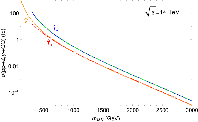
Figure 6: Production cross sections for quirks as a function of the relevant vector-like mass at a 14 TeV proton collider for $\delta_{m}=0.1$. The production of $\widehat{T}_{+}\widehat{T}_{-}$ is given by the dotted green line, which lies nearly on top of the blue $\widehat{T}_{-}\widehat{T}_{-}$ curve.

All the fermions charged under the hidden color group have masses much above 100 GeV due to LEP bounds on charged particles. The hidden confining scale is of the order of a few GeV, so we expect them to exhibit quirky Kang:2008ea dynamics, which can give a variety of new signals at colliders Harnik:2011mv ; Farina:2017cts ; Knapen:2017kly ; Evans:2018jmd ; Li:2019wce ; Li:2020aoq . After production they are connected by a string of hidden color flux which, because there are no light hidden color states, is stable against fragmentation. The quirky pair behaves as though connected by a string with tension $\sigma\sim 3.6\widehat{\Lambda}_{\text{QCD}}^{2}$ Lucini:2004my , see also Teper:2009uf .

Much of the subsequent dynamics can be treated semi-classically. Since these quirks carry electric charge the oscillating particles radiate soft-photons, quickly shedding energy until they reach their ground state Burdman:2008ek ; Harnik:2008ax . Annihilation is strongly suppressed in states with nonzero orbital angular momentum, so in nearly every case the quirks do not annihilate until they reach the ground state. Since the quirks are accelerated by the string tension, we can estimate their acceleration as $a=\sigma/m_{f}$. Then, using the Larmor formula we can estimate the radiated power as

$$\mathcal{P}=\frac{8\pi\alpha}{3}a^{2}=\frac{8\pi\alpha\sigma^{2}}{3m_{f}^{2}},$$ (49)

where $\alpha=e^{2}/(4\pi)$. The time it takes the quirky bound state to drop to its ground state is given by $K/\mathcal{P}$, where $K$ is the kinetic energy of the quirks. Taking $K\sim m_{f}$ we can then estimate the de-excitation time $T_{d}$ as

$$T_{d}\sim\frac{3m_{f}^{3}}{8\pi\alpha\left(3.6\widehat{\Lambda}_{\text{QCD}}^{2}\right)^{2}}\sim 4\times 10^{-19}\,\text{sec}\left(\frac{m_{f}}{\text{800 GeV}}\right)^{3}\left(\frac{\text{6 GeV}}{\widehat{\Lambda}_{\text{QCD}}}\right)^{4}.$$ (50)

Clearly, the de-excitation is very fast, leading to prompt annihilation

Depending on the masses of the hidden $\widehat{b}$ quark, the $\widehat{T}_{\pm}$ could $\beta$-decay by emitting a $W$. When the mass splitting is small the de-excitation is faster and the states typically annihilate. However, if the splitting is large it is most likely that both top-like states transition to bottom-like states. These would then de-excite and annihilate in the same way, though there would be additional $W$s in the final state.

If the $\widehat{b}$ quarks are not too heavy, then $\widehat{T}_{\pm}\widehat{b}$ combinations can be produced through the $W$ boson. If these states are similar in mass so that $\beta$-decay is slow then the bound states can lead to visible signals, like $W\gamma$ resonances, with appreciable rates. This is because the electric charge of the state prevents its decay into hidden gluons. However, larger splittings allow the heavier state to decay to the lighter promptly, diluting these signals significantly.

Because the quirks are fermions there are four $s$-wave states, one singlet and three triplet. Following Cheng:2018gvu we assume that each of these states is populated equally by production, so we take the total width $\Gamma_{\rm tot}$ of the bounds state to be

$$\Gamma_{\rm tot}=\Gamma_{s}+3\Gamma_{t},$$ (51)

where $\Gamma_{s}$ and $\Gamma_{t}$ are the widths of the singlet and triplet states respectively.

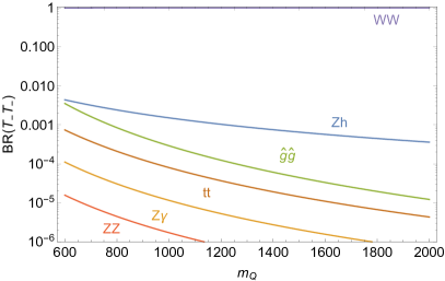
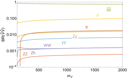
Figure 7: Branching fraction for the $s$-wave quirkonium composed of the $\widehat{T}_{-}$ (left) and $\widehat{X}$ or $\widehat{Y}$ (right) quirks. The $\widehat{T}_{-}$ quirks dominant decays are into weak gauge bosons $W^{+}W^{-}$. The dominant branching fraction for the $\widehat{X}$ and $\widehat{Y}$ is into hidden gluons.

For the $\widehat{T}_{\pm}\widehat{T}_{\pm}$ states which carry weak isospin the dominant quirkonium decays are to $WW$ with a branching fraction of about 75%. This comes from the chiral enhancement in this decay. This signal has been searched for at the LHC by both ATLAS Aaboud:2017gsl ; Aaboud:2017fgj and CMS Sirunyan:2016cao ; Sirunyan:2017acf . The next largest fractions are into $Zh$, at the 10% level, which can be compared to ATLAS Aaboud:2017cxo and CMS Khachatryan:2016cfx ; Sirunyan:2018fuh searches. All other visible final states are suppressed well below the percent level, see Fig. 7. Of these, the most likely LHC signal is a new scalar resonance decaying to $WW$, though this does depend on the $\widehat{b}$-quirk mass. As shown in Fig. 8, current searches are not yet sensitive to these signals. Here we assume a production of the $\widehat{T}_{-}\widehat{T}_{-}$ directly, and through production of the $\widehat{T}_{+}$ state which then decays to a soft $Z$ and $\widehat{T}_{-}$. While the LHC is not yet sensitive to these signals, the high luminosity run (dashed red line) will probe the most natural regions of parameter space ATL-PHYS-PUB-2018-022 .

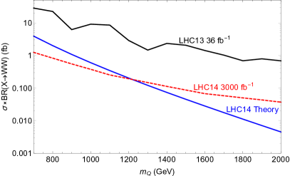
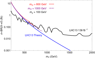
Figure 8: Left: Comparison of LHC 13 reach in $W^{+}W^{-}$ resonance searches for a $\widehat{T}_{-}\widehat{T}_{-}$ bound state (black) to the theoretical 14 TeV prediction (blue) and expected sensitivity of the high luminosity run (dashed red). Right: Comparison of LHC 13 reach in dilepton resonance searches for $\widehat{X}\widehat{X}$ and $\widehat{Y}\widehat{Y}$ bound states (black) to the theoretical 13 TeV prediction (blue). Contributions from $\widehat{T}$ states included for $m_{Q}=800$ (1000) GeV in red dashed (purple dash-dotted) curve for DM masses greater than 100 GeV.

The $\widehat{X}$ and $\widehat{Y}$ particles only couple to visible states through hypercharge, hence there is no rate into $Zh$ and the rate into $WW$ vanishes when the $Z$ mass can be neglected. The largest coupling is to hidden gluons, so this dominates the branching fractions. These gluons shower and hadronize into hidden QCD glueballs, some fraction which may have displaced decays at the LHC Chacko:2015fbc . However, they can also annihilate into $\bar{f}f$ and EW gauge bosons through their hypercharge coupling, see Fig. 7. Of these, dilepton and diphoton channels have the greatest discovery potential because the signal is so clean, which has motivated searches at both ATLAS Aaboud:2017yyg ; Aad:2019fac and CMS Sirunyan:2018wnk ; CMS:2019tbu . In the right panel of Fig. 8 we compare the reach of the ATLAS search Aad:2019fac to the theoretical prediction. We see that quirks below about 550 GeV are in tension with current collider bounds. Seeing that the predicted cross section is near the experimental limit, it is likely that by the end of the LHC run 3, with 300 $\text{fb}^{-1}$, any quirks of this type below a TeV will be discovered. Further LHC runs can probe even larger $m_{\widehat{V}}$, but we note that taking this mass larger does not affect the naturalness of the Higgs mass. It does, however, indicate that the DM is heavier, see Eq. (27).

When $m_{V}>m_{-}+m_{\chi}$ the $\widehat{X},\widehat{Y}$ quirks will quickly decay, $\widehat{V}\to\widehat{T}_{-}+\chi$. In this case the powerful dilepton resonance search will not apply. Instead, the production cross section for $T_{-}$ bound states must include this, in general small, additional mode. A similar story holds if $m_{-}>m_{V}+m_{\chi}$, where now the $\widehat{T}_{-}$ quirk decays promptly to an $\widehat{X}$ or $\widehat{Y}$ and a DM scalar. Then, the dilepton bounds would apply to the $\widehat{T}$ production. For lighter $m_{Q}$ this can strengthen the bound on $m_{V}$. The red dashed and purple dash-dotted lines on the dilepton bound in Fig. 8 correspond to taking $m_{Q}=800$ GeV and $m_{Q}=1000$ GeV, respectively, and the DM mass of 100 GeV. By taking the DM heavier these lines would cut off earlier, at $m_{V}=m_{\pm}-m_{\chi}$.

In summary, standard collider searches for prompt visible objects do constrain $m_{\widehat{V}}>550$ GeV, but the other parameters of the model are less restricted. However, both the displaced searches related to the hidden sector glueballs and dilepton and diboson resonance searches can provide evidence for the hidden QCD sector at the LHC. As we shall see in the next section, this parametric freedom can lead to viable DM, and complementary search strategies from DM experiments.

4 Dark matter phenomenology

In this section we detail the phenomenology of the DM candidate $\chi$, the complex scalar charge under the global symmetry $U(1)_{D}$. As mentioned above, this global symmetry stabilizes the DM. All the SM fields and the quirky top partners $\widehat{T}_{\pm}$ are $U(1)_{D}$ neutral, whereas the quirky fermions $\widehat{X}$ and $\widehat{Y}$ are charged. The $U(1)_{D}$ global symmetry is exact, so we can associate a discrete dark $\mathbb{Z}_{2}$ parity under which,

$$\chi\overset{\mathbb{Z}_{2}}{\to}-\chi,\qquad\widehat{X}\overset{\mathbb{Z}_{2}}{\to}-\widehat{X},\qquad\widehat{Y}\overset{\mathbb{Z}_{2}}{\to}-\widehat{Y},$$ (52)

but more generally we simply consider particles in this sector as carrying a global dark charge, which prevents their decay. Since the quirky states $\widehat{X}$ and $\widehat{Y}$ have the fractional SM electric charge $2/3$ they cannot be the DM. However, the SM neutral complex scalar $\chi$ is our DM candidate as long as it is the lightest $U(1)_{D}$ charged particle.

To determine the success of this scalar as explaining the observed DM in the universe, in what follows we calculate the relic abundance and DM-nucleon cross section for the direct detection in our model. We then consider the dark matter annihilation for the indirect detection and impose the collider constraints on our parameter space. We find that much of the natural parameter space of this model has not yet been conclusively probed by experiment, but is expected to be covered next several years.

4.1 Relic abundance

The thermal relic density of the scalar $\chi$ is obtained using the standard freeze-out analysis. Figures 9 and 10 show the relevant Feynman diagrams for the DM annihilation and semi-annihilation/conversion, respectively. The Boltzmann equation for the DM annihilation and semi-annihilation/conversion processes is

$$\frac{dn_{\chi}}{dt}= -3{\cal H}n_{\chi}-\langle\sigma^{\chi\chi\phi\phi^{\prime}}_{v_{\text{M\o l}}}\rangle\Big{(}n_{\chi}^{2}-\bar{n}_{\chi}^{2}\Big{)}$$

$$-\langle\sigma^{X\widehat{V}\widehat{T}_{\!\pm}\phi}_{v_{\text{M\o l}}}\rangle\Big{(}n_{\chi}n_{\widehat{V}}-\bar{n}_{\chi}\bar{n}_{\widehat{V}}\frac{n_{\widehat{T}_{\!\pm}}}{\bar{n}_{\widehat{T}_{\!\pm}}}\Big{)}-\langle\sigma^{\chi\widehat{T}_{\!\pm}\widehat{V}\phi}_{v_{\text{M\o l}}}\rangle\Big{(}n_{\chi}n_{\widehat{T}_{\!\pm}}-\bar{n}_{\chi}\bar{n}_{\widehat{T}_{\!\pm}}\frac{n_{\widehat{V}}}{\bar{n}_{\widehat{V}}}\Big{)}$$

$$-\langle\sigma^{\chi\chi\widehat{T}_{\!\pm}\widehat{T}_{\!\pm}}_{v_{\text{M\o l}}}\rangle\Big{(}n_{\chi}^{2}-\bar{n}_{\chi}^{2}\frac{n_{\widehat{T}_{\!\pm}}^{2}}{\bar{n}_{\widehat{T}_{\!\pm}}^{2}}\Big{)}-\langle\sigma^{\chi\chi\widehat{V}\widehat{V}}_{v_{\text{M\o l}}}\rangle\Big{(}n_{\chi}^{2}-\bar{n}_{\chi}^{2}\frac{n_{\widehat{V}}^{2}}{\bar{n}_{\widehat{V}}^{2}}\Big{)},$$ (53)

where $\phi(\phi^{\prime})$ are the SM fields: $h,t,W,Z,\gamma,\cdots$. Also, ${\cal H}$ is the Hubble parameter and $n_{i}$ is the number density of species $i$, whereas the $\bar{n}_{i}$ is its thermal equilibrium value. The quantity $\langle\sigma^{ijkl}_{v_{\text{M\o l}}}\rangle\!\equiv\!\langle\sigma(ij\to kl)\,{v_{\text{M\o l}}}\rangle$ is the thermal averaged cross-section of the initial states $ij$ to final states $kl$ with $v_{\text{M\o l}}$ being the Møller velocity. The last term in the first line of Eq. (53) describes the dynamics of the standard DM annihilation to the SM final states as shown in Fig. 9. The second and third lines describe the semi-annihilation and conversion processes shown in Fig. 10.

Figure 9: The Feynman diagrams for the DM annihilation to SM.

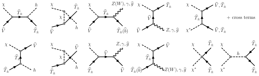
Figure 10: The Feynman diagrams for the DM semi-annihilation/conversion through the dark quirks.

The dominant DM annihilation channels are to the SM, i.e. $\chi\chi^{\ast}\to WW,hh,ZZ,t\bar{t},b\bar{b}$, while the semi-annihilation and conversion processes are only relevant if the masses the quirk states ($\widehat{V},\widehat{T}_{\pm}$) are similar to $m_{\chi}$. When the quirk masses are much larger than the DM, their thermal distributions are Boltzmann suppressed, making semi-annihilation or conversion processes very rare as compared to the standard annihilation processes. The relevant Feynman rules to calculate the DM annihilation or semi-annihilation processes are given in Appendix B. The DM relic abundance is computed using the public code micrOMEGAs Belanger:2018mqt .

Before discussing these results we emphasis some of the features of this model.

• The top partners are SM color neutral, therefore the symmetry breaking scale $f$ may be at or below a TeV. This leads to significant improvements in the fine-tuning while simultaneously allowing a larger window for the pNGB DM masses in comparison to colored top partner models Balkin:2017aep ; Frigerio:2012uc ; DaRold:2019ccj .

• The DM annihilations to SM are dominated by $s$-channel Higgs exchange. The amplitude for such processes is,

  $${\cal M}_{\chi\chi\phi\phi^{\prime}}\propto\Big{(}\frac{s}{f^{2}}-2\lambda_{h\chi}\Big{)}v,$$ (54)

  where $s\!=\!4m_{\chi}^{2}$. The $s$ dependent term originates from the derivative coupling $\partial_{\mu}h\,\partial_{\mu}(\chi^{\ast}\chi)$, while the $\lambda_{h\chi}$ term is a loop induced explicit breaking of the $\chi$ shift symmetry, see Eq. (19).

• When the standard DM annihilation processes dominate (which we see below is typically the case), the DM relic abundance can be estimated as,

  $$\Omega_{\chi}h^{2}\approx 0.12\left(\frac{2.2\!\times\!10^{-26}\,{\rm cm}^{3}{\rm s}^{-1}}{\langle\sigma(\chi\chi^{\ast}\to{\rm SM})v_{\text{M\o l}}\rangle}\right),$$ (55)

  where $0.12$ is the observed DM relic abundance by the PLANCK satellite Aghanim:2018eyx .

• The thermal averaged annihilation cross section to SM fields via $s$-channel Higgs exchange is proportional to

  $$\langle\sigma(\chi\chi^{\ast}\to{\rm SM})v_{\text{M\o l}}\rangle\propto\frac{1}{m_{\chi}^{2}}\Big{(}\frac{4m_{\chi}^{2}}{f^{2}}-2\lambda_{h\chi}c_{v}^{2}\Big{)}^{2},$$ (56)

  which implies that in the limit $\lambda_{h\chi}\to 0$, i.e. no explicit shift symmetry breaking, the cross section is proportional to $m_{\chi}^{2}/f^{4}$. Hence, for a given $m_{\chi}$ the relic abundance, $\Omega_{\chi}h^{2}$, scales as $f^{4}$.

• For $m_{\chi}^{2}/f^{2}\ll 1$, $\chi$ annihilation proceeds through the portal coupling $\lambda_{h\chi}$. When $m_{\chi}^{2}\sim\lambda_{h\chi}f^{2}/2$ the annihilation cross-section drops due to cancellation between the $s$-channel process, enhancing the relic abundance. For $m_{\chi}^{2}\gg\lambda_{h\chi}f^{2}/2$ the DM relic abundance falls like $1/m_{\chi}^{2}$ for fixed $f$.

In Fig. 11, we show the relic abundance $\Omega_{\chi}h^{2}$ for two benchmark values of $\lambda_{h\chi}\!=\!0.005$ and $0.025$ as a function of $m_{\chi}$ with fixed $f\!/\!v\!=\!4,6,8,10$. Notice that for masses below $50\;\hbox{GeV}$ the DM tends to be overproduced. This is because the thermal averaged cross-section in this region is directly proportional to the portal coupling $\lambda_{h\chi}$, which direct detection constrains to be relatively small (see below). On the other hand, for $m_{\chi}\!\sim\!m_{h}/2$ the relic abundance drops sharply due to the resonant enhancement of the Higgs portal cross-section. For DM masses $m_{\chi}^{2}\sim\lambda_{h\chi}f^{2}/2$ there is cancelation in the cross-section as a result the relic abundance enhances which produces the peaks in Fig. 11. For larger DM masses the cross section is proportional to $m_{\chi}^{2}/f^{4}$ and the relic density drops as DM mass increases.

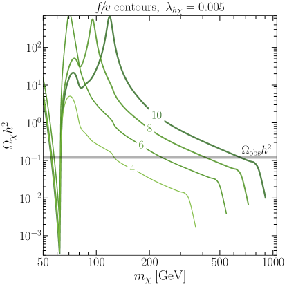
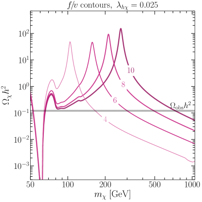
Figure 11: The left (right) plot shows the DM relic abundance $\Omega_{\chi}h^{2}$ as a function of DM mass $m_{\chi}$ for $\lambda_{h\chi}\!=\!0.005\,(0.025)$ with values of $f\!/\!v\!=\!4,6,8,10$. The gray line indicates observed relic abundance $\Omega_{\rm obs}h^{2}\!=\!0.12$.

For the case $\lambda_{h\chi}\!=\!0.005$ (left-panel), the relic density curves terminate when the DM becomes heavier than the quirk states $\widehat{X},\widehat{Y}$. These states are bound by the dark color force into quirky bound states, which then efficiently annihilate due to their electric charge, making them an unsuitable thermal DM candidate. There is also a sharp drop in the relic density at the end of each curve, which is due to an $s$-channel resonant enhancement of semi-annihilation processes, i.e. $\chi\widehat{V}\to\widehat{T}_{\pm}\to\widehat{T}_{\pm}{\rm SM}$, as shown in Fig. 10. The semi-annihilation processes are only significant when $m_{\chi}\approx m_{V}\approx m_{\pm}/2$ and in most of the parameter space are inefficient as compared to the standard annihilation processes. Since the portal coupling $\lambda_{h\chi}$ is proportional to $r_{Q}=m_{V}^{2}/m_{Q}^{2}$ it can be reduced for relatively light vector-like quirks $\widehat{V}$. However, collider searches at the LEP and LHC put a lower bound these vector-like quirks, see Sec. 3.3.

We see that the smallest mass that produces the correct DM thermal relic is near the Higgs resonance region, above $\sim\!50\;\hbox{GeV}$. This is fairly independent of $f\!/\!v$ and $\lambda_{h\chi}$. However, the largest DM masses which leads to correct relic abundance does depend on $f\!/\!v$ and $\lambda_{h\chi}$. Since naturalness prefers a smaller $f\!/\!v$ and $\lambda_{h\chi}$ is constrained by direct detection (see below), we find that restricting $f\!/\!v\!\leq\!10$ puts an upper bound of $m_{\chi}\lesssim 1\;\hbox{TeV}$ for obtaining the correct relic.

4.2 Direct detection

The WIMP DM scenario is being thoroughly tested by direct detection experiments. We here highlight the main features of our pNGB DM construction where direction detection null results are explained naturally.

At tree-level the DM-nucleon interaction is only mediated by $t$-channel Higgs exchange. As discussed above, the DM-Higgs interaction has two sources: (i) the derivative coupling $\sim\!(\partial_{\mu}h)\partial_{\mu}(\chi^{\ast}\chi)/f^{2}$, and (ii) the portal coupling $\sim\!\lambda_{h\chi}h\chi^{\ast}\chi$. The strength of the derivative interaction in a $t$-channel process is suppressed by the DM momentum transferred, $t/f^{2}\!\sim\!(100\;\hbox{MeV})^{2}/f^{2}\ll 1$. For all practical purposes we can neglect such interactions. Hence the only relevant interaction for direct detection is the portal coupling $\lambda_{h\chi}$. In this case, the spin-independent DM-nucleon scattering cross-section $\sigma_{\chi N}^{\rm SI}$ can be approximated as (see e.g. Frigerio:2012uc ; Balkin:2017aep ),

$$\sigma_{\chi N}^{\rm SI}\simeq\frac{f_{N}^{2}m_{N}^{4}}{\pi m_{h}^{4}}\frac{\lambda_{h\chi}^{2}}{m_{\chi}^{2}}\approx 2.5\!\times\!10^{-46}\,{\rm cm}^{2}\left(\frac{\lambda_{h\chi}}{0.025}\right)^{2}\left(\frac{300\;\hbox{GeV}}{m_{\chi}}\right)^{2},$$ (57)

where $m_{N}$ is the nucleon mass and $f_{N}\simeq 0.3$ encapsulates the Higgs-nucleon coupling. The current bound on the spin-independent DM-nucleon cross-section for mass range $\sim\![50,\,1000]$ GeV is by XENON1T with one ton-year of exposure time Aprile:2018dbl . For instance, the upper limit on the spin-independent DM-nucleon cross-section for DM mass $300\;\hbox{GeV}$ is $\sim\!2.5\!\times\!10^{-46}$ at $90\%$ C.L. From Eq. (57) it is clear that the $\sigma_{\chi N}^{\rm SI}$ is directly proportional to the square of the portal coupling $\lambda_{h\chi}^{2}$ and inversely proportional to the square of DM mass $m_{\chi}^{2}$. Hence to satisfy the direct detection constraints we either need to reduce the portal coupling $\lambda_{h\chi}$ or increase the DM mass.

One feature of this minimal model is that $\lambda_{h\chi}$ is determined by a small number of low-energy parameters: the vector-like masses of the quirks, $m_{V}$ and $m_{Q}$. However, as noted above in Eq. (35), the top partners quirk mass $m_{Q}\!=\!c_{v}\lambda_{t}f$ is fixed in terms of $f$ to obtain the correct Higgs mass. Hence, the free parameters are $m_{\chi},f$, and $r_{Q}\!\equiv\!m_{V}^{2}/m_{Q}^{2}$. As discussed above, one can specify $f$ by requiring the correct DM relic abundance and $r_{Q}$ can be exchanged with $\lambda_{h\chi}$, which is constrained by direct detection.

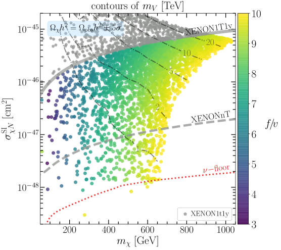
Figure 12: The DM-nucleon cross section as a function of DM mass $m_{\chi}$ with all points producing the observed relic abundance $\Omega_{\rm obs}h^{2}\!=\!0.12\pm 0.0012$. The gray points above gray curve are excluded by current XENON1T bounds, whereas the colored points (corresponding to particular $f\!/\!v$ values) are allowed.

In Fig. 12 we show the spin-independent DM-nucleon cross section $\sigma_{\chi N}^{\rm SI}$ as a function of DM mass $m_{\chi}$. We have performed a random scan of the parameter space for $f\!/\!v\!\in\![3,10]$ and $m_{V}\!\in\![m_{\chi},4\pi f]$. The lower value of the $f\!/\!v\!=\!3$ choice is enforced by the SM Higgs coupling measurement and electroweak measurements data, while the upper value of $f\!/\!v\!=\!10$ limits the tuning to $\sim$1%. The lower value of $m_{V}$ makes sure that $\chi$ is the lightest state charged under $U(1)_{D}$. All the points shown in the plot correspond to the correct relic abundance $\Omega_{\chi}h^{2}\!=\!\Omega_{\rm obs}h^{2}\!\pm 5\sigma$, where $\Omega_{\rm obs}h^{2}\!=\!0.12\pm 0.0012$ is the observed DM relic density as measured by the Planck satellite Aghanim:2018eyx . The gray (pentagon) points above the gray line are excluded by the XENON1T Aprile:2018dbl . All the colored points (color barcoded with $f\!/\!v$) are allowed by the current XENON1T constraint. The dashed gray line indicates the expected XENONnT bound Aprile:2018dbl which covers much of the more natural parameter space. However, there are points allowed below this bound above the so-called neutrino-floor (red dotted), which could be discovered by next generation detectors, e.g. LZ Akerib:2018dfk and DARWIN Aalbers:2016jon .

4.3 Indirect detection

We now turn to indirect detection. There are a variety of experiments searching for DM annihilations in the Milky Way galaxy and nearby dwarf galaxies, which are assumed to be dominated by DM. The typical signals of DM annihilation to the SM particles leads to gamma-rays, gamma-lines, and an excess of secondary products like antipositrons and antiprotons in cosmic-rays (CR). In particular, the experimental data can be used to put upper bounds on the various annihilation channels, including $WW,ZZ,hh,t\bar{t},b\bar{b},\tau^{+}\tau^{-},\cdots$. In our model the DM dominantly annihilates into $WW,hh,ZZ,t\bar{t}$ final states. We calculate the present day DM thermal averaged annihilation to the SM particles by using micrOMEGAs Belanger:2018mqt . We find that the DM thermal annihilation cross-section is $\langle\sigma v\rangle\approx 2.2\times 10^{-26}\,\mathrm{cm^{3}/s}$ for parameter values that produce the correct relic abundance. The fraction of annihilation cross-section to $W^{+}W^{-}$ is $\sim\!45\%$ and $hh/ZZ\sim\!25\%$ for $m_{\chi}\!\gtrsim\!m_{h}$. Whereas the branching fraction is dominantly into $W^{+}W^{-}$ for $m_{\chi}\in[m_{W},m_{h}]$.

In Fig. 13 we show the DM annihilation cross section to $W^{+}W^{-}$, $\langle\sigma v\rangle_{WW}$, in units of $[10^{-26}~{}\mathrm{cm^{3}/s}]$ as function of $m_{\chi}$. All the data points in this figure produce correct DM relic abundance and satisfy the XENON1T direct detection constraint. Because these points have $m_{\chi}\!>\!m_{W}$, the most dominant annihilation channels are the $WW,ZZ,hh$. In the following we summarize the most sensitive indirect detection probes in the mass range of interest.

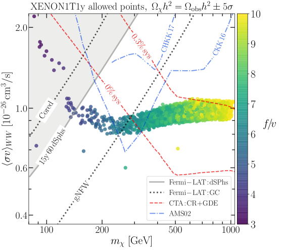
Figure 13: A parameter scan with all the points producing correct relic abundance in the $m_{\chi}$ vs $\langle\sigma v\rangle_{WW}$. Each point (color coded for different $f\!/\!v$ values) is allowed by the XENON1T1y direct detection experiment. The gray shaded region is the robust projected 95% C.L. sensitivity of Fermi-LAT with 15 years data and 60 dSphs. The dashed curves represents the CTA projected 95% C.L. sensitivity with background only (0% systematics) and 0.3% systematics, whereas the dotted and dash-dotted curves are relatively less robust 95% C.L. upper bounds due to Fermi-LAT and AMS-02, respectively.

Gamma-rays:

The most robust indirect detection bounds are due to Fermi-LAT Ackermann:2015zua and Fermi-LAT+DES Fermi-LAT:2016uux with six years of data from 15 and 45 DM dominated dwarf spheroidal galaxies (dSphs), respectively. Theses constraints are considered robust because the uncertainties associated with propagation of gamma rays are relatively small. The Fermi-LAT results Ackermann:2015zua provide upper-limits on the DM thermal annihilation cross section into several SM final states including $WW,b\bar{b},\tau^{+}\tau^{-}$, whereas, the updated analysis Fermi-LAT+DES Fermi-LAT:2016uux only includes the $b\bar{b}$ and $\tau^{+}\tau^{-}$ channels. These bounds do not constraint any of the parameter space allowed by the direct detection. However, Fermi-LAT has provided expected 95% C.L. upper-limits for the DM thermal annihilation into $b\bar{b}$ and $\tau^{+}\tau^{-}$ channels with 15 years of data and 60 dSPhs Charles:2016pgz . One can interpolate the projected upper-limit from the $\langle\sigma v\rangle_{b\bar{b}}$ to $\langle\sigma v\rangle_{WW}$ by a simple rescaling $\langle\sigma v\rangle_{WW}\simeq 1.33\langle\sigma v\rangle_{b\bar{b}}$ in the DM mass range of our interest. In Fig. 13 we show the projected 95% C.L. sensitivity on $\langle\sigma v\rangle_{WW}$ by Fermi-LAT with 15 years and 60 dSPhs by the solid (gray) curve. This sensitivity sets a lower-limit on the DM mass $m_{\chi}\gtrsim 150\;\hbox{GeV}$.

A very recent analysis Abazajian:2020tww of Fermi-LAT observations of the Galactic Center (GC) has led to stringent constraints on WIMP DM mass up to $\sim\!300\;\hbox{GeV}$. In Fig. 13 we show 95% C.L. upper bound on $\langle\sigma v\rangle_{WW}$ as dotted (black) curves due to two DM profiles: a generalized NFW (gNFW) profile and a cored profile that smoothly matches on to a NFW profile while conserving mass. The upper limit on the thermal annihilation for each DM profile in Fig. 13 is least constraining when variations of the DM profiles and the systematic uncertainties associated with different Galactic Diffuse Emission (GDE) templets are taken into account, see Abazajian:2020tww for further technical details. The Fermi-LAT GC 95% C.L. upper limit with a gNFW profile excludes our DM up to masses $\sim\!300\;\hbox{GeV}$. Assuming a cored profile, however, weakens the bound to $m_{\chi}\gtrsim 100\;\hbox{GeV}$. While the GC constraints are highly sensitive to the DM profiles and the GDE templets, they still provide an important complimentary DM probe, and with more data these uncertainties will be reduced.

Cosmic-rays:

The flux of antipositrons and antiprotons in the cosmic-rays (CR) provides another indirect probe of DM annihilation in the Galaxy. In particular recent precise AMS-02 CR antiproton flux data Aguilar:2016kjl has led to strong constraints on the DM thermal annihilation. In Refs. Cuoco:2016eej ; Cui:2016ppb the AMS-02 antiproton flux data was used to put stringent constraints on DM with masses in range $[150,1000]\;\hbox{GeV}$, see also Arina:2019tib for a recent global fit analysis of pNGB DM. The AMS-02 95% C.L. exclusion constraint on $\langle\sigma v\rangle_{WW}$ as obtained by CKK Cuoco:2016eej is shown in Fig. 13 as dash-dotted (blue) curve. This constraint excludes most of the data points between DM masses $m_{\chi}\in[225,375]\;\hbox{GeV}$. However, these constraint has large systematic uncertainties, mainly due to CR propagation and diffusion parameters Cuoco:2016eej . The updated analysis by (CHKK) Cuoco:2017iax reveals a weaker constraint in the $W^{+}W^{-}$ channel, which is also given by a dash-dotted (blue) curve. Even though the updated AMS-02 analysis does not constrain our model, future AMS CR antiproton data are likely to. Another future CR experiment is the Cherenkov Telescope Array (CTA) which is expected to be sensitive to large DM masses CTA:2018 . In Fig. 13 we show the projected sensitivity of CTA for DM annihilation to $W^{+}W^{-}$ with GDE Gamma model of Ref. Gaggero:2017jts , as a dashed (red) curve, for two assumptions of systematic error. The most optimistic implies that CTA will probe DM masses above $\sim\!300\;\hbox{GeV}$, though this is quickly weakened when systematic errors are included.

5 Conclusion

We have outlined a framework in which the Higgs and a scalar DM candidate arise pNGBs of a broken global symmetry. Because the symmetry partners of the top quark do not carry SM color, the induced scalar potential between the Higgs and the DM, which is UV insensitive, allows for improved fine-tuning and simultaneously explains null results for WIMP DM searches. The quantitative success of this framework is summarized by Fig. 14 in the $m_{\chi}$ vs $\lambda_{h\chi}$ plane with the color of scanned points corresponding to values of $f\!/\!v\in[3,10]$. This corresponds to fine-tuning in the model of about 10% to 1%, respectively.

The phenomenology can be specified by the DM mass $m_{\chi}$, the global symmetry breaking scale $f$, and the vector-like mass $m_{V}$ of the quirky fermions, which is the source of breaking the $\chi$ shift symmetry. As shown in Sec. 2.3 we can trade $m_{V}$ for $\lambda_{h\chi}$. Hence, the three free parameters of the model are $m_{\chi},f\!/\!v$, and $\lambda_{h\chi}$.

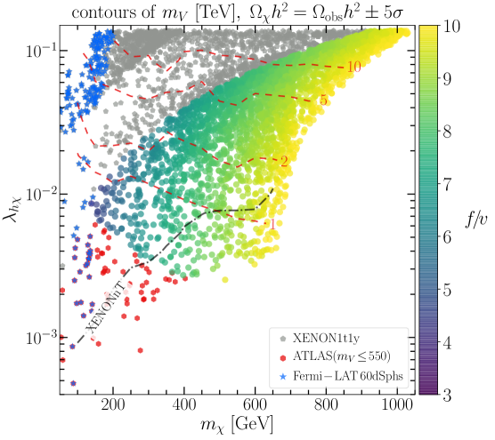
Figure 14: A parameter scan with all points producing the correct relic abundance in the $m_{\chi}$ vs $\lambda_{h\chi}$. The colored (gray hexagon) points allowed (excluded) by the XENON1T1y direct detection experiment. The allowed points are color coded for different $f\!/\!v$ values. The red (pentagon) points are excluded by the ATLAS search of quirky states with $m_{V}\lesssim 550\;\hbox{GeV}$, while the indirect detection projected 95% C.L. sensitive points due to Fermi-LAT with 15 years and 60 dSPhs are marked as blue (stars). The dashed (red) contours represent different values of $m_{V}$ [TeV], whereas the dash-dotted (black) curve gives the projected sensitivity of XENONnT.

The points in Fig. 14 scan in $m_{\chi}\!\sim\![50,1000]\;\hbox{GeV}$ and $\lambda_{h\chi}\!\sim\![0.2,0.0005]$ while required to produce the correct relic abundance $\Omega_{\chi}h^{2}=0.12\pm 5(0.012)$. The gray (pentagon) points are excluded at 90% C.L. by the direct detection experiment XENON1T with one year exposure time Aprile:2018dbl . Future direct detection XENONnT 90% C.L. reach is overlaid as the dash-dotted (black) curve, which would cover much of the allowed parameter space. Next generation experiments that will descend toward the neutrino floor will fully explore this framework.

The next most stringent constraint is due to the LHC bound on the vector-like mass $m_{V}\gtrsim 550\;\hbox{GeV}$ of the quirky fermions $\widehat{X},\widehat{Y}$ as shown in Fig. 8. This limit from the ATLAS collaboration search for dilepton resonances with $\mathrm{139~{}fb^{-1}}$ data is due to the annihilation of quirks $\widehat{V}\widehat{V}$ to $\ell^{+}\ell^{-}$. We show the bound in Fig. 14 as red (hexagon) points. Since the portal coupling $\lambda_{h\chi}$ is proportional to $m_{V}^{2}$, the lower-bound on $m_{V}$ translates to a DM mass and $f\!/\!v$ dependent lower-bound on $\lambda_{h\chi}$. We have also shown dashed (red) contours of $m_{V}=1\;\hbox{TeV}$ to $10\;\hbox{TeV}$ which shows how future LHC runs may be able to discover quirks in much of the natural parameter space. The complementarity between collider and direct detection could lead to both discovery and confirmation of this construction in the coming years, or its exclusion.

In Fig. 14 we also show how indirect detection gamma-rays 95% C.L. constraints from the Fermi-LAT 15 years with 60 dSphs as blue (star) points. This puts a lower limit on the DM mass $m_{\chi}\gtrsim 150\;\hbox{GeV}$. We have not shown in this plot the indirect detection constraints from the cosmic-rays experiments AMS-02 because of their large systematic uncertainties. However, in the future such uncertainties may be reduced, allowing experiments like AMS and CTA) to provide another complementary probe, and hopefully discovery, of this model.

In summary, this framework of WIMP dark addresses the hierarchy problem without colored symmetry partners, and consequently is only tuned at the 10% level while agreeing with all experimental bounds. However, existing experiments will soon be able to discover or exclude these more natural realizations of the model. After the searches of the HL-LHC run and next generation direct detection experiments models with fine tuning at or better than 1% may be thoroughly probed.

Appendix A $SO(7)$ Generators

In this appendix we collect all the relevant details. The $SO(7)$ generators in the fundamental representation can be written as,

$$T_{ij}^{a_{L,R}} =-\frac{i}{2}\left[\frac{1}{2}\epsilon^{abc}\left(\delta_{i}^{b}\delta_{j}^{c}-\delta_{j}^{b}\delta_{i}^{c}\right)\pm\left(\delta_{i}^{a}\delta_{j}^{4}-\delta_{j}^{a}\delta_{i}^{4}\right)\right], a_{L,R} =1,2,3,$$ (58)

$$T_{ij}^{ab} =-\frac{i}{\sqrt{2}}\left(\delta_{i}^{a}\delta_{j}^{b}-\delta_{j}^{a}\delta_{i}^{b}\right),\quad b=5,6;~{}a =1,\ldots,b-1,$$ (59)

$$T_{ij}^{\hat{a}} =-\frac{i}{\sqrt{2}}\left(\delta_{i}^{\hat{a}}\delta_{j}^{7}-\delta_{j}^{\hat{a}}\delta_{i}^{7}\right), \hat{a} =1,\ldots,6,$$ (60)

where $i,j\!=\!1,\ldots,7$. We have chosen the normalization $\text{Tr}\left[T^{a}T^{b}\right]=\delta^{ab}$. The unbroken generators $T_{ij}^{a_{L,R}},T_{ij}^{ab}$ correspond to the $SO(6)$, whereas the broken generators $T_{ij}^{\hat{a}}$ correspond to the $SO(7)/SO(6)$ coset. Note that $T_{ij}^{a_{L,R}}$ correspond to the custodial $SO(4)_{C}\cong SU(2)_{L}\times SU(2)_{R}$ subgroup of $SO(6)$.

Appendix B Feynman rules and Quirk Processes

Table 1: Some of the most relevant Feynman rules of our model are listed in this table, see the text for the corresponding notation.

In this appendix we record formulae for quirk production and decay widths. The relevant Feynman rules are given in Table 1. The decays are typically similar to the results Barger:1987xg ; Fok:2011yc , using the methods outlined in Kuhn:1979bb ; Guberina:1980dc . The couplings of the $Z$ to fermions are taken to be

$$\frac{g}{2c_{W}}\gamma^{\mu}(v_{i}-a_{i}\gamma_{5}),$$ (61)

where $c_{W}\equiv\cos\theta_{W}$. For convenience we define the following

$$R_{i}=\frac{m_{i}^{2}}{M^{2}},\ \ \ \ \beta_{ij}=\sqrt{1-2(R_{i}+R_{j})+(R_{i}-R_{j})^{2}},$$ (62)

where $M$ is the mass of the relevant bound state. The number of colors in the quirk confining group is $N_{\widehat{c}}$.

We calculate the cross section $pp\to Z,\gamma\to\overline{f}f$ from the quark $q$ initiated partonic cross section $\tilde{\sigma}$ into a quirk $Q$ pair by

$$\sigma(pp\to QQ)(s)=\sum_{q}\int_{\frac{4m_{Q}^{2}}{s}}d\tau L_{\overline{q}q}\tilde{\sigma}(\overline{q}q\to\overline{Q}Q)(\tilde{s}=\tau s),$$ (63)

where

$$L_{\overline{q}q}(\tau)=\int^{1}_{\tau}\frac{dx}{x}\left[f_{q}(x)f_{\overline{q}}\left(\frac{\tau}{x}\right)+f_{q}\left(\frac{\tau}{x}\right)f_{\overline{q}}(x)\right],$$ (64)

is defined in terms of the MSTW2008 PDFs Martin:2009iq $f_{q}(x)$, we take the factorization scale to be $\sqrt{\tilde{s}}/2$.

Because the quirk states decays from all $\ell>0$ states are strongly suppressed Kang:2008ea we only consider decays of the singlet ${}^{1}\!S_{0}$ and triplet ${}^{3}\!S_{1}$ states. Each of these decay widths depends on the radial wavefunction $R(0)$ of the quirk bound state. This factor is nonperturbative and not exactly known, so we simply give each decay width in units of the unknown factor $\left|R(0)\right|^{2}$.

The neutral states are composed of fermionic quirks $Q$ with mass $m_{Q}$. In this case the $Z$ couplings are labeled $v_{Q}$ and $a_{Q}$, and the electric charge is denoted $Q_{Q}$. The mass is denoted $m_{Q}$ and we take the meson mass to be $M$, which for heavy constituents is approximately $2m_{Q}$.

We begin with decays to fermion pairs. These fermions have $Z$ couplings $v_{f}$ and $a_{f}$ as well as electric charge $Q_{f}$. They also come in $N_{c}$ colors. The decays to $\overline{f}f$ are,

$$\Gamma({}^{1}\!S_{0}\to\overline{f}f)= \frac{2N_{\widehat{c}}N_{c}\alpha_{W}^{2}a_{f}^{2}a_{Q}^{2}m_{f}^{2}m_{Q}^{2}}{c_{W}^{4}m_{Z}^{4}M^{2}}\beta_{ff},$$ (65)

$$\Gamma({}^{3}\!S_{1}\to\overline{f}f)= \frac{N_{\widehat{c}}N_{c}\alpha_{W}^{2}}{12M^{2}}\beta_{ff}\left[(1+2R_{f})\left(4s_{W}^{2}Q_{Q}Q_{f}+\frac{v_{Q}v_{f}}{c_{W}^{2}(1-R_{Z})}\right)^{2}+\frac{v_{Q}^{2}a_{f}^{2}\beta_{ff}^{2}}{c_{W}^{4}(1-R_{Z})^{2}}\right],$$ (66)

where $\alpha_{W}\equiv g^{2}/(4\pi)$. Next, we turn to decays into $Z\gamma$,

$$\Gamma({}^{1}\!S_{0}\to Z\gamma)= \frac{8N_{\widehat{c}}\alpha_{W}\alpha Q_{Q}^{2}v_{Q}^{2}}{c_{W}^{2}M^{2}}(1-R_{Z}),$$ (67)

$$\Gamma({}^{3}\!S_{1}\to Z\gamma)= \frac{8N_{\widehat{c}}\alpha_{W}\alpha Q_{Q}^{2}a_{Q}^{2}m_{Q}^{2}}{3c_{W}^{2}m^{2}_{Z}M^{2}}(1-R_{Z}^{2}).$$ (68)

The decays to $ZZ$ ,

$$\Gamma({}^{1}\!S_{0}\to ZZ)= \frac{N_{\widehat{c}}\alpha_{W}^{2}(v_{Q}^{2}+a_{Q}^{2})^{2}}{4M^{2}c_{W}^{4}(1-2R_{Z})^{2}}\beta_{ZZ}^{3},$$ (69)

$$\Gamma({}^{3}\!S_{1}\to ZZ)= \frac{N_{\widehat{c}}\alpha_{W}^{2}v_{Q}^{2}a_{Q}^{2}}{3c_{W}^{2}M^{2}R_{Z}(1-2R_{Z})^{2}}\beta_{ZZ}^{5}.$$ (70)

Next, to $Zh$,

$$\Gamma({}^{1}\!S_{0}\to Zh)= \frac{N_{\widehat{c}}\alpha_{W}^{2}a_{Q}^{2}M^{2}}{16m_{Z}^{4}c_{W}^{4}}\beta_{Zh}^{3},$$ (71)

$$\Gamma({}^{3}\!S_{1}\to Zh)= \frac{N_{\widehat{c}}\alpha_{W}^{2}v_{Q}^{2}\beta_{Zh}}{12c_{W}^{2}M^{2}m_{W}^{2}}\left\{\left[2+\frac{1}{4R_{Z}}\left(1+R_{Z}-R_{h}\right)^{2}\right]\left[\frac{2m_{Q}R_{Z}}{1-R_{Z}}-\frac{v\lambda_{Q}(1+R_{Z}-R_{W}^{2})}{1-R_{Z}-R_{h}}\right]^{2}\right.$$

$$\left.+\frac{v\lambda_{Q}\beta_{Zh}^{2}(1-R_{h}+R_{Z})}{2R_{Z}(1-R_{Z}-R_{h})}\left[\frac{2m_{Q}R_{Z}}{1-R_{Z}}-\frac{v\lambda_{Q}(1+R_{Z}-R_{W}^{2})}{1-R_{Z}-R_{h}}\right]+\frac{\beta_{Zh}^{4}v^{2}\lambda^{2}_{Q}}{4R_{Z}(1-R_{Z}-R_{h})^{2}}\right\},$$ (72)

where $\lambda_{Q}$ is the Yukawa coupling of the quirks to the Higgs. Finally, to $h\gamma$,

$$\Gamma({}^{1}\!S_{0}\to h\gamma)= 0,$$ (73)

$$\Gamma({}^{3}\!S_{1}\to h\gamma)= \frac{N_{\widehat{c}}\alpha Q_{Q}^{2}\lambda^{2}_{Q}(1-R_{h})}{3\pi M^{2}}.$$ (74)

One might expect decays to scalar pairs like $hh$ and, in the case of the $\widehat{X}$ and $\widehat{Y}$ quirks, $\chi\chi^{\ast}$. However, $CP$ and angular momentum conservation forbid such decays from the $s$-wave states, though higher angular momentum states do allow these decays.

We now turn to decays into $W^{+}W^{-}$. We label the $SU(2)_{L}$ partner of $Q$ by $q$, with mass $m_{q}$ etc. The $W$ couplings $v_{W}$ and $a_{W}$ are defined by the interaction

$$\frac{g}{2\sqrt{2}}\gamma^{\mu}(v_{W}-a_{W}\gamma^{5}).$$ (75)

We note that this decay depends upon the electric charge of particle that makes up the bound state in a nontrivial way. This is due to the diagrams related to the $t$- or $u$-channel exchange of the $SU(2)_{L}$ partner of the particle making up the bound state. Mesons made by a quirk with positive charge involve a different diagram than those with negative charge. None of these subtleties affect the singlet case, but we do distinguish the triplet cases as ${}^{3}\!S_{1}^{(+,-)}$, where the superscript denotes whether the quirk has positive or negative electric charge. The decays to $W^{+}W^{-}$ are

$$\Gamma({}^{1}\!S_{0}\to W^{+}W^{-}) =\frac{N_{\widehat{c}}\alpha_{W}^{2}(v_{W}^{2}+a_{W}^{2})^{2}}{8M^{2}(1+4R_{q}-4R_{W})^{2}}\beta_{WW}^{3},$$ (76)

$$\Gamma({}^{3}\!S_{1}^{(\pm)}\to W^{+}W^{-}) =\frac{N_{\widehat{c}}\alpha_{W}^{2}\beta_{WW}^{3}}{192R_{W}^{2}M^{2}}\left\{\frac{16v_{W}^{2}a_{W}^{2}\beta_{WW}^{2}}{(1+4R_{q}-4R_{W})^{2}}-6\frac{R_{W}}{m_{Q}^{2}}\left[\frac{v_{W}^{2}(m_{Q}-m_{q})+a_{W}^{2}(m_{Q}+m_{q})}{1+4R_{q}-4R_{W}}\right]^{2}\right.$$

$$+(1+10R_{W})\left[4Q_{Q}s_{W}^{2}+\frac{2v_{Q}}{1-R_{Z}}\mp\frac{m_{q}}{m_{Q}}\frac{v_{W}^{2}-a_{W}^{2}}{1+4R_{q}-4R_{W}}\right]^{2}$$

$$\left.+2R_{W}(5+6R_{W})\left[4Q_{Q}s_{W}^{2}+\frac{2v_{Q}}{1-R_{Z}}\mp\frac{v_{W}^{2}+a_{W}^{2}}{1+4R_{q}-4R_{W}}\right]^{2}\right\}.$$ (77)

We also record the decays involving hidden gluons. These are taken from Cheung:2008ke .

$$\Gamma({}^{1}\!S_{0}\to\widehat{g}\,\widehat{g})= \frac{N_{\widehat{c}}^{2}-1}{N_{\widehat{c}}M^{2}}\widehat{\alpha}_{s}^{2},$$ (78)

$$\Gamma({}^{3}\!S_{1}\to\widehat{g}\,\widehat{g}\,\widehat{g})= \frac{(N_{\widehat{c}}^{2}-1)(N_{\widehat{c}}^{2}-4)(\pi^{2}-9)}{9\pi N_{\widehat{c}}^{2}M^{2}}\widehat{\alpha}_{s}^{3},$$ (79)

$$\Gamma({}^{3}\!S_{1}\to\gamma\widehat{g}\,\widehat{g})= \frac{4Q_{f}^{2}(N_{\widehat{c}}^{2}-1)(\pi^{2}-9)}{3\pi M^{2}N_{\widehat{c}}}\alpha\widehat{\alpha}_{s}^{2},$$ (80)

where we have denoted the hidden sector strong coupling by $\widehat{\alpha}_{s}$. Finally, the singlet state can also decay to photons

$$\Gamma({}^{1}\!S_{0}\to\gamma\gamma)=\frac{4N_{\widehat{c}}Q_{Q}^{4}}{M^{2}}\alpha^{2}.$$ (81)

References

- (1) ATLAS Collaboration, G. Aad et al., “Observation of a new particle in the search for the Standard Model Higgs boson with the ATLAS detector at the LHC,” Phys. Lett. B716 (2012) 1–29, [arXiv:1207.7214].
- (2) CMS Collaboration, S. Chatrchyan et al., “Observation of a New Boson at a Mass of 125 GeV with the CMS Experiment at the LHC,” Phys. Lett. B716 (2012) 30–61, [arXiv:1207.7235].
- (3) Z. Chacko, H.-S. Goh, and R. Harnik, “The Twin Higgs: Natural electroweak breaking from mirror symmetry,” Phys. Rev. Lett. 96 (2006) 231802, [hep-ph/0506256].
- (4) R. Barbieri, T. Gregoire, and L. J. Hall, “Mirror world at the large hadron collider,” hep-ph/0509242.
- (5) G. Burdman, Z. Chacko, H.-S. Goh, and R. Harnik, “Folded supersymmetry and the LEP paradox,” JHEP 02 (2007) 009, [hep-ph/0609152].
- (6) D. Poland and J. Thaler, “The Dark Top,” JHEP 11 (2008) 083, [arXiv:0808.1290].
- (7) H. Cai, H.-C. Cheng, and J. Terning, “A Quirky Little Higgs Model,” JHEP 05 (2009) 045, [arXiv:0812.0843].
- (8) N. Craig, S. Knapen, and P. Longhi, “Neutral Naturalness from Orbifold Higgs Models,” Phys. Rev. Lett. 114 no. 6, (2015) 061803, [arXiv:1410.6808].
- (9) N. Craig, S. Knapen, and P. Longhi, “The Orbifold Higgs,” JHEP 03 (2015) 106, [arXiv:1411.7393].
- (10) B. Batell and M. McCullough, “Neutrino Masses from Neutral Top Partners,” Phys. Rev. D92 no. 7, (2015) 073018, [arXiv:1504.04016].
- (11) J. Serra and R. Torre, “Neutral naturalness from the brother-Higgs model,” Phys. Rev. D97 no. 3, (2018) 035017, [arXiv:1709.05399].
- (12) C. Csáki, T. Ma, and J. Shu, “Trigonometric Parity for Composite Higgs Models,” Phys. Rev. Lett. 121 no. 23, (2018) 231801, [arXiv:1709.08636].
- (13) T. Cohen, N. Craig, G. F. Giudice, and M. Mccullough, “The Hyperbolic Higgs,” JHEP 05 (2018) 091, [arXiv:1803.03647].
- (14) H.-C. Cheng, L. Li, E. Salvioni, and C. B. Verhaaren, “Singlet Scalar Top Partners from Accidental Supersymmetry,” JHEP 05 (2018) 057, [arXiv:1803.03651].
- (15) B. M. Dillon, “Neutral-naturalness from a holographic composite Higgs model,” Phys. Rev. D99 no. 11, (2019) 115008, [arXiv:1806.10702].
- (16) L.-X. Xu, J.-H. Yu, and S.-H. Zhu, “Minimal Neutral Naturalness Model,” arXiv:1810.01882.
- (17) J. Serra, S. Stelzl, R. Torre, and A. Weiler, “Hypercharged Naturalness,” JHEP 10 (2019) 060, [arXiv:1905.02203].
- (18) I. Garcia Garcia, R. Lasenby, and J. March-Russell, “Twin Higgs WIMP Dark Matter,” Phys. Rev. D92 no. 5, (2015) 055034, [arXiv:1505.07109].
- (19) N. Craig and A. Katz, “The Fraternal WIMP Miracle,” JCAP 1510 no. 10, (2015) 054, [arXiv:1505.07113].
- (20) I. Garcia Garcia, R. Lasenby, and J. March-Russell, “Twin Higgs Asymmetric Dark Matter,” Phys. Rev. Lett. 115 no. 12, (2015) 121801, [arXiv:1505.07410].
- (21) M. Farina, “Asymmetric Twin Dark Matter,” JCAP 1511 no. 11, (2015) 017, [arXiv:1506.03520].
- (22) M. Freytsis, S. Knapen, D. J. Robinson, and Y. Tsai, “Gamma-rays from Dark Showers with Twin Higgs Models,” JHEP 05 (2016) 018, [arXiv:1601.07556].
- (23) M. Farina, A. Monteux, and C. S. Shin, “Twin mechanism for baryon and dark matter asymmetries,” Phys. Rev. D94 no. 3, (2016) 035017, [arXiv:1604.08211].
- (24) R. Barbieri, L. J. Hall, and K. Harigaya, “Minimal Mirror Twin Higgs,” JHEP 11 (2016) 172, [arXiv:1609.05589].
- (25) R. Barbieri, L. J. Hall, and K. Harigaya, “Effective Theory of Flavor for Minimal Mirror Twin Higgs,” JHEP 10 (2017) 015, [arXiv:1706.05548].
- (26) Y. Hochberg, E. Kuflik, and H. Murayama, “Twin Higgs model with strongly interacting massive particle dark matter,” Phys. Rev. D99 no. 1, (2019) 015005, [arXiv:1805.09345].
- (27) H.-C. Cheng, L. Li, and R. Zheng, “Coscattering/Coannihilation Dark Matter in a Fraternal Twin Higgs Model,” JHEP 09 (2018) 098, [arXiv:1805.12139].
- (28) J. Terning, C. B. Verhaaren, and K. Zora, “Composite Twin Dark Matter,” Phys. Rev. D99 no. 9, (2019) 095020, [arXiv:1902.08211].
- (29) S. Koren and R. McGehee, “Freeze-Twin Dark Matter,” arXiv:1908.03559.
- (30) M. Badziak, G. Grilli Di Cortona, and K. Harigaya, “Natural Twin Neutralino Dark Matter,” arXiv:1911.03481.
- (31) R. Balkin, M. Ruhdorfer, E. Salvioni, and A. Weiler, “Charged Composite Scalar Dark Matter,” JHEP 11 (2017) 094, [arXiv:1707.07685].
- (32) R. Balkin, M. Ruhdorfer, E. Salvioni, and A. Weiler, “Dark matter shifts away from direct detection,” JCAP 1811 no. 11, (2018) 050, [arXiv:1809.09106].
- (33) M. Frigerio, A. Pomarol, F. Riva, and A. Urbano, “Composite Scalar Dark Matter,” JHEP 07 (2012) 015, [arXiv:1204.2808].
- (34) L. Da Rold and A. N. Rossia, “The Minimal Simple Composite Higgs Model,” JHEP 12 (2019) 023, [arXiv:1904.02560].
- (35) J. Kang and M. A. Luty, “Macroscopic Strings and ‘Quirks’ at Colliders,” JHEP 11 (2009) 065, [arXiv:0805.4642].
- (36) N. Craig, A. Katz, M. Strassler, and R. Sundrum, “Naturalness in the Dark at the LHC,” JHEP 07 (2015) 105, [arXiv:1501.05310].
- (37) B. Gripaios, A. Pomarol, F. Riva, and J. Serra, “Beyond the Minimal Composite Higgs Model,” JHEP 04 (2009) 070, [arXiv:0902.1483].
- (38) S. R. Coleman and E. J. Weinberg, “Radiative Corrections as the Origin of Spontaneous Symmetry Breaking,” Phys. Rev. D7 (1973) 1888–1910.
- (39) R. Contino, D. Greco, R. Mahbubani, R. Rattazzi, and R. Torre, “Precision Tests and Fine Tuning in Twin Higgs Models,” Phys. Rev. D96 no. 9, (2017) 095036, [arXiv:1702.00797].
- (40) G. Burdman, Z. Chacko, R. Harnik, L. de Lima, and C. B. Verhaaren, “Colorless Top Partners, a 125 GeV Higgs, and the Limits on Naturalness,” Phys. Rev. D91 no. 5, (2015) 055007, [arXiv:1411.3310].
- (41) K. Fujii et al., “Physics Case for the 250 GeV Stage of the International Linear Collider,” arXiv:1710.07621.
- (42) R. Franceschini et al., “The CLIC Potential for New Physics,” arXiv:1812.02093.
- (43) FCC Collaboration, A. Abada et al., “FCC Physics Opportunities,” Eur. Phys. J. C79 no. 6, (2019) 474.
- (44) M. Cepeda et al., “Report from Working Group 2,” CERN Yellow Rep. Monogr. 7 (2019) 221–584, [arXiv:1902.00134].
- (45) J. E. Juknevich, “Pure-glue hidden valleys through the Higgs portal,” JHEP 08 (2010) 121, [arXiv:0911.5616].
- (46) Y. Chen et al., “Glueball spectrum and matrix elements on anisotropic lattices,” Phys. Rev. D73 (2006) 014516, [hep-lat/0510074].
- (47) D. Curtin and C. B. Verhaaren, “Discovering Uncolored Naturalness in Exotic Higgs Decays,” JHEP 12 (2015) 072, [arXiv:1506.06141].
- (48) T. DeGrand and E. T. Neil, “Repurposing lattice QCD results for composite phenomenology,” Phys. Rev. D101 no. 3, (2020) 034504, [arXiv:1910.08561].
- (49) D. Curtin et al., “Long-Lived Particles at the Energy Frontier: The MATHUSLA Physics Case,” Rept. Prog. Phys. 82 no. 11, (2019) 116201, [arXiv:1806.07396].
- (50) D. Buttazzo, F. Sala, and A. Tesi, “Singlet-like Higgs bosons at present and future colliders,” JHEP 11 (2015) 158, [arXiv:1505.05488].
- (51) A. Ahmed, “Heavy Higgs of the Twin Higgs Models,” JHEP 02 (2018) 048, [arXiv:1711.03107].
- (52) Z. Chacko, C. Kilic, S. Najjari, and C. B. Verhaaren, “Testing the Scalar Sector of the Twin Higgs Model at Colliders,” Phys. Rev. D97 no. 5, (2018) 055031, [arXiv:1711.05300].
- (53) C. Kilic, S. Najjari, and C. B. Verhaaren, “Discovering the Twin Higgs Boson with Displaced Decays,” Phys. Rev. D99 no. 7, (2019) 075029, [arXiv:1812.08173].
- (54) S. Alipour-Fard, N. Craig, S. Gori, S. Koren, and D. Redigolo, “The second Higgs at the lifetime frontier,” arXiv:1812.09315.
- (55) A. Ahmed, B. M. Dillon, and S. Najjari, “Dilaton portal in strongly interacting twin Higgs models,” JHEP 02 (2020) 124, [arXiv:1911.05085].
- (56) M. E. Peskin and T. Takeuchi, “A New constraint on a strongly interacting Higgs sector,” Phys. Rev. Lett. 65 (1990) 964–967.
- (57) M. E. Peskin and T. Takeuchi, “Estimation of oblique electroweak corrections,” Phys. Rev. D46 (1992) 381–409.
- (58) R. Contino, “The Higgs as a Composite Nambu-Goldstone Boson,” in Physics of the large and the small, TASI 09, proceedings of the Theoretical Advanced Study Institute in Elementary Particle Physics, Boulder, Colorado, USA, 1-26 June 2009, pp. 235–306. 2011. arXiv:1005.4269.
- (59) J. Haller, A. Hoecker, R. Kogler, K. Mönig, T. Peiffer, and J. Stelzer, “Update of the global electroweak fit and constraints on two-Higgs-doublet models,” Eur. Phys. J. C78 no. 8, (2018) 675, [arXiv:1803.01853].
- (60) A. D. Martin, W. J. Stirling, R. S. Thorne, and G. Watt, “Parton distributions for the LHC,” Eur. Phys. J. C63 (2009) 189–285, [arXiv:0901.0002].
- (61) R. Harnik, G. D. Kribs, and A. Martin, “Quirks at the Tevatron and Beyond,” Phys. Rev. D84 (2011) 035029, [arXiv:1106.2569].
- (62) M. Farina and M. Low, “Constraining Quirky Tracks with Conventional Searches,” Phys. Rev. Lett. 119 no. 11, (2017) 111801, [arXiv:1703.00912].
- (63) S. Knapen, H. K. Lou, M. Papucci, and J. Setford, “Tracking down Quirks at the Large Hadron Collider,” Phys. Rev. D96 no. 11, (2017) 115015, [arXiv:1708.02243].
- (64) J. A. Evans and M. A. Luty, “Stopping Quirks at the LHC,” JHEP 06 (2019) 090, [arXiv:1811.08903].
- (65) J. Li, T. Li, J. Pei, and W. Zhang, “Uncovering quirk signal via energy loss inside tracker,” arXiv:1911.02223.
- (66) J. Li, T. Li, J. Pei, and W. Zhang, “The quirk trajectory,” arXiv:2002.07503.
- (67) B. Lucini, M. Teper, and U. Wenger, “Glueballs and k-strings in SU(N) gauge theories: Calculations with improved operators,” JHEP 06 (2004) 012, [hep-lat/0404008].
- (68) M. Teper, “Large N and confining flux tubes as strings - a view from the lattice,” Acta Phys. Polon. B40 (2009) 3249–3320, [arXiv:0912.3339].
- (69) G. Burdman, Z. Chacko, H.-S. Goh, R. Harnik, and C. A. Krenke, “The Quirky Collider Signals of Folded Supersymmetry,” Phys. Rev. D78 (2008) 075028, [arXiv:0805.4667].
- (70) R. Harnik and T. Wizansky, “Signals of New Physics in the Underlying Event,” Phys. Rev. D80 (2009) 075015, [arXiv:0810.3948].
- (71) ATLAS Collaboration, M. Aaboud et al., “Search for heavy resonances decaying into in the final state in collisions at TeV with the ATLAS detector,” Eur. Phys. J. C78 no. 1, (2018) 24, [arXiv:1710.01123].
- (72) ATLAS Collaboration, M. Aaboud et al., “Search for resonance production in final states in collisions at 13 TeV with the ATLAS detector,” JHEP 03 (2018) 042, [arXiv:1710.07235].
- (73) CMS Collaboration, A. M. Sirunyan et al., “Search for massive resonances decaying into WW, WZ or ZZ bosons in proton-proton collisions at 13 TeV,” JHEP 03 (2017) 162, [arXiv:1612.09159].
- (74) CMS Collaboration, A. M. Sirunyan et al., “Search for massive resonances decaying into , , , , and with dijet final states at ,” Phys. Rev. D97 no. 7, (2018) 072006, [arXiv:1708.05379].
- (75) ATLAS Collaboration, M. Aaboud et al., “Search for heavy resonances decaying into a or boson and a Higgs boson in final states with leptons and -jets in 36 fb-1 of TeV collisions with the ATLAS detector,” JHEP 03 (2018) 174, [arXiv:1712.06518]. [Erratum: JHEP11,051(2018)].
- (76) CMS Collaboration, V. Khachatryan et al., “Search for heavy resonances decaying into a vector boson and a Higgs boson in final states with charged leptons, neutrinos, and b quarks,” Phys. Lett. B768 (2017) 137–162, [arXiv:1610.08066].
- (77) CMS Collaboration, A. M. Sirunyan et al., “Search for heavy resonances decaying into two Higgs bosons or into a Higgs boson and a W or Z boson in proton-proton collisions at 13 TeV,” JHEP 01 (2019) 051, [arXiv:1808.01365].
- (78) ATLAS Collaboration Collaboration, “HL-LHC prospects for diboson resonance searches and electroweak vector boson scattering in the final state,” Tech. Rep. ATL-PHYS-PUB-2018-022, CERN, Geneva, Oct, 2018. https://cds.cern.ch/record/2645269.
- (79) Z. Chacko, D. Curtin, and C. B. Verhaaren, “A Quirky Probe of Neutral Naturalness,” Phys. Rev. D94 no. 1, (2016) 011504, [arXiv:1512.05782].
- (80) ATLAS Collaboration, M. Aaboud et al., “Search for new phenomena in high-mass diphoton final states using 37 fb-1 of proton–proton collisions collected at TeV with the ATLAS detector,” Phys. Lett. B775 (2017) 105–125, [arXiv:1707.04147].
- (81) ATLAS Collaboration, G. Aad et al., “Search for high-mass dilepton resonances using 139 fb-1 of collision data collected at 13 TeV with the ATLAS detector,” Phys. Lett. B796 (2019) 68–87, [arXiv:1903.06248].
- (82) CMS Collaboration, A. M. Sirunyan et al., “Search for physics beyond the standard model in high-mass diphoton events from proton-proton collisions at 13 TeV,” Phys. Rev. D98 no. 9, (2018) 092001, [arXiv:1809.00327].
- (83) CMS Collaboration, C. Collaboration, “Search for a narrow resonance in high-mass dilepton final states in proton-proton collisions using 140 of data at ,”.
- (84) G. Bélanger, F. Boudjema, A. Goudelis, A. Pukhov, and B. Zaldivar, “micrOMEGAs5.0 : Freeze-in,” Comput. Phys. Commun. 231 (2018) 173–186, [arXiv:1801.03509].
- (85) Planck Collaboration, N. Aghanim et al., “Planck 2018 results. VI. Cosmological parameters,” arXiv:1807.06209.
- (86) XENON Collaboration, E. Aprile et al., “Dark Matter Search Results from a One Ton-Year Exposure of XENON1T,” Phys. Rev. Lett. 121 no. 11, (2018) 111302, [arXiv:1805.12562].
- (87) LUX-ZEPLIN Collaboration, D. S. Akerib et al., “Projected WIMP sensitivity of the LUX-ZEPLIN dark matter experiment,” Phys. Rev. D101 no. 5, (2020) 052002, [arXiv:1802.06039].
- (88) DARWIN Collaboration, J. Aalbers et al., “DARWIN: towards the ultimate dark matter detector,” JCAP 1611 (2016) 017, [arXiv:1606.07001].
- (89) Fermi-LAT Collaboration, M. Ackermann et al., “Searching for Dark Matter Annihilation from Milky Way Dwarf Spheroidal Galaxies with Six Years of Fermi Large Area Telescope Data,” Phys. Rev. Lett. 115 no. 23, (2015) 231301, [arXiv:1503.02641].
- (90) Fermi-LAT, DES Collaboration, A. Albert et al., “Searching for Dark Matter Annihilation in Recently Discovered Milky Way Satellites with Fermi-LAT,” Astrophys. J. 834 no. 2, (2017) 110, [arXiv:1611.03184].
- (91) Fermi-LAT Collaboration, E. Charles et al., “Sensitivity Projections for Dark Matter Searches with the Fermi Large Area Telescope,” Phys. Rept. 636 (2016) 1–46, [arXiv:1605.02016].
- (92) K. N. Abazajian, S. Horiuchi, M. Kaplinghat, R. E. Keeley, and O. Macias, “Strong constraints on thermal relic dark matter from Fermi-LAT observations of the Galactic Center,” arXiv:2003.10416.
- (93) AMS Collaboration, M. Aguilar et al., “Antiproton Flux, Antiproton-to-Proton Flux Ratio, and Properties of Elementary Particle Fluxes in Primary Cosmic Rays Measured with the Alpha Magnetic Spectrometer on the International Space Station,” Phys. Rev. Lett. 117 no. 9, (2016) 091103.
- (94) A. Cuoco, M. Krämer, and M. Korsmeier, “Novel Dark Matter Constraints from Antiprotons in Light of AMS-02,” Phys. Rev. Lett. 118 no. 19, (2017) 191102, [arXiv:1610.03071].
- (95) M.-Y. Cui, Q. Yuan, Y.-L. S. Tsai, and Y.-Z. Fan, “Possible dark matter annihilation signal in the AMS-02 antiproton data,” Phys. Rev. Lett. 118 no. 19, (2017) 191101, [arXiv:1610.03840].
- (96) C. Arina, A. Beniwal, C. Degrande, J. Heisig, and A. Scaffidi, “Global fit of pseudo-Nambu-Goldstone Dark Matter,” arXiv:1912.04008.
- (97) A. Cuoco, J. Heisig, M. Korsmeier, and M. Krämer, “Constraining heavy dark matter with cosmic-ray antiprotons,” JCAP 1804 (2018) 004, [arXiv:1711.05274].
- (98) T. Bringmann, C. Eckner, A. Sokolenko, L. Yang, and G. Zaharias, “Probing the sensitivity of the Cherenkov Telescope Array to Dark Matter in the Galactic Center,” TeV Particle Astrophysics 2018, Berlin, Germany .
- (99) D. Gaggero, D. Grasso, A. Marinelli, M. Taoso, and A. Urbano, “Diffuse cosmic rays shining in the Galactic center: A novel interpretation of H.E.S.S. and Fermi-LAT -ray data,” Phys. Rev. Lett. 119 no. 3, (2017) 031101, [arXiv:1702.01124].
- (100) V. D. Barger, E. W. N. Glover, K. Hikasa, W.-Y. Keung, M. G. Olsson, C. J. Suchyta, III, and X. R. Tata, “Superheavy Quarkonium Production and Decays: A New Higgs Signal,” Phys. Rev. D35 (1987) 3366. [Erratum: Phys. Rev.D38,1632(1988)].
- (101) R. Fok and G. D. Kribs, “Chiral Quirkonium Decays,” Phys. Rev. D84 (2011) 035001, [arXiv:1106.3101].
- (102) J. H. Kuhn, J. Kaplan, and E. G. O. Safiani, “Electromagnetic Annihilation of e+ e- Into Quarkonium States with Even Charge Conjugation,” Nucl. Phys. B157 (1979) 125–144.
- (103) B. Guberina, J. H. Kuhn, R. D. Peccei, and R. Ruckl, “Rare Decays of the Z0,” Nucl. Phys. B174 (1980) 317–334.
- (104) K. Cheung, W.-Y. Keung, and T.-C. Yuan, “Phenomenology of iquarkonium,” Nucl. Phys. B811 (2009) 274–287, [arXiv:0810.1524].