Group Sparsity: The Hinge Between Filter Pruning and Decomposition for Network Compression
Abstract
In this paper, we analyze two popular network compression techniques, i.e. filter pruning and low-rank decomposition, in a unified sense. By simply changing the way the sparsity regularization is enforced, filter pruning and low-rank decomposition can be derived accordingly. This provides another flexible choice for network compression because the techniques complement each other. For example, in popular network architectures with shortcut connections (e.g. ResNet), filter pruning cannot deal with the last convolutional layer in a ResBlock while the low-rank decomposition methods can. In addition, we propose to compress the whole network jointly instead of in a layer-wise manner. Our approach proves its potential as it compares favorably to the state-of-the-art on several benchmarks. Code is available at https://github.com/ofsoundof/group_sparsity.
1 Introduction
During the past years, convolutional neural networks (CNNs) have reached state-of-the-art performance in a variety of computer vision tasks [23, 13, 18, 33, 7, 40, 54, 29]. However, millions of parameters and heavy computational burdens are indispensable for new advances in this field. This is not practical for the deployment of neural network solutions on edge devices and mobile devices.
To overcome this problem, neural network compression emerges as a promising solution, aiming at a lightweight and efficient version of the original model. Among the various network compression methods, filter pruning and filter decomposition (also termed low-rank approximation) have been developing steadily. Filter pruning nullifies the weak filter connections that have the least influence on the accuracy of the network while low-rank decomposition converts a heavy convolution to a lightweight one and a linear combination [16, 14, 27]. Despite their success, both the pruning-based and decomposition-based approaches have their respective limitations. Filter pruning can only take effect in pruning output channels of a tensor and equivalently cancelling out inactive filters. This is not feasible under some circumstances. The skip connection in a block is such a case where the output feature map of the block is added to the input. Thus, pruning the output could amount to cancelling a possible important input feature map. This is the reason why many pruning methods fail to deal with the second convolution of the ResNet [13] basic block. As for filter decomposition, it always introduces another convolutional layer, which means additional overhead of calling CUDA kernels.
Previously, filter pruning and decomposition were developed separately. In this paper, we unveil the fact that filter pruning and decomposition are highly related from the viewpoint of compact tensor approximation. Specifically, both filter pruning and filter decomposition seek a compact approximation of the parameter tensors despite their different operation forms to cope with the application scenarios. Consider a vectorized image patch and a group of filters . The pruning methods remove output channels and approximate the original output as , where only has output channels. Filter decomposition methods approximate as two filters and and is the rank approximation of . Thus, both the pruning and decomposition based methods seek a compact approximation to the original network parameters, but adopt different strategies for the approximation.
The above observation shows that filter pruning and decomposition constitute complementary components of each other. This fact encourages us to design a unified framework that is able to incorporate the pruning-based and decomposition-based approaches simultaneously. This simple yet effective measure can endow the devised algorithm with the ability of flexibly switching between the two operation modes, i.e. filter pruning and decomposition, depending on the layer-wise configurations. This makes it possible to leverage the benefits of both methods.
The hinge point between pruning and decomposition is group sparsity, see Fig. 1. Consider a 4D convolutional filter, reshaped into a 2D matrix . Group sparsity is added by introducing a sparsity-inducing matrix . By applying group sparsity constraints on the columns of , the output channel of the sparsity-inducing matrix and equivalently of the matrix product can be reduced by solving an optimization problem. This is equivalent to filter pruning. On the other hand, if the group sparsity constraints are applied on the rows of , then the inner channels of the matrix product , namely, the output channel of and the input channel of , can be reduced. To save the computation, the single heavyweight convolution is converted to a lightweight and a convolution with respect to the already reduced matrices and . This breaks down to filter decomposition.
Thus, the contribution of this paper is four-fold.
-
I
Starting from the perspective of compact tensor approximation, the connection between filter pruning and decomposition is analyzed. Although this perspective is the core of filter decomposition, it is still novel for network pruning. Actually, both of the methods approximate the weight tensor with compact representation that keeps the accuracy of the network.
-
II
Based on the analysis, we propose to use sparsity-inducing matrices to hinge filter pruning and decomposition and bring them under the same formulation. This square matrix is inspired by filter decomposition and corresponds to a convolution. By changing the way how the sparsity regularizer is applied to the matrix, our algorithm can achieve equivalent effect of either filter pruning or decomposition or both. To the best of our knowledge, this is the first work that tries to analyze the two methods under the same umbrella.
-
III
The third contribution is the developed binary search, gradient based learning rate adjustment, layer balancing, and annealing methods that are important for the success of the proposed algorithm. Those details are obtained by observing the influence of the proximal gradient method on the filter during the optimization.
- IV
2 Related Work
In this section, we firstly review the closely related work including decomposition-based and pruning-based compression methods. Then, we list other categories of network compression works.
2.1 Parameter Pruning for Network Compression
Non-structural pruning. To compress neural networks, network pruning disables the weak connections in a network that have a small influence on its prediction accuracy. Earlier pruning methods explore unstructured network weight pruning by deactivating connections corresponding to small weights or by applying sparsity regularization to the weight parameters [11, 31, 12]. The resulting irregular weight parameters of the network are not implementation-friendly, which hinders the real acceleration rate of the pruned network over the original one.
Structural pruning. To circumvent the above problem, structural pruning approaches zero out structured groups of the convolutional filters [16, 15]. Specifically, group sparsity regularization has been investigated in recent works for the structural pruning of network parameters [57, 46, 1]. Wen et al. [46] and Alvarez et al. [1] proposed to impose group sparsity regularization on network parameters to reduce the number of feature map channels in each layer. The success of this method triggered the studies of group sparsity based network pruning. Subsequent works improved group sparsity based approaches in different ways. One branch of works combined the group sparsity regularizer with other regularizers for network pruning. A low-rank regularizer [2] as well as an exclusive sparsity regularizer [50] were adopted for improving the pruning performance. Another branch of research investigated a better group-sparsity regularizer for parameter pruning including group ordered weighted regularizer [53], out-in-channel sparsity regularization [26] and guided attention for sparsity learning [43]. In addition, some works also attempted to achieve group-sparse parameters in an indirect manner. In [32] and [19], scaling factors were introduced to scale the outputs of specific structures or feature map channels to structurally prune network parameters.
2.2 Filter Decomposition for Network Compression
Another category of works compresses network parameters through tensor decomposition. Specifically, the original filter is decomposed into a lightweight one and a linear projection which contain much fewer parameters than the original, thus resulting in the reduction of parameters and computations. Early works apply matrix decomposition methods such as SVD [9] or CP-decomposition [24] to decompose 2D filters. In [20], Jaderberg et al. proposed to approximate the 2D filter set by a linear combination of a smaller basis set of 2D separable filters. Subsequent filter basis decomposition works polished the approach in [20] by using a shared filter basis [42] or by enabling more flexible filter decomposition. In addition, Zhang et al. [55] took the input channel as the third dimension and directly compress the 3D parameter tensor.
2.3 Other methods
Other network compression methods include network quatization and knowledge distillation. Network quantization aims at a low-bit representation of network parameters to save storage and to accelerate inference. This method does not change the architecture of the fully-fledged network [45, 37]. Knowledge distillation transfers the knowledge of a teacher network to a student network [17]. Current research in this direction focuses on the architectural design of the student network [6, 3] and the loss function [44].
3 The proposed method
This section explains the proposed method (Fig. 2). Specifically, it describes how group sparsity can hinge filter pruning and decomposition. The pair denotes the input and target of the network. Without loss of clarity, we also use to denote the input feature map of a layer. The output feature map of a layer is denoted by . The filters of a convolutional layer are denoted by while the introduced group sparsity matrix is denoted by . The rows and columns of are denoted by , and , respectively. The general structured groups of are denoted by .
3.1 Group sparsity
The convolution between the input feature map and the filters can be converted to a matrix multiplication, i.e.,
| (1) |
where , , and are the reshaped input feature map, output feature map, and convolutional filter, , , , and denotes the input channel, number of filters, filter size, and number of reshaped features, respectively. For the sake of brevity, the bias term is omitted here. The weight parameters are usually trained with some regularization such as weight decay to avoid overfitting the network. To get structured pruning of the filter, structured sparsity regularization is used to constrain the filter, i.e.
| (2) |
where and are the weight decay and sparsity regularization, and are the regularization factors.
Different from other group sparsity methods that directly regularize the matrix [50, 26], we enforce group sparsity constraints by incorporating a sparsity-inducing matrix , which can be converted to the filter of a convolutional layer after the original layer. Then the original convolution in Eqn. 1 becomes . To obtain a structured sparse matrix, group sparsity regularization is enforced on . Thus, the loss function becomes
| (3) |
Solving the problem in Eqn. 3 results in structured group sparsity in matrix . By considering matrix and together, the actual effect is that the original convolutional filter is compressed.
In comparison with the filter selection method [32, 19], the proposed method not only selects the filters in a layer, but also makes linear combinations of the filters to minimize the error between the original and the compact filter. On the other hand, different from other group sparsity constraints [50, 26], there is no need to change the original filters of the network too much during optimization of the sparsity problem. In our experiments, we set a much smaller learning rate for the pretrained weight .
3.2 The hinge
The group sparsity term in Eqn. 3 controls how the network is compressed. This term has the form
| (4) |
where denotes the different groups of , is the norm of the group, and is a function of the group norms.
If group sparsity regularization is added to the columns of as in Fig. 3, i.e., , a column pruned version is obtained and the output channels of the corresponding convolution are pruned. In this case, we can multiply and and use the result as the filter of the convolutional layer. This is equivalent to pruning the output channels of the convolutional layer with the filter .
On the other hand, group sparsity can be also applied to the rows of , i.e. . In this case, a row-sparse matrix is derived and the input channels of the convolution can be pruned (See Fig. 3). Accordingly, the corresponding output channels of the former convolution with filter can be also pruned. However, since the output channel of the later convolution is not changed, multiplying out the two compression matrices do not save any computation. So a better choice is to leave them as two separate convolutional layers. This tensor manipulation method is equivalent to filter decomposition where a single convolution is decomposed into a lightweight one and a linear combination. In conclusion, by enforcing group sparsity to the columns and rows of the introduced matrix , we can derive two tensor manipulation methods that are equivalent to the operation of filter pruning and decomposition, respectively. This provides a degree of freedom to choose the tensor manipulation method depending on the specifics of the underlying network.
3.3 Proximal gradient solver
To solve the problem defined by Eqn. 3, the parameter can be updated with stochastic gradient descent (SGD) but with a small learning rate, i.e. , where . This is because it is not desired to modify the pretrained parameters too much during the optimization phase. The focus should be the sparsity matrix .
The proximal gradient algorithm [38] is used to optimize the matrix in Eqn. 3. It consists of two steps, i.e. the gradient descent step and the proximal step. The parameters in are first updated by SGD with the gradient of the loss function , namely,
| (5) |
where is the learning rate and . Then the proximal operator chooses a neighborhood point of that minimizes the group sparsity regularization, i.e.
| (6) | ||||
The sparsity regularizer can have different forms, e.g., norm [38], norm [48], norm [49], and [10]. All of them try to approximate the norm. In this paper, we mainly use regularizers while we also include the and regularizers in the ablation studies. The proximal operators of the four regularizers have a closed-form solution. Briefly, the solution is the soft-thresholding operator [5] for and the half-thresholding operator for [48]. The solutions are appended in the supplementary material. The gradient step and proximal step are interleaved in the optimization phase of the regularized loss until some predefined stopping criterion is achieved. After each epoch, groups with norms smaller than a predefined threshold are nullified. And the compression ratio in terms of FLOPs is calculated. When the difference between the current and the target compression ratio and is lower than the stopping criterion , the compression phase stops. The detailed compression algorithm that utilizes the proximal gradient is shown in Algorithm 1.
3.4 Binary search of the nullifying threshold
After the compression phase stops, the resulting compression ratio is not exactly the same as the target compression ratio. To fit the target compression ratio, we use a binary search algorithm to determine the nullifying threshold . The compression ratio is actually a monotonous function of the threshold , i.e. . However, the explicit expression of the function is not known. Given a target compression threshold , we want to derive the threshold used to nullifying the sparse groups, i.e. , where is the inverse function of . The binary search approach shown in Algorithm 2 starts with an initial threshold and a step . It adjusts the threshold according to the values of the current and target compression ratio. The step is halved if the target compression ratio sits between the previous one and the current one . The searching procedure stops if final compression ratio is closed enough to the target, i.e., .
3.5 Gradient based adjustment of learning rate
In the ResNet basic block, both of the two convolutional layers are attached a sparsity-inducing matrix and , namely, convolutional layers. We empirically find that the gradient of the first sparsity-inducing matrix is larger than that of the second. Thus, it is easier for the first matrix to jump to a point with larger average group norms. This results in unbalanced compression of the two sparsity-inducing matrices since the same nullifying threshold is used for all of the layers. That is, much more channels of are compressed than that of the first one. This is not a desired compression approach since both of the two layers are equally important. A balanced compression between them is preferred.
To solve this problem, we adjust the learning rate of the first and second sparsity-inducing matrices according to their gradients. Let the ratio of the average group norm between the gradients of the matrices be
| (7) |
Then the learning rate of the first convolution is divided by . We empirically set .
3.6 Group norm based layer balancing
The proximal gradient method depends highly on the group sparsity term. That is, if the initial norm of a group is small, then it is highly likely that this group will be nullified. The problem is that the distribution of the group norm across different layers varies a lot, which can result in quite unbalanced compression of the layers. In this case, a quite narrow bottleneck could appear in the compressed network and would hamper the performance. To solve this problem, we use the mean of the group norm of a layer to recalibrate the regularization factor of the layer. That is,
| (8) |
where is the regularization factor of the -th layer. In this way, the layers with larger average group norm get a larger punishment.
3.7 Regularization factor annealing
The compression procedure starts with a fixed regularization factor. However, towards the end of the compression phase, the fixed regularization factor may be so large that more than the desired groups are nullified in an epoch. Thus, to solve the problem, we anneal the regularization factor when the average group norm shrinks below some threshold. The annealing also impacts the proximal step but has less influence while the gradient step plays a more active role in finding the local minimum.
3.8 Distillation loss in the finetuning phase
In Eqn. 3, the prediction loss and the groups sparsity regularization are used to solve the compression problem. After the compression phase, the derived model is further finetuned. During this phase, a distillation loss is exploited to force similar logit outputs of the original network and the pruned one. The vanilla distillation loss is used, i.e.
| (9) |
where denotes the cross-entropy loss, is the softmax function, and are the logit outputs of the compressed and the original network. For the sake of simplicity, the network parameters are omitted. We use a fixed balancing factor and temperature .
4 Implementation Considerations
4.1 Sparsity-inducing matrix in network blocks
In the analysis of Sec. 3, a convolutional layer with the sparsity-inducing matrix is appended after the uncompressed layer. When it comes to different network blocks, we tweak it a little bit. As stated, both of the convolutions in the ResNet [13] basic block are appended with a convolution. For the first sparsity-inducing matrix, group sparsity regularization can be enforced on either the columns or the rows of the matrix. As for the second matrix, group sparsity can be enforced on its rows due to the existence of the skip connection.
The ResNet [13] and ResNeXt [47] bottleneck block has the structure of convolutions. Here, the natural choice of sparsity-inducing matrices are the leading and the ending convolutions. For the ResNet bottleneck block, the two matrices select the input and output channels of the middle convolution, respectively. Things become a little bit different for the ResNeXt bottleneck since the middle convolution is a group convolution. So the aim becomes enforcing sparsity on the already existing groups of the group convolution. In order to do that, the parameters related to the groups in the two sparsity-inducing matrices are concatenated. Then group sparsity is enforced on the new matrix. After the compression phase, a whole group can be nullified.
4.2 Initialization of and
For the ResNet and ResNeXt bottleneck block, convolutions are already there. So the original network parameters are used directly. However, it is necessary to initialize the newly added sparsity-inducing matrix . Two initialization methods are tried. The first one initializes and with the pretrained parameters and identity matrix, respectively. The second method first calculates the singular value decomposition of , i.e. . Then the left eigenvector and the matrix are used to initialize and . Note that the singular values are annexed by the right eigenvector. Thus, the columns of , i.e. the filters of the convolutional layer ly on the surface of the unit sphere in the high-dimensional space.
5 Experimental Results
In this section, the proposed method is validated on three image classification datasets including CIFAR10, CIFAR100 [22], and ImageNet2012 [8]. The network compression method is applied to ResNet [13], ResNeXt [47], VGG [41], and DenseNet [18] on CIFAR10 and CIFAR100, WRN [52] on CIFAR100, and ResNet50 on ImageNet2012. For ResNet20 and ResNet56 on CIFAR dataset, the residual block is the basic ResBlock with two convolutional layers. For ResNet164 on CIFAR and ResNet50 on ImageNet, the residual block is a bottleneck block. The investigated models of ResNeXt are ResNeXt20 and ResNeXt164 with carlinality 32, and bottleneck width 1. WRN has 16 convolutional layers with widening factor 10.
The training protocol of the original network is as follows. The networks are trained for 300 epochs with SGD on CIFAR dataset. The momentum is and the weight decay factor is . Batch size is . The learning rate starts with and decays by at Epoch 150 and 225. The ResNet50 model is loaded from the pretrained PyTorch model [39]. The models are trained with Nvidia Titan Xp GPUs. The proposed network compression method is implemented by PyTorch. We fix the hyper parameters of the proposed method by empirical studies. The stop criterion in Algorithm 1 is set to 0.1. The threshold is set to 0.005. Unless otherwise stated, regularizer is used and the regularization factor is set to . As already mentioned, during the compression step, we set different learning rates for and . The ratio between and is 0.01.
| Model | Method | Top-1 / BL (%) | FLOPs (%) | Params (%) |
| ResNet- 56 | [56] | 7.74/6.96 | 79.70 | 79.51 |
| GAL-0.6 [30] | 6.62/7.64 | 63.40 | 88.20 | |
| [25] | 6.94/6.96 | 62.40 | 86.30 | |
| NISP [51] | 6.99/6.96 | 56.39 | 57.40 | |
| CaP [35] | 6.78 / 6.49 | 50.20 | – | |
| ENC [21] | 7.00 / 6.90 | 50.00 | – | |
| AMC [14] | 8.10 / 7.20 | 50.00 | – | |
| KSE [28] | 6.77 / 6.97 | 48.00 | 45.27 | |
| FPGM [15] | 6.74 / 6.41 | 47.70 | – | |
| Hinge (ours) | 6.31 / 7.05 | 50.00 | 48.73 | |
| KSE [28] | 8.00 / 6.97 | 24.00 | – | |
| Hinge (ours) | 7.35 / 7.05 | 24.00 | 20.80 | |
| ResNet- 20 | [56] | 8.34 / 7.99 | 83.53 | 79.59 |
| SSS [19] | 9.15 / 7.47 | 45.16 | 83.41 | |
| Hinge (ours) | 8.16 / 7.46 | 45.50 | 44.55 | |
| ResNet- 164 | SSS [19] | 5.78 / 5.18 | 53.53 | 84.75 |
| Hinge (ours) | 5.4 / 4.97 | 53.61 | 70.34 | |
| ResNeXt- 20 | SSS [19] | 8.49 / 7.08 | 59.21 | 76.57 |
| Hinge (ours) | 8.04 / 7.46 | 59.00 | 63.95 | |
| ResNeXt- 164 | SSS [19] | 5.42 / 6.41 | 44.38 | 64.38 |
| Hinge (ours) | 5.13 / 4.82 | 44.42 | 50.53 | |
| VGG16 | [56] | 6.82 / 6.75 | 60.90 | 26.66 |
| GAL-0.1 [30] | 6.58 / 6.04 | 54.80 | 17.80 | |
| Hinge (ours) | 6.41 / 5.98 | 60.93 | 19.95 | |
| DenseNet- 12-40 | GAL-0.01 [30] | 5.39 / 5.19 | 64.70 | 64.40 |
| [56] | 6.84 / 5.89 | 55.22 | 40.33 | |
| Hinge (ours) | 5.33 / 5.26 | 55.60 | 72.46 |
| Model | Method | Top-1 / BL (%) | FLOPs (%) | Params (%) |
| WRN | CGES [50] | 21.97 / 21.62 | 75.56 | – |
| Hinge-NA | 23.61 / 21.58 | 75.59 | 84.31 | |
| Hinge (ours) | 21.79 / 21.58 | 75.61 | 83.29 | |
| CGES [50] | 22.75 / 21.62 | 57.31 | – | |
| Hinge-NA | 23.13 / 21.58 | 57.41 | 68.72 | |
| Hinge (ours) | 22.06 / 21.58 | 57.39 | 67.80 | |
| ResNet20 | SSS [19] | 34.42 / 30.91 | 32.98 | 54.42 |
| Hinge (ours) | 33.66 / 31.17 | 32.94 | 33.64 | |
| ResNet164 | SSS [19] | 24.42 / 23.31 | 55.33 | 86.75 |
| Hinge (ours) | 23.12 / 23.22 | 55.32 | 76.57 | |
| ResNeXt20 | SSS [19] | 30.60 / 28.00 | 53.51 | 76.34 |
| Hinge (ours) | 28.74 / 28.05 | 53.59 | 65.24 | |
| ResNeXt164 | SSS [19] | 26.71 / 23.18 | 47.69 | 72.47 |
| Hinge (ours) | 22.56 / 23.13 | 47.75 | 58.49 |
5.1 Results on CIFAR10
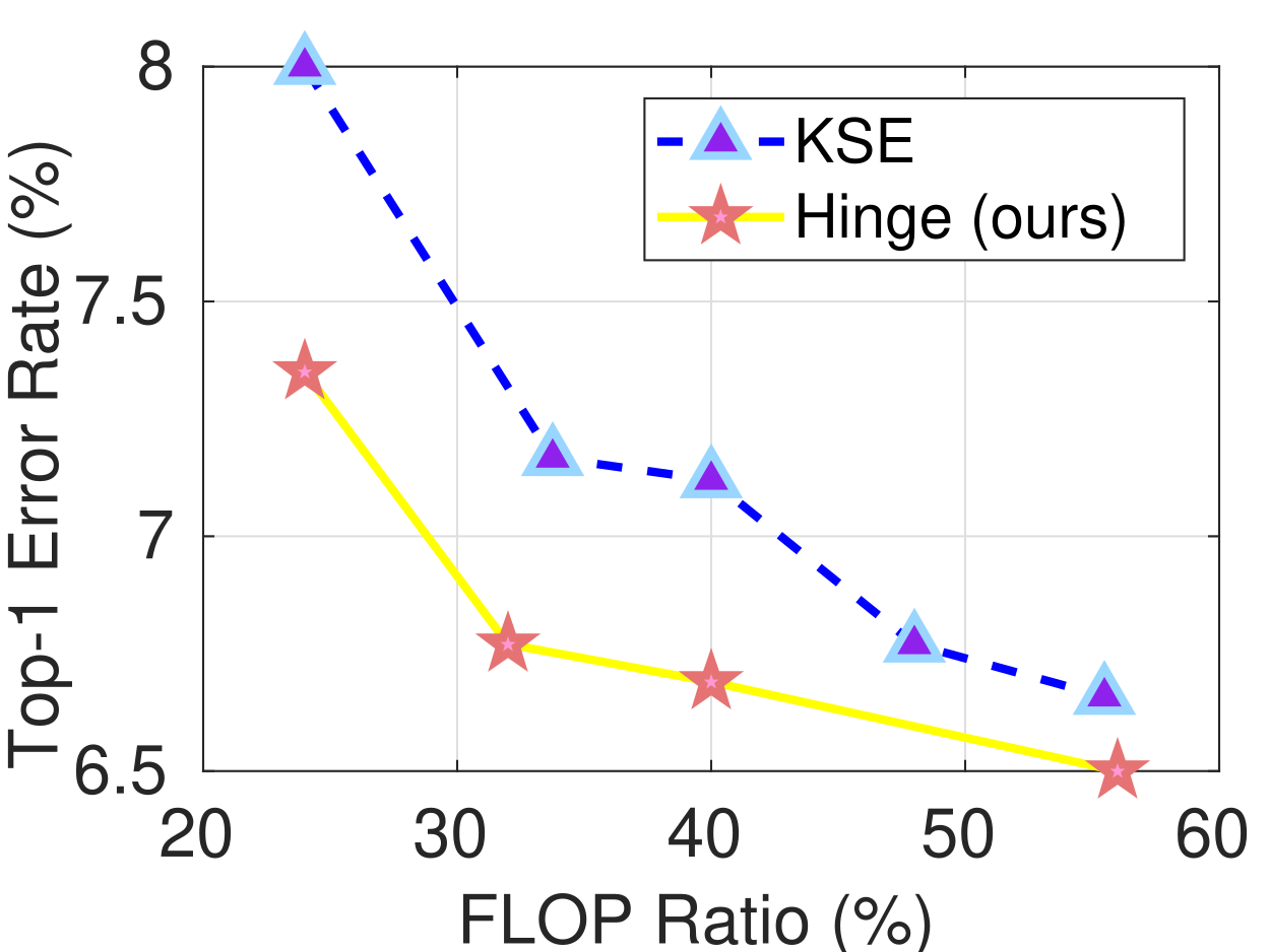
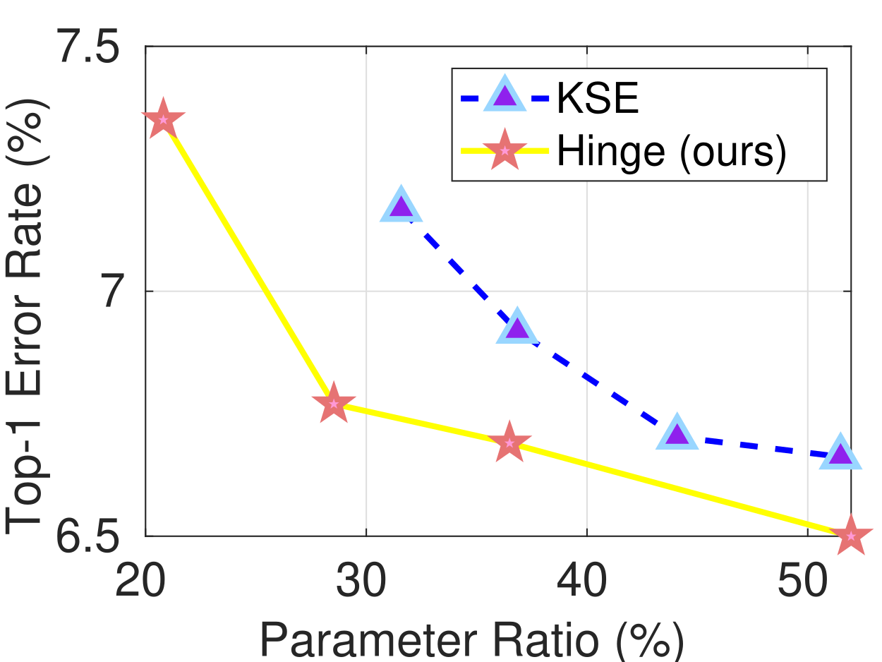
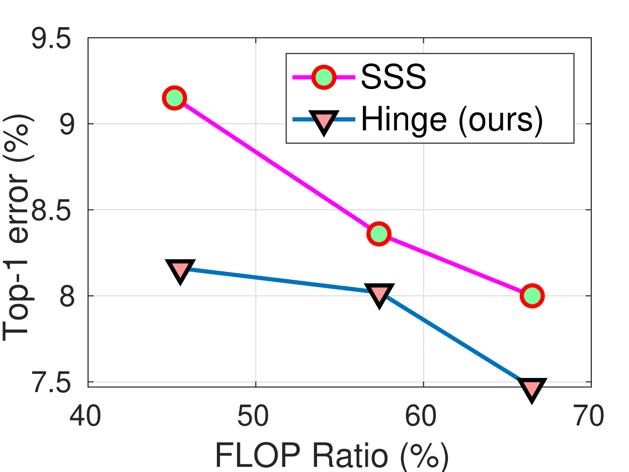
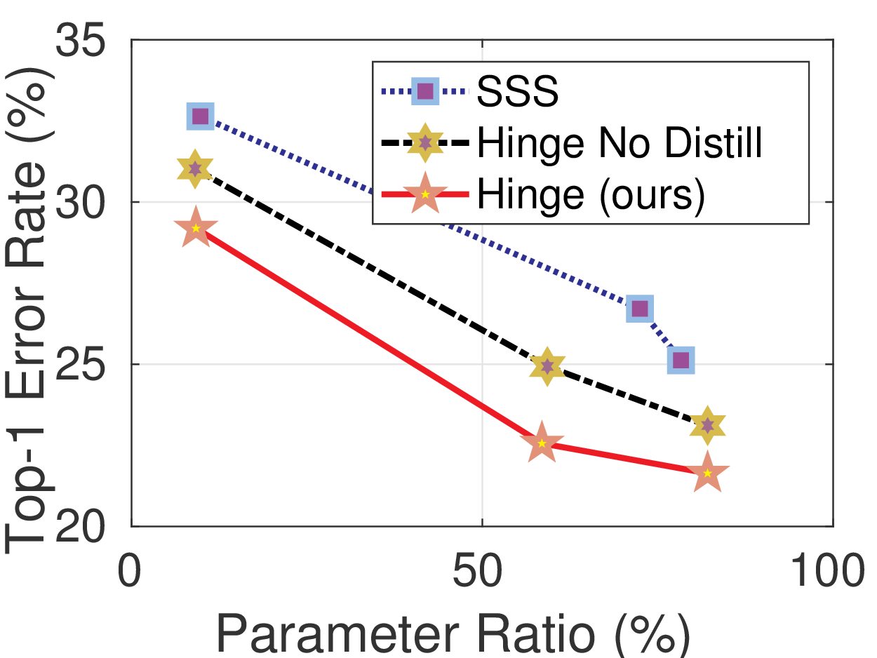
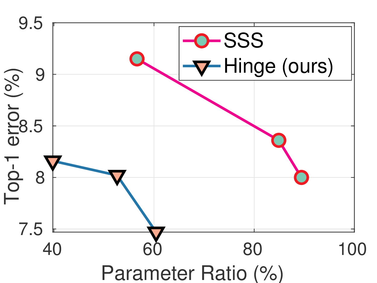
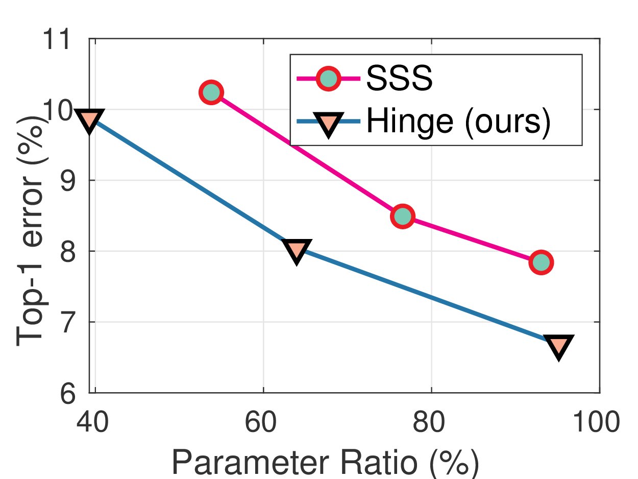
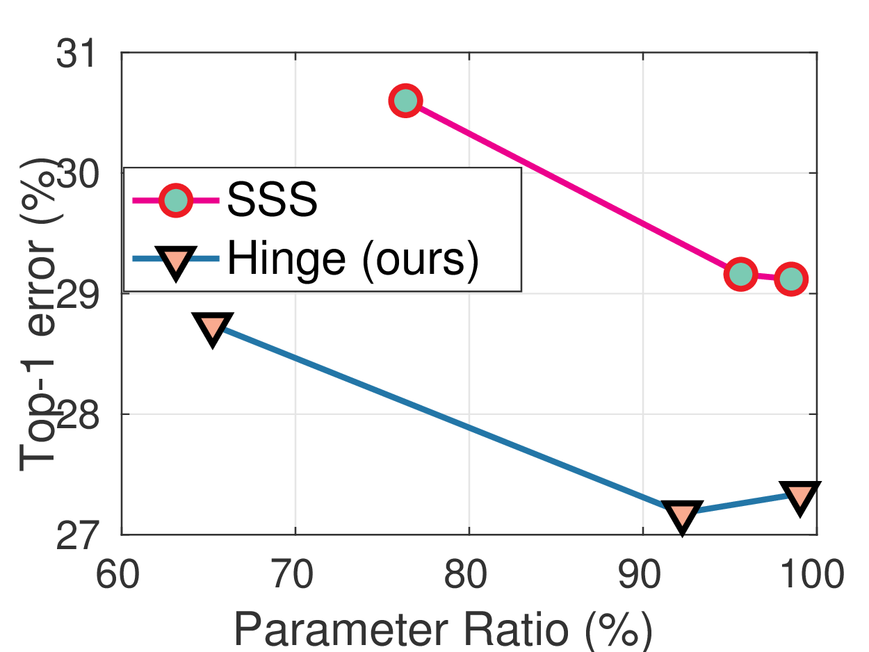
The experimental results on CIFAR10 are shown in Table. 1. The Top-1 error rate, the percentage of the remaining FLOPs and parameters of the compressed models are listed in the table. For ResNet56, two operating points are reported. The operating point of 50% FLOP compression is investigated by a bunch of state-of-the-art compression methods. Our proposed method achieves the best performance under this constraint. At the compression ratio of 24%, our approach is clearly better than KSE [28]. For ResNet and ResNeXt with 20 and 164 layers, our method shoots a lower error rate than SSS. For VGG and DenseNet, the proposed method reduces the Top-1 error rate by 0.41 % and 1.51 % compared with [56]. In Fig. 4, we compare the FLOPs and number of parameters of the compressed model by KSE and the proposed method under different compression ratios. As shown in the figure, our compression method outperforms KSE easily. Fig. 10 and 10 show more comparison between SSS and our methods on CIFAR10. Our method forms a lower bound for SSS.
The ablation study on ResNet56 is shown in Table 3. Different combinations of the hyper parameters and are investigated. There are only slight changes in the results for different combinations. Anyway, when and , our method achieves the lowest error rate. And we use this combination for the other experiments. As for the different regularizers, and regularization are clearly better than and . Due to the simplicity of the solution to the proximal operator of regularization, we use instead of in the other experiments.
5.2 Results on CIFAR100
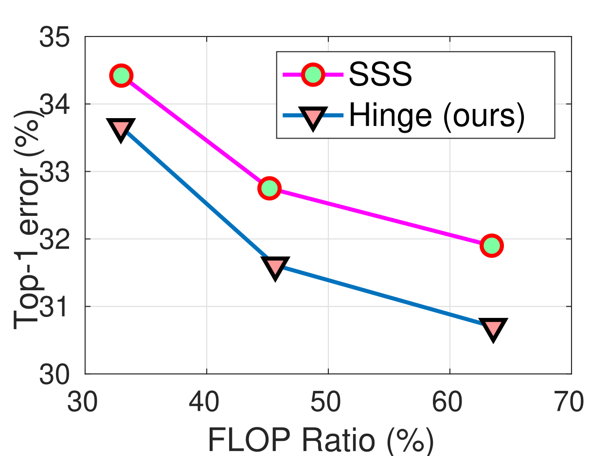
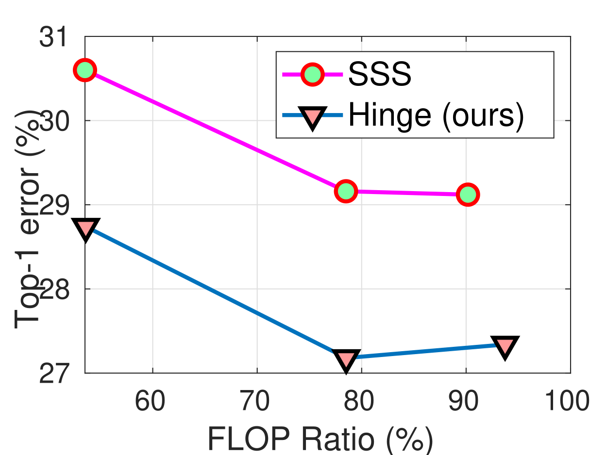
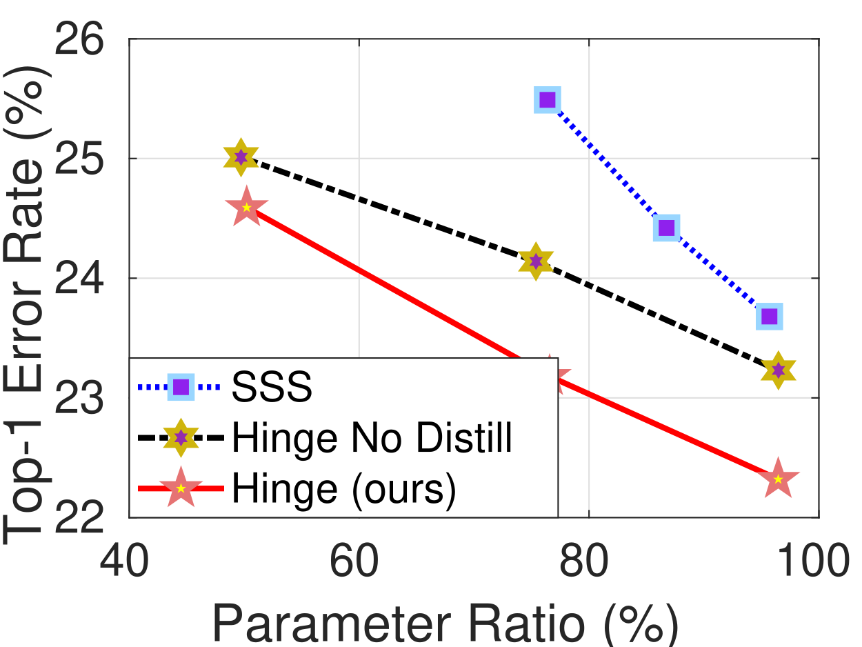
Table 2 shows the compression results on CIFAR100. For the compression of WRN, we analyze the influence of regularization factor annealing during the compression phase. It is clear that with the annealing mechanism, the proposed method achieves much better performance. This is because towards the end of the compression phase, the proximal gradient solver has found quite a good neighbor of the local minimum. In this case, the regularization factor should diminish in order for a better exploration around the local minimum. Compared with the previous group sparsity method CGES [50], our hinge method with the annealing mechanism results in better performance.
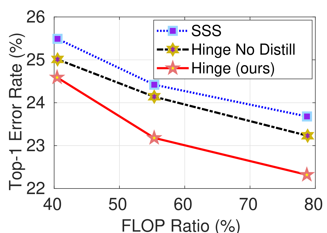
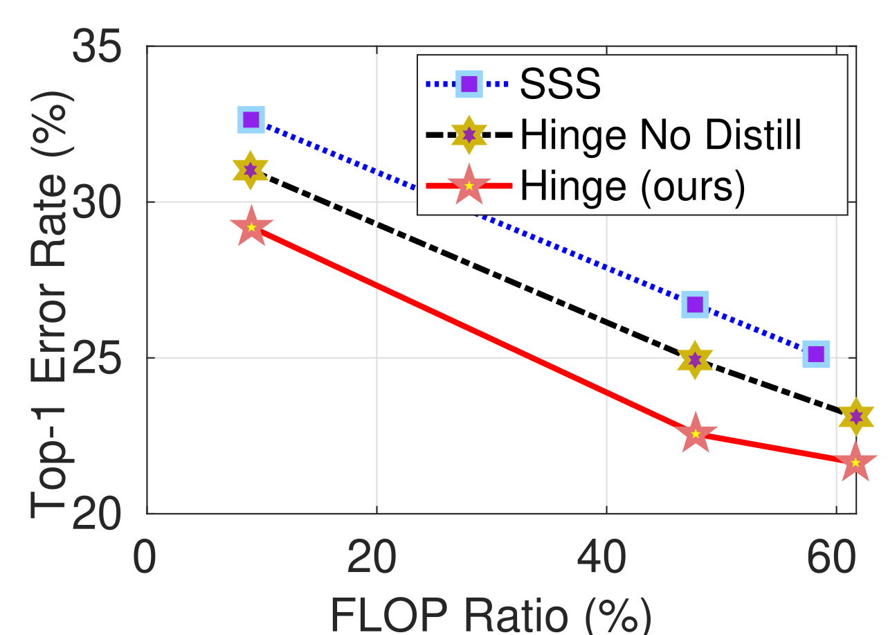
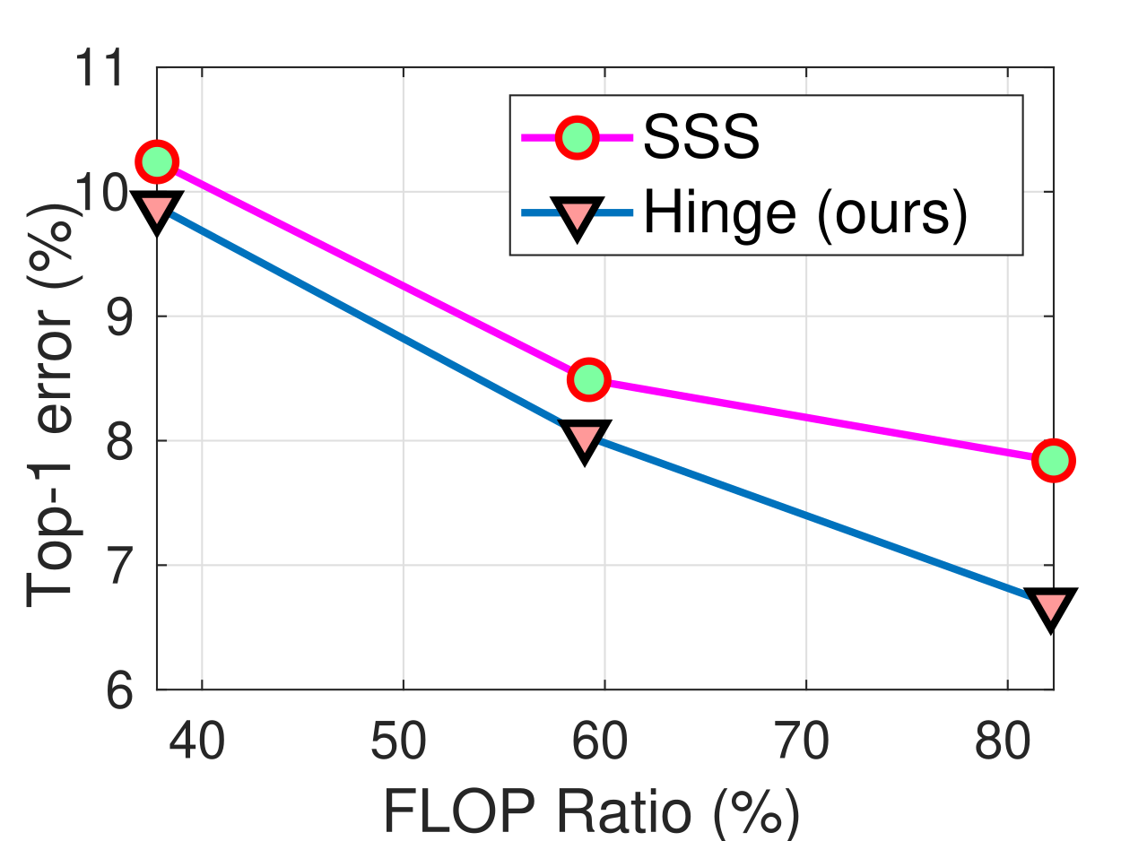
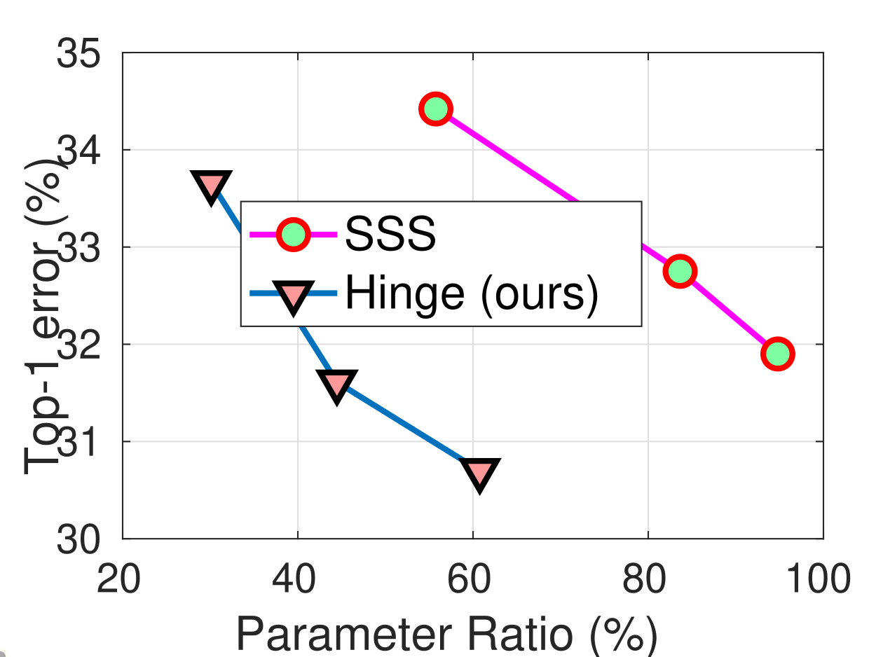
Fig. 5 compares the SSS and our method for the 164-layer networks. Even without the distillation loss, our method is already better than SSS. When the distillation loss is utilized, the proposed method brings the Top-1 error rate to an even lower level. The corresponding results for the 20-layer networks are shown in Fig. 10 and 10, respectively.
| Regularizer | Threshold | Top-1 error (%) | |
|---|---|---|---|
| 0.001 | 0.05 | 6.54 | |
| 0.005 | 0.1 | 6.53 | |
| 0.001 | 0.05 | 6.66 | |
| 0.005 | 0.01 | 6.37 | |
| 0.005 | 0.01 | 6.53 | |
| 0.005 | 0.01 | 6.31 | |
| 0.005 | 0.01 | 6.56 |
| Method | Top-1 Error | FLOPs (%) |
|---|---|---|
| SSS [19] | 25.82 | 68.55 |
| ThinNet-70 [34] | 27.96 | 63.21 |
| NISP [51] | 28.01 | 55.99 |
| Taylor-56% [36] | 25.50 | 55.01 |
| FPGM [15] | 25.17 | 47.50 |
| Hinge (ours) | 25.30 | 46.55 |
| RRBP [58] | 27.00 | 45.45 |
| GAL [30] | 28.20 | 44.98 |
5.3 Results on ImageNet
The comparison results of compressing ResNet50 on the ImageNet2012 dataset is shown in Table 4. Since different methods compare the compressed models under different FLOP compression rates, it is only possible to compare different methods under roughly comparable compression rates. Compared with those methods, our method achieves state-of-the-art trade-off performance between Top-1 error rate and FLOP compression ratio.
6 Conclusion
In this paper, we propose to hinge filter pruning and decomposition via group sparsity. By enforcing group sparsity regularization on the different structured groups, i.e., columns and rows of the sparsity-inducing matrix, the manipulation of the tensor breaks down to filter pruning and decomposition, respectively. The unified formulation enables the devised algorithm to flexibly switch between the two modes of network compression, depending on the specific circumstances in the network. Proximal gradient method with gradient based learning rate adjustment, layer balancing, and regularization factor annealing are used to solve the optimization problem. Distillation loss is used in the finetuning phase. The experimental results validate the proposed method.
Acknowledgments: This work was partly supported by the ETH Zürich Fund (OK), by VSS ASTRA, SBB and Huawei projects, and by Amazon AWS and Nvidia GPU grants.
References
- [1] Jose M Alvarez and Mathieu Salzmann. Learning the number of neurons in deep networks. In Proce. NeurIPS, pages 2270–2278, 2016.
- [2] Jose M Alvarez and Mathieu Salzmann. Compression-aware training of deep networks. In Proc. NeurIPS, pages 856–867, 2017.
- [3] Anubhav Ashok, Nicholas Rhinehart, Fares Beainy, and Kris M Kitani. N2N learning: Network to network compression via policy gradient reinforcement learning. In Proc. ICLR, 2018.
- [4] Amir Beck. First-order methods in optimization, volume 25. SIAM, 2017.
- [5] Stephen Boyd, Neal Parikh, Eric Chu, Borja Peleato, Jonathan Eckstein, et al. Distributed optimization and statistical learning via the alternating direction method of multipliers. Foundations and Trends® in Machine learning, 3(1):1–122, 2011.
- [6] Elliot J Crowley, Gavin Gray, and Amos J Storkey. Moonshine: Distilling with cheap convolutions. In Proc. NeurIPS, pages 2888–2898, 2018.
- [7] Martin Danelljan, Goutam Bhat, Fahad Shahbaz Khan, and Michael Felsberg. ECO: Efficient convolution operators for tracking. In Proc. CVPR, pages 6638–6646, 2017.
- [8] Jia Deng, Wei Dong, Richard Socher, Li-Jia Li, Kai Li, and Li Fei-Fei. ImageNet: A large-scale hierarchical image database. In Proc. CVPR, pages 248–255. IEEE, 2009.
- [9] Emily L Denton, Wojciech Zaremba, Joan Bruna, Yann LeCun, and Rob Fergus. Exploiting linear structure within convolutional networks for efficient evaluation. In Proc. NeurIPS, pages 1269–1277, 2014.
- [10] Shuhang Gu, Qi Xie, Deyu Meng, Wangmeng Zuo, Xiangchu Feng, and Lei Zhang. Weighted nuclear norm minimization and its applications to low level vision. IJCV, 121(2):183–208, 2017.
- [11] Song Han, Huizi Mao, and William J Dally. Deep compression: Compressing deep neural networks with pruning, trained quantization and Huffman coding. In Proc. ICLR, 2015.
- [12] Song Han, Jeff Pool, John Tran, and William Dally. Learning both weights and connections for efficient neural network. In Proc. NeurIPS, pages 1135–1143, 2015.
- [13] Kaiming He, Xiangyu Zhang, Shaoqing Ren, and Jian Sun. Deep residual learning for image recognition. In Proc. CVPR, pages 770–778, 2016.
- [14] Yihui He, Ji Lin, Zhijian Liu, Hanrui Wang, Li-Jia Li, and Song Han. AMC: AutoML for model compression and acceleration on mobile devices. In Proc. ECCV, pages 784–800, 2018.
- [15] Yang He, Ping Liu, Ziwei Wang, Zhilan Hu, and Yi Yang. Filter pruning via geometric median for deep convolutional neural networks acceleration. In Proc. CVPR, pages 4340–4349, 2019.
- [16] Yihui He, Xiangyu Zhang, and Jian Sun. Channel pruning for accelerating very deep neural networks. In Proc. ICCV, pages 1389–1397, 2017.
- [17] Geoffrey Hinton, Oriol Vinyals, and Jeff Dean. Distilling the knowledge in a neural network. arXiv preprint arXiv:1503.02531, 2015.
- [18] Gao Huang, Zhuang Liu, Laurens van der Maaten, and Kilian Q Weinberger. Densely connected convolutional networks. In Proc. CVPR, pages 2261–2269, 2017.
- [19] Zehao Huang and Naiyan Wang. Data-driven sparse structure selection for deep neural networks. In Proc. ECCV, pages 304–320, 2018.
- [20] Max Jaderberg, Andrea Vedaldi, and Andrew Zisserman. Speeding up convolutional neural networks with low rank expansions. In Proc. BMVC, 2014.
- [21] Hyeji Kim, Muhammad Umar Karim Khan, and Chong-Min Kyung. Efficient neural network compression. In Proc. CVPR, June 2019.
- [22] Alex Krizhevsky and Geoffrey Hinton. Learning multiple layers of features from tiny images. Technical report, Citeseer, 2009.
- [23] Alex Krizhevsky, Ilya Sutskever, and Geoffrey E Hinton. Imagenet classification with deep convolutional neural networks. In Proc. NeurIPS, pages 1097–1105, 2012.
- [24] Vadim Lebedev, Yaroslav Ganin, Maksim Rakhuba, Ivan Oseledets, and Victor Lempitsky. Speeding-up convolutional neural networks using fine-tuned CP-decomposition. In Proc. ICLR, 2015.
- [25] Hao Li, Asim Kadav, Igor Durdanovic, Hanan Samet, and Hans Peter Graf. Pruning filters for efficient convnets. In Proc. ICLR, 2017.
- [26] Jiashi Li, Qi Qi, Jingyu Wang, Ce Ge, Yujian Li, Zhangzhang Yue, and Haifeng Sun. OICSR: Out-in-channel sparsity regularization for compact deep neural networks. In Proc. CVPR, pages 7046–7055, 2019.
- [27] Yawei Li, Shuhang Gu, Luc Van Gool, and Radu Timofte. Learning filter basis for convolutional neural network compression. In Proc. ICCV, pages 5623–5632, 2019.
- [28] Yuchao Li, Shaohui Lin, Baochang Zhang, Jianzhuang Liu, David Doermann, Yongjian Wu, Feiyue Huang, and Rongrong Ji. Exploiting kernel sparsity and entropy for interpretable CNN compression. In Proc. CVPR, 2019.
- [29] Yawei Li, Vagia Tsiminaki, Radu Timofte, Marc Pollefeys, and Luc Van Gool. 3D appearance super-resolution with deep learning. In Proc. CVPR, 2019.
- [30] Shaohui Lin, Rongrong Ji, Chenqian Yan, Baochang Zhang, Liujuan Cao, Qixiang Ye, Feiyue Huang, and David Doermann. Towards optimal structured cnn pruning via generative adversarial learning. In Proc. CVPR, pages 2790–2799, 2019.
- [31] Baoyuan Liu, Min Wang, Hassan Foroosh, Marshall Tappen, and Marianna Pensky. Sparse convolutional neural networks. In Proc. CVPR, pages 806–814, 2015.
- [32] Zhuang Liu, Jianguo Li, Zhiqiang Shen, Gao Huang, Shoumeng Yan, and Changshui Zhang. Learning efficient convolutional networks through network slimming. In Proc. ICCV, pages 2736–2744, 2017.
- [33] Jonathan Long, Evan Shelhamer, and Trevor Darrell. Fully convolutional networks for semantic segmentation. In Proc. CVPR, pages 3431–3440, 2015.
- [34] Jian-Hao Luo, Jianxin Wu, and Weiyao Lin. ThiNet: A filter level pruning method for deep neural network compression. In Proc. ICCV, pages 5058–5066, 2017.
- [35] Breton Minnehan and Andreas Savakis. Cascaded projection: End-to-end network compression and acceleration. In Proc. CVPR, June 2019.
- [36] Pavlo Molchanov, Arun Mallya, Stephen Tyree, Iuri Frosio, and Jan Kautz. Importance estimation for neural network pruning. In Proc. CVPR, pages 11264–11272, 2019.
- [37] Markus Nagel, Mart van Baalen, Tijmen Blankevoort, and Max Welling. Data-free quantization through weight equalization and bias correction. In Proc. ICCV, 2019.
- [38] Neal Parikh, Stephen Boyd, et al. Proximal algorithms. Foundations and Trends® in Optimization, 1(3):127–239, 2014.
- [39] Adam Paszke, Sam Gross, Soumith Chintala, Gregory Chanan, Edward Yang, Zachary DeVito, Zeming Lin, Alban Desmaison, Luca Antiga, and Adam Lerer. Automatic differentiation in PyTorch. 2017.
- [40] Joseph Redmon, Santosh Divvala, Ross Girshick, and Ali Farhadi. You only look once: Unified, real-time object detection. In Proc. CVPR, pages 779–788, 2016.
- [41] Karen Simonyan and Andrew Zisserman. Very deep convolutional networks for large-scale image recognition. arXiv preprint arXiv:1409.1556, 2014.
- [42] Sanghyun Son, Seungjun Nah, and Kyoung Mu Lee. Clustering convolutional kernels to compress deep neural networks. In Proc. ECCV, pages 216–232, 2018.
- [43] Amirsina Torfi, Rouzbeh A Shirvani, Sobhan Soleymani, and Naser M Nasrabadi. GASL: Guided attention for sparsity learning in deep neural networks. arXiv preprint arXiv:1901.01939, 2019.
- [44] Frederick Tung and Greg Mori. Similarity-preserving knowledge distillation. In Proc. CVPR, pages 1365–1374, 2019.
- [45] Kuan Wang, Zhijian Liu, Yujun Lin, Ji Lin, and Song Han. HAQ: Hardware-aware automated quantization with mixed precision. In Proc. CVPR, pages 8612–8620, 2019.
- [46] Wei Wen, Chunpeng Wu, Yandan Wang, Yiran Chen, and Hai Li. Learning structured sparsity in deep neural networks. In Proc. NeurIPS, pages 2074–2082, 2016.
- [47] Saining Xie, Ross Girshick, Piotr Dollár, Zhuowen Tu, and Kaiming He. Aggregated residual transformations for deep neural networks. In Proc. CVPR, pages 1492–1500, 2017.
- [48] Zongben Xu, Xiangyu Chang, Fengmin Xu, and Hai Zhang. regularization: A thresholding representation theory and a fast solver. TNNLS, 23(7):1013–1027, 2012.
- [49] Quanming Yao, James T Kwok, and Xiawei Guo. Fast learning with nonconvex L1-2 regularization. arXiv preprint arXiv:1610.09461, 2016.
- [50] Jaehong Yoon and Sung Ju Hwang. Combined group and exclusive sparsity for deep neural networks. In Proc. ICML, pages 3958–3966. JMLR. org, 2017.
- [51] Ruichi Yu, Ang Li, Chun-Fu Chen, Jui-Hsin Lai, Vlad I Morariu, Xintong Han, Mingfei Gao, Ching-Yung Lin, and Larry S Davis. NISP: Pruning networks using neuron importance score propagation. In Proc. CVPR, pages 9194–9203, 2018.
- [52] Sergey Zagoruyko and Nikos Komodakis. Wide residual networks. 2016.
- [53] Dejiao Zhang, Haozhu Wang, Mario Figueiredo, and Laura Balzano. Learning to share: Simultaneous parameter tying and sparsification in deep learning. In Proc. ICLR, 2018.
- [54] Kai Zhang, Wangmeng Zuo, Yunjin Chen, Deyu Meng, and Lei Zhang. Beyond a gaussian denoiser: residual learning of deep CNN for image denoising. IEEE TIP, 26(7):3142–3155, 2017.
- [55] Xiangyu Zhang, Jianhua Zou, Kaiming He, and Jian Sun. Accelerating very deep convolutional networks for classification and detection. IEEE TPAMI, 38(10):1943–1955, 2015.
- [56] Chenglong Zhao, Bingbing Ni, Jian Zhang, Qiwei Zhao, Wenjun Zhang, and Qi Tian. Variational convolutional neural network pruning. In Proc. CVPR, pages 2780–2789, 2019.
- [57] Hao Zhou, Jose M Alvarez, and Fatih Porikli. Less is more: Towards compact cnns. In Proc. ECCV, pages 662–677. Springer, 2016.
- [58] Yuefu Zhou, Ya Zhang, Yanfeng Wang, and Qi Tian. Accelerate cnn via recursive bayesian pruning. In Proc. CVPR, pages 3306–3315, 2019.
Supplementary Material for “Group Sparsity: The Hinge Between Filter Pruning and Decomposition for Network Compression”
Appendix A Closed-form Solutions to the Proximal Operators
The proximal operator of a given function is defined by
| (10) |
This operator has closed-form solution when the function has the form of , , , and regularization. For , the solution is the soft-thresholding function and for it is the so-called half-thresholding function. The soft-thresholding function is defined as
| (11) |
where is the sign function and calculates the maximum of the argument and 0. The hard-thresholding function is given by
| (12) |
where .
The group sparsity regularizer is defined as
| (13) |
where is the function of the group norms and has the form of norm here. The proximal operator of the sparsity-inducing matrix defined in the main paper is
| (14) |
where the function replaces in Eqn. 10. The closed-form solution of the proximal operator in Eqn. 14 can be derived from the solutions to Eqn. 10 according to the following theorem [4].
Theorem 1
Let be a function given by , where is a proper closed and convex function satisfying . Then,
| (15) |
Thus, with a little bit variable substitution, when is regularizer, the solution to Eqn. 14 is given by
| (16) |
where is the -th element in the -th group of the sparsity-inducing matrix , and for the sake of simplicity, the subscript t+Δ is omitted.
When the function has the form of , , and , it is non-convex. However, we still use the variable substitution in Theorem 15 experimentally and the corresponding results in the main paper are also very competitive. For regularizer, the solution is given by
| (17) |
where . Similarly, the solution to the regularizer is given by
| (18) |
where , , , and . When the regularizer is regularizer, then the solution is given by
| (19) |
where . Note that the case where all of the group norms equal 0 is not considered [49] because it never happens during the optimization of our algorithm. The solutions are summarized in Table 5.
| Regularizer | Solution |
|---|---|
| , , , |
| Regularizer | ||||
|---|---|---|---|---|
| Regularization factor |
Appendix B Hyper Parameters for Different Regularizers
The regularization factors for different regularizers are listed in Table 6. For CIFAR10 and CIFAR100 datasets, the learning rate of the sparsity-inducing matrix during compression optimization is set to 0.1. The ratio between the learning rate of and is set to 0.01. That is, the learning rate of during compression optimization is 0.001. For ImageNet, both and during optimization are set to 0.001.
Appendix C More Parameter Comparison
In Fig. 9 and Fig. 10, more parameter comparison results are shown. The figures report several operating points of the proposed method and SSS [19]. The proposed method forms a lower error bound for SSS. In Fig. 9, our Hinge method without distillation loss is already better than SSS. And with the distillation loss, the proposed method shoots even lower Top-1 error rate.
Appendix D Layer-wise Compression Ratio
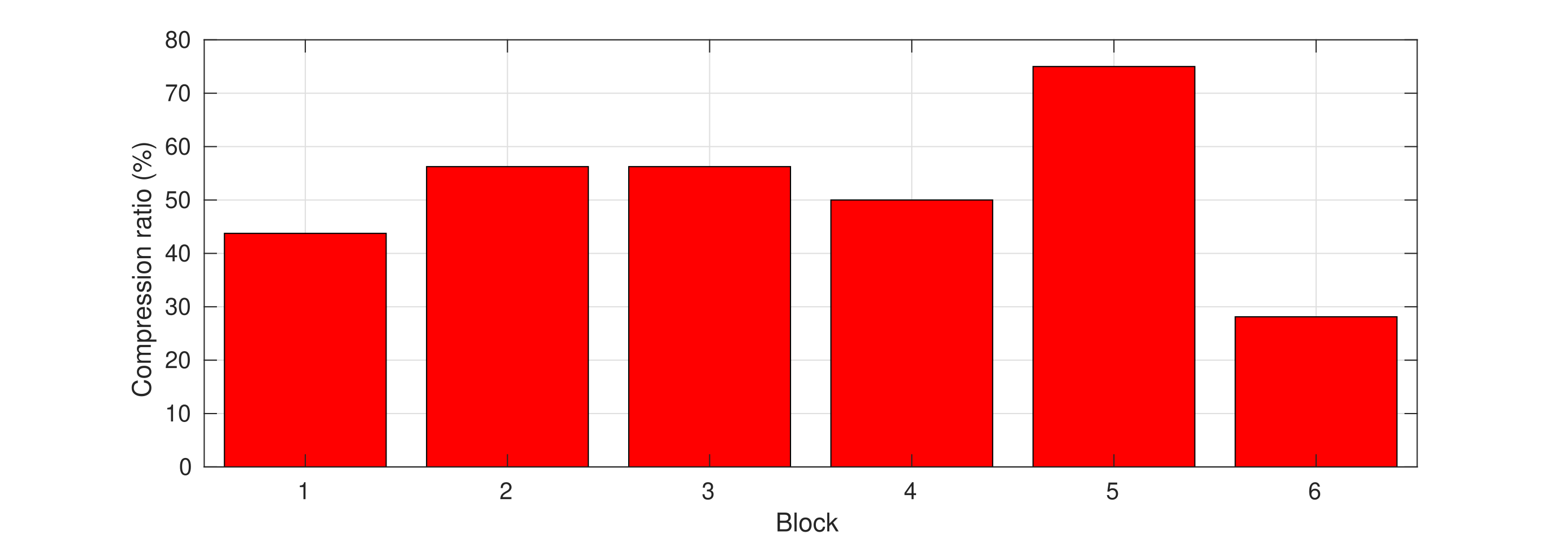
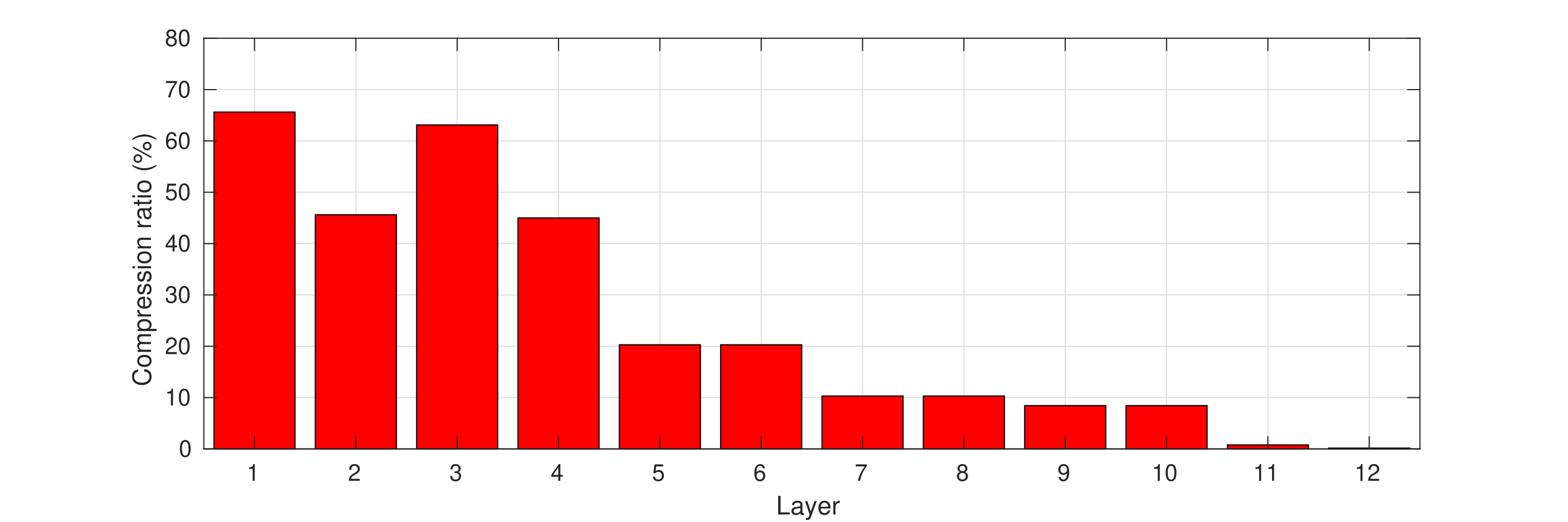
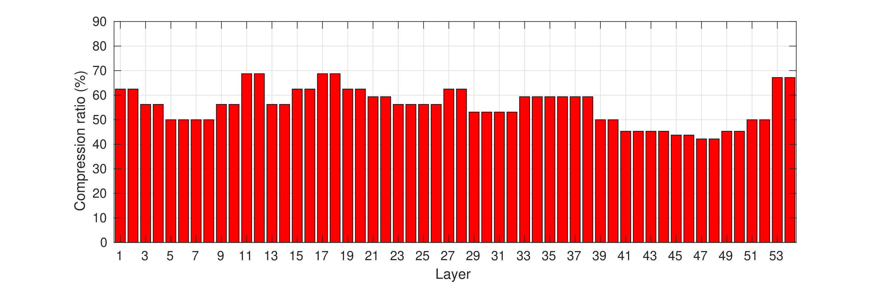
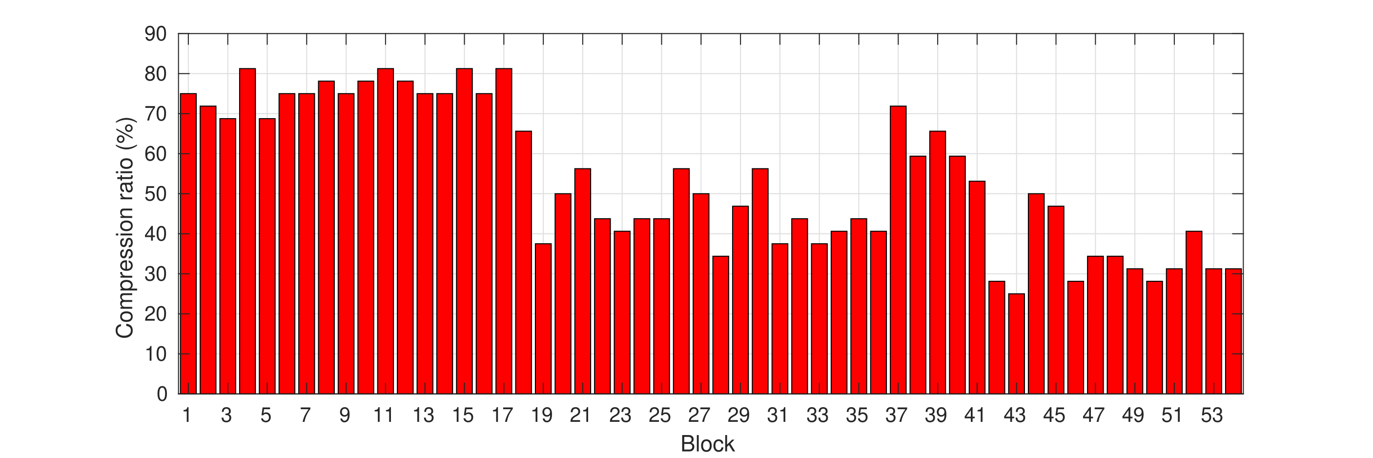
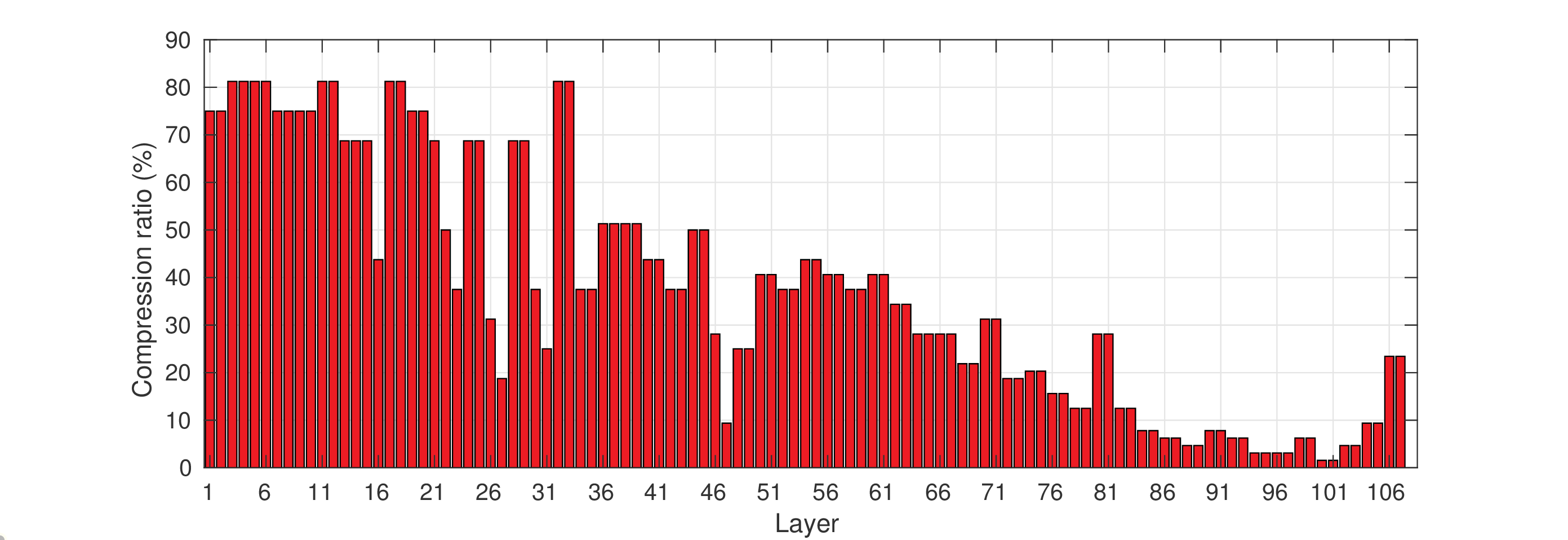
The layer-wise or block-wise compression ratio of the model compressed by the proposed method is shown in Fig. 7 and Fig. 8, respectively. For ResNeXt [47], the aim is to compress the convolution in the residual block and the two convolutions are used as the sparsity-inducing matrices. Thus, the block-wise compression ratio is reported. For ResNet [13] and WRN [52], there are two convolutions in each residual block. Each of the two convolutions is compressed by introducing a sparsity-inducing matrix. Thus, the layer-wise compression ratio is reported. As shown in the Fig. 7, Fig. 8 and Fig. 8, for WRN, ResNeXt164, and ResNet164, our approach tends to compress the shallow layers more compared with the deep layers. This is consistent with former research [16]. As for ResNet56 in Fig 7, the proposed method results in a sawtooth architecture. That is, for the convolutions with the same feature dimension (i.e. Layer 1 to Layer 18, Layer 19 to Layer 36, and Layer 37 to Layer54), the middle layers generally have a severer degree of compression.