Formal Synthesis of Lyapunov Neural Networks

Abstract

We propose an automatic and formally sound method for synthesising Lyapunov functions for the asymptotic stability of autonomous non-linear systems. Traditional methods are either analytical and require manual effort or are numerical but lack of formal soundness. Symbolic computational methods for Lyapunov functions, which are in between, give formal guarantees but are typically semi-automatic because they rely on the user to provide appropriate function templates. We propose a method that finds Lyapunov functions fully automatically—using machine learning—while also providing formal guarantees—using satisfiability modulo theories (SMT). We employ a counterexample-guided approach where a numerical learner and a symbolic verifier interact to construct provably correct Lyapunov neural networks (LNNs). The learner trains a neural network that satisfies the Lyapunov criteria for asymptotic stability over a samples set; the verifier proves via SMT solving that the criteria are satisfied over the whole domain or augments the samples set with counterexamples. Our method supports neural networks with polynomial activation functions and multiple depth and width, which display wide learning capabilities. We demonstrate our method over several non-trivial benchmarks and compare it favourably against a numerical optimisation-based approach, a symbolic template-based approach, and a cognate LNN-based approach. Our method synthesises Lyapunov functions faster and over wider spatial domains than the alternatives, yet providing stronger or equal guarantees.

I Introduction

Stability analysis determines whether a dynamical system never escapes a domain of interest around an equilibrium point and, possibly, converges asymptotically towards the point. Stability properties constitute a primary objective for control engineering, yet designing controllers for systems that are highly complex is error prone. Automatic stability analysis computes certificates of stability whose aim is providing correctness guarantees to the traditional workflow. We address the stability analysis of systems with given controllers or, more generally, autonomous systems described by non-linear ordinary differential equations (ODEs). In particular, we present a novel method for the automated and formal synthesis of Lyapunov functions.

Lyapunov functions are formal certificates for the asymptotic stability of ODEs. We consider autonomous $n$-dimensional systems of non-linear ODEs

$$\dot{x}=f(x),\quad x\in\mathbb{R}^{n},$$ (1)

having an equilibrium point at $x_{e}$ and a domain of interest $\mathcal{D}\subseteq\mathbb{R}^{n}$ containing $x_{e}$. A Lyapunov function is a real-valued function $V:\mathbb{R}^{n}\to\mathbb{R}$ such that $V(x_{e})=0$ and, for all states $x\in\mathcal{D}$ other than $x_{e}$, it satisfies the two conditions

$$\dot{V}(x)=\nabla V(x)\cdot f(x)<0, V(x)>0.$$ (2)

A Lyapunov function maps system states $x$ into energy-like values that, by the first condition, decrease over time along the model’s trajectories and, by the second condition, are bounded from below. If one such function exists, then the system is asymptotically stable within $\mathcal{D}$.

Finding a Lyapunov function is in general a hard problem and has been the objective of numerous studies. In standard literature Lyapunov functions are constructed via analytical methods, which are mathematically sound but require substantial expertise and manual effort. Algorithmically, for linear ODEs it is sufficient to use quadratic programming, as Lyapunov functions are necessarily quadratic polynomials. However, for non-linear ODEs no general method to automatically construct Lyapunov functions exists [6].

Numerical methods for non-linear autonomous systems include techniques that reduce the problem to solving a partial differential equations (PDEs), partition and linearise the vector field $f$ and then reformulate the problem as a linear program (LP), or restrict $V$ to be a sum-of-squares (SOS) function and relax the synthesis problem into a linear matrix inequalities (LMI) program [13]. Despite their analytical exactness, PDE-based methods rely on numerical integrators which are bound to machine precision, LP-based methods linearise $f$ with finite accuracy, and LMI-based methods employ numerical convex optimisation—unfortunately, all these methods are numerically unsound. Conversely, we deal with constructing a Lyapunov function as a problem of formal synthesis, which is not only automatic, but also formally sound.

Formal methods for the synthesis of Lyapunov functions guarantee the formal correctness of their result using satisfiability modulo theories (SMT) or a computer algebra system (CAS). Typically, formal methods assume $V$ to be given in some parameterised form, i.e., a template (a.k.a. sketch), and either relax the entire problem into a computationally tractable abstraction or incrementally construct and check candidates in a counterexample-guided inductive synthesis (CEGIS) fashion [24]. Relaxation-based methods typically assume polynomial templates and reformulate the problem as a semi-algebraic one [23, 22] or as a linear program [16, 19, 20] and solve them using a CAS or SMT; notably, Darboux-based semi-algebraic methods can also relax problems with transcendental functions [7]. Alternatively, incremental methods construct, from polynomial templates, candidates for $V$ using linear relaxations [17], genetic algorithms [25], fitting simulations or, more directly, spatial samples [9, 3]; then, they verify the candidates using a CAS or SMT and, whenever necessary, refine the search space by learning from generated counterexamples. Notably, all methods rely on the user to provide a good template expression. We overcome the limit of manually selecting a template using, instead of fixed expressions, generic templates based on neural networks.

Neural networks are widely used in a variety of applications, such as in image classification and in natural language processing. Neural networks are powerful regressors and thus lend themselves to the approximation of Lyapunov functions [10, 15]. The construction of Lyapunov neural networks (LNNs) has been previously studied by approaches based on simulations and numerical optimisation, all of which are formally unsound [21, 14, 12, 18, 11].

We introduce a method that exploits efficient machine learning algorithms, while guaranteeing formal soundness. We follow a CEGIS procedure, where first a numerical learner trains an LNN candidate to satisfy the Lyapunov conditions (Eq. (2)) over a samples set and then a formal verifier confirms or falsifies whether the conditions are satisfied over the whole dense domain. If the verifier falsifies the candidate, one or more counterexamples are added to the samples set and the network is retrained. The procedure repeats in a loop until the verifier confirms the LNN. Our learner trains neural networks with multiple layers and polynomial activations functions of any degree; on the technical side, learning enjoys better performance when the last layer has quadratic activation. Our verifier guarantees the formal correctness of the results using a sound decision procedure for SMT over theories for polynomial constraints [5, 8]. Besides, the previous CEGIS methods for LNNs provide weaker guarantees, namely Lagrange (practical) stability, which excludes a neighbourhood around the equilibrium $x_{e}$ [4]—conversely, our novel method guarantees full asymptotic stability at $x_{e}$.

We have built a prototype software and compared our method against a numerical LMI-based method (SOSTOOLS) [13], a formal template-based CEGIS method [3], and the cognate CEGIS approach for LNNs [4]. We have evaluated their performance over four systems of polynomial ODEs that are challenging as do not admit polynomial Lyapunov functions over the entire $\mathbb{R}^{n}$. We have thus measured the widest domain for which each of the methods succeeded to find a Lyapunov function. Our method has attained comparable or wider domains than the other approaches, in shorter or comparable time. Notably, our method gives the strongest guarantees within the alternatives (asymptotic stability) and does not rely on user hints.

Altogether, we present a synthesis method for LNNs that (i) accounts for the asymptotic stability of systems of non-linear ODEs, (ii) is sound and automatic, and (iii) is faster and covers wider domains than other state-of-the-art tools.

II Counterexample-guided Inductive Synthesis of Lyapunov Neural Networks

Figure 1: A feed-forward neural network with one hidden layer.

We introduce a CEGIS procedure for the construction of Lyapunov functions in the form of feed-forward neural networks. We consider a network with a number $n$ of input neurons that corresponds with the dimension of the dynamical system, followed by $k$ hidden layers with respectively $h_{1},\dots,h_{k}$ neurons, and finally followed by one output neuron. Nodes of adjacent layers are fully interconnected: a matrix $W_{1}\in\mathbb{R}^{h_{1}\times n}$ encompasses the weights from input to first hidden layer, a matrix $W_{i}\in\mathbb{R}^{h_{i}\times h_{i-1}}$ the weights from any other $(i-1)$-th to $i$-th hidden layer, and a matrix $W_{k+1}\in\mathbb{R}^{1\times h_{k}}$ the weights from $k$-th layer to the last neuron. Neurons have no additive bias. Every $i$-th hidden layer comes with a non-linear activation function $\sigma_{i}\colon\mathbb{R}\to\mathbb{R}$ and the output neuron is activation free. The valuation of output and hidden layers are given by

$$z_{k+1}=W_{k+1}z_{k}, z_{i}=\sigma_{i}(W_{i}z_{i-1}), i=1,\dots,k,$$ (3)

where each $\sigma_{i}$ is applied element-wise to its $h_{i}$-dimensional argument and $z_{0}$ is the input layer. Upon assigning the argument $x\in\mathbb{R}^{n}$ to the input layer, the neural network evaluates Eq. (3) layer by layer, resulting in the function

$$V(x)=z_{k+1}, z_{0}=x.$$ (4)

Figure 1 depicts a neural network of this kind with $k=1$, $n=h_{1}=2$, and the weights $w_{1},\dots,w_{6}$. Unlike the standard definition, we assume here to have no additive bias and require $\sigma_{i}(0)=0$ for $i=1,\dots,k$, which results in the condition $V(0)=0$.

Figure 2: CEGIS architecture for the synthesis of LNNs.

Our procedure takes as input an $n$-dimensional vector field $f\colon\mathbb{R}^{n}\to\mathbb{R}^{n}$ with equilibrium point (w.l.o.g.) $x_{e}=0$, a domain $\mathcal{D}\subseteq\mathbb{R}^{n}$, and the desired depth $k$ and width $h_{1},\dots,h_{k}$ for the hidden layers of the network. Upon termination, the procedure returns a neural network $V\colon\mathbb{R}^{n}\to\mathbb{R}$ that satisfies the Lyapunov conditions in Eq. (2), which is an LNN for the asymptotic stability of $f$ within region $\mathcal{D}$.

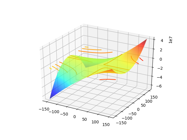
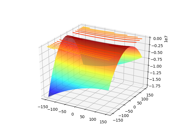
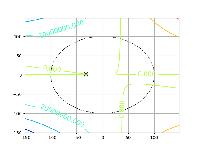
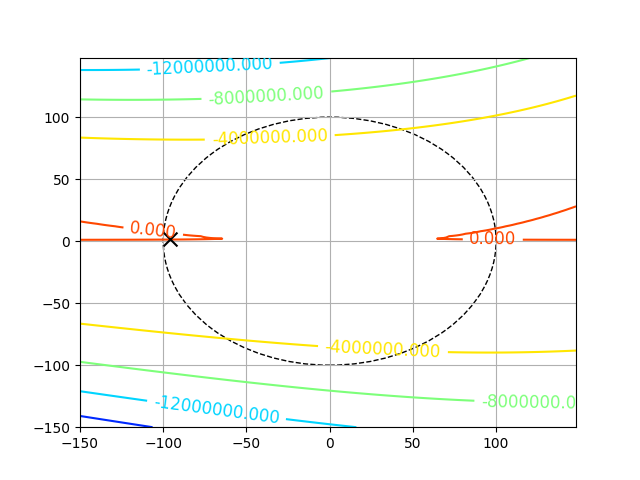
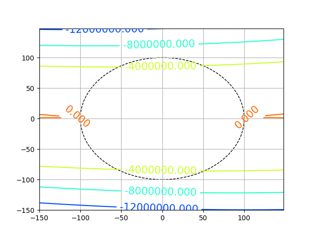
Initial guess.	After the first counterexample.	After the second counterexample.
(a)	(b)	(c)

Figure 3: The evolution of $\dot{V}(x,y)$ with the corresponding level sets through three CEGIS iterations for certifying the asymptotic stability of the system in Eq. 5 within a circle of radius $\gamma=100$, using the neural network in Fig. 1. The synthesis loop finds two counterexamples, shown as crosses, and succeeds after three iterations.

Figure 2 outlines the architecture which consists of a learner and a formal verifier interacting in a CEGIS loop. The learner trains a candidate neural network $V$ to satisfy the conditions in Eq. (2) over a discrete set of samples $S\subset\mathcal{D}$, which is initialised randomly. The outcome from the learner satisfies $V(0)=0$, $\dot{V}(s)<0$, and $V(s)>0$ over all samples $s\in S$, but not necessarily over the entire dense domain $\mathcal{D}$. Thus the formal verifier checks whether the resulting $V$ violates the same conditions within the whole $\mathcal{D}$ and, if so, produces a set of samples $C\subset\mathcal{D}$ containing one or more counterexamples $c$ that violate either $\dot{V}(c)<0$ or $V(c)>0$. We add $C$ to the samples set $S$, hence forcing the learner to newly produce a different candidate function, which will later be passed again to the verifier. The loop repeats indefinitely, until the verifier proves that no counterexamples exist: this outcome proves that $V$ is an LNN over the entire $\mathcal{D}$. We cannot however guarantee termination of this procedure in general, rather we are interested in its performance in practice.

Example

We demonstrate the workflow of our procedure with the planar dynamical system described by

$$\left\{\begin{array}[]{l}\dot{x}=-x+xy\\ \dot{y}=-y.\end{array}\right.$$ (5)

The system is asymptotically stable at the origin [2]. We aim at proving its stability within the circle of radius 100 centred at the origin, that is $\mathcal{D}=\{x\colon||x||_{2}\leq\gamma\}$ for $\gamma=100$. First, we select the neural network in Fig. 1, for which $k=1$ and $h_{k}=2$, and use the quadratic activation function $\sigma_{1}(x)=x^{2}$. Second, we also impose $w_{5}=w_{6}=1$, which makes the training of $V$ faster (see Sec. III). Finally, our CEGIS procedure trains a provably correct LNN after three learner/verifier iterations; Figure 3 shows the evolution of $\dot{V}$ after each iteration. At the beginning, the procedure samples a set $S$ of random points from $\mathcal{D}$ and then invokes the learner. The learner keeps the samples in state space fixed, while it searches over the parameter space $w_{1},\dots,w_{4}$ using numerical gradient descent. In particular, it computes a network candidate that satisfies the Lyapunov conditions for all random initial points: the result is shown in Fig. 3a. Next, the verifier fixes the current instance of parameters $w_{1},\dots,w_{4}$ as constants, and the SMT solver accepts a first-order logic formula whose variables are the state-space points $x\in\mathcal{D}$ that violate the Lyapunov conditions. The solution returned by the SMT solver is the counterexample $c$ that is depicted in Fig. 3a as a cross, for which $\dot{V}(c)\geq 0$. At the second iteration, the counterexample is added to $S$ and the network retrained over the extended batch, obtaining the $\dot{V}$ of Fig. 3b. Now the network satisfies the conditions over all initial samples plus the newly added point, yet it violates it over a different counterexample, which is depicted in Fig. 3b. The verifier identifies this counterexample and adds it to $S$. At the third and last iteration, the learner retrains the neural network, which yields Fig. 3c. The verifier re-checks it, but this time it fails at producing any counterexamples, thus proving their absence. Consequently, the neural network satisfies the Lyapunov conditions over the entire continuous domain $\mathcal{D}$, and the CEGIS loop terminates successfully. $\square$

The formal synthesis of LNNs consists of finding an instance of weights for which the neural network satisfies the Lyapunov conditions of Eq. (2). Our CEGIS loop tackles this general problem by solving two separate problems interactively: the first is learning and the second is verifying. We capitalise on the power of neural networks for learning from data (see Sec. III), and on the power of SMT solving for verifying or for producing counterexamples accordingly (see Sec. IV).

III Training of Lyapunov Neural Networks

The first active CEGIS component is the learner, which uses gradient descent to train LNN candidates. The learner instantiates a candidate using the hyper-parameters $k$ and $h_{1},\dots,h_{k}$ (depth and width of the network), trains it over the discrete set of samples $S$, and refines its training whenever the verifier adds counterexamples.

The training procedure performs the minimisation of a loss function that depends on $V$ and $\dot{V}$, both evaluated on the data points in $S$. The Lyapunov requirements split the sample set $S$ into two partitions $S^{-}$ and $S^{+}$, such that all points $s\in S^{-}$ satisfy both conditions $\dot{V}(s)<0$ and $V(s)>0$, whereas all data points $s\in S^{+}$ violate either of them. The loss function should penalise all data points in the $S^{+}$partition, while rewarding the $S^{-}$ partition. To this end, we employ the Leaky ReLU function, which is defined as

$$LR(p,a)=\begin{cases}p&\text{if }p\geq 0\\ ap&\text{otherwise,}\end{cases}$$ (6)

where $a$ is a (small) positive constant and $p$ is the variable of interest. We thus minimise the sum of LR over the values $p_{1}=\dot{V}(s)$ and $p_{2}=-V(s)$, as in (7). Additionally, to enhance the numerical stability of the training, we apply a small offset $\varepsilon$ to $p_{1}$ and $p_{2}$, therefore rewarding data points $s$ where $\dot{V}(s)\leq-\varepsilon$ and $V(s)\geq\varepsilon$, and penalising them otherwise. Altogether, our loss function is

$$\mathcal{L}(s)=\underbrace{LR(\dot{V}(s)+\varepsilon,a)}_{\mathcal{L}_{1}}+\underbrace{LR(-{V}(s)+\varepsilon,a)}_{\mathcal{L}_{2}}$$ (7)

where $\mathcal{L}_{1}$ accounts for training $\dot{V}(x)<0$, $\mathcal{L}_{2}$ accounts for training $V(x)>0$, and where $a$ and $\varepsilon$ are hyper-parameters defined above. In contrast to a standard ReLU formulation, a Leaky ReLU rewards $S^{-}$ by $a$, which induces training below zero, improves learning, and yields a numerically robust LNN candidate.

We evaluate the expression of $\dot{V}(x)=\nabla V(x)\cdot f(x)$ directly from the matrices $W_{i}$, thus avoiding a symbolic differentiation of $V(x)$. Let us recall the value of the $i$-th layer, $z_{i}=\sigma_{i}(W_{i}z_{i-1})$, so that $z_{0}=x$, whereas the output layer is activation free, hence $z_{k+1}=W_{k+1}z_{k}$. To compute the gradient of $V(x)$ over $x$ we use the chain rule

$$\nabla V(x)=\frac{\partial V}{\partial x}=\prod_{i=1}^{k+1}\frac{\partial z_{i}}{\partial z_{i-1}}.$$ (8)

After a few algebraic steps, the factors result in

$$\frac{\partial z_{i}}{\partial z_{i-1}}=\frac{\partial\sigma_{i}(W_{i}z_{i-1})}{\partial z_{i-1}}=\text{diag}[\sigma_{i}^{\prime}(W_{i}z_{i-1})]\cdot W_{i},$$ (9)

for $i=1,\dots,k$, whereas for the last layer $\partial z_{k+1}/\partial z_{k}=W_{k+1}$; $\sigma_{i}^{\prime}$ is the full derivative of function $\sigma_{i}$ and $\text{diag}[v]$ represents a diagonal matrix whose entries are the elements of vector $v$. Finally, the gradient results in

$$\nabla V(x)=W_{k+1}\cdot\prod_{i=1}^{k}\text{diag}[\sigma^{\prime}_{i}(W_{i}z_{i-1})]\cdot W_{i}.$$ (10)

We compute the values of $z_{i}$ recursively from $z_{0}=x$ using Eq. (3). For every point $s$ in ${S}$, we thus evaluate $\nabla V(s)$ using simple matrix-vector operations, and, along with the value of $f(s)$, finally obtain $\dot{V}(s)=\nabla V(s)\cdot f(s)$.

Training benefits from candidate networks that satisfy or likely satisfy one of the Lyapunov conditions $\dot{V}(x)<0$ or $V(x)>0$ a priori. An example are neural networks for which the last hidden layer has quadratic activation and positive output, i.e., $\sigma_{k}(x)=x^{2}$ and $W_{k+1}>0$. For a generic selection of weights, these networks are likely to satisfy $V(s)>0$ over the samples $s\in S$. As a result, the component $\mathcal{L}_{2}$ becomes negligible with respect to $\mathcal{L}_{1}$ during most of the training. Imposing these simple conditions to the network improves the overall training performance considerably.

	2	5	10	50	100	200	[5, 2]	[5, 5]	[10, 5]	[50, 10]	[100, 50]
$10$	0.06	0.14	0.23	1.63	1.87	11.41	0.56	1.62	2.28	3.68	9.74
$20$	0.14	0.67	0.21	2.99	11.85	63.03	8.86	1.34	5.64	14.32	59.28
$50$	0.11	2.27	1.96	7.02	21.65	110.25	121.30	21.78	3.26	82.44	158.09
$100$	3.68	1.90	3.03	11.46	51.63	119.40	oot	oot	222.12	oot	oot
$200$	48.17	23.10	53.17	30.89	165.99	301.71	oot	oot	oot	oot	oot
$500$	oot	70.65	72.09	12.01	33.91	371.65	oot	oot	oot	oot	oot

TABLE I: Performance results in terms of computational time [sec] varying the number of hidden neurons $h$ and the radius $\gamma$ of the domain $\mathcal{D}$. The fastest outcomes for one- and two hidden-layer LNN are highlighted; oot indicates timeout.

IV Verification of LNNs using SMT solving

Satisfiability modulo theories (SMT) comprises diverse methods for deciding the satisfiability of first-order logic formulae. SMT solvers combine combinatorial and symbolic algorithms which, unlike common numerical solvers and optimisers, provide formal guarantees about their results that are equivalent to those of analytical proofs. We employ SMT solving for deciding whether a neural network is a Lyapunov function, or for finding counterexamples otherwise, which is the core of our verifier architecture.

Deciding whether a neural network $V$ is a Lyapunov function for a system with equilibrium (w.l.o.g.) $x_{e}=0$ and within the domain $\mathcal{D}$ amounts to deciding the formula

$$\forall x\colon(x\in\mathcal{D}\land x\neq 0)\Rightarrow(\dot{V}(x)<0\land V(x)>0).$$ (11)

The formula verifies the Lyapunov conditions (see Sec. I); note that we omit the condition $V(0)=0$ because we guarantee it in advance by selecting biases (see Sec. II). If the formula is true, then $V$ is a valid Lyapunov function. However, solving large and quantified formulae can be hard in general. For this reason, we rephrase the problem into smaller and existential satisfiability queries that can be SMT solved efficiently in practice. To this end, we consider the dual falsification problem, which is a standard approach in formal verification.

The falsification problem is the logical negation of the verification problem in (11) and corresponds to the formula

$$\exists x\colon\overbrace{(x\in\mathcal{D}\land x\neq 0\land\dot{V}(x)\geq 0)}^{\varphi_{1}}\lor\\ \underbrace{(x\in\mathcal{D}\land x\neq 0\land V(x)\leq 0)}_{\varphi_{2}},$$ (12)

which determines whether a counterexample exists. If the falsification formula is true then $V$ is invalid. Equivalently, it is true if either $\varphi_{1}$ or $\varphi_{2}$ are satisfiable, independently of one another. Thanks to this, our verifier checks each of the two sub-formulae with an independent satisfiability query to an SMT solver. If the query for $\varphi_{1}$ produces a satisfying assignment $c_{1}$ or that for $\varphi_{2}$ produces a satisfying assignment $c_{2}$, then either of $c_{1}$ and $c_{2}$ constitutes a counterexample. The verifier adds either or both counterexamples to the samples set $S$ and the CEGIS loop continues. Conversely, if both queries determine that the respective formulae are unsatisfiable, then this means that $V$ is a valid Lyapunov function, and the overall loop terminates successfully.

The communication between verifier and learner is crucial for converging quickly. Adding one or two counterexamples at a time might make the learner overfit each of them, which often induces long sequences of counterexamples that are close to one another. For this reason, after producing every counterexample $c$, we augment the samples set with a number of random additional points from a neighbourhood of $c$. While these additional points do not necessarily satisfy (12), this expedient enhances the information sent to the learner, helps it to generalise a Lyapunov function more quickly, and does not hinder its overall soundness.

The expressions for $\mathcal{D}$, $V$, and $\dot{V}$ determine the predicates that appear in the formulae $\varphi_{1}$ and $\varphi_{2}$, and hence the theory for the SMT solver, which the verifier has to adopt. Note that, ultimately, the class of $V$ and $\dot{V}$ functions are determined by the activation functions $\sigma$ and by the vector field $f$. We experiment with polynomial $\mathcal{D}$ and $\sigma$, and with several polynomial systems of ODEs (see Sec. V) which, in their turn, induce polynomial $V$ and $\dot{V}$. For this reason, we employ SMT solving over non-linear real arithmetic (NRA) which, for polynomials, is sound and complete [8]. Consequently, our verifier is correct both when it determines that $V$ is valid and when it provides counterexamples. Notably, the cognate $\delta$-complete method satisfies the earlier condition (soundness), but may in general produce spurious counterexamples [4].

V Case Studies and Experimental Results

We provide a portfolio of benchmarks and evaluate our method experimentally. In our experiments we use quadratic activations, i.e., $\sigma(p)=p^{2}$, but our framework supports any polynomial. Since CEGIS may not terminate in general, we set a timeout of 100 iterations and limit the verification time to 30 seconds. We use $\varepsilon=0.01$ for the loss function (see Sec. III) and set $a$ to be proportional to the domain and the system dynamics. Specifically, we consider the largest magnitude point $s_{M}$ in $S$ and compute its value $f(s_{M})$; we then approximate $a=f(s_{M})^{-1}$ to the closest power of 10. As for the verifier, we sample 20 additional random points for every counterexample (see Sec. IV). We use PyTorch to implement and train LNNs, and Z3 [5] to verify them.

We test the performance of our method varying the depth and width of the LNN and the input domain $\mathcal{D}$. We consider the system in Eq. (5) and six spherical domains, with radius $\gamma$ ranging from 10 to 500. The LNN is either composed by a single hidden layer with the number of neurons $h_{1}$ in $\{2,5,10,50,100,200\}$, or by two layers with neurons $(h_{1},h_{2})$ within $\{(5,2),(5,5),(10,5),(50,10),(100,50)\}$. The outcomes of the computational times are reported in Table I. Intuitively, enlarging the domain makes the search of a valid Lyapunov function harder, as the verifier understandably suffers from larger domains. Our results show that a single-layer fits best the synthesis of Lyapunov functions for the system in Eq. (5): a quadratic activation function is sufficiently expressive, and surely has the least computational overhead. Furthermore, we highlight a dependence between the size of the LNN and the domain diameter: a small number of neurons might not provide the necessary flexibility to the NN to compute a Lyapunov function over a large domain. For this reason, utilising a multi-layer network is promising, although it must be still optimised towards generalisation in learning and towards scalability in verification.

We compare our approach against Neural Lyapunov Control (NLC) [4], which is similar to our method, against a constraint-based synthesis (CBS) method [3], and against SOSTOOLS [13]. We challenge our procedure by considering systems that do not admit a global polynomial Lyapunov function and , as in [7], we focus on the positive orthant of the state space. Data points close to $x_{e}$ represent a numerical and analytical challenge to the NLC algorithm. Thus, as per [4], we remove a sphere around the origin from the domain, hence considering $\mathcal{D}(\rho,\gamma)$ = $\{x_{i}\geq 0$, $\forall i$, $\rho\leq||x||_{2}\leq\gamma\}$, where $\rho$ and $\gamma$ represent the radii of inner and outer spheres, respectively. A Lyapunov function valid on such a domain proves practical (or Lagrange) stability, which is weaker than Lyapunov asymptotic stability obtained in our work. We report results in terms of computational time and maximum $\gamma$ in Table II. We consider the system in Eq. (5), together with the following models [7]:

$$\begin{cases}\dot{x}=-x+2x^{2}y\\ \dot{y}=-y,\end{cases}$$ (13)

$$\begin{cases}\dot{x}=-x\\ \dot{y}=-2y+0.1xy^{2}+z\\ \dot{z}=-z-1.5y,\end{cases}$$ (14)

$$\begin{cases}\dot{x}=-3x-0.1xy^{3}\\ \dot{y}=-y+z\\ \dot{z}=-z.\end{cases}$$ (15)

Test	LNN Total	LNN Ver.	LNN	NLC Total	NLC Ver.	NLC	CBS	CBS Ver.	CBS	SOS	SOS
Eq. #	Time [sec]	Time [sec]	$\gamma$	Time [sec]	Time [sec]	Domain	Time [sec]	Time [sec]	$\gamma$	Time [sec]	$\gamma$
(5)	12.01	1.28	500	6.28	0.29	$\mathcal{D}(0.1,1)$	0.22	0.08	1	6.67	800
(13)	0.29	0.08	100	5.45	0.22	$\mathcal{D}(0.1,1)$	0.30	0.09	1	7.76	25
(14)	0.32	0.29	1000	54.12	23.70	$\mathcal{D}(0.1,1)$	2.22	0.58	1	11.80	oot
(15)	33.27	33.11	1000	37.80	13.45	$\mathcal{D}(0.1,1)$	0.42	0.09	1	9.65	oot

TABLE II: Comparison between proposed approach (LNN), CBS and NLC approaches, and SOSTOOLS: total computation time, verification time, and domain width. Timeouts are indicated with oot.

Both NLC and CBS successfully synthesise Lyapunov functions for domains of radius $\gamma=1$ but time out with larger $\gamma$. Our method shows faster results and synthesises over wider domains: we successfully synthesise Lyapunov function with domains of radius $\gamma\geq 100$ for all models. In three out of four benchmarks we are faster than NLC, whilst coping with wider domains. SOSTOOLS synthesises Lyapunov functions numerically but does not provide a sound verification check; for this reason, we pass its result to Z3 for computing its validity domain. Whilst SOSTOOLS is fast, it generally returns Lyapunov functions with ill-conditioned coefficients that affect the verification step, which times out in two of the case studies.

Neural networks can be regarded as templates: every hidden neuron represents a single quadratic instance, whereas more layers generalise the LNN to higher-order polynomials. However, we have demonstrated that LNNs have superior performance with respect to classic template-based methods (i.e., CBS). Besides, the choice of polynomial $\sigma$ maintains the intuition of Lyapunov functions as energy-like functions for ODEs, whilst remaining within the range of functions that are verifiable algorithmically.

VI Conclusion

We have proposed a neural approach to automatically synthesise provably correct Lyapunov functions for polynomial systems. We have employed a CEGIS architecture, where a learner trains Lyapunov Neural Networks using machine learning and the verifier validates them or finds counterexamples using SMT solving. We have compared our method against alternative approaches on 4 case studies. Our method has computed Lyapunov functions faster than NLC, over wider domains than NLC and CBS, and giving stronger guarantees than NLC and SOSTOOLS. Our method offers ease of implementation, because learner and verifier use black-box machine learning and verification techniques and are independent of one another. However, CEGIS can in general suffer from unreasonably (or infinitely) many iterations.

We have tackled the stability analysis of autonomous systems. Automated control synthesis requires considering additional inputs variables, and the performance of the verifier is sensitive to the system dimensionality: as such, scalable verification of neural networks is subject of active research and matter for future work.

References

- [1] A. Abate, D. Ahmed, M. Giacobbe, and A. Peruffo, “Formal synthesis of lyapunov neural networks,” IEEE Control. Syst. Lett., 2020.
- [2] A. A. Ahmadi, M. Krstic, and P. A. Parrilo, “A globally asymptotically stable polynomial vector field with no polynomial lyapunov function,” in CDC-ECE. IEEE, 2011, pp. 7579–7580.
- [3] D. Ahmed, A. Peruffo, and A. Abate, “Automated and sound synthesis of lyapunov functions with SMT solvers,” in TACAS (1), ser. LNCS, vol. 12078. Springer, 2020, pp. 97–114.
- [4] Y. Chang, N. Roohi, and S. Gao, “Neural lyapunov control,” in NeurIPS, 2019, pp. 3240–3249.
- [5] L. de Moura and N. Bjørner, “Z3: An efficient SMT solver,” in TACAS, ser. LNCS, vol. 4963. Springer, 2008, pp. 337–340.
- [6] P. Giesl and S. Hafstein, “Review on computational methods for lyapunov functions,” Discrete and Continuous Dynamical Systems-Series B, vol. 20, no. 8, pp. 2291–2331, 2015.
- [7] E. Goubault, J. Jourdan, S. Putot, and S. Sankaranarayanan, “Finding non-polynomial positive invariants and lyapunov functions for polynomial systems through darboux polynomials,” in ACC. IEEE, 2014, pp. 3571–3578.
- [8] D. Jovanovic and L. de Moura, “Solving non-linear arithmetic,” in IJCAR, ser. LNCS, vol. 7364. Springer, 2012, pp. 339–354.
- [9] J. Kapinski, J. V. Deshmukh, S. Sankaranarayanan, and N. Aréchiga, “Simulation-guided lyapunov analysis for hybrid dynamical systems,” in HSCC. ACM, 2014, pp. 133–142.
- [10] Y. Long and M. Bayoumi, “Feedback stabilization: Control lyapunov functions modelled by neural networks,” in CDC. IEEE, 1993, pp. 2812–2814.
- [11] M. Mittal, M. Gallieri, A. Quaglino, S. S. M. Salehian, and J. Koutník, “Neural lyapunov model predictive control,” CoRR, vol. abs/2002.10451, 2020.
- [12] N. Noroozi, P. Karimaghaee, F. Safaei, and H. Javadi, “Generation of lyapunov functions by neural networks,” in World Congress on Engineering, 2008.
- [13] A. Papachristodoulou, J. Anderson, G. Valmorbida, S. Prajna, P. Seiler, and P. Parrilo, “Sostools version 3.03. sum of squares optimization toolbox for matlab,” 2018.
- [14] V. Petridis and S. Petridis, “Construction of neural network based lyapunov functions,” in IJCNN. IEEE, 2006, pp. 5059–5065.
- [15] D. V. Prokhorov, “A lyapunov machine for stability analysis of nonlinear systems,” in ICNN, vol. 2. IEEE, 1994, pp. 1028–1031.
- [16] S. Ratschan and Z. She, “Providing a basin of attraction to a target region of polynomial systems by computation of lyapunov-like functions,” SIAM J. Control and Optimization, 2010.
- [17] H. Ravanbakhsh and S. Sankaranarayanan, “Counter-example guided synthesis of control lyapunov functions for switched systems,” in CDC. IEEE, 2015, pp. 4232–4239.
- [18] S. M. Richards, F. Berkenkamp, and A. Krause, “The lyapunov neural network: Adaptive stability certification for safe learning of dynamical systems,” in CoRL, ser. Proceedings of Machine Learning Research, vol. 87. PMLR, 2018, pp. 466–476.
- [19] S. Sankaranarayanan, X. Chen, and E. Abraham, “Lyapunov function synthesis using handelman representations,” IFAC Proceedings Volumes, vol. 46, no. 23, pp. 576–581, 2013.
- [20] M. A. B. Sassi, S. Sankaranarayanan, X. Chen, and E. Ábrahám, “Linear relaxations of polynomial positivity for polynomial lyapunov function synthesis,” IMA J. Math. Control & Information, vol. 33, no. 3, pp. 723–756, 2016.
- [21] G. Serpen, “Empirical approximation for lyapunov functions with artificial neural nets,” in Proceedings. International Joint Conference on Neural Networks, 2005., vol. 2. IEEE, 2005, pp. 735–740.
- [22] Z. She, H. Li, B. Xue, Z. Zheng, and B. Xia, “Discovering polynomial lyapunov functions for continuous dynamical systems,” Journal of Symbolic Computation, vol. 58, pp. 41–63, 2013.
- [23] Z. She, B. Xia, R. Xiao, and Z. Zheng, “A semi-algebraic approach for asymptotic stability analysis,” Nonlinear Analysis: Hybrid Systems, vol. 3, no. 4, pp. 588–596, 2009.
- [24] A. Solar-Lezama, L. Tancau, R. Bodik, S. Seshia, and V. Saraswat, “Combinatorial sketching for finite programs,” ACM Sigplan Notices, vol. 41, no. 11, pp. 404–415, 2006.
- [25] C. F. Verdier and M. M. Jr., “Formal synthesis of analytic controllers for sampled-data systems via genetic programming,” in CDC. IEEE, 2018, pp. 4896–4901.