Adaptive Motion Control of Parallel Robots with Kinematic and Dynamic Uncertainties

Abstract

One of the most challenging issues in adaptive control of robot manipulators with kinematic uncertainties is requirement of the inverse of Jacobian matrix in regressor form. This requirement is inevitable in the case of the control of parallel robots, whose dynamic equations are written directly in the task space. In this paper, an adaptive controller is designed for parallel robots based on representation of Jacobian matrix in regressor form, such that asymptotic trajectory tracking is ensured. The main idea is separation of determinant and adjugate of Jacobian matrix and then organize new regressor forms. Simulation and experimental results on a 2–DOF RPR and 3–DOF redundant cable driven robot, verify promising performance of the proposed methods.

I Introduction

Uncertainties in dynamic and kinematic parameters are inseparable part of robotic systems. To design effective controllers in presence of uncertainty, several methods are reported in the literature. One of the powerful methods is adaptive control [1]. Adaptive controllers are developed to dispel dynamic uncertainties in both serial [2] and parallel robots [3]. The main idea in this method is to express dynamic formulation in regressor form, and furthermore, to derive an adaptation law for unknown parameters based on a suitable Lyapunov analysis [4]. In this regard, the first Jacobian adaptation algorithm for serial robots was presented in [5], where the velocity equations of the robot was expressed in regressor form with respect to unknown kinematic parameters. By using Lyapunov direct method, it is shown that task space variables track the desired trajectory, whereas parameters estimations may not necessarily converge to their real values [6]. Note that in this work it is assumed that an equation containing inverse of Jacobian matrix can be expressed in regressor form. Wang in [7] resolve this problem and proposed a new adaptation law which improved the performance of the closed-loop system. However, these works are focused on serial robots, and less attention has been paid to the control of parallel robots with Jacobian and kinematic uncertainties.

Parallel robots are closed–loop mechanisms in which the moving platform is linked to the base by several independent kinematic chains [8]. The unique characteristics of parallel robots in terms of their speed and rigidity make them suitable to a variety of applications such as flight simulators and very fast pick and place manipulators [9]. Cable driven parallel robots are a prominent class of this robots where the links are formed by cables driven by actuators [10]. Sincedynamics formulation of these robots are usually written in task space [8], exact values of dynamic parameters and Jacobian matrix is required to achieve a precise trajectory tracking. This condition may not be satisfied in most cases especially for deployable cable driven robots, where a calibrated model is usually unavailable [11].

Although calibration methods are well developed to reduce kinematic uncertainties [12], they usually does not overcome Jacobian uncertainties and are not applicable for special cases such as deployable cable driven robots. Another crucial issue in large scale cable driven robot is sagging of cables [13]. In this situation, the kinematic and Jacobian matrix are changed based on position of end-effector, and therefore, a control strategy to adapt kinematic and Jacobian is strictly required. Authors in [14, 15] have taken two approaches to tackle this problem for a specified robot. In [14], an adaptive controller is proposed, and it is assumed that the adapted parameters converge to their physical values. This assumption is not necessarily fulfilled in practice since there is no theoretical guarantee for such convergence. In [15] an adaptive robust controller is proposed, in which the bounds of dynamic and kinematic estimation errors are considered to be constant but unknown and at last an ultimate bound for tracking error is derived. However, since these bounds are state-dependent, this assumption may not be easily fulfilled.

In this paper an adaptive controller based on Slotine and Li method [4], is developed for parallel manipulators with kinematic and dynamic uncertainties. The proposed method works well for both fully and redundantly actuated robots. Invoking the researches in the field of serial robots, the main contribution of this paper is based on a novel representation of Jacobian matrix of the robot in a general regression form, i.e. instead of expressing velocity terms in regressor form, the Jacobian matrix is represented in regressor form which clearly result in a matrix of unknown values. In order to rectify expression of the inverse of Jacobian matrix in regressor form, which is a necessary part of control law and it is also a stumbling barrier in all the previous works on serial robots, we separate adjugate and determinant of this matrix to form new regressors. Finally, based on passivity method, trajectory tracking is analyzed using direct Lyapunov method. Note that this is, to the best of the authors’ knowledge, not fully addressed before in the field of parallel robots with detailed analysis.

Notation: For any matrix $A\in\mathbb{R}^{n\times m}$, $A_{i}$ denotes $i$-th column, $\prescript{}{j}{A}$ denotes $j$-th row and $A_{i,j}$ denotes $(i,j)$-th element of $A$. $A^{*}$ and $A^{\dagger}$ represent adjugate and right pseudo-inverse of $A$, respectively, while $\hat{A}$ represents estimated value of $A$ and $\tilde{A}=\hat{A}-A$. Unless indicated otherwise, all vectors in the paper are considered as column vectors.

II Kinematics and Dynamics Analysis

The dynamic model of a parallel robot with $n$ degrees of freedom and $m$ actuators with negligible dissipation forces may be written in the task space as follows [11]:

$$M(X)\ddot{X}+C(X,\dot{X})\dot{X}+G(X)=F=J^{T}(X)\tau,$$ (1)

where $X,\dot{X}\in\mathbb{R}^{n}$ denotes the generalized coordinate vector representing the position and orientation of the end–effector and their velocities, respectively, $\tau\in\mathbb{R}^{m}$ denotes the applied torque to the robot, $M(X)\in\mathbb{R}^{n\times n}$ is the inertia matrix, $C(X,\dot{X})\in\mathbb{R}^{n\times n}$ denotes the Coriolis and centrifugal matrix, $G(X)\in\mathbb{R}^{n}$ is the vector of gravity terms, $J(X)\in\mathbb{R}^{m\times n}$ denotes the Jacobian matrix of the robot. Some important properties of the robot dynamic formulation (1) from [8, Sec. 5.5.4] are as follows.

• The inertia matrix $M(X)$ is symmetric and positive definite for all $X$.

• The matrix $\dot{M}(X)-2C(X,\dot{X})$ is skew symmetric.

• The dynamic model is linear with respect to a set of dynamical parameters and may be represented in a linear regression form:

$$M(X)\ddot{X}+C(X,\dot{X})\dot{X}+G(X)=Y_{m}(\ddot{X},\dot{X},X)\theta_{m},$$ (2)

where, $Y_{m}(\ddot{X},\dot{X},X)$ denotes the regressor matrix and $\theta_{m}$ denotes the dynamic parameters vector.

The task space wrench $F$ is related to joint space force vector $\tau$ by Jacobian transpose:

$$F=J^{T}(X)\tau.$$ (3)

It was shown in [5] that for serial robots, the Jacobian matrix may be expressed in regressor form as:

$$J(q)\dot{q}=Y_{k}(q,\dot{q})\theta_{k},$$ (4)

where $\theta_{k}$ denotes unknown kinematic parameters in Jacobian matrix. This expression may be used to represent each element of the Jacobian matrix as a linear regression form of kinematic parameters as:

$$J_{i,j}^{T}(q)=Y_{k_{i}}\theta_{k_{j}}.$$ (5)

Thus, one may represent $J^{T}(q)$ as follows:

$$J^{T}(q)=\displaystyle\sum_{i=1}^{n}\displaystyle\sum_{j=1}^{m}Y_{k_{i}}\theta_{k_{j}}\prescript{i}{}{\Psi}^{j},$$ (6)

where all elements of $\prescript{i}{}{\Psi}^{j}\in\mathbb{R}^{n\times m}$ are zero except $(i,j)$-th element which is equal to one.

In parallel robots with actuated revolute joints, Jacobian matrix is expressible in the form of (6). However, Jacobian matrix of actuated prismatic joints including cable driven robots may be represented as, [8, Ch.4]:

$$J(X)=\begin{bmatrix}\hat{\lambda}_{1}^{T}&(\prescript{b}{}{R}_{p}a_{1}\times\hat{\lambda}_{1})^{T}\\ \vdots&\vdots\\ \hat{\lambda}_{m}^{T}&(\prescript{b}{}{R}_{p}a_{m}\times\hat{\lambda}_{m})^{T}\end{bmatrix}$$ (7)

where $\hat{\lambda}_{i}$ denotes unit vector in opposite side of link’s direction, $a_{i}$ denotes the attachment points of the links to the end-effector represented in moving frame and $\prescript{b}{}{R}_{p}$ denotes the rotation matrix. On the contrary, it is not straight forward for these manipulators to express $J(X)$ in form of (6) due to fractional elements of the matrix. To overcome this problem, $J^{T}(X)$ is expressed in the following form:

$$\triangleq J^{T}_{new}(X)L^{-1},$$ (8)

where $\lambda_{i}=l_{i}\hat{\lambda_{i}}$ and $l_{i}$ as the length of $i$-th link. Through this transformation, it is possible to define $J^{T}_{new}(X)\in\mathbb{R}^{n\times m}$ in the regressor form of (6). Invoking (6), let us write $J^{T}_{new}(X)$ in the following compact form

$$J_{new}^{T}(X)=Y(X)\Theta,$$ (9)

in which $Y(X)\in\mathbb{R}^{n\times l}$ and $\Theta\in\mathbb{R}^{l\times m}$. We can notice that it is possible to show that this representation is general and does not assign merely to Jacobian matrix in the form (7).

III Adaptive Jacobian Controller

In this section an adaptive controller based on Slotine and Li method is proposed for a parallel manipulator with uncertain kinematics and dynamics. It is assumed that position and velocity of end-effector, as well as the length of links for the robots are available for feedback and derivation of Jacobian matrix in the form of (7). In the proposed controller, trajectory tracking is guaranteed by combination of Slotine and Li controller, and adaptation law for the unknown parameters.

Let us define $S$ as [15, 4]:

$$S=\dot{\tilde{X}}+\Gamma\tilde{X}=\dot{X}-\dot{X}_{r},$$ (10)

with

$$\tilde{X}=X-X_{d},\qquad\dot{X}_{r}=\dot{X}_{d}-\Gamma\tilde{X},$$ (11)

where $X_{d}\in\mathcal{C}^{2}$ denotes the desired trajectory, $X_{r}=X_{d}-\Gamma\int_{0}^{t}\tilde{X}dt$ denotes virtual reference trajectory and $\Gamma$ is a constant positive definite matrix. If all the kinematics and dynamics parameters are known, the following control law may be directly used for a suitable performance requirement

$$\tau=LJ_{new}^{\dagger}\big{(}M\ddot{X}_{r}+C\dot{X}_{r}+G-KS\big{)},$$ (12)

where, $K$ is constant symmetric positive definite matrix, and $J_{new}^{\dagger}$ denotes the right pseudo-inverse of $J^{T}_{new}(X)$. In the case of fully actuated robots, $J_{new}^{\dagger}$ is replaced by $J_{new}^{-T}$. Note that control law (12) is related to Jacobian matrix in the form (8), while for actuated revolute joint, the control law is

$$\tau=J^{\dagger}\big{(}M\ddot{X}_{r}+C\dot{X}_{r}+G-KS\big{)}.$$

In the sequel, we continue with the notation (12). Let us write $J_{new}^{\dagger}=\frac{R}{T}$, for the case of redundantly actuated robot, these matrices are defined as

$$R=J_{new}(J_{new}^{T}J_{new})^{*}\in\mathbb{R}^{m\times n},\hskip 11.38109ptT=\det(J_{new}^{T}J_{new})\in\mathbb{R},$$ (13)

and for the case of fully parallel robots, i.e. the robots with number of actuators equal to degrees of freedom,

$$R=(J_{new}^{T})^{*}\in\mathbb{R}^{n\times n},\hskip 8.53581ptT=\det(J_{new}^{T})\in\mathbb{R}$$ (14)

where $(\cdot)^{*}$ denotes the adjugate matrix. Due to the uncertainties in parameters, we have to use the estimated values in the control law

$$\tau=L\frac{\hat{R}}{\hat{T}}\big{(}\hat{M}\ddot{X}_{r}+\hat{C}\dot{X}_{r}+\hat{G}-KS\big{)},$$ (15)

where, $\hat{(\,\cdot\,)}$ denotes the estimated value. Invoking P3 and this fact that adjugate matrix is linear with respect to the parameters, we may express

$$\begin{array}[]{c}\hat{R}\big{(}\hat{M}\ddot{X}_{r}+\hat{C}\dot{X}_{r}+\hat{G}-KS\big{)}=Y_{a}(X,\dot{X},\dot{X}_{r},\ddot{X}_{r})\hat{\theta}_{a},\end{array}$$ (16)

where $\theta_{a}\in\mathbb{R}^{r}$ is constructed by concatenation of kinematics and dynamics parameters. Using the proposed control law, the closed-loop dynamics may be written as:

$$M(X)\ddot{X}+C(X,\dot{X})\dot{X}+G(X)=J_{new}^{T}\frac{Y_{a}\hat{\theta}_{a}}{\hat{T}}.$$ (17)

Adding

$$-J_{new}^{T}\frac{Y_{a}\theta_{a}}{\hat{T}}=-J_{new}^{T}\frac{T}{\hat{T}}\frac{Y_{a}\theta_{a}}{T}=\frac{T}{\hat{T}}\big{(}M\ddot{X}_{r}+C\dot{X}_{r}+G-KS\big{)}$$

to both sides of (17), the following equation is obtained:

$$M(X)\ddot{X}+C(X,\dot{X})\dot{X}+G(X)-\frac{T}{\hat{T}}\big{(}M\ddot{X}_{r}$$

$$+C\dot{X}_{r}+G-KS\big{)}=J_{new}^{T}(X)\frac{Y_{a}\tilde{\theta}_{a}}{\hat{T}},$$ (18)

where $\tilde{\theta}_{a}=\hat{\theta}_{a}-\theta_{a}$ denotes estimation error. Determinant is linear with respect to the elements of the matrix, thus we may express $T$ as a linear regression $T=Y_{b}(X)\theta_{b}$ where $\theta_{b}\in\mathbb{R}^{k}$ are unknown parameters in determinant. On the other hand, considering P3, one may reach to the following equation:

$$M\ddot{X}_{r}+C\dot{X}_{r}+G-KS=Y_{c}(X,\dot{X},\dot{X}_{r},\ddot{X}_{r})\theta_{c},$$ (19)

where $\theta_{c}\in\mathbb{R}^{p}$ denotes the vector of dynamical parameters. Using (19), left hand side of (18) is rewritten as follows:

$$M(X)\ddot{X}+C(X,\dot{X})\dot{X}+G(X)-$$

$$\frac{Y_{b}(\hat{\theta}_{b}-\tilde{\theta}_{b})}{\hat{T}}\big{(}M\ddot{X}_{r}+C\dot{X}_{r}+G-KS\big{)}=$$

$$M\dot{S}+CS+KS+\frac{Y_{b}\tilde{\theta}_{b}}{\hat{T}}\big{(}M\ddot{X}_{r}+C\dot{X}_{r}+G-KS\big{)}=$$

$$M\dot{S}+CS+KS+\frac{Y_{b}\tilde{\theta}_{b}}{Y_{b}\hat{\theta}_{b}}Y_{c}\theta_{c}.$$ (20)

Finally, using (9), closed-loop equation (18) yields

$$\begin{array}[]{l}M\dot{S}+CS+KS=\\ Y\hat{\Theta}\frac{Y_{a}\tilde{\theta}_{a}}{Y_{b}\hat{\theta}_{b}}-Y\tilde{\Theta}\frac{Y_{a}\tilde{\theta}_{a}}{Y_{b}\hat{\theta}_{b}}+\frac{Y_{b}\tilde{\theta}_{b}}{Y_{b}\hat{\theta}_{b}}Y_{c}\tilde{\theta}_{c}-\frac{Y_{b}\tilde{\theta}_{b}}{Y_{b}\hat{\theta}_{b}}Y_{c}\hat{\theta}_{c}.\end{array}$$ (21)

Figure 1: Standard feedback configuration of two systems

In the sequel, we design adaptation laws based on passivity method. First, recall Proposition 4.3.1 of [16] on the connection of two passive systems. The reader is referred to this reference for detailed proof.

Proposition 1.

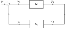
Consider the standard feedback closed-loop system $\Sigma_{1},\Sigma_{2}$ which is shown in Fig. 1. Assume that $\Sigma_{1}$ is output strictly passive, i.e. there exists a storage function $H_{1}$ such that $\dot{H}_{1}\leq u_{1}^{T}y_{1}-y_{1}\psi(y_{1})$ where $y_{1}\psi(y_{1})\geq 0$, and $\Sigma_{2}$ is passive, i.e. there exists a storage function $H_{2}$ such that $\dot{H}_{2}\leq u_{2}^{T}y_{2}.$ Then the states of $\Sigma_{1}$ converge to zero while states of $\Sigma_{2}$ remain bounded.

In order to use the above proposition, we shall modify right hand side of (21) in such a way that all the terms are represented by a regressor matrix and an unknown vector. Therefore, in the following, $Y\tilde{\Theta}\frac{Y_{a}\tilde{\theta}_{a}}{Y_{b}\hat{\theta}_{b}}$ and $\frac{Y_{b}\tilde{\theta}_{b}}{Y_{b}\hat{\theta}_{b}}Y_{c}\tilde{\theta}_{c}$ are changed accordingly. Assume that

$$\frac{Y_{b}\tilde{\theta}_{b}}{Y_{b}\hat{\theta}_{b}}Y_{c}\tilde{\theta}_{c}\triangleq\frac{Y_{c}Y_{\mu}}{Y_{b}\hat{\theta}_{b}}\tilde{\theta}_{\mu}$$

with,

$$\begin{array}[]{c}\leavevmode\resizebox{455.6629pt}{}{$Y_{\mu}=\begin{bmatrix}Y_{b}&0_{1\times k}&\dots&0_{1\times k}\\ 0_{1\times k}&Y_{b}&0_{1\times k}&\dots\\ \vdots&&\ddots&\vdots\\ 0_{1\times k}&\cdots&0_{1\times k}&Y_{b}\end{bmatrix}_{n\times p\cdot k},\tilde{\theta}_{\mu}=\begin{bmatrix}\Big{(}\prescript{}{1}{(\tilde{\theta}_{c}\tilde{\theta}_{b}^{T})}\Big{)}^{T}\\ \vdots\\ \Big{(}\prescript{}{p}{(\tilde{\theta}_{c}\tilde{\theta}_{b}^{T})}\Big{)}^{T}\end{bmatrix}$}\end{array}$$

and $\prescript{}{i}{(\tilde{\theta}_{c}\tilde{\theta}_{b}^{T})}$ is the $i$-th row of $\tilde{\theta}_{c}\tilde{\theta}_{b}^{T}$. Furthermore,

$$Y\tilde{\Theta}\frac{Y_{a}\tilde{\theta}_{a}}{Y_{b}\hat{\theta}_{b}}=\frac{YY_{\eta}}{Y_{b}\hat{\theta}_{b}}\tilde{\theta}_{\eta}$$

where,

$$\begin{array}[]{c}Y_{\eta}=\\ \leavevmode\resizebox{455.6629pt}{}{$\begin{bmatrix}\prescript{}{1}{(Y_{a})},...,\prescript{}{m}{(Y_{a})}&0_{1\times m.r}&\dots&0_{1\times m\cdot r}\\ 0_{1\times m\cdot r}&\prescript{}{1}{(Y_{a})},...,\prescript{}{m}{(Y_{a})}&&0_{1\times m\cdot r}\\ \vdots&&\ddots&\vdots\\ 0_{1\times m\cdot r}&\dots&&\prescript{}{1}{(Y_{a})},...,\prescript{}{m}{(Y_{a})}\end{bmatrix}_{l\times m\cdot r\cdot l}$}\end{array}$$

in which $\prescript{}{i}{(Y_{a})}$ is $i$-th row of $Y_{a}$, and

$$\begin{array}[]{c}\tilde{\theta}^{\prime}_{\eta}=\begin{bmatrix}\tilde{\Theta}_{1,1}\tilde{\theta}^{T}_{a}&\dots&\tilde{\Theta}_{1,m}\tilde{\theta}^{T}_{a}\\ \vdots&\ddots&\vdots\\ \tilde{\Theta}_{l,1}\tilde{\theta}^{T}_{a}&\dots&\tilde{\Theta}_{l,m}\tilde{\theta}^{T}_{a}\end{bmatrix}_{l\times m\cdot r},\tilde{\theta}_{\eta}=\begin{bmatrix}\prescript{}{1}{(\tilde{\theta}^{\prime}_{\eta})}^{T}\\ \vdots\\ \prescript{}{l}{(\tilde{\theta}^{\prime}_{\eta})}^{T}\end{bmatrix}_{m\cdot r\cdot l\times 1}\end{array}$$

where $\tilde{\Theta}_{i,j}$ is $(i,j)$-th element of $\tilde{\Theta}$. Therefore, (21) may be rewritten as follows:

$$\begin{array}[]{c}M\dot{S}+CS+KS=\\ \frac{Y\hat{\Theta}Y_{a}}{Y_{b}\hat{\theta}_{b}}\tilde{\theta}_{a}-\frac{YY_{\eta}}{Y_{b}\hat{\theta}_{b}}\tilde{\theta}_{\eta}+\frac{Y_{c}Y_{\mu}}{Y_{b}\hat{\theta}_{b}}\tilde{\theta}_{\mu}-\frac{Y_{c}\hat{\theta}_{c}Y_{b}}{Y_{b}\hat{\theta}_{b}}\tilde{\theta}_{b}\triangleq Y_{F}\tilde{\theta}_{F},\end{array}$$ (22)

where,

$$F=\begin{bmatrix}\frac{Y\hat{\Theta}Y_{a}}{Y_{b}\hat{\theta}_{b}}&-\frac{YY_{\eta}}{Y_{b}\hat{\theta}_{b}}&\frac{Y_{c}Y_{\mu}}{Y_{b}\hat{\theta}_{b}}&-\frac{Y_{c}\hat{\theta}_{c}Y_{b}}{Y_{b}\hat{\theta}_{b}}\end{bmatrix}$$

$$\tilde{\theta}_{F}=\begin{bmatrix}\tilde{\theta}_{a}\\ \tilde{\theta}_{\eta}\\ \tilde{\theta}_{\mu}\\ \tilde{\theta}_{b}\end{bmatrix}\in\mathbb{R}^{(r+m\cdot r\cdot l+p\cdot k+k)\times 1}.$$

Equation (22) may be considered as the system $\Sigma_{1}$ represented in Proposition 1. This system is output strictly passive with $H_{1}=\frac{1}{2}S^{T}MS$ as the storage function, because

$$\dot{H}\leq-\lambda_{min}\{K\}\|S\|^{2}+S^{T}u_{1}$$

with $u_{1}=Y_{F}\tilde{\theta}_{F},y_{1}=u_{2}=S$ and without external input (i.e. $v_{1}=0$). In order to apply Proposition 1, an adaptation law is required to be defined for $\tilde{\theta}_{F}$ such that $\Sigma_{2}$ becomes passive. For this means, the following dynamic is set for $\tilde{\theta}_{F}$

$$\dot{\hat{\theta}}_{F}=-\Lambda^{-1}Y^{T}_{F}S\hskip 42.67912pt\Lambda>0$$ (23)

which leads to the passivity of $\Sigma_{2}$, since

$$H_{2}=\frac{1}{2}\tilde{\theta}^{T}_{F}\Lambda\tilde{\theta}_{F}\to\dot{H}_{2}=-S^{T}Y_{F}\tilde{\theta}_{F}=u_{2}^{T}y_{2}.$$

Note that it is assumed that $\theta_{F}$ is constant. Let us state the following theorem on adaptive passivity based control of parallel robots with kinematics and dynamics uncertainties.

Theorem 1.

Consider a parallel robot with dynamic equation (1), control law (15) and adaptation law (23). The tracking error converges to zero in the presence of uncertainties in kinematics and dynamics parameters.

Proof.

The proof is obvious with respect to Proposition 1 and $\Sigma_{1},\Sigma_{2}$ defined above. However, a Lyapunov based proof is also presented here. Consider the following Lyapunov function candidate:

$$V=\frac{1}{2}S^{T}MS+\frac{1}{2}\tilde{\theta}^{T}_{F}\Lambda\tilde{\theta}_{F}.$$ (24)

then its time derivative becomes

$$\dot{V}\leq-S^{T}KS.$$

Invoking Lasalle-Yoshizawa Theorem [17, Theorem 8.4], it is easy to show that $S$ converges to zero, and hence, the convergence of $\tilde{X}$ is resulted from (10). ∎

Remark 1.

There may be a number of parameters in multiple unknown vectors that may not converge to their real values. However, this does not cause any problem for a suitable trajectory tracking.

Remark 2.

Singularity avoidance in construction and path planing is a necessary and important requirement in parallel robots [18]. Here, it is assumed that desired trajectory is inside its workspace far from singular space of the robot. By this means, the Jacobian matrix is always full rank, and therefore, its estimation is plausible. However, projection algorithm may be employed in order to ensures singularity avoidance as well as avoiding large variation in parameters and provides a faster and better transient response. Note that by this means, positive tension in the case of cable driven robots is ensured.

In the following lemma, invoking [1, Theorem 4.4.1], a projection algorithm based on gradient method is proposed.

Lemma 1.

Consider closed-loop system (22) with adaptation law (23). Assume that it is priori known that ${\theta}_{F}$ is absolutely in a compact subspace $\Omega$, i.e. ${\theta}_{F}\in\Omega$ where $\Omega$ is defined as $\Omega=\{{\theta}_{F}|g({\theta}_{F})\leq 0\}$ and $g({\theta}_{F})$ is known. The objective is to keep $\hat{\theta}_{F}$ in $\Omega$. If $\hat{\theta}_{F}$ is on the edge of $\Omega$ i.e. $\hat{\theta}_{F}\in\partial\Omega$, and $\dot{\hat{\theta}}_{F}^{T}\nabla g>0$, the following adaptation law is chosen

$$\dot{\hat{\theta}}_{F}=-\Lambda^{-1}\overline{\nabla g}Y_{F}^{T}S$$ (25)

where $\overline{\nabla g}$ is projection matrix

$$\overline{\nabla g}=I-\frac{(\nabla g)(\nabla g)^{T}}{||\nabla g||^{2}}.$$ (26)

This leads to $\hat{\theta}_{F}$ to remains in $\Omega$.

Proof.

If $\hat{\theta}_{F}$ is inside $\Omega$, adaptation law (23) is applied, and by this means, it remains in $\Omega$. Assume that ${\hat{\theta}_{F}}\in\partial\Omega$, hence the aim is to ensure that $\hat{\theta}_{F}$ always remains in $\Omega$. For this means, the direction of $\dot{\hat{\theta}}_{F}$ should not be directed toward outside of $\Omega$. In other words, dot product of $\dot{\hat{\theta}}_{F}$ and $\nabla g=\partial g/\partial\theta$ shall be non-positive. Therefore, if $(-\Lambda^{-1}Y^{T}_{F}S)^{T}\nabla g>0$, $\dot{\hat{\theta}}_{F}$ should be projected on the direction tangent to $\partial\Omega$. This is done using projection matrix (26) which results in adaptation law (25). Now consider Lyapunov candidate (24) whose time derivative is given as:

$$\dot{V}=-S^{T}KS+S^{T}Y_{F}\tilde{\theta}_{F}-\tilde{\theta}_{F}^{T}\overline{\nabla g}Y_{F}^{T}S.$$

By considering (26), $\dot{V}$ becomes

$$\dot{V}\leq-\lambda_{min}\{K\}\|S\|^{2}+\tilde{\theta}_{F}^{T}\frac{(\nabla g)(\nabla g)^{T}}{||\nabla g||^{2}}Y_{F}^{T}S.$$

Note that $\tilde{\theta}_{F}^{T}\nabla g\geq 0$, since direction of $\tilde{\theta}_{F}$ and $\nabla g$ are toward outside of $\Omega$. Therefore, the last term in the above inequality is negative. ∎

Notice that in most cases, exact derivation of $g(\theta_{F})$ is highly complicated. Hence, the acceptable bound for each element of unknown vector is considered and the simplest projection function, namely saturation is used, since it is applicable to any adaptive control law [19]. In other words, this is equivalent to define an absolute value function for every elements of unknown vectors. For example, Assume that $\alpha\in\mathbb{R}$ is an element of an unknown vector and it is known that $k_{1}\leq\alpha\leq k_{2}$. Define $g(\alpha)$ as

$$g(\alpha)=\left|\alpha-\frac{k_{1}+k_{2}}{2}\right|-\frac{k_{2}-k_{1}}{2}.$$

Now, one may find $\nabla g=\text{sign}(\alpha-\frac{k_{1}+k_{2}}{2})$ which leads to $\overline{\nabla g}=0$ and therefore, $\dot{\hat{\alpha}}=0$ when $\alpha$ is at the edge of $g(\alpha)\leq 0$.

Figure 2: Schematic of the 2–DOF RPR parallel robot.

IV Simulation Results

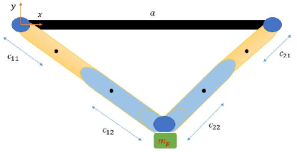
In this section, simulation results of proposed method on a 2–DOF RPR parallel robot is presented. The schematic of this robot is illustrated in Fig. 2. $X=[x,y]^{T}$ denotes position of end-effector, $I_{xi}$ is moment of inertial of $i$-th link, $m_{i1}$ and $m_{i2}$ are the mass of $i$-th cylinder and piston, respectively and $m_{p}$ denotes the mass of end-effector. The dynamic parameters and Jacobian matrix of the robot are

$$M =m_{p}I_{2}+\displaystyle\sum_{i=1}^{2}m_{i2}\hat{\lambda}_{i}\hat{\lambda}_{i}^{T}-\frac{1}{l_{i}^{2}}I_{xi}\hat{\lambda}_{i\times}^{2}-m_{ce}\hat{\lambda}_{i\times}^{2}$$

$$C =\displaystyle\sum_{i=1}^{2}-\frac{2}{l_{i}}m_{co}\dot{l}_{i}\hat{\lambda}_{ix}^{2}-\frac{1}{l_{i}^{2}}m_{i2}c_{i2}\hat{\lambda}_{i}\dot{X}^{T}\hat{\lambda}_{ix}^{2}$$

$$G =\bigg{(}m_{p}+\displaystyle\sum_{i=1}^{2}m_{ge}\hat{\lambda}_{ix}^{2}-m_{i2}\hat{\lambda}_{i}\hat{\lambda}_{i}^{T}\bigg{)}\begin{bmatrix}0\\ g\end{bmatrix}$$

$$J =-\begin{bmatrix}\frac{x}{l_{1}}&\frac{y}{l_{1}}\\ \frac{x-a}{l_{2}}&\frac{y}{l_{2}}\end{bmatrix},\hat{\lambda}_{1}=\begin{bmatrix}\frac{x}{l_{1}}\\ \frac{y}{l_{1}}\end{bmatrix},\hat{\lambda}_{2}=\begin{bmatrix}\frac{x-a}{l_{2}}\\ \frac{y}{l_{2}}\end{bmatrix}$$

with

$$l_{1}^{2} =x^{2}+y^{2},\quad l_{2}^{2}=(x-a)^{2}+y^{2},\quad\dot{l}_{i}=J_{i,1}\dot{x}+J_{i,2}\dot{y}$$

$$m_{ce} =\displaystyle\sum_{i=1}^{2}\frac{1}{l_{i}^{2}}\big{(}m_{i1}c_{i1}^{2}+m_{i2}c_{i2}^{2}\big{)}$$

$$m_{co} =\frac{1}{l_{i}}m_{i2}c_{i2}-\frac{1}{l_{i}^{2}}(I_{xi}+l_{i}^{2}m_{ce})$$

$$m_{ge} =\frac{1}{l_{i}}\Big{(}m_{i1}c_{i1}+m_{i2}(l_{i}-c_{i2})\Big{)}.$$

TABLE I: Parameters of 2RPR robot.

	$m_{i1}$	$m_{i2}$	$c_{i1}$	$c_{i2}$	$I_{xi}$
$i=1$	1	1	0.5	0.5	0.1
$i=2$	1	1	0.5	0.5	0.1

The parameters of the robot are shown in Table I. The mass of end-effector is considered equal to 2Kg. All of the regressors are represented in Appendix.

In order to evaluate performance of proposed method in Theorem 1, a simulation with adaptive robust controller proposed in [15] is considered. The parameters of the robot are perturbed by 25%. The gains of controllers are chosen as

$$\Gamma=2I,\qquad K=3I,\qquad\Lambda=5I.$$

Simulation results are illustrated in Fig. 3. Configuration variables of the robot converge to desired values in both methods. However, the control signal with adaptive robust method has an undesirable chattering which is not practically acceptable. Note that as indicated in [15], it is possible to avoid chattering with the expense of loosening the asymptotic stability to UUB tracking error.

(a) Simulation results of the proposed method.

(b) Simulation results of adaptive robust controller proposed by [15].

Figure 3: Tracking error converges to zero with both method while chattering in control law is destructive inevitable part of adaptive robust controller.

V Experimental Results

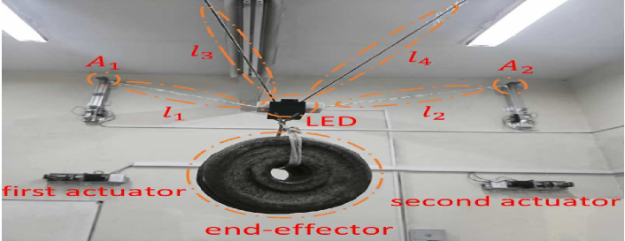
In order to verify the performance of the proposed method in experiment, a 3–DOF suspended Cable Driven Robot (CDR) is considered. The schematic of the robot is illustrated in Fig. 4. End-effector is suspended from anchor points by cables which are controlled by motors. All of the anchor points are in the same height. The robot has three translational degrees of freedom with four actuated cables which are driven by motors through pulleys.

Figure 4: Schematic of the suspended robot with four cables. All of the anchor points are at the same height. Center of coordinates is located in the middle of $A_{1}-A_{2}-A_{3}-A_{4}$ rectangle with zero height.

Kinematics formulation of this robot is given by

$$l_{i}^{2}=(x-x_{Ai})^{2}+(y-y_{Ai})^{2}+(z-z_{Ai})^{2}\quad i=1,...,4$$ (27)

where, $X=[x,y,z]^{T}$ is the position of end-effector and $x_{Ai},y_{Ai},z_{Ai}$ are the uncertain kinematic parameters that determine the cable anchor points. Dynamic matrices of the robot with the assumption of massless and infinitely stiff cables are as follows

$$M=\begin{bmatrix}m&0&0\\ 0&m&0\\ 0&0&m\end{bmatrix}\quad C=0_{3\times 3}\quad G=\begin{bmatrix}0\\ 0\\ mg\end{bmatrix}$$ (28)

where $m$ is the mass of end-effector.

Since the proposed method is also applicable to redundantly actuated parallel robots, the experiment is designed such that the method is applied to redundant CDR. The Jacobian matrix may be rearranged into the following form:

$$\begin{array}[]{c}J^{T}=-\begin{bmatrix}x-x_{A1}&x-x_{A2}&x-x_{A3}&x-x_{A4}\\ y-y_{A1}&y-y_{A2}&y-y_{A3}&y-y_{A4}\\ z-z_{A1}&z-z_{A2}&z-z_{A3}&z-z_{A4}\end{bmatrix}\\ \begin{bmatrix}\frac{1}{l_{1}}&0&0&0\\ 0&\frac{1}{l_{2}}&0&0\\ 0&0&\frac{1}{l_{3}}&0\\ 0&0&0&\frac{1}{l_{4}}\end{bmatrix}.\end{array}$$ (29)

Thus, Jacobian matrix is expressed in the form $J^{T}=J^{T}_{new}(X)L^{-1}$. Now it is possible to express $J_{new}^{T}$ in regressor form

$$\begin{array}[]{c}J_{new}^{T}=\begin{bmatrix}x&x&x&x\\ y&y&y&y\\ z&z&z&z\end{bmatrix}+\begin{bmatrix}-1&0&0\\ 0&-1&0\\ 0&0&-1\end{bmatrix}\times\\ \begin{bmatrix}x_{A1}&x_{A2}&x_{A3}&x_{A4}\\ y_{A1}&y_{A2}&y_{A3}&y_{A4}\\ z_{A1}&z_{A2}&z_{A3}&z_{A4}\end{bmatrix}=\begin{bmatrix}x&x&x&x\\ y&y&y&y\\ z&z&z&z\end{bmatrix}\par+Y\Theta.\end{array}$$ (30)

$Y_{a}\theta_{a},Y_{b}\theta_{b}$ and $Y_{c}\theta_{c}$ are determined in Appendix.

(a) Various components of ARAS suspended cable robot

(b) The prototype of a stereo vision system, which is attached to the ceiling of laboratory in the geometrical center of the top of the workspace.

Figure 5: ARAS suspended cable driven robot

(a) Path of the robot with adaptive and non-adaptive controllers. In contrast to non-adaptive response which is based on calibrated model, the path with adaptive controller is almost matched with the desired path after a transient response.

(b) Tracking error of $x$ in centimeter. Maximum remaining error with adaptive controller is less than 0.5cm which shows superiority of proposed method compared to the method based on calibration.

(c) Tracking error of $y$ in centimeter. Maximum remaining error with adaptive controller is about 0.5cm which shows superiority of proposed method compared to the method based on calibration.

(d) Tracking error of $z$ in centimeter. Maximum remaining error with adaptive controller is about 0.25cm which shows great response of proposed methods compared to the method based on calibration.

Figure 6: Experiment results of the adaptive and non-adaptive controllers on a 3–DOF CDR. Tracking errors with proposed controller is smaller than the non-adaptive controller based on calibrated model.

Figure 7: Control efforts of adaptive and non-adaptive controllers in the experiment. The reason for oscillation at the initial moments are fluctuations in cables. The control laws with proposed method have more small fluctuations due to adaptation laws.

$$\prescript{}{1}{Y^{\prime}}_{c}=[x^{2}\ddot{X}_{r1}/l_{1}^{2}+xy\ddot{X}_{r2}/l_{1}^{2}+\ddot{X}_{r1}x^{2}/l_{2}^{2}+xy\ddot{X}_{r2}/l_{2}^{2},+y^{2}\ddot{X}_{r1}/l_{1}^{4}-xy\ddot{X}_{r2}/l_{1}^{4}+y^{2}\ddot{X}_{r1}/l_{2}^{4}-xy\ddot{X}_{r2}/l_{2}^{4}-2xy^{2}\dot{X}_{r1}/l_{1}^{6}$$

$$+xy^{2}\dot{x}\dot{X}_{r1}/l_{1}^{5}-x^{2}y\dot{y}\dot{X}_{r1}/l_{1}^{5}-x^{2}y\dot{x}\dot{X}_{r2}/l_{1}^{5}+x^{3}\dot{y}\dot{X}_{r2}/l_{1}^{5}+xy^{2}\dot{x}\dot{X}_{r1}/l_{2}^{5}-x^{2}y\dot{y}\dot{X}_{r1}/l_{2}^{5}-x^{2}y\dot{x}\dot{X}_{r2}/l_{2}^{5}+x^{3}\dot{y}\dot{X}_{r2}/l_{2}^{5},\ddot{X}_{r1},$$

$$-2x\ddot{X}_{r1}/l_{2}^{2}-y\ddot{X}_{r2}/l_{2}^{2},+y\ddot{X}_{r2}/l_{2}^{4}+2y^{2}\dot{X}_{r1}/l_{2}^{6}-4xy\dot{X}_{r2}/l_{2}^{6},+2y\ddot{X}_{r2}/l_{2}^{4}+4y^{2}\dot{X}_{r1}/l_{2}^{6}-8xy\dot{X}_{r2}/l_{2}^{6},-2y^{2}\dot{X}_{r1}/l_{2}^{5}$$

$$+4xy\dot{X}_{r2}/l_{2}^{5}-y^{2}\dot{x}\dot{X}_{r1}/l_{2}^{5}+2xy\dot{y}\dot{X}_{r1}/l_{2}^{5}+2xy\dot{x}\dot{X}_{r2}/l_{2}^{5}+3x^{2}\dot{y}\dot{X}_{r2}/l_{2}^{5},\ddot{X}_{r1}/l_{2}^{2},2y\dot{X}_{r2}/l_{2}^{6},4y\dot{X}_{r2}/l_{2}^{6},-2y\dot{X}_{r2}/l_{2}^{5}$$

$$-y\dot{y}\dot{X}_{r1}/l_{2}^{5}-y\dot{x}\dot{X}_{r2}/l_{2}^{5}+3x\dot{y}\dot{X}_{r2}/l_{2}^{5},0,0,0,-\dot{y}\dot{X}_{r2}/l_{2}^{5}],$$

$$\prescript{}{2}{Y^{\prime}}_{c}=[xy\ddot{X}_{r1}/l_{1}^{2}+y^{2}\ddot{X}_{r2}/l_{1}^{2}+xy\ddot{X}_{r1}/l_{2}^{2}+y^{2}\ddot{X}_{r2}/l_{2}^{2}+gx^{2}/l_{1}^{2}+gy^{2}/l_{1}^{2}+gx^{2}/l_{2}^{2}+gy^{2}/l_{2}^{2},-xy\ddot{X}_{r1}/l_{1}^{4}+x^{2}\ddot{X}_{r2}/l_{1}^{4}$$

$$+4x^{2}y\dot{X}_{r1}/l_{2}^{6}+4xy^{2}\dot{X}_{r1}/l_{2}^{6}-4x^{3}\dot{X}_{r2}/l_{2}^{6}-4x^{2}y\dot{X}_{r2}/l_{2}^{6},-2x^{2}y\dot{X}_{r1}/l_{1}^{5}-2xy^{2}\dot{X}_{r1}/l_{1}^{5}+2x^{3}\dot{X}_{r2}/l_{1}^{5}+2x^{2}y\dot{X}_{r2}/l_{1}^{5}$$

$$-2x^{2}y\dot{X}_{r1}/l_{2}^{5}-2xy^{2}\dot{X}_{r1}/l_{2}^{5}+2x^{3}\dot{X}_{r2}/l_{2}^{5}+2x^{2}y\dot{X}_{r2}/l_{2}^{5}+y^{3}\dot{x}\dot{X}_{r1}/l_{1}^{5}-xy^{2}\dot{y}\dot{X}_{r1}/l_{1}^{5}-xy^{2}\dot{x}\dot{X}_{r2}/l_{1}^{5}+x^{2}y\dot{y}\dot{X}_{r2}/l_{1}^{5}$$

$$+y^{3}\dot{x}\dot{X}_{r1}/l_{2}^{5}-x^{2}y\dot{y}\dot{X}_{r1}/l_{2}^{5}-xy^{2}\dot{x}\dot{X}_{r2}/l_{2}^{5}-x^{2}y\dot{y}\dot{X}_{r2}/l_{2}^{5},\ddot{X}_{r2}+g,-y\ddot{X}_{1}/l_{2}^{2}-g2x/l_{2}^{2},y\ddot{X}_{1}/l_{2}^{4}-2x\ddot{X}_{2}/l_{2}^{4}-4xy\dot{X}_{1}/l_{2}^{6}$$

$$-2y^{2}\dot{X}_{1}/l_{2}^{6}-6x^{2}\dot{X}_{2}/l_{2}^{6}+4xy\dot{X}_{2}/l_{2}^{6},2y\ddot{X}_{1}/l_{2}^{4}-4x\ddot{X}_{2}/l_{2}^{4}-8xy\dot{X}_{1}/l_{2}^{6}-4y^{2}\dot{X}_{1}/l_{2}^{6}-12x^{2}\dot{X}_{2}/l_{2}^{6}+8xy\dot{X}_{2}/l_{2}^{6},4xy\dot{X}_{r1}/l_{2}^{5}$$

$$+2y^{2}\dot{X}_{r1}/l_{2}^{5}+6x^{2}\dot{X}_{r2}/l_{2}^{5}-4xy\dot{X}_{r2}/l_{2}^{5}+y^{2}\dot{y}\dot{X}_{r1}/l_{2}^{5}+y^{2}\dot{x}\dot{X}_{r2}/l_{2}^{5}+2xy\dot{y}\dot{X}_{r2}/l_{2}^{5},g/l_{2}^{2},\ddot{X}_{r2}/l_{2}^{4}+2y\dot{X}_{r1}/l_{2}^{6}+6x\dot{X}_{r2}/l_{2}^{6},$$

$$2g/l_{2}^{2},2\ddot{X}_{r2}/l_{2}^{4}+4y\dot{X}_{r1}/l_{2}^{6}+12x\dot{X}_{r2}/l_{2}^{6},-2y\dot{X}_{r1}/l_{2}^{5}-6x\dot{X}_{r2}/l_{2}^{5}+2y\dot{X}_{r2}/l_{2}^{5}-y\dot{y}\dot{X}_{r2}/l_{2}^{5},0,2\dot{X}_{r2}/l_{2}^{5},4\dot{X}_{r2}/l_{2}^{5},2\dot{X}_{r2}/l_{2}^{5}].$$ (31)

$$\hskip 241.84842pt\mathclap{\rule{483.69684pt}{0.4pt}}$$

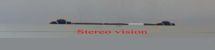
In order to measure the length of cables, the motor rotation angles are measured by incremental encoders. Hence, the current length of cables are available by knowing initial length of the them. A 100 frame per second stereo vision camera with $640\times 480$ resolution is utilized to measure position of the LED lamp as the position of the end-effector. More information about the experimental setup is given in [11]. Fig. 5 shows different parts of ARAS cable driven suspended robot.

The mass of end-effector is equal to 4.5KG and coordinates of cable anchor points are obtained by calibration as:

$$\begin{split}&x_{A1}=-x_{A2}=x_{A3}=-x_{A4}=\frac{b}{2}=\frac{3.56}{2}\\ &y_{A1}=y_{A2}=-y_{A3}=-y_{A4}=\frac{a}{2}=\frac{7.05}{2}\\ &z_{A1}=z_{A2}=z_{A3}=z_{A4}=h=4.26\end{split}$$ (32)

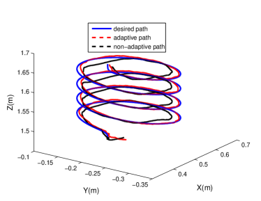
The spring-like desired trajectory is expressed in SI unit systems, as follows:

$$\begin{cases}x_{d}(t)=0.48-0.1\cos(\frac{2\pi}{5}t)\\ y_{d}(t)=-0.22+0.1\sin(\frac{2\pi}{5}t)\\ z_{d}(t)=1.5+0.0075t\end{cases}$$ (33)

The center and diameter of the trajectory are chosen in such a way that the robot is inside its workspace away from its singular points, and well-measured by the stereo camera. The adaptive passivity based method parameters which is applied to redundant case are set to:

$$\Gamma=20I,\qquad K=10I,\qquad\Lambda=5I.$$

The initial position of the robot is:

$$\begin{bmatrix}x_{0}\\ y_{0}\\ z_{0}\end{bmatrix}=\begin{bmatrix}0.43\\ -0.28\\ 1.5\end{bmatrix}.$$

Notice that in contrast to all previous works on ARAS CDR, in this work the initial position of the robot is not on the trajectory, i.e. $\tilde{X}$ is not zero at $t=0$. Note that such sudden motion request in cable driven robots may lead to longitudinal and transverse oscillations in cables which may cause instabilities in the robot. This extreme scenario is tested on the robot with suitable controller performance.

The upper bound of perturbation for dynamic and kinematic parameters is set to $10\%$. In order to examine the effect of the projection algorithm, a saturation function is used as a simple appropriate projection for the case of passivity based method. By this means, estimated parameters are saturated within the $\pm 15\%$ bounds. For the sake of comparison, and in order to analyze the performance of proposed methods, a non-adaptive controller is also implemented in practice. The control law is as what given in (12) with the parameters obtained from calibration. This is considered, since a calibrated model is not match exactly with nominal model of a robot. Note that a high gain controller was also implemented on the robot, whose results are not reported in this paper, since it led to instability due to the high oscillations in cables.

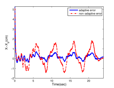
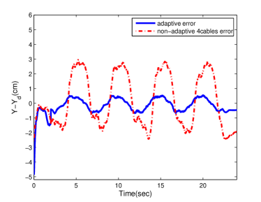
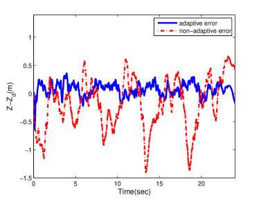
The experimental results are illustrated in Fig. 6 and Fig. 7. Performance of the controllers are depicted in Fig. 6. As it is seen in Fig. 6(a), the traversed path with adaptive controller suitably tracks the desired path with a short transient error. However, non-adaptive controller is not that precise, and leads to an apparent error throughout the path. In order to compare the results more clearly, the tracking errors are shown in Fig. 6(b), 6(c) and 6(d).

Note that the tracking error illustrated in these figures are in centimeters. The results show the desirable performance of the proposed method in comparison to non-adaptive controller based on the calibrated model. The response of the system is affected by the oscillations of cables at initial transient due to an initial error between the trajectory and position of the robot. After this period, fluctuations are suitably damped and thus, the robot has almost a repetitive response.

In Fig. 6(b), the tracking error in $X$ direction is less than $0.5$cm with adaptive controller while with the non-adaptive controller, it is about 2cm. The tracking errors in $Y$ and $Z$ directions are about 0.5cm and 0.25cm for proposed method and 3cm and 1.5cm with the non-adaptive controller, respectively. This shows superiority of the proposed methods compared to that of current available method, since the response is improved and bounds of the errors are decreased. Notice that the reason why error in $Y$ direction is almost double of that in $X$ direction is the distance between anchor points proposed in (32). Recall that in the case of non-adaptive controller, the kinematic and dynamic parameters are obtained based on a time consuming calibration. Indeed, if the parameters were unknown, a worse response or even instability, would be happen. Note that the non-vanishing error may be caused by a simple dynamic model assigned to the robot and dynamics of the actuators.

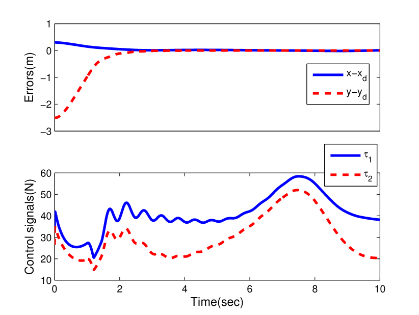
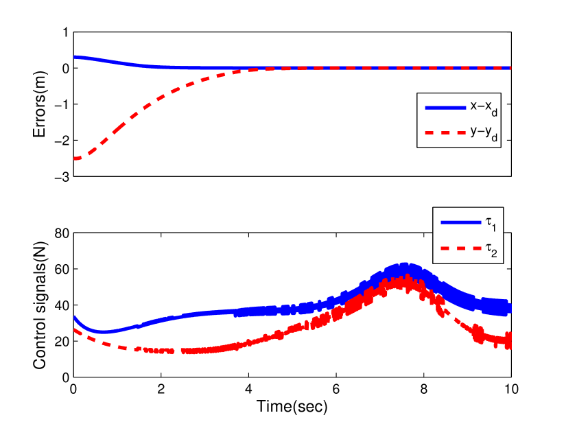
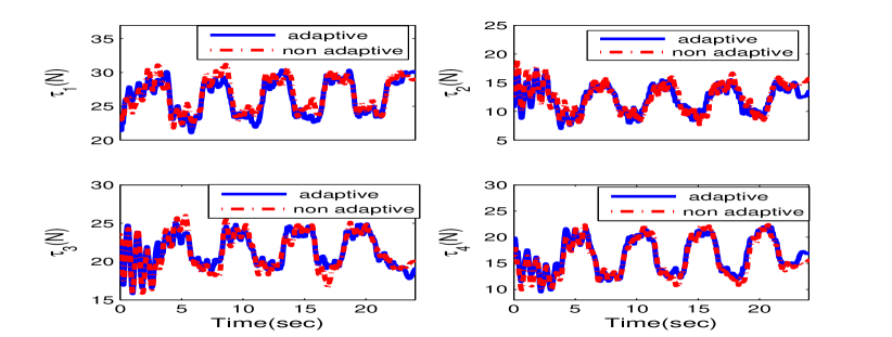
Fig. 7 shows control efforts for adaptive and non-adaptive controllers in experiments. As it is seen in this figure, some oscillations are observed at the initial moments. The main reason for such oscillations are the oscillations caused in the cables, because of its elasticity, while the reason why control laws with proposed method have smaller oscillations is the adaptation law. Note that all control signals are positive, since as explained in Remark 2, the desired trajectory is within the feasible workspace of the robot as well as using the projection algorithm, it is ensured that adapted parameters can not exceed from a specified bound. Finally as it is depicted in this figure, the control efforts needed in the proposed adaptive controller are almost similar to that of non-adaptive controller, despite their suitable tracking performance.

$$\prescript{}{1}{Y}_{a}=[-2z^{2}\ddot{X}_{r1}-2xz(\ddot{X}_{r3}+g),2z^{2}\big{(}\prescript{}{1}{K}S\big{)}+2xz\big{(}\prescript{}{3}{K}S\big{)},4z\ddot{X}_{r1}+2x(\ddot{X}_{r3}+g),-4z\big{(}\prescript{}{1}{K}S\big{)}-2x\big{(}\prescript{}{3}{K}S\big{)},-2\ddot{X}_{r1},$$

$$2\leavevmode\resizebox{429.28616pt}{}{$\big{(}\prescript{}{1}{K}S\big{)},-2z^{2}\ddot{X}_{r2}+yz(\ddot{X}_{r3}+g),2z^{2}\big{(}\prescript{}{2}{K}S\big{)}-yz\big{(}\prescript{}{3}{K}S\big{)},4z\ddot{X}_{r2}-y(\ddot{X}_{r3}+g),-4z\big{(}\prescript{}{2}{K}S\big{)}+y\big{(}\prescript{}{3}{K}S\big{)}-2\ddot{X}_{r2},2\big{(}\prescript{}{2}{K}S\big{)},$}$$

$$x-2y^{2}(\ddot{X}_{r3}+g),2y^{2}\big{(}\prescript{}{3}{K}S\big{)},12z(\ddot{X}_{r3}+g),-12z\big{(}\prescript{}{3}{K}S\big{)},-4(\ddot{X}_{r3}+g),4\big{(}\prescript{}{3}{K}S\big{)}],$$

$$\prescript{}{2}{Y}_{a}=[2z^{2}\ddot{X}_{r1}+2xz(\ddot{X}_{r3}+g),-2z^{2}\big{(}\prescript{}{1}{K}S\big{)}-2xz\big{(}\prescript{}{3}{K}S\big{)},v4z\big{(}\prescript{}{1}{K}S\big{)}+2x\big{(}\prescript{}{3}{K}S\big{)},-4z\ddot{X}_{r1}-2x(\ddot{X}_{r3}+g),2\ddot{X}_{r1},$$

$$-2y^{2}(\ddot{X}_{r3}+g),2y^{2}\big{(}\prescript{}{3}{K}S\big{)},12z(\ddot{X}_{r3}+g),-12z\big{(}\prescript{}{3}{K}S\big{)},-4(\ddot{X}_{r3}+g),4\big{(}\prescript{}{3}{K}S\big{)}],$$

$$22z^{2}\ddot{X}_{r2}+yz(\ddot{X}_{r3}+g),-2z^{2}\big{(}\prescript{}{2}{K}S\big{)}+yz\big{(}\prescript{}{3}{K}S\big{)},-4z\ddot{X}_{r2}+y(\ddot{X}_{r3}+g),4z\big{(}\prescript{}{2}{K}S\big{)}-y\big{(}\prescript{}{3}{K}S\big{)},2\ddot{X}_{r2},-2\big{(}\prescript{}{2}{K}S\big{)},(4x^{2}z$$

$$+4z^{3})(\ddot{X}_{r3}+g),-(4x^{2}z+4z^{3})\big{(}\prescript{}{3}{K}S\big{)},-(4x^{2}+12z^{2})(\ddot{X}_{r3}+g),(4x^{2}+12z^{2})\big{(}\prescript{}{3}{K}S\big{)},2y^{2}z(\ddot{X}_{r3}+g),-2y^{2}z\big{(}\prescript{}{3}{K}S\big{)},$$

$$-2y^{2}(\ddot{X}_{r3}+g),2y^{2}\big{(}\prescript{}{3}{K}S\big{)},12z(\ddot{X}_{r3}+g),-12z\big{(}\prescript{}{3}{K}S\big{)},-4(\ddot{X}_{r3}+g),4\big{(}\prescript{}{3}{K}S\big{)}],$$

$$\prescript{}{4}{Y}_{a}=[2z^{2}\ddot{X}_{r1}+2xz(\ddot{X}_{r3}+g),-2z^{2}\big{(}\prescript{}{1}{K}S\big{)}-2xz\big{(}\prescript{}{3}{K}S\big{)},-4z\ddot{X}_{r1}-2x(\ddot{X}_{r3}+g),4z\big{(}\prescript{}{1}{K}S\big{)}+2x\big{(}\prescript{}{3}{K}S\big{)},2\ddot{X}_{r1},$$

$$-2y^{2}(\ddot{X}_{r3}+g),2y^{2}\big{(}\prescript{}{3}{K}S\big{)},12z(\ddot{X}_{r3}+g),-12z\big{(}\prescript{}{3}{K}S\big{)},-4(\ddot{X}_{r3}+g),4\big{(}\prescript{}{3}{K}S\big{)}].$$ (34)

$$\hskip 241.84842pt\mathclap{\rule{483.69684pt}{0.4pt}}$$

VI Conclusions and Prospect Research

This paper focused on the design of adaptive tracking controller for parallel robots with dynamic and kinematic uncertainties. A novel expression for inverse of Jacobian matrix in regressor form was proposed, a methods based on passivity was introduced and adaptation law for unknown parameters was elicited. By this means, it was proved that the tracking error of the robot converges asymptotically to zero in the presence of kinematics, Jacobian and dynamic uncertainties. The performance of the controller was verified through simulation and experiment, and it has been shown that in comparison to available methods, the response is improved, while the effect of projection in singularity avoidance was highlighted. Since the research on the control of parallel robots in presence of kinematic and dynamic uncertainties is developing, future research may be devoted to decoupling the adaptation laws for kinematic and dynamic parameters in order to reduce the number of adapting parameters. Extension of the proposed method to the case of serial robots is also underway.

Regressor Forms of 2RPR robot

Jacobian matrix can be represented as:

$$J^{T} =\begin{bmatrix}\frac{x}{l_{1}}&\frac{x-a}{l_{2}}\\ \frac{y}{l_{1}}&\frac{y}{l_{2}}\end{bmatrix}=\begin{bmatrix}x&x-a\\ y&y\end{bmatrix}\begin{bmatrix}\frac{1}{l_{1}}&0\\ 0&\frac{1}{l_{2}}\end{bmatrix}=J_{new}^{T}L^{-1}$$

$$J_{new}^{T}=\begin{bmatrix}x&x\\ y&y\end{bmatrix}+\begin{bmatrix}0&-1\\ 0&0\end{bmatrix}a=\begin{bmatrix}x&x\\ y&y\end{bmatrix}+Y\Theta$$

$$T=ay=Y_{b}\theta_{b}.$$

Dynamic parameters of the system can be expressed by a regressor as follows

$$Y_{c}\theta_{c}=-KS+Y^{\prime}_{C}\theta^{\prime}_{c},$$

where $Y_{c}$ is proposed in (31) and $\theta^{\prime}_{c}$ is:

$$\theta^{\prime}_{c}=[m,I,mc^{2},mc,m_{p},ma,Ia,mc^{2}a,mca,ma^{2},Ia^{2},mc^{2}a^{2},$$

$$mca^{2},ma^{3},Ia^{3},mc^{2}a^{3},mca^{3}]^{T}\in\mathbb{R}^{17}.$$

$Y_{a}\theta_{a}$ proposed in (16) is obtained as follows

$$Y_{a}=[R_{1}Y_{c}\vdots 0_{4\times 2}]+[0_{4\times 2}\vdots Y_{c}],\quad R_{1}:=\begin{bmatrix}y&-x\\ -y&x\end{bmatrix},$$

$$\theta_{a}=[\theta_{c},a^{4}m,a^{4}I,a^{4}mc^{2},a^{4}mc]^{T}\in\mathbb{R}^{21}.$$

Regressor Forms of Redundant CDR

Consider, $a,b$ and $h$ as illustrated in Fig. 4 and presented in (32). Matrix $R$ proposed in (13) is

$Y_{a}$ is proposed in (34) and $\theta_{a}$ is given by

$$\begin{split}&\theta_{a}=[a^{2}bm,a^{2}b,a^{2}bhm,a^{2}bh,a^{2}bh^{2}m,a^{2}bh^{2},ab^{2}m,ab^{2},\\ &ab^{2}hm,ab^{2}h,ab^{2}h^{2}m,ab^{2}h^{2},a^{2}m,a^{2},a^{2}hm,a^{2}h,b^{2}m,b^{2},\\ &b^{2}hm,b^{2}h,a^{2}h^{2}m,a^{2}h^{2},a^{2}h^{3}m,a^{2}h^{3}]^{T}.\end{split}$$

The determinant $T=Y_{b}\theta_{b}$ is

$$\begin{split}&Y_{b}=[4z^{2},-8z,4,-128(x^{2}yz^{2}+xy^{2}z^{2}),256(x^{2}yz^{2}\\ &+xy^{2}z^{2})+128xyz^{2},-128(x^{2}yz^{2}+xy^{2}z^{2}),256xy],\end{split}$$

$$\theta_{b}=[a^{2}b^{2},a^{2}b^{2}h,a^{2}b^{2}h^{2},h,h^{2},h^{3},h^{4}]^{T}.$$

$Y_{c}\theta_{c}$ is given as

$$\begin{array}[]{c}M\ddot{X}_{r}+C\dot{X}_{r}+G-KS=-KS\\ +\left(\ddot{X}_{r}+\begin{bmatrix}0\\ 0\\ g\end{bmatrix}\right)m=-KS+Y_{c}\theta_{c}.\end{array}$$ (35)

Construction of $Y_{F}\theta_{F}$ is a bit lengthy but straightforward.

References

• [1] P. A. Ioannou and J. Sun, Robust adaptive control. Courier Corporation, 2012.
• [2] R. Ortega and M. W. Spong, “Adaptive motion control of rigid robots: A tutorial,” Automatica, vol. 25, no. 6, pp. 877–888, 1989.
• [3] Y. Xia, K. Xu, Y. Li, G. Xu, and X. Xiang, “Modeling and three-layer adaptive diving control of a cable-driven underwater parallel platform,” IEEE Access, vol. 6, pp. 24016–24034, 2018.
• [4] J.-J. E. Slotine and W. Li, “On the adaptive control of robot manipulators,” The international journal of robotics research, vol. 6, no. 3, pp. 49–59, 1987.
• [5] C.-C. Cheah, C. Liu, and J.-J. E. Slotine, “Approximate jacobian adaptive control for robot manipulators,” in Robotics and Automation, 2004. Proceedings. ICRA’04. 2004 IEEE International Conference on, vol. 3, pp. 3075–3080, IEEE, 2004.
• [6] C.-C. Cheah, C. Liu, and J.-J. E. Slotine, “Adaptive tracking control for robots with unknown kinematic and dynamic properties,” The International Journal of Robotics Research, vol. 25, no. 3, pp. 283–296, 2006.
• [7] H. Wang, “Adaptive control of robot manipulators with uncertain kinematics and dynamics,” IEEE Transactions on Automatic Control, vol. 62, no. 2, pp. 948–954, 2016.
• [8] H. D. Taghirad, Parallel robots: mechanics and control. CRC press, 2013.
• [9] M. R. J. Harandi and H. D. Taghirad, “Motion control of an underactuated parallel robot with first order nonholonomic constraint,” in 2017 5th RSI International Conference on Robotics and Mechatronics (ICRoM), pp. 582–587, IEEE, 2017.
• [10] S.-R. Oh and S. K. Agrawal, “A reference governor-based controller for a cable robot under input constraints,” IEEE transactions on control systems technology, vol. 13, no. 4, pp. 639–645, 2005.
• [11] S. Khalilpour, R. Khorrambakht, H. Taghirad, and P. Cardou, “Robust cascade control of a deployable cable-driven robot,” Mechanical Systems and Signal Processing, vol. 127, pp. 513–530, 2019.
• [12] G. Chen, L. Kong, Q. Li, H. Wang, and Z. Lin, “Complete, minimal and continuous error models for the kinematic calibration of parallel manipulators based on poe formula,” Mechanism and Machine Theory, vol. 121, pp. 844–856, 2018.
• [13] G. Meunier, B. Boulet, and M. Nahon, “Control of an overactuated cable-driven parallel mechanism for a radio telescope application,” IEEE transactions on control systems technology, vol. 17, no. 5, pp. 1043–1054, 2009.
• [14] R. Babaghasabha, M. A. Khosravi, and H. D. Taghirad, “Adaptive control of kntu planar cable-driven parallel robot with uncertainties in dynamic and kinematic parameters,” in Cable-Driven Parallel Robots, pp. 145–159, Springer, 2015.
• [15] R. Babaghasabha, M. A. Khosravi, and H. D. Taghirad, “Adaptive robust control of fully-constrained cable driven parallel robots,” Mechatronics, vol. 25, pp. 27–36, 2015.
• [16] A. J. van der Schaft and A. Van Der Schaft, L2-gain and passivity techniques in nonlinear control, vol. 3. Springer, 2017.
• [17] H. K. Khalil and J. Grizzle, Nonlinear systems, vol. 3. Prentice hall Upper Saddle River, NJ, 2002.
• [18] C. Gosselin and L.-T. Schreiber, “Kinematically redundant spatial parallel mechanisms for singularity avoidance and large orientational workspace,” IEEE Transactions on Robotics, vol. 32, no. 2, pp. 286–300, 2016.
• [19] W. E. Dixon, “Adaptive regulation of amplitude limited robot manipulators with uncertain kinematics and dynamics,” IEEE Transactions on Automatic Control, vol. 52, no. 3, pp. 488–493, 2007.