Fully-Discrete Explicit Locally Entropy-Stable Schemes for the Compressible Euler and Navier–Stokes Equations

Abstract

Recently, relaxation methods have been developed to guarantee the preservation of a single global functional of the solution of an ordinary differential equation. Here, we generalize this approach to guarantee local entropy inequalities for finitely many convex functionals (entropies) and apply the resulting methods to the compressible Euler and Navier–Stokes equations. Based on the unstructured $hp$-adaptive SSDC framework of entropy conservative or dissipative semidiscretizations using summation-by-parts and simultaneous-approximation-term operators, we develop the first discretizations for compressible computational fluid dynamics that are primary conservative, locally entropy stable in the fully discrete sense under a usual CFL condition, explicit except for the parallelizable solution of a single scalar equation per element, and arbitrarily high-order accurate in space and time. We demonstrate the accuracy and the robustness of the fully-discrete explicit locally entropy-stable solver for a set of test cases of increasing complexity.

AMS subject classification. 65M12, 65M70, 65L06, 65L20, 65P10, 76M10, 76M20, 76M22, 76N99

1 Introduction

Consider an ordinary differential equation (ODE)

$$u^{\prime}(t)=f(u(t))\quad u(0)=u^{0},$$ (1.1)

in a Banach space. Throughout the paper, we use upper indices to denote the index of the corresponding time step. In various applications in science and engineering, there are often smooth energy/entropy/Lyapunov functionals, $\eta$, whose evolution in time is important, e.g., to provide some stability estimates [19, Chapter 5]. Often, the time derivative of $\eta$ satisfies

$$\dfrac{\operatorname{d\!}{}}{\operatorname{d\!}{t}}\eta(u(t))\leq 0$$ (1.2a)

for all solutions $$u$$ of (1.1), i.e.,

$$\forall u\colon\quad\eta^{\prime}(u)f(u)\leq 0.$$ (1.2b)

Problem (1.1) is said to be dissipative if (1.2) holds and conservative if there is an equality in (1.2). However, the relaxation approach described in the following is not limited to conservative or dissipative problems. Instead, this approach can also be applied successfully if an estimate of the entropy $\eta$ is available and its discrete preservation is desired.

To transfer the stability results imposed by the functional $\eta$ to the discrete level, it is desirable to enforce an analogous dissipation property discretely. For a $k$-step method computing $u^{\mathrm{new}}$ from the previous solution values $u^{n-1},\dots,u^{n-k}$, [13], we thus require

$$\eta(u^{\mathrm{new}})\leq\max\{\eta(u^{n-1}),\eta(u^{n-2}),\dots,\eta(u^{n-k})\}$$ (1.3)

for dissipative problems. A numerical method satisfying this requirement is also said to be dissipative (also known as monotone). In the applications studied in this article, we will focus on one-step methods, in particular on Runge–Kutta methods. However, the theory of local relaxation methods is developed and presented for general $k$-step schemes.

Several approaches exist for enforcing discrete conservation or dissipation of a global entropy $\eta$. Here, we focus on the idea of relaxation, which can be traced back to [62, 63] and [21, pp. 265-266] and has most recently been developed in [36, 58, 55, 54]. The basic idea of relaxation methods can be applied to any numerical time integration scheme. Given approximate solutions $u^{n-1}\approx u(t^{n-1}),\dots,u^{n-k}\approx u(t^{n-k})$, a new numerical approximation $u^{\mathrm{new}}\approx u(t^{\mathrm{new}})$ is first computed with a local error of order ${\Delta t}^{p+1}$, where $p\geq 2$ is the formal order of accuracy of the scheme. This new approximation might violate (1.3). Following the relaxation idea, a solution, $u^{n}_{\gamma}$, that fulfills the dissipative condition (1.3) is constructed using a line search along the (approximate) secant line connecting $u^{\mathrm{new}}$ and the convex combination

$$u^{\mathrm{old}}=\sum_{i=0}^{m-1}\nu_{i}u^{n-m+i},\quad t^{\mathrm{old}}=\sum_{i=0}^{m-1}\nu_{i}t^{n-m+i},$$ (1.4)

of previous solution values, where $m\geq 1$ is arbitrary but fixed. Therefore, this solution takes the following form:

$$u^{n}_{\gamma}=u^{\mathrm{old}}+\gamma(u^{\mathrm{new}}-u^{\mathrm{old}}).$$ (1.5)

Under somewhat general assumptions [55], there is always a positive value of the parameter $\gamma$ that guarantees (1.3) and is very close to unity, so that $u^{n}_{\gamma}$ approximates $u(t^{n}_{\gamma})$, where

$$t^{n}_{\gamma}=t^{\mathrm{old}}+\gamma(t^{\mathrm{new}}-t^{\mathrm{old}}),$$ (1.6)

to the same order of accuracy as the original approximate solution, $u^{\mathrm{new}}$.

In this article, we extend this global relaxation framework to a local framework. Instead of considering the evolution of a single global functional $\eta$, we have a decomposition of $\eta$ into a sum of finitely many convex local entropies $\eta_{\kappa}$, i.e., $\eta=\sum_{\kappa}\eta_{\kappa}$. Under similarly general assumptions as those for the global relaxation methods, we will show that there is a relaxation parameter, $\gamma$, close to unity such that the evolution of all local entropies can be estimated for the relaxed solution, $u^{n}_{\gamma}$.

1.1 Related work

There are several semidiscretely entropy conservative or dissipative numerical methods for the compressible Euler and Navier–Stokes equations [70, 39, 27, 69, 45, 16, 49, 48, 65, 29, 17, 22, 23, 47, 33, 1]. However, transferring such semidiscrete results to fully discrete schemes is not easy in general. Stability/dissipation results for fully discrete schemes have mainly been limited to semidiscretizations including certain amounts of dissipation [34, 74, 52, 35], linear equations [71, 57, 67, 68, 56], or fully implicit time integration schemes [39, 28, 7, 42, 51, 11, 10]. For explicit methods and general equations, there are negative experimental and theoretical results concerning energy/entropy stability [50, 53, 40, 41].

To circumvent the limitations of standard time integration schemes, several general methods have been proposed for conservative or dissipative ODEs such as orthogonal projection [31, Section IV.4] and relaxation [36, 58, 55], as well as more problem-dependent methods for dissipative ODEs, such as artificial dissipation or filtering [66, 43, 30], mainly in the context of one-step methods. For fluid mechanics applications, orthogonal projection methods are not really suitable since they do not preserve linear invariants such as the total mass, [31]. In contrast, relaxation methods conserve all linear invariants and can still preserve the correct global entropy conservation/dissipation in time [36, 58, 55, 54].

1.2 Outline of the article

This article is structured as follows. In Section 2, we develop the concept of local relaxation time integration methods in an abstract ODE setting. Afterwards, in Section 3, we briefly introduce the compressible Euler and Navier–Stokes equations and their spatially entropy-conservative or entropy-stable semidiscretization. The building blocks of the spatial discretization are the discontinuous collocation schemes of any order constructed using the framework of summation-by-parts (SBP) and simultaneous-approximation-term (SAT) operators [44, 25]. The abstract framework of local relaxation methods is then specialized to these entropy conservative/dissipative semidiscretizations. Next, in Section 4, we present six numerical test cases of increasing complexity that allow to verify our theoretical results. Finally, we summarize the developments and conclude in Section 5.

2 Local relaxation methods

Consider the ODE (1.1) and finitely many local entropies, $\eta_{\kappa}$, which are assumed to be smooth convex functionals. While these local entropies are not necessarily dissipated, their sum, $\eta=\sum_{\kappa}\eta_{\kappa}$, can be dissipated, e.g., because there is some exchange between different local entropies.

Example 2.1.

For scalar or systems of hyperbolic or hyperbolic-parabolic conservation laws, these local entropies correspond to discrete versions of

$$\eta_{\kappa}(u)=\int_{\Omega_{\kappa}}\mathdutchcal{s}(u),$$ (2.1)

where $\mathdutchcal{s}$ is the entropy function and the domain, $\Omega$, is divided into non-overlapping sub-domains, $\Omega_{\kappa}$. Hence, the global entropy is a discrete version of

$$\eta(u)=\sum_{\kappa}\eta_{\kappa}(u)=\sum_{\kappa}\int_{\Omega_{\kappa}}\mathdutchcal{s}(u)=\int_{\Omega}\mathdutchcal{s}(u).$$ (2.2)

Since there is an exchange of entropy between the sub-domains, $\Omega_{\kappa}$, the local entropies, $\eta_{\kappa}$, can also grow in time. However, their sum is dissipated for entropy dissipative numerical methods with suitable boundary conditions.

Remark 2.2.

The theory developed in the following does not depend on the interpretation of $\eta_{\kappa}$ as local entropies that sum up to a global entropy $\eta$ as in Example 2.1. Instead, $\eta_{\kappa}$ can also be finitely many (local and/or global) convex entropies. In particular, any finite number of convex entropies for the Euler equations [32] can be chosen if the spatial semidiscretizations are constructed adequately.

Each local entropy satisfies the augmented ODE

$$\dfrac{\operatorname{d\!}{}}{\operatorname{d\!}{t}}\begin{pmatrix}t\\ u(t)\\ \eta_{\kappa}(u(t))\end{pmatrix}=\begin{pmatrix}1\\ f(u(t))\\ (\eta_{\kappa}^{\prime}f)(u(t))\end{pmatrix}.$$ (2.3)

A generic numerical time integration method of order $p$ yields an approximation $u(t^{\mathrm{new}})$ to the analytical solution at time $t^{\mathrm{new}}$ of the form $u^{\mathrm{new}}=u(t^{\mathrm{new}})+\mathcal{O}({\Delta t}^{p+1})$. However, given $u^{\mathrm{new}}$, it might not be possible to estimate $\eta_{\kappa}(u^{\mathrm{new}})$ directly. Nevertheless, if we can construct an estimate

$$\eta^{\mathrm{new}}_{\kappa}=\eta_{\kappa}(u(t^{\mathrm{new}}))+\mathcal{O}({\Delta t}^{p+1})$$ (2.4)

that guarantees the desired evolution of $\eta_{\kappa}$, then we can use the relaxation approach to enforce it. This is achieved by introducing the relaxation parameter, $\gamma_{\kappa}$, a fixed integer offset $m\geq 1$, and a convex combination of old solution values

$$\begin{pmatrix}t^{\mathrm{old}}\\ u^{\mathrm{old}}\\ \eta_{\kappa}^{\mathrm{old}}\end{pmatrix}=\sum_{i=0}^{m-1}\nu_{i}\begin{pmatrix}t^{n-m+i}\\ u^{n-m+i}\\ \eta_{\kappa}(u^{n-m+i})\end{pmatrix},$$ (2.5)

and setting

$$\begin{pmatrix}t^{n}_{\gamma_{\kappa}}\\ u^{n}_{\gamma_{\kappa}}\\ \eta_{\kappa}(u^{n}_{\gamma_{\kappa}})\end{pmatrix}=\begin{pmatrix}t^{\mathrm{old}}\\ u^{\mathrm{old}}\\ \eta_{\kappa}^{\mathrm{old}}\end{pmatrix}+\gamma_{\kappa}\begin{pmatrix}t^{\mathrm{new}}-t^{\mathrm{old}}\\ u^{\mathrm{new}}-u^{\mathrm{old}}\\ \eta_{\kappa}^{\mathrm{new}}-\eta_{\kappa}^{\mathrm{old}}\end{pmatrix}.$$ (2.6)

To satisfy all three equalities (2.6), we first solve the last scalar equation for $\gamma_{\kappa}$. Then, we proceed with the numerical integration of the ODE by using $u^{n}_{\gamma_{\kappa}}$ instead of $u^{\mathrm{new}}$. Therefore, $u^{n}_{\gamma_{\kappa}}$ can be interpreted as an approximation at time $t^{n}_{\gamma_{\kappa}}$.

To guarantee the existence of a solution $\gamma_{\kappa}$, we invoke [55, Lemma 2.10], which is also reproduced here for completeness.

Lemma 2.3.

Assume that $u^{\mathrm{new}}$ is computed using a time integration method of order $p\geq 2$.

If $\eta_{\kappa}$ is a convex (local) entropy, ${\Delta t}$ is sufficiently small, and $\eta_{\kappa}^{\prime\prime}(u^{\mathrm{old}})(f(u^{\mathrm{old}}),f(u^{\mathrm{old}}))\neq 0$, then there is a unique $\gamma_{\kappa}>0$ such that the last equality in (2.6) is satisfied. This $\gamma_{\kappa}$ satisfies $\gamma_{\kappa}=1+\mathcal{O}({\Delta t}^{p-1})$.

Here, $\eta_{\kappa}^{\prime\prime}(u^{\mathrm{old}})(f(u^{\mathrm{old}}),f(u^{\mathrm{old}}))$ is the Hessian of $\eta$, evaluated at $u^{\mathrm{old}}$ and contracted twice with $f(u^{\mathrm{old}})$. Using the approximation property $\gamma_{\kappa}=1+\mathcal{O}({\Delta t}^{p-1})$, we can attain a high-order accurate $u^{n}_{\gamma_{\kappa}}$. This can be summarized with the following lemma, which can be found in [55, Lemma 2.8].

Lemma 2.4.

Consider a relaxation method (1.5) & (1.6) based on a time integration method of order $p\geq 2$. If $\gamma=1+\mathcal{O}({\Delta t}^{p-1})$, the relaxation method is of order $p$.

These ingredients can be combined to guarantee all local entropy inequalities by using a relaxation method with relaxation parameter $\gamma=\min_{\kappa}\gamma_{\kappa}$.

Theorem 2.5.

Assume that $u^{\mathrm{new}}$ is computed using a time integration method of order $p\geq 2$.

If the $\eta_{\kappa}$ are finitely many convex local entropies, ${\Delta t}$ is sufficiently small, and

$$\forall\kappa\colon\quad\eta_{\kappa}^{\prime\prime}(u^{\mathrm{old}})(f(u^{\mathrm{old}}),f(u^{\mathrm{old}}))\neq 0,$$ (2.7)

then there are unique $\gamma_{\kappa}>0$ such that the last equality in (2.6) is satisfied for each $\kappa$. Using these $\gamma_{\kappa}$, the relaxation method (1.5) & (1.6) with $\gamma=\min_{\kappa}\gamma_{\kappa}$ is of order $p$ and $u^{n}_{\gamma}$ satisfies

$$\forall\kappa\colon\quad\eta_{\kappa}(u^{n}_{\gamma})\leq\eta_{\kappa}^{\mathrm{old}}+\gamma\bigl{(}\eta_{\kappa}^{\mathrm{new}}-\eta_{\kappa}^{\mathrm{old}}\bigr{)}.$$ (2.8)

Proof.

The existence of $\gamma_{\kappa}=1+\mathcal{O}({\Delta t}^{p-1})$ is guaranteed by Lemma 2.3. Hence, $\gamma=\min_{\kappa}\gamma_{\kappa}=1+\mathcal{O}({\Delta t}^{p-1})$ and interpreting $u^{n}_{\gamma}$ as an approximation at $t^{n}_{\gamma}$ results in a $p$th order method, cf. Lemma 2.4. Finally, because of the convexity of the local entropies and $0<\gamma\leq\gamma_{\kappa}$, we have

$$\eta_{\kappa}(u^{n}_{\gamma}) =\eta_{\kappa}\bigl{(}u^{\mathrm{old}}+\gamma(u^{\mathrm{new}}-u^{\mathrm{old}})\bigr{)}$$ (2.9)

$$=\eta\Biggl{(}\biggl{(}1-\frac{\gamma}{\gamma_{\kappa}}\biggr{)}u^{\mathrm{old}}+\frac{\gamma}{\gamma_{\kappa}}\bigl{(}u^{\mathrm{old}}+\gamma_{\kappa}(u^{\mathrm{new}}-u^{\mathrm{old}})\bigr{)}\Biggr{)}$$

$$\leq\biggl{(}1-\frac{\gamma}{\gamma_{\kappa}}\biggr{)}\eta_{\kappa}(u^{\mathrm{old}})+\frac{\gamma}{\gamma_{\kappa}}\eta_{\kappa}\bigl{(}u^{\mathrm{old}}+\gamma_{\kappa}(u^{\mathrm{new}}-u^{\mathrm{old}})\bigr{)}$$

$$\leq\biggl{(}1-\frac{\gamma}{\gamma_{\kappa}}\biggr{)}\eta_{\kappa}^{\mathrm{old}}+\frac{\gamma}{\gamma_{\kappa}}\eta_{\kappa}\bigl{(}u^{\mathrm{old}}+\gamma_{\kappa}(u^{\mathrm{new}}-u^{\mathrm{old}})\bigr{)}$$

$$=\biggl{(}1-\frac{\gamma}{\gamma_{\kappa}}\biggr{)}\eta_{\kappa}^{\mathrm{old}}+\frac{\gamma}{\gamma_{\kappa}}\Bigl{(}\eta_{\kappa}^{\mathrm{old}}+\gamma_{\kappa}\bigl{(}\eta_{\kappa}^{\mathrm{new}}-\eta_{\kappa}^{\mathrm{old}}\bigr{)}\Bigr{)}$$

$$=\eta_{\kappa}^{\mathrm{old}}+\gamma\bigl{(}\eta_{\kappa}^{\mathrm{new}}-\eta_{\kappa}^{\mathrm{old}}\bigr{)}.$$

In the fourth step, we have used $u^{\mathrm{old}}$ as a convex combination of the previous solution values. In the second last line, we have inserted (2.6). ∎

Remark 2.6.

Global relaxation methods can also impose a global entropy equality. In contrast, local relaxation methods rely on convexity to guarantee a local entropy inequality. Hence, they cannot, in general, impose a global entropy equality. Instead, the local entropy inequalities sum up to a global entropy inequality. Since such entropy inequalities are often more important for numerical methods for conservation laws, we do not consider this to be a serious drawback.

Example 2.7.

A general (explicit or implicit) Runge–Kutta method with $s$ stages can be represented by its Butcher tableau [13]

$$\begin{array}[]{c | c}c&A\\ \hline\cr&b^{T}\end{array}\,,$$ (2.10)

where $A\in\mathbb{R}^{s\times s}$ and $b,c\in\mathbb{R}^{s}$. For (1.1), a step from $u^{n-1}\approx u(t^{n-1})$ to $u^{\mathrm{new}}\approx u(t^{\mathrm{new}})$, where $t^{\mathrm{new}}=t^{n-1}+{\Delta t}$, is given by

$$y^{i} =u^{n-1}+{\Delta t}\sum_{j=1}^{s}a_{ij}\,f(t^{n-1}+c_{j}{\Delta t},y^{j}),\qquad i\in\mathinner{\left\{1,\dots,s\right\}},$$ (2.11a)

$$u^{\mathrm{new}} =u^{n-1}+{\Delta t}\sum_{i=1}^{s}b_{i}\,f(t^{n-1}+c_{i}{\Delta t},y^{i}).$$ (2.11b)

As in [58, 55], a suitable estimate $\eta_{\kappa}^{\mathrm{new}}$ for Runge–Kutta methods with non-negative weights $b_{i}\geq 0$ can be obtained as

$$\eta_{\kappa}^{\mathrm{new}}=\eta(u^{n-1})+{\Delta t}\sum_{i}b_{i}(\eta^{\prime}f)(y^{i}).$$ (2.12)

For Runge–Kutta methods, $m=1$ is the natural choice, i.e. $t^{\mathrm{old}}=t^{n-1}$, $u^{\mathrm{old}}=u^{n-1}$, $\eta^{\mathrm{old}}=\eta(u^{n-1})$.

Other ways to obtain a suitable estimate $\eta_{\kappa}^{\mathrm{new}}$ are described in [55], e.g. for strong stability preserving (SSP) linear multistep methods or schemes with a continuous output formula (see the references therein for more details).

3 Entropy dissipative spatial semidiscretizations

In this section, we review the main components of the spatial discretization algorithm used in the $hp$-adaptive SSDC solver [44] as applied to the compressible Navier–Stokes equations (full details can be found in [14, 46, 45, 22, 23]). SSDC is the curvilinear, unstructured grid solver developed in the Advanced Algorithms and Numerical Simulations Laboratory, which is part of the Extreme Computing Research Center at King Abdullah University of Science and Technology.

A cornerstone of the SSDC algorithms is their provable stability properties. In this context, entropy stability is the tool that is used to demonstrate non–linear stability for the compressible Navier–Stokes equations and their semidiscrete and fully-discrete counterparts. [60, 44] demonstrated the competitiveness and adequacy of these non-linearly stable adaptive high-order accurate methods as base schemes for a new generation of unstructured computational fluid dynamics tools with a high level of efficiency and maturity is demonstrated.

3.1 A brief review of the entropy stability analysis

The compressible Navier–Stokes equations in Cartesian coordinates read

$$\begin{dcases}\frac{\partial\bm{\mathdutchcal{q}}}{\partial t}+\sum\limits_{m=1}^{3}\frac{\partial\bm{\mathdutchcal{f}}_{x_{m}}^{I}}{\partial x_{m}}=\sum\limits_{m=1}^{3}\frac{\partial\bm{\mathdutchcal{f}}_{x_{m}}^{V}}{\partial x_{m}},&\forall\left(x_{1},x_{2},x_{3}\right)\in\Omega,\quad t\geq 0,\\ \bm{\mathdutchcal{q}}\left(x_{1},x_{2},x_{3},t\right)=\bm{\mathdutchcal{g}}^{(B)}\left(x_{1},x_{2},x_{3},t\right),&\forall\left(x_{1},x_{2},x_{3}\right)\in\Gamma,\quad t\geq 0,\\ \bm{\mathdutchcal{q}}\left(x_{1},x_{2},x_{3},0\right)=\bm{\mathdutchcal{g}}^{(0)}\left(x_{1},x_{2},x_{3}\right),&\forall\left(x_{1},x_{2},x_{3}\right)\in\Omega,\end{dcases}$$ (3.1)

where $\bm{\mathdutchcal{q}}$ are the conserved variables, $\bm{\mathdutchcal{f}}_{x_{m}}^{I}$ are the inviscid fluxes, and $\bm{\mathdutchcal{f}}_{x_{m}}^{V}$ are the viscous fluxes (a detailed description of these vectors is given later). The boundary data, $\bm{\mathdutchcal{g}}^{(B)}$, and the initial condition, $\bm{\mathdutchcal{g}}^{(0)}$, are assumed to be in $L^{2}(\Omega)$, with the further assumption that $\bm{\mathdutchcal{g}}^{(B)}$ coincides with linear, well–posed boundary conditions, prescribed in such a way that either entropy conservation or entropy stability is achieved.

The vector of conserved variables is given by

$$\bm{\mathdutchcal{q}}=\left[\varrho,\varrho\mathcal{U}_{1},\varrho\mathcal{U}_{2},\varrho\mathcal{U}_{3},\varrho\mathcal{E}\right]^{\mathrm{T}},$$

where $\varrho$ denotes the density, $\bm{\mathcal{U}}=\left[\mathcal{U}_{1},\mathcal{U}_{2},\mathcal{U}_{3}\right]^{\mathrm{T}}$ is the velocity vector, and $\mathcal{E}$ is the specific total energy. Herein, to close the system of equations (3.1), we use the thermodynamic relation

$$\mathcal{P}=\varrho\,R\,\mathcal{T},$$ (3.2)

where $\mathcal{P}$ is the pressure, $\mathcal{T}$ is the temperature, and $R$ is the gas constant.

The compressible Navier–Stokes equations given in (3.1) have a convex extension (a redundant sixth equation constructed from a non-linear combination of the mass, momentum, and energy equations), that, when integrated over the physical domain, $\Omega$, depends only on the boundary data and negative semi-definite dissipation terms. This convex extension depends on an entropy function, $\mathdutchcal{s}$, that is constructed from the thermodynamic entropy as

$$\mathdutchcal{s}=-\varrho s,$$ (3.3)

where $s$ is thermodynamic entropy that provides a mechanism for proving stability in the $L^{2}$ norm. The entropy variables, $\bm{\mathdutchcal{w}}$, are an alternative variable set related to the conservative variables via a one-to-one mapping. They are defined in terms of the entropy function $\mathdutchcal{s}$ by the relation $\bm{\mathdutchcal{w}}^{\mathrm{T}}\equiv\partial\mathdutchcal{s}/\partial\bm{\mathdutchcal{q}}$ and they are extensively used in the entropy stability proofs of the algorithm presented herein; see for instance [14].

The entropy stability of the compressible Navier–Stokes equations can now be proven by using the following steps [14, 46, 25]:

1. Contract (3.1) with the entropy variables, i.e., multiply by $\bm{\mathdutchcal{w}}^{\mathrm{T}}$, and integrate over the domain

   $$\int_{\Omega}\left(\bm{\mathdutchcal{w}}^{\mathrm{T}}\frac{\partial\bm{\mathdutchcal{q}}}{\partial t}+\sum\limits_{m=1}^{3}\bm{\mathdutchcal{w}}^{\mathrm{T}}\frac{\partial\bm{\mathdutchcal{f}}_{x_{m}}^{I}}{\partial x_{m}}\right)\mathrm{d}\Omega=\int_{\Omega}\sum\limits_{m,j=1}^{3}\bm{\mathdutchcal{w}}^{\mathrm{T}}\frac{\partial}{\partial x_{m}}\left(\mathsf{C}_{m,j}\frac{\partial\bm{\mathdutchcal{w}}}{\partial x_{j}}\right)\mathrm{d}\Omega,$$ (3.4)

   where the right-hand side of (3.4) is the viscous fluxes recast in terms of entropy variables (see [26, 46] for their construction);

2. Use the conditions [70, 19]

   $$\bm{\mathdutchcal{w}}^{\mathrm{T}}\frac{\partial\bm{\mathdutchcal{f}}_{x_{m}}^{I}}{\partial x_{m}}=\frac{\partial\mathdutchcal{F}_{x_{m}}}{\partial x_{m}},\quad m=1,2,3,$$ (3.5)

   and then integration by parts on the left- and right-hand side terms

   $$\int_{\Omega}\bm{\mathdutchcal{w}}^{\mathrm{T}}\frac{\partial\bm{\mathdutchcal{q}}}{\partial t}\mathrm{d}\Omega=\oint_{\Gamma}\sum\limits_{m=1}^{3}\left(-\mathdutchcal{F}_{x_{m}}+\int_{\Omega}\sum\limits_{j=1}^{3}\bm{\mathdutchcal{w}}^{\mathrm{T}}\mathsf{C}_{m,j}\frac{\partial\bm{\mathdutchcal{w}}}{\partial x_{j}}\right)\mathrm{d}\Omega-\int_{\Omega}\sum\limits_{m,j=1}^{3}\frac{\partial\bm{\mathdutchcal{w}}^{\mathrm{T}}}{\partial x_{m}}\mathsf{C}_{m,j}\frac{\partial\bm{\mathdutchcal{w}}^{\mathrm{T}}}{\partial x_{j}};$$ (3.6)

3. Use the definition of the entropy function, $\mathdutchcal{s}$, and the chain rule on the temporal term, and entropy stable boundary conditions

   $$\frac{d}{dt}\int_{\Omega}\mathdutchcal{s}\,\mathrm{d}\Omega=\frac{d}{dt}\eta\leq\mathrm{Data};$$ (3.7)

4. To obtain a bound on the entropy that is then converted into a bound on the solution, $\bm{\mathdutchcal{q}}$, integrate in time

   $$\int_{\Omega}\bm{\mathdutchcal{q}}^{\mathrm{T}}\bm{\mathdutchcal{q}}\mathrm{d}\Omega\leq\mathrm{Data}.$$ (3.8)

For further details on continuous entropy analysis, see, for example, [19, 15].

The approximation of the compressible Navier–Stokes equations (3.1) proceeds by partitioning the domain $\Omega$ into $K$ non-overlapping sub-domains $\Omega_{\kappa}$. On the $\kappa^{\mathrm{th}}$ element, the generic entropy stable discretization reads

$$\frac{\mathrm{d}\bm{q}_{\kappa}}{\mathrm{d}t}+\sum\limits_{m=1}^{3}2\mathsf{D}_{x_{m}}^{I,\kappa}\circ\mathsf{F}_{x_{m}}\left(\bm{q}_{\kappa},\bm{q}_{\kappa}\right)\bm{1}_{\kappa}=\sum\limits_{m,j=1}^{3}\mathsf{D}_{x_{m}}^{V_{1},\kappa}\left[\mathsf{C}_{m,j}\right]\bm{\theta}_{j}+\bm{\mathrm{SAT}}^{I}+\bm{\mathrm{SAT}}^{V}+\bm{\mathrm{diss}}^{I}+\bm{\mathrm{diss}}^{V},$$ (3.9)

where the vector $\bm{q}_{\kappa}$ is the discrete solution at the mesh nodes. Specifically, we use diagonal-norm SBP operators constructed on the Legendre–Gauss–Lobatto (LGL) nodes, i.e., we employ a discontinuous collocated spectral element approach (see, for instance, [14, 46, 44]) The vectors $\bm{\mathrm{diss}}^{I}$ and $\bm{\mathrm{diss}}^{V}$ are added interface dissipation for the inviscid and viscous portions of the equations, respectively (the construction of these is detailed in [45, 44] for conforming interfaces, and in [24, 44] for $hp$-nonconforming interfaces). The second term on the left-hand side is the entropy conservative discretization of the inviscid fluxes, $\bm{\mathdutchcal{f}}_{x_{m}}^{I}$, whereas the first term on the right-hand side is the entropy dissipative discretization of the viscous fluxes, $\bm{\mathdutchcal{f}}_{x_{m}}^{V}$, [44].

Following closely the entropy stability analysis presented in [14, 46, 16], the total entropy of the spatial discretization satisfies

$$\dfrac{\operatorname{d\!}{}}{\operatorname{d\!}{t}}\mathbf{1}^{\top}\widehat{\mathsf{P}}\,\bm{S}=\dfrac{\operatorname{d\!}{}}{\operatorname{d\!}{t}}\eta=\mathbf{BT}-\mathbf{DT}+\mathbf{\Upsilon}.$$ (3.10)

This equation mimics at the semidiscrete level each term in (3.6) and hence (3.7). Here, $\mathbf{BT}$ is the discrete boundary term (i.e., the discrete version of the surface integral term on the right-hand side of (3.6)), $\mathbf{DT}$ is the discrete dissipation term (i.e., the discrete version of the second term on the right-hand side of (3.6)), and $\mathbf{\Upsilon}$ enforces interface coupling and boundary conditions [14, 46, 16]. For completeness, we note that the matrix $\widehat{\mathsf{P}}$ may be thought of as the mass matrix in the context of the discontinuous Galerkin finite element method.

3.2 Application of local relaxation methods

Concatenating the conservative variables $\bm{q}_{\kappa}$ into a vector $u$, the semidiscrete local evolution equations (3.9) yield an ODE as (1.1). As described in Example 2.1, the local entropies $\eta_{\kappa}$ are

$$\eta_{\kappa}(u)=\mathbf{1}_{\kappa}^{\top}\widehat{\mathsf{P}}\,\bm{S}_{\kappa}\approx\int_{\Omega_{\kappa}}\mathdutchcal{s}(u).$$ (3.11)

Because of their linear covariance, local relaxation schemes based on Runge–Kutta schemes are locally conservative in the sense of [64]. Hence, a generalized Lax–Wendroff theorem applies. In particular, the local entropy inequalities imposed by local relaxation methods guarantee that an entropy weak solution is approximated if the conditions of the generalized Lax–Wendroff theorem are satisfied.

4 Numerical experiments

The numerical experiments presented in this manuscript are carried out using the unstructured, $hp$-adaptive curvilinear grid solver SSDC [44]. SSDC is developed in the Advanced Algorithms and Numerical Simulations Laboratory (AANSLab), which is part of the Extreme Computing Research Center at King Abdullah University of Science and Technology. SSDC is built on top of the Portable and Extensible Toolkit for Scientific computing (PETSc) [4], its mesh topology abstraction (DMPLEX) [37], and scalable ODE/DAE solver library [2]. The $p$-refinement algorithm is fully implemented in SSDC, whereas the $h$-refinement strategy leverages the capabilities of the p4est library [12]. Additionally, the conforming numerical scheme is based on the algorithms proposed in [14, 45, 46, 16] and uses the optimized metric terms for tensor-pruduct elements presented in [59] and which are computed using the optimization algorithm first proposed in [18] for non-tensor product cells. We have used the following explicit Runge–Kutta methods.

• BSRK(4,3): Four stage, third-order method with an embedded second-order accurate method [6].

• RK(4,4): The classical four stage, fourth-order accurate method [38].

• BSRK(8,5): Eight stage, fifth-order accurate method with an embedded fourth-order accurate method [5].

• VRK(9,6): Nine stage, sixth-order accurate method with an embedded fifth-order accurate method of the family developed in [73].

In our experience, Brent’s method and the first method of [3] are robust and performant schemes to solve for the global/local relaxation parameters. Depending on the time step ${\Delta t}$, the time integration method, the spatial semidiscretization, the initial and boundary data, and other schemes such as the secant method or Newton’s method can be slightly more efficient. However, the difference is not very significant in most cases and Brent’s method and the first method of [3] are in general more robust than the latter schemes.

Compared to the global relaxation approach, more scalar equations have to be solved for the local relaxation approach. However, these equations are fully local and not coupled. Hence, they can be parallelized efficiently.

In Section 4.1, we report the convergence study of the SSDC solver for an inviscid and a viscous unsteady flow problems for which the analytical solution is known (i.e., the propagation of an isentropic vortex and a viscous shock). In Sections 4.2 and 4.3, the local relaxation Runge–Kutta schemes are tested for the Sod’s shock tube and the sine-wave shock interaction problems. Those are two widely used test cases used to validate new spatial and temporal discretizations. Next, in Sections 4.5 and 4.6, we present the results for the supersonic flow past a circular cylinder and the homogeneous isotropic turbulence with shocklets. In computational fluid dynamics, entropy stable schemes shows their superior robustness when they are used to simulated problems characterized by discontinuous solution or under-resolved turbulence. The test cases shown in Sections 4.5 and 4.6 are representative of those two delicate flow situations.

4.1 Convergence studies

In this section, we check that the local relaxation approach does not reduce the order of convergence of the schemes for both the Euler and the Navier–Stokes equations.

4.1.1 Isentropic vortex propagation

Here, entropy conservative semidiscretizations of the Euler equations are applied to the well-known isentropic vortex test problem in three space dimensions and combined with local relaxation Runge–Kutta methods. The analytical solution of this problem is

$$\begin{split}&\mathcal{G}=1-\left\{\left[\left(x_{1}-x_{1,0}\right)-U_{\infty}\cos\left(\alpha\right)t\right]^{2}+\left[\left(x_{2}-x_{2,0}\right)-U_{\infty}\sin\left(\alpha\right)t\right]^{2}\right\},\\ &\varrho=T^{\frac{1}{\gamma-1}},\quad T=\left[1-\varepsilon_{\nu}^{2}M_{\infty}^{2}\frac{\gamma-1}{8\pi^{2}}\exp\left(\mathcal{G}\right)\right],\\ &\mathcal{U}_{1}=U_{\infty}\cos(\alpha)-\varepsilon_{\nu}\frac{\left(x_{2}-x_{2,0}\right)-U_{\infty}\sin\left(\alpha\right)t}{2\pi}\exp\left(\frac{\mathcal{G}}{2}\right),\\ &\mathcal{U}_{2}=U_{\infty}\sin(\alpha)-\varepsilon_{\nu}\frac{\left(x_{1}-x_{1,0}\right)-U_{\infty}\cos\left(\alpha\right)t}{2\pi}\exp\left(\frac{\mathcal{G}}{2}\right),\quad\mathcal{U}_{3}=0,\end{split}$$ (4.1)

where $U_{\infty}$ is the modulus of the free-stream velocity, $M_{\infty}$ is the free-stream Mach number, $c_{\infty}$ is the free-stream speed of sound, and $\left(x_{1,0},x_{2,0},x_{3,0}\right)$ is the vortex center. The following values are used: $U_{\infty}=M_{\infty}c_{\infty}$, $\varepsilon_{\nu}=5$, $M_{\infty}=0.5$, $\gamma=1.4$, $\alpha=\pi/4$, and $\left(x_{1,0},x_{2,0},x_{3,0}\right)=\left(0,0,0\right)$. The computational domain is given by

$$x_{1}\in[-5,5],\qquad x_{2}\in[-5,5],\qquad x_{3}\in[-5,5],\qquad t\in[0,5].$$ (4.2)

The initial condition is given by (4.1) with $t=0$.

The convergence study for the entropy dissipative fully discrete method is conducted by simultaneously refining the grid spacing and the time step while keeping the ratio $U_{\infty}\Delta t/\Delta x$ constant. The errors and convergence rates in the $L^{1}$, $L^{2}$, and $L^{\infty}$ norms are reported in Table 1. We observe that the computed order of convergence in the $L^{2}$ norm matches the design order of the scheme. The errors are nearly the same for the baseline time integration methods that do not guarantee a local entropy inequality.

Table 1: Convergence study for the isentropic vortex using entropy dissipative SBP-SAT schemes with different solution polynomial degrees $p$ and local relaxation Runge–Kutta methods (error in the density).

$p$	RK Method	$N$	$L^{1}$ Error	$L^{1}$ Rate	$L^{2}$ Error	$L^{2}$ Rate	$L^{\infty}$ Error	$L^{\infty}$ Rate
2	BSRK(4,3)	10	1.34e-03	—	7.08e-05	—	1.85e-02	—
		20	1.00e-04	3.74	8.82e-06	3.01	4.28e-03	2.11
		40	6.10e-06	4.04	8.53e-07	3.37	6.18e-04	2.79
		60	1.57e-06	3.35	2.29e-07	3.25	1.76e-04	3.09
		80	6.18e-07	3.23	9.18e-08	3.17	7.21e-05	3.11
3	RK(4,4)	10	2.00e-04	—	1.02e-05	—	3.80e-03	—
		20	1.38e-05	3.86	7.26e-07	3.81	3.29e-04	3.53
		40	5.62e-07	4.61	3.72e-08	4.29	2.83e-05	3.54
		60	6.28e-08	5.41	5.63e-09	4.66	6.09e-06	3.79
		80	1.26e-08	5.58	1.54e-09	4.51	2.06e-06	3.77
4	BSRK(8,5)	10	2.97e-05	—	1.60e-06	—	7.48e-04	—
		20	6.05e-07	5.62	3.89e-08	5.36	5.62e-05	3.73
		40	2.04e-08	4.89	1.27e-09	4.94	1.29e-06	5.45
		60	1.93e-09	5.82	1.39e-10	5.46	1.82e-07	4.82
		80	3.13e-10	6.32	2.80e-11	5.55	4.29e-08	5.03
5	VRK(9,6)	10	4.31e-06	—	2.20e-07	—	8.97e-05	—
		20	5.90e-08	6.19	3.79e-09	5.86	3.34e-06	4.75
		40	4.24e-10	7.12	3.89e-11	6.61	7.76e-08	5.43
		60	2.80e-11	6.70	2.99e-12	6.32	7.35e-09	5.81
		80	3.92e-12	6.84	4.99e-13	6.22	1.30e-09	6.01

Figure 1 shows the evolution of the total entropy $\eta(u)$ in the periodic domain for $N=8$ elements in the $x_{1}$- and $x_{2}$-directions for BSRK(4,3) with an entropy conservative spatial semidiscretization. Using adaptive time stepping, a loose tolerance results in larger time steps and a bigger variation of the entropy for the baseline scheme. The local relaxation scheme yields a stronger reduction of the total entropy in the first few steps for the loose tolerance to guarantee all local entropy inequalities. For both tolerances, the local relaxation method results in less entropy dissipation at longer times than the baseline scheme. Of course, the global relaxation method yields a conserved entropy. This demonstrates that the local relaxation methods do not enforce a provable local entropy inequality by simply adding dissipation compared to the baseline scheme. If the time integration method itself introduces too much dissipation, local relaxation schemes can even remove some of this superfluous dissipation while still guaranteeing a local entropy inequality.

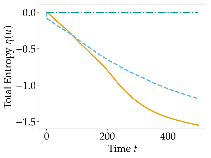
(a) Tolerance $10^{-4}$.

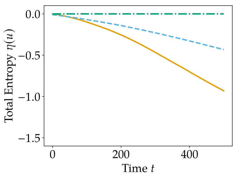
(b) Tolerance $10^{-5}$.

Figure 1: Evolution of the total entropy $\eta(u)$ for the isentropic vortex with an entropy conservative spatial semidiscretization and the BSRK(4,3) time integration scheme with or without local/global relaxation and adaptive time stepping with different tolerances.

4.1.2 Three-dimensional viscous shock propagation

Here, a convergence study for the compressible Navier–Stokes equations is performed using the analytical solution of a propagating viscous shock. We assume a planar shock propagating along the $x_{1}$ coordinate direction with a Prandtl number of $Pr=3/4$. The momentum $\mathcal{V}(x_{1})$ of the analytical solution satisfies the ODE

$$\begin{split}&\alpha\mathcal{V}\frac{\partial\mathcal{V}}{\partial x_{1}}-(\mathcal{V}-1)(\mathcal{V}-\mathcal{V}_{f})=0,\qquad-\infty\leq x_{1}\leq+\infty,\end{split}$$ (4.3)

whose solution can be written implicitly as

$$x_{1}-\frac{1}{2}\alpha\log\left|(\mathcal{V}(x_{1})-1)(\mathcal{V}(x_{1})-\mathcal{V}_{f})\right|+\frac{1+\mathcal{V}_{f}}{1-\mathcal{V}_{f}}\log\left|\frac{\mathcal{V}(x_{1})-1}{\mathcal{V}(x_{1})-\mathcal{V}_{f}}\right|=0,$$ (4.4)

where

$$\mathcal{V}_{f}\equiv\frac{\mathcal{U}_{L}}{\mathcal{U}_{R}},\qquad\alpha\equiv\frac{2\gamma}{\gamma+1}\frac{\,\mu}{Pr\dot{\mathcal{M}}}.$$ (4.5)

Here, $\mathcal{U}_{L/R}$ are the known velocities to the left and right of the shock at $-\infty$ and $+\infty$, respectively, $\dot{\mathcal{M}}$ is the constant mass flow across the shock, $Pr$ is the Prandtl number, and $\mu$ is the dynamic viscosity. The mass and total enthalpy are constant across the shock. Moreover, the momentum and energy equations become redundant.

For our tests, $\mathcal{V}$ is computed from (4.4) to machine precision using bisection. The moving shock solution is obtained by applying a uniform translation to the above solution. Initially, at $t=0$, the shock is located at the center of the domain. We use the parameters $M_{\infty}=2.5$, $Re_{\infty}=10$, and $\gamma=1.4$ and the domain defined by

$$x_{1}\in[-0.5,0.5],\qquad x_{2}\in[-0.5,0.5],\qquad x_{3}\in[-0.5,0.5],\qquad t\in[0,0.5].$$ (4.6)

The boundary conditions are prescribed by penalizing the numerical solution against the analytical solution, which is also used to prescribe the initial condition.

Results of a convergence study for this setup using the locally entropy-stable fully discrete scheme are shown in Table 2. Here, the time step has been reduced under grid refinement to keep the ratio $U_{\infty}\Delta t/\Delta x^{2}$ constant. The resulting errors and convergence rates in the $L^{1}$, $L^{2}$, and $L^{\infty}$ norms are reported in Table 2. As for the compressible Euler equations, we observe that the experimental order of convergence in both the $L^{1}$ and $L^{2}$ norms is the expected order of convergence.

Table 2: Convergence study for the viscous shock problem using entropy dissipative SBP-SAT schemes with different solution polynomial degrees $p$ and local relaxation Runge–Kutta methods (error in the density).

$p$	RK Method	$N$	$L^{1}$ Error	$L^{1}$ Rate	$L^{2}$ Error	$L^{2}$ Rate	$L^{\infty}$ Error	$L^{\infty}$ Rate
2	BSRK(4,3)	5	1.46e-02	—	2.06e-02	—	7.30e-02	—
		10	1.75e-03	3.06	2.50e-03	3.05	9.40e-03	2.96
		15	3.86e-04	3.73	6.41e-04	3.35	3.34e-03	2.56
		20	1.57e-04	3.13	2.58e-04	3.16	1.34e-03	3.16
		25	7.80e-05	3.14	1.29e-04	3.11	7.04e-04	2.89
3	RK(4,4)	5	1.40e-03	—	2.04e-03	—	5.95e-03	—
		10	8.86e-05	3.98	1.43e-04	3.83	6.29e-04	3.24
		15	1.76e-05	3.99	2.89e-05	3.94	1.53e-04	3.49
		20	6.51e-06	3.45	1.05e-05	3.53	5.96e-05	3.27
		25	3.02e-06	3.45	4.90e-06	3.42	2.88e-05	3.26
4	BSRK(8,5)	5	4.70e-04	—	7.19e-04	—	3.37e-03	—
		10	1.94e-05	4.60	2.39e-05	4.91	6.16e-05	5.77
		15	1.30e-06	6.66	2.43e-06	5.64	2.11e-05	2.64
		20	2.54e-07	5.67	4.78e-07	5.65	3.41e-06	6.35
		25	7.60e-08	5.41	1.48e-07	5.24	1.37e-06	4.07
5	VRK(9,6)	5	8.20e-05	—	1.05e-04	—	2.46e-04	—
		10	8.93e-07	6.52	1.54e-06	6.09	1.10e-05	4.48
		15	6.58e-08	6.43	9.82e-08	6.79	7.04e-07	6.79
		20	1.27e-08	5.72	1.87e-08	5.77	1.34e-07	5.77
		25	3.58e-09	5.68	5.14e-09	5.78	3.83e-08	5.62

4.2 Sod’s shock tube

Sod’s shock tube is a classical Riemann problem for the one-dimensional compressible Euler equations that is used to evaluate a numerical method in the presence of a shock, a rarefaction wave, and a contact discontinuity. Of particular interest is the possible smearing of the shock and contact discontinuity, or the generation of oscillations at any discontinuity or very sharp gradient.

The domain is given by $x_{1}\in[0,1]$, $t\in[0,0.2]$, and the initial condition is set to

$$\varrho=\begin{cases}1&x_{1}<0.5,\\ 1/8&x_{1}\geq 0.5,\end{cases}\qquad\mathcal{P}=\begin{cases}1&x_{1}<0.5,\\ 1/10&x_{1}\geq 0.5,\end{cases}\qquad\mathcal{U}_{1}=0.$$ (4.7)

All simulations use a ratio of specific heats equals to $c_{\mathcal{P}}/c_{\mathcal{V}}=7/5$.

The entropy dissipative spatial semidiscretization uses polynomials of degree $p=3$ on a grid with $N=128$ elements. The problem is integrated in time using the classical fourth-order accurate Runge–Kutta method RK(4,4) with a time step ${\Delta t}=$5.0\text{\times}{10}^{-5}$$.

Results of the density with and without relaxation are shown in Figure 2. In general, the density profiles are very similar. In particular, the local relaxation method does not result in a notable smearing of the discontinuities. The local relaxation method reduces the oscillations around the discontinuities up to $1\text{\,}\mathrm{\text{\textperthousand}}$. If the time step is increased by a factor of two, the local relaxation approach reduces the oscillations up to $10\text{\,}\mathrm{\char 37\relax}$. Nevertheless, small overshoots near the non-smooth parts of the numerical approximation are visible. This behavior is expected for a spatial discretization that uses high-order polynomials and no explicit shock capturing mechanism.

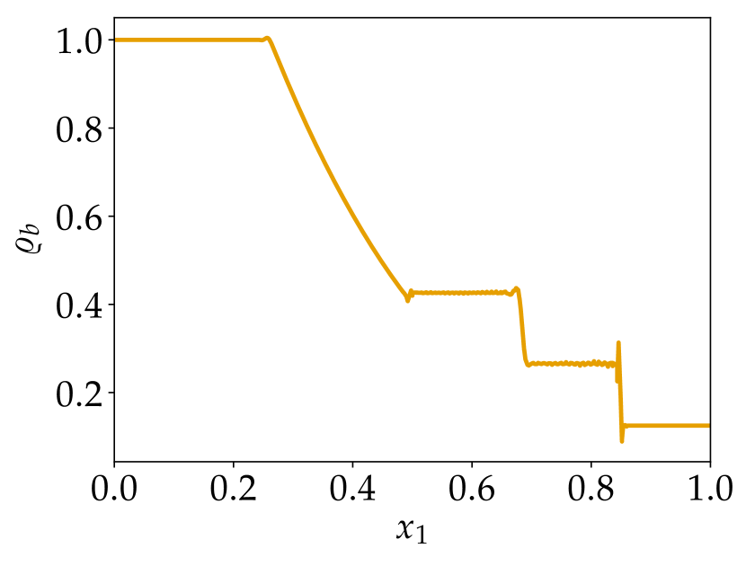
(a) Baseline method.

(b) Local relaxation method.

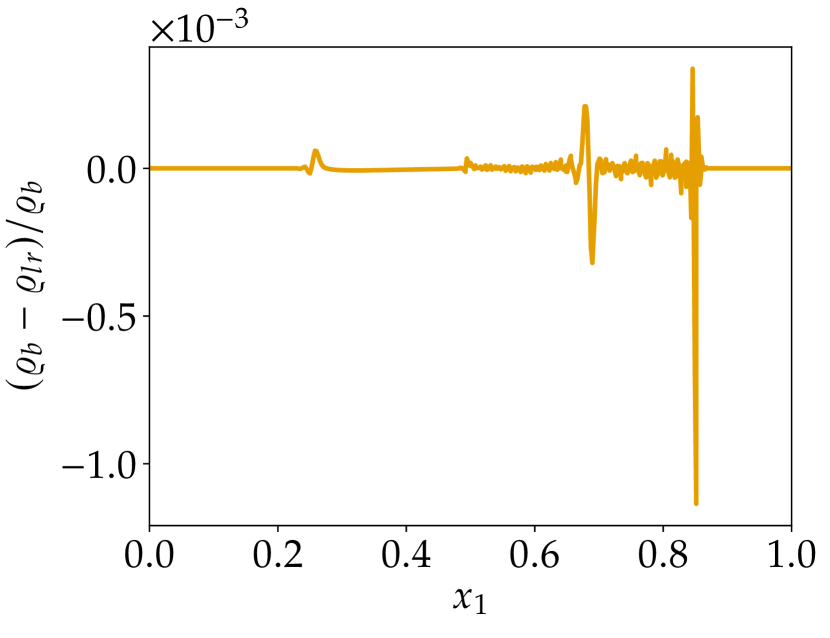
(c) Relative difference.

Figure 2: Density profiles of numerical solutions of Sod’s shock tube problem using polynomials of degrees $p=3$ in $N=128$ elements.

4.3 Sine-shock interaction

Another benchmark problem with both strong discontinuities and smooth structures is given by the sine-shock interaction. This problem is well suited for testing high-order shock-capturing schemes. The governing equations are again the one-dimensional compressible Euler equations, which are solved in the domain given by $x_{1}\in[-5,+5]$, $t\in[0,5]$. The problem is initialized with [72]

$$\left(\varrho,\mathcal{U}_{1},\mathcal{P}\right)=\begin{cases}\left(1.515695,0.523346,1.805\right),&\text{if }-5\leq x<-4.5,\\ \left(1+0.1\sin(20\pi x),0,1\right),&\text{if }-4.5\leq x\leq 5.\end{cases}$$ (4.8)

The entropy dissipative semidiscretization uses polynomials of degree $p=3$ on a grid with $N=256$ elements and the time step with the RK(4,4) is ${\Delta t}=$2.0\text{\times}{10}^{-4}$$. The other parameters are the same as for the Sod’s shock tube problem presented in Section 4.2. The density profiles of the numerical solutions are shown in Figure 3. The results with and without local relaxation are scarcely distinguishable, supporting the conclusions of Section 4.2.

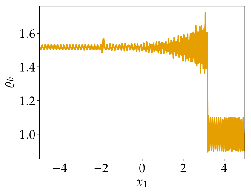
(a) Baseline method.

(b) Local relaxation method.

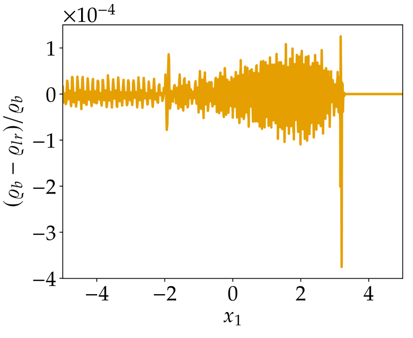
(c) Relative difference.

Figure 3: Density profiles of numerical solutions of the sine-shock interaction problem using polynomials of degrees $p=3$ in $N=256$ elements.

For both Sod’s shock tube and the sine-shock interaction problems, the relaxation parameter $\gamma$ of the local relaxation methods is smaller than unity by approximately $10^{-2}$ for all times, as shown in Figure 4. In contrast, the relaxation parameter for the global relaxation method oscillates following a regular pattern with amplitude $\lesssim 10^{-5}$.

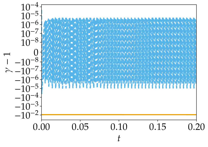
(a) Sod’s shock tube.

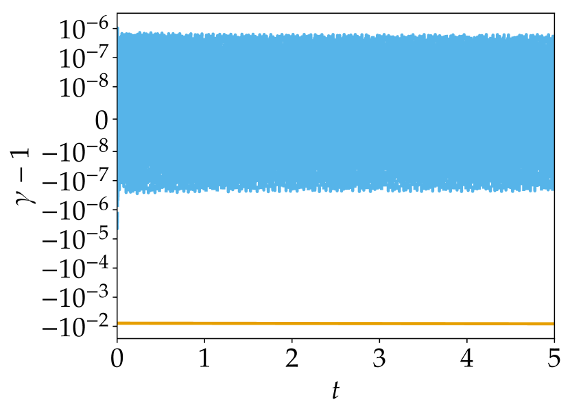
(b) Sine-shock interaction.

Figure 4: Variation of the relaxation parameter $\gamma$ for both global and local relaxation methods for the one-dimensional test problems with discontinuities.

4.4 Local variation of the relaxation parameter

To visualize the variation of the local relaxation parameter $\gamma_{\kappa}$, we use the initial data

$$\left(\varrho,\mathcal{U}_{1},\mathcal{P}\right)=\begin{cases}\left(1+0.5\cos(2\pi x),0.5,1\right),&\text{if }x<0,\\ \left(0.5+0.25\cos(2\pi x),0.5,0.8\right),&\text{if }x\geq 0.\end{cases}$$ (4.9)

The spatial entropy dissipative semidiscretization of the Euler equations uses $200$ elements with polynomials of degree $p=3$ in the domain $[-2,2]$. The classical RK(4,4) method is used with a time step ${\Delta t}=10^{-4}$ to integrate the numerical solution until $t=0.1$.

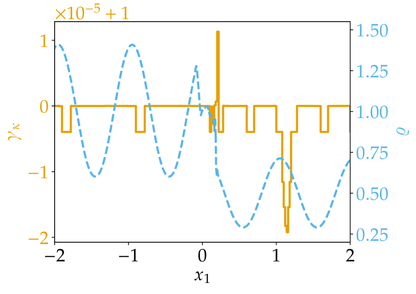
Figure 5: Variation of the local relaxation parameter $\gamma_{\kappa}$ and numerical solution of the density $\varrho$ in space at time $t=0.1$ for the test problem (4.9) with both smooth and discontinuous structures.

The variation of the local relaxation parameter $\gamma_{\kappa}$ at the final time is shown in Figure 5. Overall, $|\gamma_{\kappa}-1|<$2\text{\times}{10}^{-5}$$. The local relaxation parameter is smaller than unity near the smooth local maxima of the numerical solution of the density $\varrho$. Thus, the baseline time integration method introduces some anti-dissipation near the smooth local maxima. Since $\gamma_{\kappa}$ is smaller at the maximum with smaller amplitude on the right-hand side, the baseline time integration method introduces more anti-dissipation on the right-hand side.

Additionally, $\gamma_{\kappa}<1$ near the discontinuity. Interestingly, there is also a very small region near the discontinuity where $\gamma_{\kappa}>1$. Thus, the spatial semidiscretization introduces dissipation in this region and the baseline time integration method introduces some small additional amount of dissipation in front of the right-moving discontinuity.

4.5 Supersonic cylinder

Shock-shock and shock-vortex interactions are very important in the simulation of compressible turbulent flows for many engineering applications. These phenomena have received significant attention in the past and remain an active field of research and development. In this section, we simulate the supersonic flow past a two-dimensional circular cylinder of diameter $\mathrm{D}$.

The supersonic flow past this blunt object is a very complicated test because a detached shock wave is originated ahead of the cylinder, while a rotational flow field of mixed type, i.e., containing supersonic and subsonic regions, appears behind it. Therefore, despite the simplicity of the geometry, capturing the flow at this regime is quite challenging and poses various numerical difficulties that have to be carefully handled and resolved by both the spatial and temporal integration algorithms.

\begin{overpic}[width=346.89731pt,tics=5]{figures/cylinder-mesh.png} \put(7.0,16.0){$6\mathrm{D}$} \put(7.0,2.8){$x_{1}$} \put(-1.0,10.1){$x_{2}$} \put(20.1,-1.0){$10\mathrm{D}$} \put(65.1,-1.0){$30\mathrm{D}$} \end{overpic}

Figure 6: Computational domain, $hp-$non-conforming grid, and solution polynomial degree distribution for the simulation of the supersonic flow past a circular cylinder. Blue: $p=1$ and one level of $h$-refinement, green: $p=2$, orange: $p=3$, magenta: $p=4$ and one level of $h-$refinement.

The similarity parameters based on the quiet flow state upstream of the cylinder (denoted by the subscript $\infty$) are $\mathrm{Re}_{\infty}=10^{4}$ and $\mathrm{Ma}_{\infty}=3.5$. The computational domain is $x_{1}/\mathrm{D}\in[-3,3],\,x_{2}/\mathrm{D}\in[-20,20]$ and $t\,\mathcal{U}_{\infty}/\mathrm{D}\in[0,40]$. Figure 6 shows an overview of the computational domain, grid, and solution polynomial degree, $p$, distribution. The region of the computational domain upstream of the bow shock is discretized with $p=2$; the region that surrounds the bow shock is discretized with $p=1$ and one level of $h$-refinement; the cylinder’s boundary layer and wake regions are discretized with $p=4$ and one level of $h$-refinement, and in the rest of the domain, $p=2$ is used. The total number of hexahedral elements and degrees of freedom (DOFs) are $5{,}0678$ and $33{,}958$, respectively.

The entropy stable adiabatic no-slip wall boundary conditions presented in [46, 20] are applied to the solid surfaces. Inviscid wall boundary conditions are imposed on the top and bottom horizontal boundaries. Periodic boundary conditions are used for the boundaries perpendicular to the axis of the cylinder. Far-field boundary conditions are used for the inlet and outlet boundaries. The classical RK(4,4) method with relaxation is used for the time integration. e emphasize that the same temporal discretization without local relaxation requires a time step which is approximately nine times smaller than the average time step used with the relaxation approach.

A quantitative analysis of the computational results can be performed using the oblique shock wave theory. The most useful relation of the oblique shock wave theory is the one providing the deflection angle $\theta$ explicitly as a function of the shock angle, $\beta$, and local Mach number, $\mathrm{Ma}$:

$$\tan\left(\theta\right)=2\cot\left(\beta\right)\left[\frac{\mathrm{Ma}^{2}\sin^{2}\left(\beta\right)-1}{\mathrm{Ma}^{2}\left(\gamma+\cos\left(2\beta\right)\right)+2}\right].$$ (4.10)

The shock wave angle, $\beta$, with respect to the incoming flow may be evaluated at each location, while the other two directions or associated flow deflection angle, $\theta$, can be determined (along the shock wave abscissa, $s$) from the local simulated flow properties upstream and downstream of the detached shock wave.

Figure 7 shows the temperature contour plot of our numerical simulation. We can clearly see the strong bow shock located in front of the cylinder and the complicated vortical flow structures and reflected shocks behind the object.

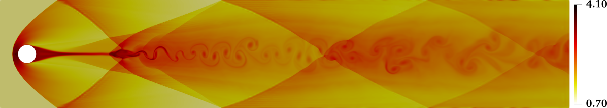
Figure 7: Visualization of the instantaneous temperature field, $\mathcal{T}$, for the supersonic flow past a circular cylinder.

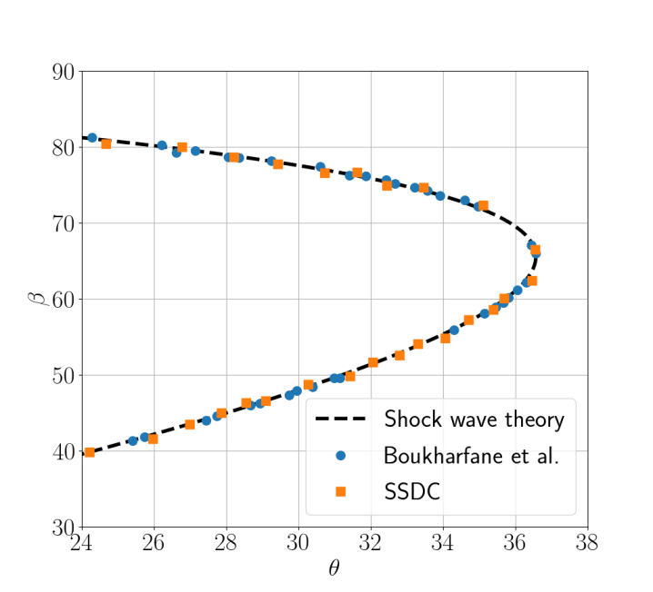
Figure 8: $\theta$-$\beta$-$\mathrm{Ma}$ plot for the supersonic flow past a circular cylinder.

Figure 8 compares the pair $\theta(s)$-$\beta(s)$ computed by post-processing the solution obtained with the SSDC solver, showing i) the results obtained with the oblique shock–wave theory and ii) the reference results reported in [9], which are computed with a seventh-order accurate weighted essentially non-oscillatory (WENO7) scheme with characteristic flux reconstruction combined with an eighth-order centered difference scheme on a grid with more than $4\times 10^{6}$ nodes. The SSDC results are in very good agreement with the theoretical curve and the numerical data set.

4.6 Homogeneous isotropic turbulence

We used the homogeneous isotropic turbulence test case to assess the resolution for broadband turbulent flows of the present solver, which is quantitatively measured by the predicted turbulent kinetic energy spectrum. We consider the decaying of compressible isotropic turbulence with an initial turbulent Mach number of $\mathrm{Ma}_{t}=0.3$ (compressible isotropic turbulence in nonlinear subsonic regime) and Taylor Reynolds number of $\mathrm{Re}_{\lambda}=72$. These flow parameters are, respectively, defined as

$$\mathrm{Ma}_{t}=\frac{\mathcal{U}^{\prime}}{\langle c\rangle}=\mathrm{M}\frac{\mathcal{U}^{\prime}}{\langle\sqrt{T}\rangle},$$ (4.11)

$$\mathrm{Re}_{\lambda}=\frac{\mathcal{U}^{\prime}\lambda\langle\varrho\rangle}{\langle\mu\rangle}=\mathrm{Re}\frac{\mathcal{U}^{\prime}\lambda\langle\varrho\rangle}{\sqrt{3}\langle\mu\rangle},$$ (4.12)

where the root-mean square (RMS) of the velocity magnitude fluctuations is computed as $\mathcal{U}^{\prime}=\langle\mathcal{U}_{i}\mathcal{U}_{i}/3\rangle^{1/2}$, and the normalized Taylor micro–scale $\lambda$ is defined by

$$\lambda=\sqrt{\frac{\mathcal{U}^{{}^{\prime}2}}{\left\langle\left(\frac{\partial\mathcal{U}_{1}}{\partial x_{1}}\right)^{2}+\left(\frac{\partial\mathcal{U}_{2}}{\partial x_{2}}\right)^{2}+\left(\frac{\partial\mathcal{U}_{3}}{\partial x_{3}}\right)^{2}\right\rangle}},$$ (4.13)

where $\langle\cdot\rangle$ denotes a volume average over the computational domain, $\Omega$. The simulation domain has extent $[0,2\pi]\times[0,2\pi]\times[0,2\pi]$. The parameter values used here have been investigated by [61] using DNS with a tenth-order accurate Padè scheme.

Periodic boundary conditions are adopted in all three coordinate directions. The initial hydrodynamic field is divergence-free and has an energy spectrum given by

$$E(k)=A_{0}k^{4}\exp\left(-2k^{2}/k_{0}^{2}\right),$$ (4.14)

where $k$, $k_{0}$, and $A$ are the wave number, the spectrum’s peak wave number, and the constant chosen to get the specified initial turbulent kinetic energy, respectively. Here, we set $k_{0}=8$ and $A_{0}=$0.000\,13$$. The thermodynamic field is specified in the same manner as the cases $D1$ and $D5$ presented in [61, 8]. For the decaying of compressible turbulence, as time evolves, both $\mathrm{M}_{t}$ and $\mathrm{Re}_{\lambda}$ decrease. Therefore, the flow fields are smooth without strong shocklets. The classical RK(4,4) method with relaxation is used for the time integration.

Figure 9 shows the decaying history of the resolved turbulent kinetic energy $\mathcal{E}_{K}=1/2\langle\varrho\mathcal{U}_{i}\mathcal{U}_{i}\rangle$ and the Reynolds number based on Taylor micro–scale versus $t/\tau$. Herein, $\tau=\mathcal{L}_{1}/\mathcal{U}^{\prime}$ is the initial large-eddy-turnover time with $\mathcal{L}_{1}$ being the integral length scale defined as

$$\mathcal{L}_{1}=\frac{3\pi}{4}\frac{\int_{0}^{\infty}\frac{E(k)}{k}\mathrm{d}k}{\int_{0}^{\infty}E(k)\mathrm{d}k}.$$ (4.15)

Except for slight under-predictions for $t/\tau<1$ due to the initialization, we observe a very good agreement between the SSDC solutions computed with $16^{3}$ hexahedral elements and $p=5$ and the reference solution of [61]. The latter is computed using a grid with $128^{3}$ points.

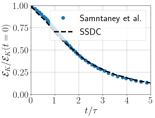
(a) Turbulent kinetic energy.

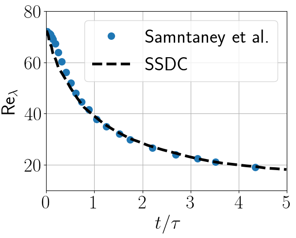
(b) Reynolds number based on Taylor micro-scale.

Figure 9: Compressible isotropic turbulence at Ma${}_{t}=0.3$ and Re${}_{\lambda}=72$.

5 Summary and conclusions

We have proposed, analyzed, and developed the general framework of local relaxation time integration schemes in the setting of ordinary differential equations. This extension of the recent relaxation approach to numerical time integration schemes enables to guarantee entropy inequalities for finitely many convex local entropies while preserving all linear invariants. While we have applied the theory to local inequalities of a single entropy, it extends directly without further modifications to finitely many local or global inequalities of different convex entropies.

This approach has been applied to entropy conservative and dissipative semidiscretizations of the compressible Euler and Navier–Stokes equations. The resulting conservative fully discrete schemes guarantee local entropy inequalities without adding superfluous artificial dissipation. This is possible to accomplish in the relaxation framework because the amount of dissipation in time is adapted to the spatial dissipation a posteriori instead of a priori. Hence, local relaxation methods do not degrade the solution accuracy. Instead, they can also remove superfluous dissipation if necessary.

In general, baseline RK schemes can guarantee neither entropy conservation nor entropy dissipation. Global relaxation methods can enforce both conservation and dissipation of a single global convex entropy. By modifying the relaxation parameter slightly, global relaxation methods can even introduce some dissipation in time if entropy conservative spatial semidiscretizations are employed. In contrast, local relaxation methods impose local entropy inequalities. These can be summed up to get a global entropy inequality, but a global entropy equality is impossible in general. On the other hand, local entropy inequalities are the more important tools to obtain bounds, estimates, and further results.

This novel technique, combined with the entropy conservative/dissipative spatial semidiscretizations employed in this article, yields the first discretization for compressible computational fluid dynamics that is

• primary conservative,

• locally entropy dissipative in the fully discrete sense with ${\Delta t}=\mathcal{O}(\Delta x)$,

• explicit, except for the solution of a scalar equation per time step and local entropy,

• and arbitrarily high-order accurate in space and time.

Since the scalar equations that must be solved for each local relaxation parameter are fully localized to the elements, they can be parallelized efficiently.

Here, we have used relaxation methods to guarantee fully discrete local entropy inequalities for discontinuous collocation methods (mass lumped discontinuous Galerkin finite element methods). Applications of these methods and other means to guarantee local entropy inequalities for fully discrete numerical methods will be further studied in the future.

References

- [1] Rémi Abgrall, Philipp Öffner and Hendrik Ranocha “Reinterpretation and Extension of Entropy Correction Terms for Residual Distribution and Discontinuous Galerkin Schemes”, 2019 arXiv:1908.04556 [math.NA]
- [2] Shrirang Abhyankar et al. “PETSc/TS: A Modern Scalable ODE/DAE Solver Library”, 2018 arXiv:1806.01437 [math.NA]
- [3] GE Alefeld, Florian A Potra and Yixun Shi “Algorithm 748: Enclosing Zeros of Continuous Functions” In ACM Transactions on Mathematical Software (TOMS) 21.3 ACM New York, NY, USA, 1995, pp. 327–344 DOI: 10.1145/210089.210111
- [4] Satish Balay et al. “PETSc Users Manual”, 2018
- [5] P Bogacki and Lawrence F Shampine “An efficient Runge–Kutta (4,5) pair” In Computers & Mathematics with Applications 32.6 Elsevier, 1996, pp. 15–28 DOI: 10.1016/0898-1221(96)00141-1
- [6] Przemyslaw Bogacki and Lawrence F Shampine “A 3(2) pair of Runge–Kutta formulas” In Applied Mathematics Letters 2.4 Elsevier, 1989, pp. 321–325 DOI: 10.1016/0893-9659(89)90079-7
- [7] Pieter D Boom and David W Zingg “High-order implicit time-marching methods based on generalized summation-by-parts operators” In SIAM Journal on Scientific Computing 37.6 SIAM, 2015, pp. A2682–A2709 DOI: 10.1137/15M1014917
- [8] R. Boukharfane, Z. Bouali and A. Mura “Evolution of scalar and velocity dynamics in planar shock-turbulence interaction” In Shock Waves 28.6, 2018, pp. 1117–1141 DOI: 10.1007/s00193-017-0798-5
- [9] R. Boukharfane, F. H. E. Ribeiro, Z. Bouali and A. Mura “A combined ghost-point-forcing/direct-forcing immersed boundary method (IBM) for compressible flow simulations” In Computers & Fluids 162 Elsevier, 2018, pp. 91–112 DOI: 10.1016/j.compfluid.2017.11.018
- [10] Kevin Burrage and John Charles Butcher “Non-linear stability of a general class of differential equation methods” In BIT Numerical Mathematics 20.2 Springer, 1980, pp. 185–203 DOI: 10.1007/BF01933191
- [11] Kevin Burrage and John Charles Butcher “Stability criteria for implicit Runge–Kutta methods” In SIAM Journal on Numerical Analysis 16.1 SIAM, 1979, pp. 46–57 DOI: 10.1137/0716004
- [12] Carsten Burstedde, Lucas C. Wilcox and Omar Ghattas “p4est: Scalable Algorithms for Parallel Adaptive Mesh Refinement on Forests of Octrees” In SIAM Journal on Scientific Computing 33.3, 2011, pp. 1103–1133 DOI: 10.1137/100791634
- [13] John Charles Butcher “Numerical Methods for Ordinary Differential Equations” Chichester: John Wiley & Sons Ltd, 2016 DOI: 10.1002/9781119121534
- [14] Mark H Carpenter, Travis C Fisher, Eric J Nielsen and Steven H Frankel “Entropy Stable Spectral Collocation Schemes for the Navier–Stokes Equations: Discontinuous Interfaces” In SIAM Journal on Scientific Computing 36.5 Society for IndustrialApplied Mathematics, 2014, pp. B835–B867 DOI: 10.1137/130932193
- [15] Mark H Carpenter, Matteo Parsani, Travis C Fisher and Eric J Nielsen “Entropy Stable Staggered Grid Spectral Collocation for the Burgers’ and Compressible Navier–Stokes Equations” In NASA TM-2015-218990, 2015
- [16] Mark H Carpenter, Matteo Parsani, Travis C Fisher and Eric J Nielsen “Towards an entropy stable spectral element framework for computational fluid dynamics” In 54th AIAA Aerospace Sciences Meeting, 2016 American Institute of AeronauticsAstronautics DOI: 10.2514/6.2016-1058
- [17] Jesse Chan “On discretely entropy conservative and entropy stable discontinuous Galerkin methods” In Journal of Computational Physics 362 Elsevier, 2018, pp. 346–374 DOI: 10.1016/j.jcp.2018.02.033
- [18] Jared Crean et al. “Entropy-stable summation-by-parts discretization of the Euler equations on general curved elements” In Journal of Computational Physics 356 Elsevier, 2018, pp. 410–438 DOI: 10.1016/j.jcp.2017.12.015
- [19] Constantine M Dafermos “Hyperbolic Conservation Laws in Continuum Physics” Berlin Heidelberg: Springer-Verlag, 2010 DOI: 10.1007/978-3-642-04048-1
- [20] L. Dalcin et al. “Conservative and entropy stable solid wall boundary conditions for the compressible Navier–Stokes equations: Adiabatic wall and heat entropy transfer” In Journal of Computational Physics 397 Elsevier, 2019, pp. 108775 DOI: 10.1016/j.jcp.2019.06.051
- [21] Kees Dekker and Jan G Verwer “Stability of Runge–Kutta methods for stiff nonlinear differential equations” 2, CWI Monographs Amsterdam: North-Holland, 1984
- [22] D. C. Del Rey Fernández et al. “Entropy stable nonconforming discretizations with the summation-by-parts property for the compressible Euler equations”, 2020 arXiv:1909.12536 [math.NA]
- [23] D. C. Del Rey Fernández et al. “Entropy stable nonconforming discretizations with the summation-by-parts property for the compressible Navier–Stokes equations” In In press in Computer & Fluids, 2020
- [24] David C. Del Rey Fernández et al. “Entropy stable non-conforming discretization with the summation-by-parts property for the compressible Euler and Navier–Stokes equations” In SN Partial Differential Equations and Applications 1.2, 2020 DOI: 10.1007/s42985-020-00009-z
- [25] D. C. D. R. Fernández et al. “Entropy stable non-conforming discretizations with the summation-by-parts property for curvilinear coordinates” In NASA TM-2020-220574, 2020
- [26] T. C. Fisher “High-order stable multi-domain finite difference method for compressible flows”, 2012
- [27] Travis C Fisher and Mark H Carpenter “High-order entropy stable finite difference schemes for nonlinear conservation laws: Finite domains” In Journal of Computational Physics 252 Elsevier, 2013, pp. 518–557 DOI: 10.1016/j.jcp.2013.06.014
- [28] Lucas Friedrich et al. “Entropy Stable Space–Time Discontinuous Galerkin Schemes with Summation-by-Parts Property for Hyperbolic Conservation Laws” In Journal of Scientific Computing 80.1 Springer, 2019, pp. 175–222 DOI: 10.1007/s10915-019-00933-2
- [29] Lucas Friedrich et al. “An entropy stable h/p non-conforming discontinuous Galerkin method with the summation-by-parts property” In Journal of Scientific Computing 77.2 Springer, 2018, pp. 689–725 DOI: 10.1007/s10915-018-0733-7
- [30] Jan Glaubitz, Philipp Öffner, Hendrik Ranocha and Thomas Sonar “Artificial Viscosity for Correction Procedure via Reconstruction Using Summation-by-Parts Operators” In Theory, Numerics and Applications of Hyperbolic Problems II 237, Springer Proceedings in Mathematics & Statistics Cham: Springer International Publishing, 2018, pp. 363–375 DOI: 10.1007/978-3-319-91548-7_28
- [31] Ernst Hairer, Christian Lubich and Gerhard Wanner “Geometric Numerical Integration: Structure-Preserving Algorithms for Ordinary Differential Equations” 31, Springer Series in Computational Mathematics Berlin Heidelberg: Springer-Verlag, 2006 DOI: 10.1007/3-540-30666-8
- [32] Amiram Harten “On the symmetric form of systems of conservation laws with entropy” In Journal of Computational Physics 49.1 Elsevier, 1983, pp. 151–164 DOI: 10.1016/0021-9991(83)90118-3
- [33] J. E. Hicken “Entropy-Stable, High-Order Summation-by-Parts Discretizations Without Interface Penalties” In Journal of Scientific Computing 82, 2020 DOI: 10.1007/s10915-020-01154-8
- [34] Inmaculada Higueras “Monotonicity for Runge–Kutta Methods: Inner Product Norms” In Journal of Scientific Computing 24.1 Springer, 2005, pp. 97–117 DOI: 10.1007/s10915-004-4789-1
- [35] Ansgar Jüngel and Stefan Schuchnigg “Entropy-dissipating semi-discrete Runge–Kutta schemes for nonlinear diffusion equations” In Communications in Mathematical Sciences 15.1 International Press of Boston, 2017, pp. 27–53 DOI: 10.4310/CMS.2017.v15.n1.a2
- [36] David I Ketcheson “Relaxation Runge–Kutta Methods: Conservation and Stability for Inner-Product Norms” In SIAM Journal on Numerical Analysis 57.6 Society for IndustrialApplied Mathematics, 2019, pp. 2850–2870 DOI: 10.1137/19M1263662
- [37] Matthew G. Knepley and Dmitry A. Karpeev “Mesh Algorithms for PDE with Sieve I: Mesh Distribution” In Scientific Programming 17.3, 2009, pp. 215–230 DOI: 10.3233/SPR-2009-0249
- [38] Wilhelm Kutta “Beitrag zur näherungsweisen Integration totaler Differentialgleichungen” In Zeitschrift für Mathematik und Physik 46, 1901, pp. 435–453
- [39] Philippe G LeFloch, Jean-Marc Mercier and Christian Rohde “Fully Discrete, Entropy Conservative Schemes of Arbitrary Order” In SIAM Journal on Numerical Analysis 40.5 Society for IndustrialApplied Mathematics, 2002, pp. 1968–1992 DOI: 10.1137/S003614290240069X
- [40] Carlos Lozano “Entropy Production by Explicit Runge–Kutta Schemes” In Journal of Scientific Computing 76.1 Springer, 2018, pp. 521–565 DOI: 10.1007/s10915-017-0627-0
- [41] Carlos Lozano “Entropy Production by Implicit Runge–Kutta Schemes” In Journal of Scientific Computing Springer, 2019 DOI: 10.1007/s10915-019-00914-5
- [42] Jan Nordström and Cristina La Cognata “Energy stable boundary conditions for the nonlinear incompressible Navier–Stokes equations” In Mathematics of Computation 88.316 American Mathematical Society, 2019, pp. 665–690 DOI: 10.1090/mcom/3375
- [43] Philipp Öffner, Jan Glaubitz and Hendrik Ranocha “Analysis of Artificial Dissipation of Explicit and Implicit Time-Integration Methods” Accepted in International Journal of Numerical Analysis and Modeling, 2019 arXiv:1609.02393 [math.NA]
- [44] M. Parsani et al. “Unveiling the potential of high-order accurate entropy stable discontinuous collocated Galerkin methods for the next generation of compressible CFD frameworks: SSDC algorithms and flow solver” In Submitted, 2020
- [45] Matteo Parsani, Mark H Carpenter and Eric J Nielsen “Entropy stable discontinuous interfaces coupling for the three-dimensional compressible Navier–Stokes equations” In Journal of Computational Physics 290 Elsevier, 2015, pp. 132–138 DOI: 10.1016/j.jcp.2015.02.042
- [46] Matteo Parsani, Mark H Carpenter and Eric J Nielsen “Entropy stable wall boundary conditions for the three-dimensional compressible Navier–Stokes equations” In Journal of Computational Physics 292, 2015, pp. 88–113 DOI: 10.1016/j.jcp.2015.03.026
- [47] W. Pazner and P-O. Persson “Analysis and Entropy Stability of the Line-Based Discontinuous Galerkin Method” In Journal of Scientific Computing 80.1, 2019, pp. 376–402 DOI: 10.1007/s10915-019-00942-1
- [48] Hendrik Ranocha “Comparison of Some Entropy Conservative Numerical Fluxes for the Euler Equations” In Journal of Scientific Computing 76.1 Springer, 2018, pp. 216–242 DOI: 10.1007/s10915-017-0618-1
- [49] Hendrik Ranocha “Generalised Summation-by-Parts Operators and Entropy Stability of Numerical Methods for Hyperbolic Balance Laws”, 2018
- [50] Hendrik Ranocha “On Strong Stability of Explicit Runge-Kutta Methods for Nonlinear Semibounded Operators” In IMA Journal of Numerical Analysis Oxford University Press, 2020 DOI: 10.1093/imanum/drz070
- [51] Hendrik Ranocha “Some Notes on Summation by Parts Time Integration Methods” In Results in Applied Mathematics 1 Elsevier, 2019, pp. 100004 DOI: 10.1016/j.rinam.2019.100004
- [52] Hendrik Ranocha, Jan Glaubitz, Philipp Öffner and Thomas Sonar “Stability of artificial dissipation and modal filtering for flux reconstruction schemes using summation-by-parts operators” See also arXiv: 1606.00995 [math.NA] and arXiv: 1606.01056 [math.NA] In Applied Numerical Mathematics 128 Elsevier, 2018, pp. 1–23 DOI: 10.1016/j.apnum.2018.01.019
- [53] Hendrik Ranocha and David I Ketcheson “Energy Stability of Explicit Runge–Kutta Methods for Non-autonomous or Nonlinear Problems”, 2019 arXiv:1909.13215 [math.NA]
- [54] Hendrik Ranocha and David I Ketcheson “Relaxation Runge-Kutta Methods for Hamiltonian Problems” Accepted in Journal of Scientific Computing, 2020 arXiv:2001.04826 [math.NA]
- [55] Hendrik Ranocha, Lajos Lóczi and David I Ketcheson “General Relaxation Methods for Initial-Value Problems with Application to Multistep Schemes”, 2020 arXiv:2003.03012 [math.NA]
- [56] Hendrik Ranocha and Jan Nordström “A Class of Stable Summation by Parts Time Integration Schemes”, 2020 arXiv:2003.03889 [math.NA]
- [57] Hendrik Ranocha and Philipp Öffner “ Stability of Explicit Runge–Kutta Schemes” In Journal of Scientific Computing 75.2, 2018, pp. 1040–1056 DOI: 10.1007/s10915-017-0595-4
- [58] Hendrik Ranocha et al. “Relaxation Runge–Kutta Methods: Fully-Discrete Explicit Entropy-Stable Schemes for the Compressible Euler and Navier–Stokes Equations” In SIAM Journal on Scientific Computing 42.2 Society for IndustrialApplied Mathematics, 2020, pp. A612–A638 DOI: 10.1137/19M1263480
- [59] I. E. Reyna Nolasco et al. “Optimized geometrical metrics satisfying free-stream preservation” In Computer & Fluids 207, 2020 DOI: 10.1016/j.compfluid.2020.104555
- [60] D. Rojas et al. “On the robustness and performance of entropy stable discontinuous collocation methods for the compressible Navier–Stokes equations” Submitted, 2020 arXiv:1911.10966 [math.NA]
- [61] R. Samtaney, D. I. Pullin and B. Kosović “Direct numerical simulation of decaying compressible turbulence and shocklet statistics” In Physics of Fluids 13.5 AIP, 2001, pp. 1415–1430 DOI: 10.1063/1.1355682
- [62] Jesus Maria Sanz-Serna “An explicit finite-difference scheme with exact conservation properties” In Journal of Computational Physics 47.2 Elsevier, 1982, pp. 199–210 DOI: 10.1016/0021-9991(82)90074-2
- [63] Jesus Maria Sanz-Serna and VS Manoranjan “A method for the integration in time of certain partial differential equations” In Journal of Computational Physics 52.2 Elsevier, 1983, pp. 273–289 DOI: 10.1016/0021-9991(83)90031-1
- [64] Cengke Shi and Chi-Wang Shu “On local conservation of numerical methods for conservation laws” In Computers & Fluids 169 Elsevier, 2018, pp. 3–9 DOI: 10.1016/j.compfluid.2017.06.018
- [65] Björn Sjögreen and HC Yee “High order entropy conservative central schemes for wide ranges of compressible gas dynamics and MHD flows” In Journal of Computational Physics 364 Elsevier, 2018, pp. 153–185 DOI: 10.1016/j.jcp.2018.02.003
- [66] Zheng Sun and Chi-Wang Shu “Enforcing strong stability of explicit Runge–Kutta methods with superviscosity”, 2019 arXiv:1912.11596 [math.NA]
- [67] Zheng Sun and Chi-Wang Shu “Stability of the fourth order Runge–Kutta method for time-dependent partial differential equations” In Annals of Mathematical Sciences and Applications 2.2, 2017, pp. 255–284 DOI: 10.4310/AMSA.2017.v2.n2.a3
- [68] Zheng Sun and Chi-Wang Shu “Strong Stability of Explicit Runge–Kutta Time Discretizations” In SIAM Journal on Numerical Analysis 57.3 SIAM, 2019, pp. 1158–1182 DOI: 10.1137/18M122892X
- [69] Magnus Svärd and Hatice Özcan “Entropy-stable schemes for the Euler equations with far-field and wall boundary conditions” In Journal of Scientific Computing 58.1 Springer, 2014, pp. 61–89 DOI: 10.1007/s10915-013-9727-7
- [70] Eitan Tadmor “Entropy stability theory for difference approximations of nonlinear conservation laws and related time-dependent problems” In Acta Numerica 12 Cambridge University Press, 2003, pp. 451–512 DOI: 10.1017/S0962492902000156
- [71] Eitan Tadmor “From Semidiscrete to Fully Discrete: Stability of Runge–Kutta Schemes by the Energy Method II” In Collected Lectures on the Preservation of Stability under Discretization 109, Proceedings in Applied Mathematics Philadelphia: Society for IndustrialApplied Mathematics, 2002, pp. 25–49
- [72] Vladimir A Titarev and Eleuterio F Toro “Finite-volume WENO schemes for three-dimensional conservation laws” In Journal of Computational Physics 201.1 Elsevier, 2004, pp. 238–260 DOI: 10.1016/j.jcp.2004.05.015
- [73] James Hamilton Verner “Explicit Runge–Kutta methods with estimates of the local truncation error” In SIAM Journal on Numerical Analysis 15.4 SIAM, 1978, pp. 772–790 DOI: 10.1137/0715051
- [74] Hamed Zakerzadeh and Ulrik Skre Fjordholm “High-order accurate, fully discrete entropy stable schemes for scalar conservation laws” In IMA Journal of Numerical Analysis 36.2 Oxford University Press, 2016, pp. 633–654 DOI: 10.1093/imanum/drv020