Gamma Related Ornstein-Uhlenbeck Processes and their Simulation

Abstract

We investigate the distributional properties of two generalized Ornstein-Uhlenbeck (OU) processes whose stationary distributions are the gamma law and the bilateral gamma law, respectively. The said distributions turn out to be related to the self-decomposable gamma and bilateral gamma laws, and their densities and characteristic functions are here given in closed-form. Algorithms for the exact generation of such processes are accordingly derived with the advantage of being significantly faster than those available in the literature and therefore suitable for real-time simulations.

1 Introduction and Motivation

In the present paper we study the distributional properties of the Gamma-Ornstein-Uhlenbeck process ($\Gamma$-OU) and the Bilateral Gamma-OU process ($\mathrm{bi}\Gamma$-OU). Our contribution consists in the derivation of the closed-form of both the density and the characteristic function of such processes. In its turn, this main result enables us to obtain fast algorithms for their exact simulation, along with an unbiased transition density that can be used for parameter estimation.

To this end, following Barndorff-Nielsen and Shephard [2], we consider a Lévy process $Z(t)$ and the generalized OU process defined by the SDE

$$dX(t)=-kX(t)dt+dZ(t)\quad\qquad X(0)=X_{0}\quad\bm{P}\hbox{-\emph{a.s.}}\qquad k>0.$$ (1)

Here $Z(t)$ is called the Backward Driving Lévy Process (BDLP), and we will adopt the following notation: if $\mathfrak{D}$ is the stationary law of $X(t)$ we will say that $X(t)$ is a $\mathfrak{D}$-OU process; if on the other hand, $Z(1)$ (namely the BDLP at time $t=1$) is distributed according to the id (infinitely divisible) law $\widetilde{\mathfrak{D}}$, then we will say that $X(t)$ is an OU-$\widetilde{\mathfrak{D}}$ process. Now a well known result (see for instance Cont and Tankov [9], Sato [31]) is that, a given one-dimensional distribution $\mathfrak{D}$ always is the stationary law of a suitable OU-$\widetilde{\mathfrak{D}}$ process if and only if $\mathfrak{D}$ is self-decomposable.

We recall that a law with probability density (pdf) $f(x)$ and characteristic function (chf) $\varphi(u)$ is said to be self-decomposable (sd) (see Sato[31] or Cufaro Petroni [10]) when for every $0<a<1$ we can find another law with pdf $g_{a}(x)$ and chf $\chi_{a}(u)$ such that

$$\varphi(u)=\varphi(au)\chi_{a}(u)$$ (2)

We will accordingly say that a random variable (rv) $X$ with pdf $f(x)$ and chf $\varphi(u)$ is sd when its law is sd: looking at the definition, this means that for every $0<a<1$ we can always find two independent rv’s, $Y$ (with the same law of $X$) and $Z_{a}$ ( here called $a$-remainder), with pdf $g_{a}(x)$ and chf $\chi_{a}(u)$) such that

$$X\stackrel{{\scriptstyle d}}{{=}}aY+Z_{a}\qquad\quad\bm{P}\hbox{-\emph{a.s.}}$$ (3)

It is well known that the $\Gamma$-OU process $X(t)$ solution of (1) implies that $Z(t)$ is a compound Poisson with exponential jumps (see for instance Schoutens [32]) and we will prove that for the $\mathrm{bi}\Gamma$-OU process $Z(t)$ is instead a compound Poisson with double exponential distribution as defined in Kou [20].

We will show that the law of the $\Gamma$-OU process and the $\mathrm{bi}\Gamma$-OU process at time $t$ coincide with that of the $a$-remainder $Z_{a}$ of a sd gamma and a bilateral gamma distribution, respectively. Although a similar result has yet to be proved for other generalized OU processes, in our particular case it allows to find the pdf and the chf of $X(t)$ in closed-form because the $a$-remainder’s of a gamma and a bilateral gamma distribution turn out to be manageable mixtures of other elementary distributions. As a consequence, we can design efficient and fast algorithms to exactly simulate $\Gamma$-OU and $\mathrm{bi}\Gamma$-OU processes, outperforming in so doing every other existing alternative (see Cont and Tankov [9] and Qu et al. [29]). The numerical experiments we have conducted clearly show that the computational times of our approach are very small therefore, our solution is suitable for real time simulations.

As observed in Barndorff-Nielsen and Shephard [2], the $\Gamma$-OU process is a very tractable model that could adopted in many potential applications. For instance, in the energy and in the commodity field, many authors (using sometimes different naming conventions) coupled a $\Gamma$-OU process or a combination of $\Gamma$-OU processes to a standard Gaussian-OU to model day-ahead spot prices. Among others, Kluge [19] and Kjaer [18] apply such a combination to price swing options and gas storages while Benth and Pircalabu [3] apply a $\Gamma$-OU process to evaluate wind derivatives. In alternative, Meyer-Brandis and Tankov [25] adopted a two regime-switching model consisting in a Gaussian-OU process and a $\Gamma$-OU process to model power prices. The use of $\Gamma$-OU or $\mathrm{bi}\Gamma$-OU in energy market is justified by the fact that gas and power prices exhibit strong mean-reversion and spikes. Beyond commodity markets, other applications of the $\Gamma$-OU and $\mathrm{bi}\Gamma$-OU processes are available in the literature: among others Barndorff-Nielsen and Shephard [2] used a $\Gamma$-OU process to model stochastic volatility while Schoutens and Cariboni [33] and Bianchi and Fabozzi [4] adopted the $\Gamma$-OU process as a stochastic intensity process for modelling credit default risk and pricing credit default swaps.

The paper is structured as follows: in Section 2 we study the distributional properties of a $\Gamma$-OU process showing that it can be represented as a mixture of Polya or binomial mixtures and therefore, it can be seen as a compound sum of independent exponential rv’s or as an Erlang rv with a random index. These findings are instrumental to design the simulation algorithms illustrated in Subsection 2.3. Section 3 analyzes the distributional properties of a $\mathrm{bi}\Gamma$-OU process and focuses on the case with symmetric parameters. These results are then used in Subsection 3.2 to concieve the relative simulation algorithms. Section 4 illustrates the numerical experiments that we have conducted to compare the convergence and computational performance of our solutions to the approaches in Cont and Tankov [9] and in Qu at al. [29]. Finally Section 5 concludes the paper with an overview of future inquiries and possible further applications.

2 Distributional properties of the $\Gamma$-OU process

According to an aforementioned result, a $\Gamma$-OU($k,\lambda,\beta$) process $X(t)$ is the solution of (1) where the BDLP is a compound Poisson process $Z(t)$ with intensity $\lambda$ of the number process $N(t)$, and identically distributed exponential jumps $J_{n}\sim\mathfrak{E}_{1}(\beta)$

$$Z(t)=\sum_{n=0}^{N(t)}J_{n}\qquad\quad J_{0}=0\quad\bm{P}\hbox{-\emph{a.s.}}$$

It turns out that $Z(t)$ is a subordinator, and that the solution of (1) reads now as

$$X(t)=x_{0}e^{-kt}+\sum_{n=0}^{N(t)}e^{-k(t-\tau_{n})}J_{n}$$ (4)

where $\tau_{n}\;(\tau_{0}=0,\,\bm{P}\hbox{-\emph{a.s.}})$ are the jump times of the Poisson process $N(t)$. Following Cont and Tankov [9] and Kluge[19] it results that the chf of $X(t)$, with $X(0)=0\;\bm{P}\hbox{-\emph{a.s.}}$, is

$$\varphi(u,t)=\left(\frac{\beta-iue^{-kt}}{\beta-iu}\right)^{\frac{\lambda}{k}}$$ (5)

As it will be discussed in the next section, this coincides with the chf of the $e^{-kt}$-remainder of the gamma law $\Gamma\big{(}\,\!^{\lambda}/_{k}\,,\,\beta\big{)}$ which is famously sd, while its stationary distribution

$$\varphi_{s}(u)=\left(\frac{\beta}{\beta-iu}\right)^{\frac{\lambda}{k}}$$

is instead recovered for $t\rightarrow+\infty$ and it coincides with the chf of the previous gamma law (see also Barndorff-Nielsen and Shephard[2], Grigelionis[17]). The above result can be also summarized by the following theorem whose proof is a straightforward application of the homogeneity of the Poisson process.

Theorem 2.1.

The chf of $X(t+s)$ conditional on $X(s)$ is given by

$$\bm{E}\left[{e^{iuX(t+s)}|X(s)}\right]=e^{iuX(s)e^{-kt}}\times\left(\frac{\beta-iue^{-kt}}{\beta-iu}\right)^{\frac{\lambda}{k}}$$ (6)

An alternative version of Theorem 2.1 can be found in Qu et al [29]

Theorem 2.2.

$$\bm{E}\left[{e^{iuX(t+s)}|X(s)}\right]=e^{iuX(s)e^{-kt}}\times e^{\lambda t\left(\varphi_{\tilde{J}}(u)-1\right)}$$ (7)

where

$$\varphi_{\tilde{J}}(u)=\int_{0}^{1}\frac{\beta e^{ktv}}{\beta e^{ktv}-iu}dv,$$ (8)

hence the right-hand side in (7) is the chf of compound Poisson whose jumps are independent copies of the rv’s $\tilde{J}_{i}$ distributed according to a uniform mixture of exponential laws with random parameter $\beta e^{ktU}$ and $U\sim\mathfrak{U}([0,1])$.

2.1 Polya mixtures of gamma laws $\Gamma(\alpha,\beta)$

Due to the fact that the stationary law of a $\Gamma$-OU is a gamma law, it is natural to investigate how it is related to the law of the process at time $t$. We recall that the laws of the two gamma family $\Gamma(\alpha,\beta)$ ($\alpha>0,\beta>0$) have the following pdf and chf

$$f_{\alpha,\beta}(x) = \frac{\beta}{\Gamma(\alpha)}(\beta x)^{\alpha-1}e^{-\beta x}\qquad\qquad x>0$$ (9)

$$\varphi_{\alpha,\beta}(u) = \left(\frac{\beta}{\beta-iu}\right)^{\alpha}$$ (10)

In particular $\Gamma(k,\beta)$, with $\alpha=k=1,2,\ldots$ a natural number, are the Erlang laws $\mathfrak{E}_{k}(\beta)$, and $\Gamma(1,\beta)$ is the usual exponential law $\mathfrak{E}_{1}(\beta)$. The $\Gamma(\alpha,\beta)$ laws are sd (see Grigelionis[17]), so that from (2) the law of their $a$-remainder $Z_{a}$ has the chf

$$\chi_{a}(u;\alpha,\beta)=\frac{\varphi_{\alpha,\beta}(u)}{\varphi_{\alpha,\beta}(au)}=\left(\frac{\beta-iau}{\beta-iu}\right)^{\alpha}$$ (11)

It is apparent now from (11) and Theorem 2.1 that the chf (5) of a $\Gamma$-OU($k,\lambda,\beta$) process at time $t$ is that of the $a$-remainder (hereafter dubbed $\Gamma_{a}^{++}(\alpha,\beta)$ law) of a $\Gamma(\alpha,\beta)$ law plus a constant $ax_{0}$ when we take $a=e^{-kt}$ and $\alpha=\lambda/k$.

The moments of $Z_{a}$, as well as those of a $\Gamma$-OU process, can be obtained simply deriving the chf  however, it is easier to work with the cumulants of $Z_{a}$ that can be calculated with a straightforward application of the properties of the cumulant generating function (the logarithm of the moment generating function)

$$\kappa_{n}(Z_{a})=(1-a^{n})\kappa_{n}(X)$$ (12)

where $\kappa_{n}(Z_{a})$ and $\kappa_{n}(X)$ represent the $n$-th cumulant of the $a$-remainder and a gamma distributed rv $X$, respectively. We remark that (12) is applicable to the cumulants of the $a$-remainder of any sd distribution. After some algebra, it results that the expected value, the variance, the skewness and the kurtosis of $Z_{a}$ are

$$\bm{E}\left[{Z_{a}}\right] = (1-a)\frac{\alpha}{\beta}$$ (13)

$$\bm{V}\left[{Z_{a}}\right] = (1-a^{2})\frac{\alpha}{\beta^{2}}$$ (14)

$$\bm{Skew}\left[{Z_{a}}\right] = \frac{1-a^{3}}{(1-a^{2})^{3/2}}\times\frac{2}{\sqrt{\alpha}}$$ (15)

$$\bm{Kurt}\left[{Z_{a}}\right] = \frac{1+a^{2}}{1-a^{2}}\times\frac{6}{\alpha}+3.$$ (16)

Of course $\bm{E}\left[{X(t)}\right]=ax_{0}+\bm{E}\left[{Z_{a}}\right]$ while the variance, the skewness and kurtosis of $X(t)$ and $Z_{a}$ coincide because these quantities are translation invariant. It is interesting to note that the laws $\Gamma(\alpha,\beta)$ and $\Gamma_{a}^{++}(\alpha,\beta)$ share the same summation and scaling properties.

Proposition 2.3.

1. If $Z_{a}\sim\Gamma_{a}^{++}(\alpha,\beta)$ then for any $c>0$,

   $$cX\sim\Gamma_{a}^{++}\left(\alpha,\frac{\beta}{c}\right).$$

2. If $Z_{a,i}\sim\Gamma_{a}^{++}(\alpha_{i},\beta),\,i=1,\dots,N$ and independent then

   $$\sum_{i=1}^{N}Z_{a,i}\sim\Gamma_{a}^{++}\left(\sum_{i=1}^{N}\alpha_{i},\beta\right).$$

Proof.

The chf of $cZ_{a}$ is

$$\chi_{a}(cu)=\left(\frac{\beta-iacu}{\beta-icu}\right)^{\alpha}=\left(\frac{\frac{\beta}{c}-iau}{\frac{\beta}{c}-iu}\right)^{\alpha},$$

that is the chf a $\Gamma_{a}^{++}(\alpha,\frac{\beta}{c})$ distributed rv.

The chf $\bar{\chi_{a}}(u)$ of $\sum_{i=1}^{N}Z_{a,i}$ is

$$\bar{\chi_{a}}(u)=\bm{E}\left[{e^{iu\sum_{i=1}^{N}Z_{a,i}}}\right]=\prod_{i=1}^{N}\left(\frac{\beta-iau}{\beta-iu}\right)^{\alpha_{i}}=\left(\frac{\beta-iau}{\beta-iu}\right)^{\sum_{i=1}^{N}\alpha_{i}},$$

that coincides with the chf of a $\Gamma_{a}^{++}(\sum_{i=1}^{N}\alpha_{i},\beta)$ law and that concludes the proof. ∎

In order to further investigate the distributional properties of the law of the $a$-remainder and of the law of a $\Gamma$-OU process, we now consider a rv $S$ distributed according to a negative binomial, or Polya distribution, denoted hereafter $\overline{\mathfrak{B}}(\alpha,p)\,,\;\alpha>0,\,0<p<1$, namely such that

$$\bm{P}\left\{{S=k}\right\}=\binom{\alpha+k-1}{k}(1-p)^{\alpha}p^{k}\qquad\quad k=0,1,\ldots$$

Remark that, when $\alpha=n=1,2,\ldots$ is a natural number, the Polya distribution $\overline{\mathfrak{B}}(n,p)$ coincides with the so called Pascal distribution, and in particular $\overline{\mathfrak{B}}(1,p)$ is nothing else than the usual geometric distribution $(1-p)p^{k}$. From the generalized binomial formula it is possible to see now that its chf is

$$\varphi_{S}(u)=\sum_{k=0}^{\infty}\binom{\alpha+k-1}{k}(1-p)^{\alpha}p^{k}e^{iuk}=\left(\frac{1-p}{1-p\,e^{iu}}\right)^{\alpha}.$$

where the series – that certainly converges because $|p\,e^{iu}|=p<1$ – has the form of an infinite Polya $\overline{\mathfrak{B}}(\alpha,p)$-weighted mixture of degenerate laws.

As observed for instance in Panjer and Wilmott [26], this result can also be extended by taking the rv’s

$$Z=\sum_{j=0}^{S}X_{j}$$

sums of a random number $S\sim\overline{\mathfrak{B}}(\alpha,p)$ of iid rv’s $X_{j}$ with the common chf $\varphi_{X}(u)$, and $X_{0}=0,\;\bm{P}\hbox{-\emph{a.s.}}$: in this case we have indeed

$$\varphi_{Z}(u) = \bm{E}\left[{e^{iuZ}}\right]=\bm{E}\left[{\bm{E}\left[{\left.e^{iuZ}\right|S}\right]}\right]$$

$$= \sum_{k=0}^{\infty}\binom{\alpha+k-1}{k}(1-p)^{\alpha}p^{k}\,\bm{E}\left[{e^{iu\sum_{j=0}^{k}X_{j}}}\right]$$

$$= (1-p)^{\alpha}\sum_{k=0}^{\infty}\binom{\alpha+k-1}{k}p^{k}\varphi_{X}(u)^{k}=\left(\frac{1-p}{1-p\,\varphi_{X}(u)}\right)^{\alpha}$$

where again the series converges because $|p\,\varphi_{X}(u)|\leq p<1$. This shows that the law of $Z$ is again an infinite Polya $\overline{\mathfrak{B}}(\alpha,p)$-weighted mixture of laws $\varphi_{X}(u)^{k}$: if these laws also have a known pdf, then the law of $Z$ too has an explicit representation as a mixture of pdf’s

Theorem 2.4.

The law of the $a$-remainder of the $\Gamma(\alpha,\beta)$ law is an infinite Polya $\overline{\mathfrak{B}}(\alpha,1-a)$-weighted mixture of Erlang laws $\mathfrak{E}_{k}\big{(}\,\!^{\beta}/_{a}\big{)}$ with the following chf $\chi_{a}(u,\alpha,\beta)$ and density $g_{a}(x,\alpha,\beta)$

$$\chi_{a}(u,\alpha,\beta)=\sum_{k=0}^{\infty}\binom{\alpha+k-1}{k}a^{\alpha}(1-a)^{k}\left(\frac{\beta}{\beta-iau}\right)^{k}$$ (18)

$$g_{a}(x,\alpha,\beta)=a^{\alpha}\delta(x)+\sum_{k=1}^{\infty}\binom{\alpha+k-1}{k}a^{\alpha}(1-a)^{k}f_{k,\,\!^{\beta}/_{a}}(x)\qquad\qquad x>0$$ (19)

Proof.

By taking now $p=1-a$ and $X\sim\mathfrak{E}_{1}\big{(}\,\!^{\beta}/_{a}\big{)}$ an exponential with chf

$$\varphi_{X}(u)=\frac{\beta}{\beta-iau}$$

it is easy to see from (11) and (2.1) that

$$\left(\frac{\beta-iau}{\beta-iu}\right)^{\alpha} = \left(\frac{a(\beta-iau)}{\beta-iau-(1-a)\beta}\right)^{\alpha}=\left(\frac{a}{1-(1-a)\frac{\beta}{\beta-iau}}\right)^{\alpha}$$

$$= \sum_{k=0}^{\infty}\binom{\alpha+k-1}{k}a^{\alpha}(1-a)^{k}\left(\frac{\beta}{\beta-iau}\right)^{k}$$

that is the chf of an infinite Polya $\overline{\mathfrak{B}}(\alpha,1-a)$-weighted mixture of Erlang laws $\mathfrak{E}_{k}\big{(}\,\!^{\beta}/_{a}\big{)}$. This distribution can also be considered either as an Erlang law $\mathfrak{E}_{S}\big{(}\,\!^{\beta}/_{a}\big{)}$ with a Polya $\overline{\mathfrak{B}}(\alpha,1-a)$-distributed random index $S$, or even as that of a sum of a Polya random number of iid exponentials

$$\sum_{j=0}^{S}X_{j}\qquad\qquad S\sim\overline{\mathfrak{B}}(\alpha,1-a)\qquad X_{j}\sim\mathfrak{E}_{1}\big{(}\,\!^{\beta}/_{a}\big{)}\qquad X_{0}=0,\;\bm{P}\hbox{-\emph{a.s.}}$$

Since on the other hand from (9) the pdf’s of the Erlang laws $\mathfrak{E}_{k}\big{(}\,\!^{\beta}/_{a}\big{)}$ are known, also the pdf of the $a$-remainder $Z_{a}$ of a gamma law $\Gamma(\alpha,\beta)$ is the following explicit mixture plus a degenerate in $x=0$

$$g_{a}(x,\alpha,\beta)=a^{\alpha}\delta(x)+\sum_{k=1}^{\infty}\binom{\alpha+k-1}{k}a^{\alpha}(1-a)^{k}f_{k,\,\!^{\beta}/_{a}}(x)\qquad\qquad x>0$$

that concludes the proof. ∎

The above results give a closed-form representation of the transition density of a $\Gamma$-OU process.

Corollary 2.5.

The transition density $p(x,t+s|y,s)$of the $\Gamma$-OU$(k,\lambda,\beta)$ is

$$p(x,t+s|y,s)=g_{a}\left(x-ay,\frac{\lambda}{k},\beta\right),\quad a=e^{-kt}.$$ (20)

where $g_{a}(\cdot,\lambda/k,\beta)$ is defined in (19).

Although the parameters estimation is not the focus of our study, knowing the transition density in closed-form gives a remarkable advantage compared to the results in Qu et al. [29] because one can write the log-likelihood and maximize it explicitly. Of course, in any practical applications, some series truncation rule must be adopted but it can however be easily fine tuned.

To this end, in discrete time, a $\Gamma$-OU process is equivalent to a GAR(1) auto-regressive process introduced by Gaver and Lewis [16] whose parameter estimation based on the EM algorithm has been discussed in Popovici and M. Dumitrescu [28] (for $\lambda/k$ integer only, see next section). In alternative, one could adopt the generalized method of moments using Equations (16) and obtain the associated Yule-Walker equations.

2.2 Binomial mixtures

It follows from the previous subsection that for $\alpha=n=1,2,\ldots$ the $a$-remainder of the Erlang laws $\Gamma(n,\beta)=\mathfrak{E}_{n}(\beta)$ is an infinite mixture of Erlang $\mathfrak{E}_{k}\big{(}\,\!^{\beta}/_{a}\big{)}$ with Pascal weights $\overline{\mathfrak{B}}(n,1-a)$, while for $n=1$ the $a$-remainder of the exponential law $\Gamma(1,\beta)=\mathfrak{E}_{1}(\beta)$ is an infinite mixture of Erlang $\mathfrak{E}_{k}(\beta)$ with geometric weights $\overline{\mathfrak{B}}(1,1-a)$. In these two cases, however, it is easy to see that there is an alternative decomposition of the $a$-remainder law into a finite, binomial mixture of Erlang laws.

Theorem 2.6.

The law of the $a$-remainder of the $\mathfrak{E}_{n}(\beta)$ law is a finite mixture of Erlang $\mathfrak{E}_{k}(\beta)$ with binomial weights $\mathfrak{B}(n,1-a)$ with the following chf $\chi_{a}(u,\alpha,\beta)$ and density $g_{a}(x,\alpha,\beta)$

$$\chi_{a}(u,n,\beta)=\sum_{k=0}^{n}\binom{n}{k}a^{n-k}(1-a)^{k}\left(\frac{\beta}{\beta-iu}\right)^{k}$$ (21)

$$g_{a}(x,n,\beta)=a^{\alpha}\delta(x)+\sum_{k=1}^{n}\binom{n}{k}a^{n-k}(1-a)^{k}f_{k,\beta}(x)\qquad\qquad x>0$$ (22)

Proof.

$\alpha=n$ we have indeed from (11)

$$\left(\frac{\beta-iau}{\beta-iu}\right)^{n}=\left(a+(1-a)\frac{\beta}{\beta-iu}\right)^{n}=\sum_{k=0}^{n}\binom{n}{k}a^{n-k}(1-a)^{k}\left(\frac{\beta}{\beta-iu}\right)^{k}$$ (23)

namely a finite mixture of Erlang $\mathfrak{E}_{k}(\beta)$ with binomial weights $\mathfrak{B}(n,1-a)$, or in other words an Erlang law $\mathfrak{E}_{S}(\beta)$ with a binomial $\mathfrak{B}(n,1-a)$-distributed random index $S$, that is a sum

$$Z_{a}\stackrel{{\scriptstyle d}}{{=}}\sum_{j=0}^{S}X_{j}\qquad\qquad{S}\sim\mathfrak{B}(n,1-a)$$

of $S$ iid exponentials $X_{j}\sim\mathfrak{E}_{1}(\beta)$ with $X_{0}=0,\;\bm{P}\hbox{-\emph{a.s.}}$ This ambiguity in the mixture representation of a law is apparently allowed because in general a mixture decomposition is not unique. Once again, the pdf’s of the Erlang laws are known therefore the density is simply given by (22) that concludes the proof. ∎

The above results lead to a closed-form representation of the transition density of a $\Gamma$-OU process (or better Erlang-OUprocess) when $\lambda/k=n$. in terms of a finite sum of Erlang densities plus a degenerate term.

Corollary 2.7.

The transition density $p(x,t+s|y,s)$of the $\Gamma$-OU$(k,\lambda,\beta)$ with $\lambda/k=n$ and $n\in\mathbb{N}^{*}$ is

$$p(x,t+s|y,s)=g_{a}(x-ay,n,\beta),\quad a=e^{-kt}.$$ (24)

where $g_{a}(\cdot,n,\beta)$ is defined in (22).

The said binomial decomposition, however, while legitimate for $\alpha=n$, cannot be extended to the general case of $\alpha>0$. While indeed – always from the generalized binomial formula – the following infinite decomposition of $\chi_{a}(u,\alpha,\beta)$ in (11)

$$\left(\frac{\beta-iau}{\beta-iu}\right)^{\alpha}\!\! = \left(a+(1-a)\frac{\beta}{\beta-iu}\right)^{\alpha}=a^{\alpha}\left(1+\frac{1-a}{a}\frac{\beta}{\beta-iu}\right)^{\alpha}$$ (25)

$$= a^{\alpha}\sum_{k=0}^{\infty}\binom{\alpha}{k}\left(\frac{1-a}{a}\frac{\beta}{\beta-iu}\right)^{k}=\sum_{k=0}^{n}\omega_{k}(a,\alpha)\left(\frac{\beta}{\beta-iu}\right)^{k}$$

$$\omega_{k}(a,\alpha) = \binom{\alpha}{k}a^{\alpha-k}(1-a)^{k}$$

looks again as another infinite mixture of Erlang laws $\mathfrak{E}_{k}(\beta)$, we must remark that first this expansion definitely converges exclusively when it is

$$\left|\frac{1-a}{a}\frac{\beta}{\beta-iu}\right|\leq\frac{1-a}{a}<1$$

which, for $0<a<1$, only happens if $\frac{1}{2}\leq a<1$; and second, and mainly, that although the infinite sequence of the $\omega_{k}(a,\alpha)$ sums up to one, the generalized binomial coefficients

$$\binom{\alpha}{k}=\frac{\alpha(\alpha-1)\ldots(\alpha-k+1)}{k!}\qquad\qquad\binom{\alpha}{0}=1$$

take also negative values for $k>\alpha+1$, and hence the $\omega_{k}(a,\alpha)$ not always constitute a legitimate probability distribution. As a consequence, the decomposition (25) is not in general a true mixture, even if it holds mathematically whenever it converges. In other words (as an alternative to (19)) the pdf of the $a$-remainder $Z_{a}$ can always be represented also as the following combination – let us call it a pseudo-mixture – of Erlang pdf’s

$$g_{a}(x)=a^{\alpha}\delta(x)+\sum_{k\geq 1}^{\infty}\omega_{k}(a,\alpha)f_{k,\beta}(x),\qquad\frac{1}{2}\leq a<1$$ (26)

that can be interpreted as a true mixture only when $\alpha$ is an integer and the sum is cut down to a finite number of terms.

2.3 Simulation Algorithms

The results of the previous sections show that the chf (5) of an $\Gamma$-OU$(k,\lambda,\beta)$ coincides with that of the a-remainder $Z_{a}$ of a gamma law $\Gamma(\alpha,\beta)$ by simply taking $a=e^{-k\Delta t}$ and $\alpha=\lambda/k$. Algorithm 1 summarizes then the procedure to generate the skeleton of a $\Gamma$-OU$(k,\lambda,\beta)$ process over a time grid $t_{0},t_{1},\dots,t_{M}$, $\Delta t_{m}=t_{m}-t_{m-1}\,,\;m=1,\dots,M$.

Algorithm 1

1:for  $m=1,\dots,M$ do

2:     $\alpha\leftarrow\lambda/k,\;\;a\leftarrow e^{-k\Delta t_{m}}$

3:     $b\leftarrow B\sim\overline{\mathfrak{B}}(\alpha,1-a)$ $\triangleright$ Generate a Polya $(\alpha,1-a)$ rv

4:     $z_{a}^{m}\leftarrow Z_{a}^{(m)}\sim\mathfrak{E}_{b}\left(\,\!{}^{\beta}/_{a}\right)$; $\triangleright$ Generate an Erlang rv with rate $\beta/_{a}$

5:     $X(t_{m})\leftarrow a\,X(t_{m-1})+z_{a}^{(m)}$.

6:end for

The simulation of $Z_{a}$ is very simple and it is applicable with no parameter constraints. It is worthwhile noticing that such an algorithm resembles to the one proposed in McKenzie [24] however having the advantage to simulate exponential rv’s. When in particular $\lambda/k=\alpha$ is an integer $n$, the steps three and four in Algorithm 1 can be replaced with those in Algorithm 2

Algorithm 2

3:$b\leftarrow B\sim\mathfrak{B}(n,1-a)$ $\triangleright$ Generate a Binomial rv

4:$z_{a}^{m}\leftarrow Z_{a}^{(m)}\sim\mathfrak{E}_{b}\left(\beta\right)$; $\triangleright$ Generate an Erlang rv with rate $\beta$

Of course the assumption $\lambda/k=n$ becomes acceptable for a fairly large $n$, namely for an $\Gamma$-OU with either a low mean-reversion rate or a high number of jumps. In other words this approximation could be used if $\lambda\gg k$, or better when the integer part $\lfloor\lambda/k\rfloor$ is much larger than its remainder. On the other hand, such a conjecture is justified by the fact that in practice every estimation procedure presents estimation errors.

The simulation of the $Z_{a}^{(m)}$, could also be implemented starting from the representation (26) of their density. Over the usual time grid the constraint $\frac{1}{2}\leq a<1$ implies that $k<\log 2/\Delta t_{m}$. For instance, in energy markets and financial applications it is common to assume $\Delta t_{m}=1/365$ or $\Delta t_{m}<1=252$ that correspond to $k<253$ or $k<175$ respectively, values that virtually cover all the realistic market conditions.

Under this parameter constraint we can conceive an acceptance-rejection procedure based on the method of Bignami and de Matteis[6] for pseudo-mixtures with non positive terms (see also Devroye[15] page 74). Denoting indeed $\omega_{k}(a,\alpha)^{+}=\max\{\omega_{k}(a,\alpha),0\}$ and $\omega_{k}(a,\alpha)^{-}=\min\{\omega_{k}(a,\alpha),0\}$, so that $\omega_{k}(a,\alpha)=\omega_{k}(a,\alpha)^{+}+\omega_{k}(a,\alpha)^{-}$, the approach of Bignami and de Matteis relies on the remark that from (26) we have

$$g_{a}(x)\leq\sum_{k\geq 0}^{\infty}\omega_{k}(a,\alpha)^{+}f_{k,\beta}(x)=\overline{g}(x)=cg(x)$$ (27)

where

$$1<c=\sum_{k\geq 0}^{\infty}\omega_{k}(a,\alpha)^{+}<\infty\qquad p_{k}=\frac{\omega_{k}(a,\alpha)^{+}}{c}\qquad g(x)=\sum_{k\geq 0}^{\infty}p_{k}f_{k,\beta}(x)$$ (28)

so that $g(x)$ turns out to be a true mixture of Erlang laws, namely the pdf of

$$V=\sum_{i=0}^{S}X_{i}\sim\mathfrak{E}_{S}(\beta)\quad\qquad X_{i}\sim\mathfrak{E}_{1}(\beta)\quad\qquad\bm{P}\left\{{S=k}\right\}=p_{k},$$

The generation of $\mathbb{Z}_{a}$ in the steps three and four in Algorithm 3 can then be implemented employing the following acceptance-rejection solution.

Algorithm 3 $\frac{1}{2}\leq(a<1$)

1:Generate $S$ with law $\bm{P}\left\{{S=k}\right\}=p_{k},k=0,\dots,N$

2:while $u\leq\frac{g_{a}(\bar{z})}{\bar{g}(\bar{z})}$ do

3:     $u\leftarrow U\sim\mathcal{U}[0,1]$ $\triangleright$ Generate a uniform

4:     $\bar{z}\leftarrow\bar{Z}\sim\mathfrak{E}(S,1)$$\triangleright$ Generate a standard Erlang

5:end whilereturn $\beta z$

The computational performance of this algorithm can be assessed by observing that for relatively small values of $\alpha$ the probability $\bm{P}\left\{{S}\right\}=0$ is high, hence $V$ and $Z_{a}$ turn out to be degenerate, so that $Z_{a}$ can be set to $0$ as well because the acceptance condition is always satisfied. Since on the other hand the efficiency of the acceptance-rejection algorithm depends of the constant $c$ in (28), and $1/c$ roughly represents the probability of accepting $\mathfrak{E}_{S}(1)$, it is also preferable to have $c$ as close to $1$ as possible.

Remark that for $0<\alpha\leq 1$ and ${}^{1}/_{2}\leq a<1$ we always have $\omega_{0}(a,\alpha)^{+}=a^{\alpha}\geq 0.5$ with the minimum value $0.5$ attained for $a=0.5,\;\alpha=1$, which coincides with the simulation of $Z\sim\mathfrak{E}_{\mathfrak{B}(1,1-a)}(1)$ (see Cufaro Petroni and Sabino[11]). This means that the concentration of the weights $\omega_{k}(a,\alpha)$ is mainly around $\omega_{0}(a,\alpha)$ (which is a positive number) because in the said range of $a,\alpha$ the negative coefficients $\omega_{k}(a,\alpha)^{-}$ are rather negligible; for instance, setting $N=40$, we find

$$\hbox{for $\alpha=0.1$ we find}\;\left\{\begin{array}[]{ll}c\simeq 1.1311,\;\,\!^{1}/_{c}\simeq 0.8841&\;\hbox{when $\;a=0.5$}\\ c\simeq 1.0006,\;\,\!^{1}/_{c}\simeq 0.9995&\;\hbox{when $\;a=0.9$}\end{array}\right.$$

$$\hbox{for $\alpha=0.9$ we find}\;\left\{\begin{array}[]{ll}c\simeq 1.0348,\;\,\!^{1}/_{c}\simeq 0.9663&\;\hbox{when $\;a=0.5$}\\ c\simeq 1.0005,\;\,\!^{1}/_{c}\simeq 0.9994&\;\hbox{when $\;a=0.9$}\end{array}\right.$$

It is apparent then that for $0<\alpha<1$, the acceptance-rejection method is very efficient because the law of $Z_{a}$ is similar to that of $V$. If on the other hand $\alpha>1$, taking $n=\lfloor\alpha\rfloor$ and $\gamma$ its remainder, $Z_{a}$ can be also seen (and generated) as the sum of $Z_{1}+Z_{2}$ with $Z_{1}\sim\mathfrak{E}_{\mathfrak{B}(n,1-a)}(1)$ and $Z_{2}$ with chf in equation (11) with $\alpha=\gamma$. In any case our numerical experiments will show that $c$ is very close to $1$ also for $\alpha>1$.

We benchmark the performance of our algorithms to two alternatives available in the literature. For instance, the exact sequential simulation of a $\Gamma$-OUprocess can be achieved using the simulation procedure introduced in Lawrence [22] that coincides with the modifying Algorithm 6.2 page 174 in Cont and Tankov[9] as detailed in Algorithm 4

Algorithm 4

1:for  $m=1,\dots,M$ do

2:     Generate $n\sim\mathfrak{P}(\lambda\Delta t_{m})$,$\triangleright$ Poisson rv with intensity $\lambda\Delta t_{m}$

3:     Generate $n$ iid uniform rv’s $\bm{u}=(u_{1},\dots,u_{n})\,\sim\,\mathfrak{U}([0,1]^{n})$.

4:     Sort $\bm{u}$, $(u_{[1]}<\dots<u_{[n]})$,

5:     $\tau_{i}\leftarrow\Delta t_{m}u_{[i]},\,i=1,\dots n$,

6:     Generate $n$ iid $J_{n}\sim\mathfrak{E}_{1}(\beta)$, $\triangleright$ Exponential rv  with scale $\beta$

7:     $X(t_{m})\leftarrow X(t_{m-1})e^{-k\Delta t_{m}}+\sum_{i=1}^{n}e^{-k(\Delta t_{m}-\tau_{i})}J_{i}$.

8:end for

This solution does not directly rely on the statistical properties described by the chf (5), but it is rather based on the definition of the process (4). In contrast to Algorithm 4, our approach has the obvious advantage of not requiring to draw the complete skeletons of the jump times between two time steps.

The second alternative, summarized in Algorithm 5, is the exact simulation approach recently illustrated in Qu et al. [29] that is based on Theorem 2.2.

Algorithm 5

1:for  $m=1,\dots,M$ do

2:     Generate $n\sim\mathfrak{P}(\lambda\Delta t_{m})$,$\triangleright$ Poisson rv with intensity $\lambda\Delta t_{m}$

3:     Generate $n$ iid uniform rv’s $\bm{u}=(u_{1},\dots,u_{n})\,\sim\,\mathfrak{U}([0,1]^{n})$.

4:     $\beta_{i}\leftarrow\beta e^{k\Delta t_{m}u_{i}},i=1,\dots,n$.

5:     Generate $n$ iid $\tilde{J}_{i}\sim\mathfrak{E}_{1}(\beta_{i}),i=1,\dots,n$, $\triangleright$ Exponential rv’s with random rate $\beta_{i}$

6:     $X(t_{m})\leftarrow X(t_{m-1})e^{-k\Delta t_{m}}+\sum_{i=1}^{n}\tilde{J}_{i}$.

7:end for

Algorithm 5 avoids simulating the jump times of the Poisson process as well but still requires additional steps compared to Algorithm 1 which, as we will show in Section 4, is by far the best performing alternative.

In addition, it is also worthwhile noticing that in the literature several simulation algorithms based on the knowledge of the chf are available (see for instance Devroye[15] pag 695, Devroye[14] and Barabesi and Pratelli [1]). Unfortunately, all these algorithms require some regularity conditions on the chf (absolutely integrability, absolutely continuity and absolutely integrability of first two derivatives), that are not fulfilled by the chf (5).

3 Distributional properties of the $\mathrm{bi}\Gamma$-OU process

The $\mathfrak{b}\Gamma$ distribution with parameters $\alpha_{1},\beta_{1},\alpha_{2},\beta_{2}$ has been explored by Küchler and Tappe [21] in the context of financial mathematics. Such a distribution can be seen as the law of the difference $X^{(u)}-X^{(d)}$ of two independent rv’s $X^{(u)}$, $X^{(d)}$ with $X^{(u)}\sim\Gamma(\alpha_{1},\beta_{1})$ and $X^{(u)}\sim\Gamma(\alpha_{2},\beta_{2})$. Therefore the chf of the $\mathfrak{b}\Gamma$ distribution is

$$\varphi(v)=\left(\frac{\beta_{1}}{\beta_{1}-iv}\right)^{\alpha_{1}}\left(\frac{\beta_{2}}{\beta_{2}+iv}\right)^{\alpha_{2}}=\left(\varphi_{u}(v)\right)^{\alpha_{1}}\left(\varphi_{d}(v)\right)^{\alpha_{2}}$$ (29)

Küchler and S. Tappe [21] have shown that such distribution is sd therefore it is a suitable stationary law of a generalized OU process. Based of the definition of sd distributions, the chf of the $a$-remainder of the $\mathfrak{b}\Gamma$ law is

$$\chi_{a}(v)=\left(\frac{\beta_{1}-iav}{\beta_{1}-iv}\right)^{\alpha_{1}}\left(\frac{\beta_{2}+iav}{\beta_{2}+iv}\right)^{\alpha_{2}},0<a<1.$$ (30)

It means that the $a$-remainder of a $\mathfrak{b}\Gamma$ law with parameters $(\alpha_{1},\beta_{1},\alpha_{2},\beta_{2})$ can be seen as the difference $Z^{(u)}_{a}-Z^{(d)}_{a}$ of two independent rv’s where $Z^{(u)}_{a}$ and $Z^{(d)}_{a}$ are distributed according to the laws $\Gamma_{a}^{++}(\alpha_{1},\beta_{1})$ and $\Gamma_{a}^{++}(\alpha_{2},\beta_{2})$, respectively (with the same $a$).

Now consider a BDLP being the difference of two independent compound Poisson processes with exponential jumps $Z(t)=\sum_{n=1}^{N_{1}(t)}U_{n}-\sum_{m=1}^{N_{2}(t)}D_{n}$. $N_{1}(t)$ and $N_{2}(t)$ are two independent Poisson processes with intensities $\lambda_{1}$ and $\lambda_{2}$, respectively whereas $U_{n}\sim\mathfrak{E}_{1}(\beta_{1})$ and $D_{m}\sim\bar{\mathfrak{E}}_{1}(\beta_{2})$. It is easy to verify that the chf of a process $X(t)$ solution of 1 is simply the product of the chf’s of two independent $\Gamma$-OU processes with parameters $(k,\lambda_{1},\beta_{1})$ and $(k,\lambda_{2},\beta_{2})$, respectively. The stationary law is simply recovered for $t\rightarrow+\infty$ and coincides with a $\mathfrak{b}\Gamma$ law. Once again, as in the case of a $\Gamma$-OU process, the chf of a $\mathrm{bi}\Gamma$-OU process at time $t$ is that of the $a$-remainder of a $\mathfrak{b}\Gamma(\lambda_{1}/k,\beta_{1},\lambda_{2}/k,\beta_{2})$ law (dubbed $\mathfrak{b}\Gamma_{a}^{++}(\lambda_{1}/k,\beta_{1},\lambda_{2}/k,\beta_{2})$ law) plus a constant $ax_{0}$ when we take $a=e^{-kt}$.

Knowing that the $n$th cumulant $\kappa_{n}(X)$ of the difference $X$ of two independent rv’s $X^{(u)}$ and $X^{(d)}$ is $\kappa_{n}(X^{(u)})+(-1)^{n}\kappa_{n}(X^{(d)})$, after some algebra we find

$$\bm{E}\left[{Z_{a}}\right] = (1-a)\left(\frac{\alpha_{1}}{\beta_{1}}-\frac{\alpha_{2}}{\beta_{2}}\right)$$ (31)

$$\bm{V}\left[{Z_{a}}\right] = (1-a^{2})\left(\frac{\alpha_{1}}{\beta_{1}^{2}}+\frac{\alpha_{2}}{\beta_{2}^{2}}\right)$$ (32)

$$\bm{Skew}\left[{Z_{a}}\right] = \frac{1-a^{3}}{(1-a^{2})^{3/2}}\times\frac{2(\alpha_{1}\beta_{2}^{3}-\alpha_{2}\beta_{1}^{3})}{(\alpha_{1}\beta_{2}^{2}-\alpha_{2}\beta_{1}^{2})^{3/2}}$$ (33)

$$\bm{Kurt}\left[{Z_{a}}\right] = \frac{1+a^{2}}{1-a^{2}}\times\frac{6(\alpha_{1}\beta_{2}^{4}+\alpha_{2}\beta_{1}^{4})}{(\alpha_{1}\beta_{2}^{2}+\alpha_{2}\beta_{1}^{2})^{2}}+3.$$ (34)

moreover, $\bm{E}\left[{X(t)}\right]=ax_{0}+\bm{E}\left[{Z_{a}(t)}\right]$ and the variance, the skewness and kurtosis of $X(t)$ and $Z_{a}$ coincide. The distributional properties of a $\mathfrak{b}\Gamma_{a}^{++}$ law are summarized by the following theorem.

Theorem 3.1.

The chf $\chi_{a}(u,\alpha_{1},\beta_{1},\alpha_{2},\beta_{2})$ and the pdf $g_{a}(x,\alpha_{1},\beta_{1},\alpha_{2},\beta_{2})$ of the $\mathfrak{b}\Gamma_{a}^{++}(\alpha_{1},\beta_{1},\alpha_{2},\beta_{2})$ law are

$$\chi_{a}(v,\alpha_{1},\beta_{1},\alpha_{2},\beta_{2})=\sum_{n,m=0}^{\infty}b_{n}(a,\alpha_{1})b_{m}(a,\alpha_{2})\varphi_{u}^{n}(v)\varphi_{d}^{m}(v)$$ (35)

$$g_{a}(x,\alpha_{1},\beta_{1},\alpha_{2},\beta_{2}) = a^{\alpha_{1}+\alpha_{2}}\delta(x)+a^{\alpha_{1}}(1-a)f_{n,^{\beta_{1}}/_{a}}(x)+a^{\alpha_{2}}(1-a)f_{m,^{\beta_{2}}/_{a}}(-x)+$$ (36)

$$\sum_{n,m=1}^{\infty}b_{n}(a,\alpha_{1})b_{m}(a,\alpha_{2})f_{n,m,^{\beta_{1}}/_{a},^{\beta_{2}}/_{a}}(x),$$

with

$$b_{n}(a,\alpha)=\binom{\alpha+n-1}{n}a^{\alpha}(1-a)^{n}$$

and

$$f_{n,m,\beta_{1},\beta_{2}}(x)=\left\{\begin{array}[]{c}\frac{\beta_{2}e^{\beta_{2}x}}{(n-1)!}\left(\frac{\beta_{1}}{\beta_{1}+\beta_{2}}\right)^{n}\sum_{i=0}^{m-1}\frac{(n+m-i-2)!}{i!(m-i-1)!}\times\\ \left(\frac{\beta_{2}}{\beta_{1}+\beta_{2}}\right)^{m-i-1}(-\beta_{2}x)^{i}\quad x<0,\\ \frac{\beta_{1}e^{-\beta_{1}x}}{(m-1)!}\left(\frac{\beta_{2}}{\beta_{1}+\beta_{2}}\right)^{m}\sum_{j=0}^{n-1}\frac{(n+m-j-2)!}{\ell!(n-j-1)!}\times\\ \left(\frac{\beta_{1}}{\beta_{1}+\beta_{2}}\right)^{n-j-1}(\beta_{1}x)^{j}\quad x\geq 0\end{array}\right.,$$ (37)

where $f_{n,m,\beta_{1},\beta_{2}}(x)$ represents the pdf of the difference $E_{u}-E_{d}$ of two independent Erlang distributed rv’s $E_{u}\sim\mathfrak{E}_{n}(\beta_{1})$ and $E_{d}\sim\mathfrak{E}_{d}(\beta_{2})$, respectively (see Simon [34] page 28).

Proof.

As already observed, the law $\Gamma_{a}^{++}(\alpha_{1},\beta_{1},\alpha_{2},\beta_{2})$ is the law of the difference $Z^{(u)}_{a}-Z^{(d)}_{a}$ of two independent rv’s $Z^{(u)}_{a}$ and $Z^{(d)}_{a}$ distributed according to the $\Gamma_{a}^{++}(\alpha_{1},\beta_{1})$ and $\Gamma_{a}^{++}(\alpha_{2},\beta_{2})$, respectively. Hence, the chf in (35) is a simple consequence of Theorem 2.4.

On the other hand, the distributions of $Z^{(u)}_{a}$ and $Z^{(d)}_{a}$ can also be considered as two independent Erlang laws $\mathfrak{E}_{S_{u}}(\beta_{1})$ and $\mathfrak{E}_{S_{d}}(\beta_{2})$ with two independent Polya $\overline{\mathfrak{B}}(\alpha_{1},1-a)$ and $\overline{\mathfrak{B}}(\alpha_{2},1-a)$ distributed random indexes $S_{u}$ and $S_{d}$, respectively. Hence, given $S_{u}=n$ and $S_{d}=m$ the distribution can be seen as the law of the difference of two independent Erlang rv’s whose pdf (37) is known in closed form. Combining all these observation leads to the conclusion that the pdf of $Z_{a}$ is given by (36). ∎

Corollary 3.2.

The transition density $p(x,t+s|y,s)$of a $\mathrm{bi}\Gamma$-OU law with parameters $\alpha_{1}=\lambda_{1}/k$, $\beta_{1}$, $\alpha_{2}=\lambda_{2}/k$ and $\beta_{2}$ is

$$p(x,t+s|y,s)=g_{a}\left(x-ay,\frac{\lambda_{1}}{k},\beta_{1},\frac{\lambda_{2}}{k},\beta_{2}\right),\quad a=e^{-kt}.$$ (38)

where $g_{a}\left(x-ay,\frac{\lambda_{1}}{k},\beta_{1},\frac{\lambda_{2}}{k},\beta_{2}\right)$ is defined in (36).

An interesting case is when the BDLP $Z(t)$ is a compound Poisson whose jumps are now distributed according to a double exponential law that is mixture of a positive exponential rv $U\sim\mathfrak{E}_{1}(\beta_{1})$ and a negative exponential rv $D\sim\bar{\mathfrak{E}}_{1}(\beta_{2})$ with mixture parameters $p$ and $q=1-p$ with the following pdf and chf

$$f_{\beta_{1},\beta_{2},p}(x)=p\beta_{1}e^{-\beta_{1}x}\mathds{1}_{x\geq 0}+(1-p)\beta_{2}e^{\beta_{2}x}\mathds{1}_{x<0}$$ (39)

$$\varphi_{\beta_{1},\beta_{2},p}(v)=p\frac{\beta_{1}}{\beta_{1}-iv}+(1-p)\frac{\beta_{2}}{\beta_{2}+iv}=p\varphi_{u}(v)+(1-p)\varphi_{d}(v).$$ (40)

Theorem 3.3.

Let $X(t)$ be the solution of (1) where the BDLP is a compound Poisson whose jumps are distributed according to the law with pdf and chf in (40) and (39), respectively, then the chf of $X(t+s)$ conditional on $X(s)$ is given by

$$\bm{E}\left[{e^{ivX(t+s)|X(s)}}\right]=e^{ivX(s)e^{-kt}}\times\left(\frac{\beta_{1}-ive^{-kt}}{\beta_{1}-iv}\right)^{\frac{p\lambda}{k}}\times\left(\frac{\beta_{2}+ive^{-kt}}{\beta_{2}+iv}\right)^{\frac{(1-p)\lambda}{k}}$$ (41)

Proof.

Based on the results of Dassios and Jang [13] and [19], the logarithm of chf of $X(t+s)$ conditional on $X(s)$ is given by

$$\log\bm{E}\left[{e^{ivX(t+s)|X(s)}}\right]=ivX(s)e^{-kt}+\lambda\int_{0}^{t}\left(\varphi_{J}(ve^{-kw})-1\right)dw,$$

where $\varphi_{J}(v)$ is the chf of the double exponential in (40), therefore we have

$$\log\bm{E}\left[{e^{ivX(t+s)|X(s)}}\right] = ivX(s)e^{-kt}+p\lambda\int_{0}^{t}\left(\varphi_{u}(ve^{-kw})-1\right)dw+$$

$$(1-p)\lambda\int_{0}^{t}\left(\varphi_{d}(ve^{-kw})-1\right)dw,$$

hence solving the integrals in the second and third terms we have

$$\bm{E}\left[{e^{ivX(t+s)|X(s)}}\right]=e^{iuX(s)e^{-kt}}\times\left(\frac{\beta_{1}-ive^{-kt}}{\beta_{1}-iv}\right)^{\frac{p\lambda}{k}}\left(\frac{\beta_{2}+ive^{-kt}}{\beta_{2}+iv}\right)^{\frac{(1-p)\lambda}{k}},$$ (42)

that concludes the proof. ∎

The stationary law is simply recovered for $t\rightarrow+\infty$ and coincides with a $\mathfrak{b}\Gamma$ law as summarized by the following corollary.

Corollary 3.4.

The stationary law of $X(t)$ is a $\mathfrak{b}\Gamma$ law with parameters $\alpha_{1}=p\lambda/k$, $\beta_{1}$, $\alpha_{2}=(1-p)\lambda/k$ and $\beta_{2}$ with $0<p<1$.

Once again, the chf of a $\mathrm{bi}\Gamma$-OU process at time $t$ is that of the $a$-remainder of a $\mathfrak{b}\Gamma(p\lambda/k,\beta_{1},(1-p)\lambda/k,\beta_{2})$ law plus a constant $ax_{0}$ when we take $a=e^{-kt}$.

3.1 Symmetric $\mathfrak{b}\Gamma$

The results of the previous subsection simplify when the $\mathrm{bi}\Gamma$-OU process has symmetric parameters where the stationary law is a symmetric bilateral gamma. In this case the BDLP coincides with a compound Poisson whose jumps are distributed according to a centered Laplace law. A simple consequence of Theorem 3.1 and Theorem 3.3 with $p=1/2$, $\beta_{1}=\beta_{2}$ is the following corollary

Corollary 3.5.

The chf and the pdf of the $a$-remainder of a symmetric $\mathfrak{b}\Gamma(\alpha,\beta)$ are

$$\chi_{a}(u)=\sum_{k=0}^{\infty}\binom{\alpha+k-1}{k}a^{2\alpha}\left(1-a^{2}\right)^{k}\left(\frac{\beta^{2}}{\beta^{2}+a^{2}u^{2}}\right)^{k}$$

$$g_{a}(x,\alpha,\beta)=a^{2\alpha}\delta(x)+\sum_{k=1}^{\infty}\binom{\alpha+k-1}{k}a^{2\alpha}\left(1-a^{2}\right)^{k}\bar{f}_{n,\beta/_{a}}(x)$$

where

$$\bar{f}_{n,\beta}(x)=\frac{\beta}{2^{n}(n-1)!}\left(\beta|x|\right)^{n-1}e^{-\beta|x|}\sum_{k=1}^{n-1}\frac{(n-1+k)!}{k!(n-1-k)!(2\beta)^{k}|x|^{k}}.$$

Once more an the law of the $a$-remainder is an infinite Polya $\overline{\mathfrak{B}}(\alpha,1-a^{2})$-weighted mixture of bilateral Erlang laws with parameter $\beta/a$.

Hence, taking $a=e^{-kt}$ and $\alpha=\frac{\lambda}{2k}$, the law of a symmetric $\mathrm{bi}\Gamma$-OU at time $t$ coincides with the chf of the $a$-remainder law of a gamma difference whose transition density $p(x,t+s|y,s)=g_{a}(x-ay,\frac{\lambda}{2k},\beta)$. In addition,

$$\bm{E}\left[{Z_{a}}\right] = 0$$ (43)

$$\bm{V}\left[{Z_{a}}\right] = (1-a^{2})\times\frac{2\alpha}{\beta}$$ (44)

$$\bm{Skew}\left[{Z_{a}}\right] = 0$$ (45)

$$\bm{Kurt}\left[{Z_{a}}\right] = \frac{1+a^{2}}{1-a^{2}}\times\frac{3}{\alpha}+3,$$ (46)

$\bm{E}\left[{X(t)}\right]=ax_{0}$ while the variance, the skewness and kurtosis of $X(t)$ and $Z_{a}$ coincide because these quantities are translation invariant. Finally, we remark that for $\alpha=n\in\mathbf{N^{*}}$ it is straightforward to extend Theorem 2.6 and to represent the $a$-remainder of a symmetric $\mathfrak{b}\Gamma$ as a binomial mixture of bilateral Erlang laws. It suffices to replace $\beta/(\beta-iu)$ in (21) with $\beta^{2}/(\beta^{2}+u^{2})$ and $f_{n,\beta}(x)$ with $\bar{f}_{n,\beta}(x)$ in (22). Finally, the representation based on the generalized binomial theorem at the end of subsection 2.2 can also be extended to the case of symmetric $\mathfrak{b}\Gamma$ laws replacing $\omega_{k}(a,\alpha$) with $\omega_{k}(a^{2},\alpha)$ under the constrain $\frac{1}{\sqrt{2}}\leq a<1$.

3.2 Simulation Algorithms

We have seen that the law of the $a$-remainder  $\mathfrak{b}\Gamma_{a}^{++}(\beta_{1},\alpha_{1},\beta_{2},\alpha_{2})$ coincides with that of the difference of the independent $a$-remainder’s $\Gamma_{a}^{++}(\beta_{1},\alpha_{1})$ and $\Gamma_{a}^{++}(\beta_{2},\alpha_{2})$, respectively. We have also observed that such a distribution coincides with the law at time $t$ of the $\mathrm{bi}\Gamma$-OU$(k,\lambda_{1},\beta_{1},\lambda_{2},\beta_{2})$ process if one sets $\alpha_{1}=\lambda_{1}/k$ $\alpha_{2}=\lambda_{2}/k$ and $a=e^{-kt}$. Based on Theorems 2.1 and 2.2 then, the simulation of the increment of such a process consists of nothing less than implementing the algorithms detailed in section 2.3 two times. To this end, for sake of brevity, the detailed steps are not repeated here.

In contrast, we here detail some simulation algorithms tailored to the symmetric case. For instance, because of Corollary 3.5, the implementation steps of Algorithm 1 can be replaced by the following ones.

Algorithm 6

1:for  $m=1,\dots,M$ do

2:     $\alpha\leftarrow\lambda/2k,\;\;a\leftarrow e^{-k\Delta t_{m}}$

3:     $b\leftarrow B\sim\overline{\mathfrak{B}}(\alpha,1-a^{2})$ $\triangleright$ Generate a Polya $(\alpha,1-a^{2})$ rv

4:     $z_{a}^{(r)}\leftarrow Z_{a}^{(r)}\sim\mathfrak{E}_{b}\left({}^{\beta}/_{a}\right),r\in\{u,d\}$; $\triangleright$ Generate two independent Erlang rv’s with rate $\beta/a$

5:     $z_{a}^{m}=z_{a}^{(u)}-z_{a}^{(d)}$

6:     $X(t_{m})\leftarrow a\,X(t_{m-1})+z_{a}^{(m)}$.

7:end for

In addition, knowing the density in closed-form

$$g_{a}(x)\leq\sum_{k\geq 0}^{\infty}\omega_{k}(a^{2},\alpha)^{+}\bar{f}_{k,\beta}(x)=\overline{g}(x)=cg(x)$$ (47)

where

$$1<c=\sum_{k\geq 0}^{\infty}\omega_{k}(a^{2},\alpha)^{+}<\infty\qquad p_{k}=\frac{\omega_{k}(a^{2},\alpha)^{+}}{c}\qquad g(x)=\sum_{k\geq 0}^{\infty}p_{k}\bar{f}_{k,\beta}(x)$$ (48)

so that $g(x)$ turns out to be a true mixture of symmetric bilateral Erlang laws, namely the pdf of

$$V=\sum_{i=0}^{S}\left(X_{i}^{(u)}-X_{i}^{(d)}\right)\quad X_{i}^{(r)}\sim\mathfrak{E}_{1}(\beta)\quad\bm{P}\left\{{S=k}\right\}=p_{k}\quad r\in\{u,d\},$$

one can adapt Algorithm 3 to the case of a symmetric $\mathrm{bi}\Gamma$-OU process simply replacing the fourth step with Algorithm 7 and using the pdf’s in (47) and (48).

Algorithm 7 ($\frac{1}{\sqrt{2}}\leq a<1$)

4:$\bar{z}^{(r)}\leftarrow\bar{Z}^{(r)}\sim\mathfrak{E}(S,1),r\in\{u,d\}$$\triangleright$ Generate two independent standard Erlang rv’s.

5:$\bar{z}\leftarrow\bar{z}^{(u)}-\bar{z}^{(d)}$

In addition, Algorithm 4 can also be extended simply substituting the sixth step by those here below.

Algorithm 8

6:Generate $n$ iid $J^{(r)}_{i}\sim\mathfrak{E}_{1}(\beta),i=1,\dots,n,r\in\{u,d\}$, $\triangleright$ Generate two sets of independent exponential rv’s with random rate $\beta$

7:$J_{i}\leftarrow J^{(u)}_{i}-J^{(d)}_{i}$

Finally, the following theorem extends the approach in Qu et al. [29] to the case of a symmetric $\mathrm{bi}\Gamma$-OU process avoiding then to run Algorithm 5 twice.

Theorem 3.6.

$$\bm{E}\left[{e^{iuX(t+s)}|X(s)}\right]=e^{iuX(s)e^{-kt}}\times e^{\lambda t\left(\varphi_{\tilde{L}}(u)-1\right)}$$ (49)

where

$$\varphi_{\tilde{L}}(u)=\int_{0}^{1}\frac{\beta^{2}e^{2ktv}}{\beta^{2}e^{2ktv}+u^{2}}dv$$ (50)

the right-hand side in (50) is then the chf of compound Poisson whose jumps are independent copies $\tilde{J}_{i}$ distributed according to a uniform mixture of centered Laplace laws with random parameter $\beta e^{ktU}$ with $U\sim\mathfrak{U}([0,1])$.

Proof.

From Theorem 2.1 and Theorem 2.2 we know that

$$e^{\frac{\lambda t}{2}\left(\varphi_{\tilde{J}}(u)-1\right)}=\left(\frac{\beta-iue^{-kt}}{\beta-iu}\right)^{\frac{\lambda}{2\,k}}$$

where $\varphi_{\tilde{J}}(u)$ is defined in (8) then from Theorem 3.1 and Theorem 3.3 with $p=1/2$, $\beta_{1}=\beta_{2}$, we have

$$\bm{E}\left[{e^{iuX(t+s)}|X(s)}\right]=e^{iuX(s)e^{-kt}}\times e^{\frac{\lambda t}{2}t\left(\varphi_{\tilde{J}}(u)+\varphi_{\tilde{J}}(-u)-2\right)}=e^{iuX(s)e^{-kt}}\times e^{\lambda t\left(\frac{\varphi_{\tilde{J}}(u)+\varphi_{\tilde{J}}(-u)}{2}-1\right)}$$

on the other hand, we observe that

$$\frac{\varphi_{\tilde{J}}(u)+\varphi_{\tilde{J}}(-u)}{2}=\frac{1}{2}\int_{0}^{1}\left(\frac{\beta e^{ktv}}{\beta e^{tv}-iu}+\frac{\beta e^{ktv}}{\beta e^{ktv}+iu}\right)dv=\int_{0}^{1}\frac{\beta^{2}e^{ktv}}{\beta^{2}e^{ktv}+u^{2}}dv$$

that concludes the proof. ∎

It turns out that a symmetric $\mathrm{bi}\Gamma$-OU can be simulated as detailed in Algorithm 9

Algorithm 9

1:for  $m=1,\dots,M$ do

2:     Generate $n\sim\mathfrak{P}(\lambda\Delta t_{m})$,$\triangleright$ Poisson rv with intensity $\lambda\Delta t_{m}$

3:     Generate $n$ iid uniform rv’s $\bm{u}=(u_{1},\dots,u_{n})\,\sim\,\mathfrak{U}([0,1]^{n})$.

4:     $\beta_{i}^{(r)}\leftarrow\beta e^{k\Delta t_{m}u_{i}},i=1,\dots,n,r\in\{u,d\}$.

5:     Generate $n$ iid $\tilde{J}^{(r)}_{i}\sim\mathfrak{E}_{1}(\beta_{i}^{(r)}),i=1,\dots,n$, $\triangleright$ Generate two sets of independent exponential rv’s with random rate $\beta_{i}^{(r)}$

6:     $\tilde{J}_{i}\leftarrow\tilde{J}^{(u)}_{i}-\tilde{J}^{(d)}_{i}$

7:     $X(t_{m})\leftarrow X(t_{m-1})e^{-k\Delta t_{m}}+\sum_{i=1}^{n}\tilde{J}_{i}$.

8:end for

4 Simulation Experiments

In this section we compare the performance of the Algorithms detailed in subsection 2.3 for the $\Gamma$-OU process and in subsection 3.2 for the $\mathrm{bi}\Gamma$-OU process. The performance is ranked in terms of convergence and in terms of CPU times. All the simulation experiments in the present paper have been conducted using MATLAB R2019a with a $64$-bit Intel Core i5-6300U CPU, 8GB . As an additional validation, the comparisons of the simulation computational times have also been performed with R and Python leading to the same conclusions.

We first consider a $\Gamma$-OU process with parameters $(k,\lambda,\beta,x_{0})=(36,10,3,0)$ and we only simulate one time step at $\Delta t=1/365$. We observe that Algorithm 1 is still suitable because $0.5\leq a<1$ ($a=e^{-k\Delta t}\approx 0.9061$) where we have truncated the series in (27) and (28) at the $40$-th term. Here we have chosen different values for the Poisson intensity $\lambda$ and the rate of the jump size $\beta$ to let the investigation be more thorough.

In realistic examples, one could estimate the parameters relying on the closed form of the transition densities of the process, using the generalized method of moments or the least squares method. The idea of coupling a $\Gamma$-OU process with a Gaussian-OU process is common in the modeling of energy prices (see among others for instance, Cartea and Figueroa [8], Kjaer [18] and Kluge [19]), indeed, the choice of the parameters above is motivated by the fact that these numbers look like realistic values that can be adopted for the pricing of energy facilities,. Beyond the energy world, applications of the $\Gamma$-OU process to portfolio selection or to credit risk can be found in Schoutens and Cariboni [33], Bianchi and Fabozzi [4] and Bianchi and Tassinari [5].

		$\bm{E}\left[{X(t)}\right]=0.0087$		$\bm{V}\left[{X(t)}\right]=0.0055$		$\bm{Skew}\left[{X(t)}\right]=12.83$		$\bm{Kurt}\left[{X(t)}\right]=222.71$
Algorithm 1
$N_{S}$	CPU	MC	error %	MC	error %	MC	error %	MC	error %
$10000$	$0.0050$	$0.0089$	$2.12$%	$0.0052$	$6.42$%	$11.25$	$12.30$%	$157.64$	$27.25$%
$40000$	$0.0136$	$0.0091$	$4.27$%	$0.0060$	$8.89$%	$12.41$	$3.24$%	$198.06$	$8.60$%
$160000$	$0.0524$	$0.0084$	$3.76$%	$0.0053$	$4.92$%	$13.01$	$1.44$%	$227.59$	$5.02$%
$640000$	$0.2139$	$0.0086$	$1.07$%	$0.0054$	$1.95$%	$12.83$	$0.01$%	$220.47$	$1.74$%
$2560000$	$0.8757$	$0.0088$	$1.42$%	$0.0056$	$1.81$%	$12.69$	$1.09$%	$220.91$	$1.94$%
Algorithm 3
$10000$	$0.0718$	$0.0083$	$4.70$%	$0.0049$	$12.22$%	$12.04$	$6.16$%	$189.14$	$12.72$%
$40000$	$0.1948$	$0.0093$	$6.71$%	$0.0062$	$11.60$%	$12.67$	$1.25$%	$209.80$	$3.19$%
$160000$	$0.6349$	$0.0092$	$5.53$%	$0.0060$	$8.49$%	$12.48$	$2.72$%	$205.54$	$5.15$%
$640000$	$2.3906$	$0.0088$	$0.63$%	$0.0055$	$0.11$%	$12.69$	$1.08$%	$216.85$	$0.07$%
$2560000$	$8.9852$	$0.0087$	$0.19$%	$0.0055$	$0.07$%	$12.74$	$0.71$%	$217.53$	$0.38$%
Algorithm 4
$10000$	$0.15$	$0.0077$	$11.23$%	$0.0044$	$20.21$%	$13.46$	$4.93$%	$248.17$	$14.52$%
$40000$	$0.48$	$0.0085$	$2.77$%	$0.0050$	$9.54$%	$11.92$	$7.08$%	$182.57$	$15.75$%
$160000$	$1.81$	$0.0084$	$3.18$%	$0.0053$	$4.46$%	$13.18$	$2.72$%	$237.77$	$9.72$%
$640000$	$7.26$	$0.0087$	$0.01$%	$0.0055$	$0.05$%	$12.79$	$0.30$%	$220.48$	$1.74$%
$2560000$	$29.98$	$0.0086$	$0.64$%	$0.0054$	$1.45$%	$12.83$	$0.01$%	$222.45$	$2.65$%
Algorithm 5
$10000$	$0.19$	$0.0090$	$3.33$%	$0.0056$	$0.94$%	$11.45$	$10.71$%	$160.49$	$25.94$%
$40000$	$0.59$	$0.0090$	$3.93$%	$0.0059$	$6.70$%	$12.28$	$4.24$%	$191.69$	$11.54$%
$160000$	$2.35$	$0.0085$	$1.79$%	$0.0053$	$3.66$%	$12.83$	$0.02$%	$224.77$	$3.72$%
$640000$	$9.32$	$0.0086$	$0.75$%	$0.0056$	$0.52$%	$13.23$	$3.17$%	$220.55$	$1.77$%
$2560000$	$37.32$	$0.0088$	$0.65$%	$0.0056$	$0.73$%	$12.71$	$0.89$%	$217.25$	$0.25$%

Table 1: CPU times in seconds and comparison among the true $\bm{E}\left[{X(t)}\right]$, $\bm{V}\left[{X(t)}\right]$, $\bm{Skew}\left[{X(t)}\right]$ and $\bm{Kurt}\left[{X(t)}\right]$ of a $\Gamma$-OU process at time $t=1/365$ with $(k,\lambda,\beta,x_{0})=(36,10,3,0)$ and their relative estimated values with $N_{S}$ MC scenarios using Algorithms  1, 3, 4 and 5.

		$\bm{E}\left[{X(t)}\right]=6.8522$		$\bm{V}\left[{X(t)}\right]=1.2642$		$\bm{Skew}\left[{X(t)}\right]=2.1861$		$\bm{Kurt}\left[{X(t)}\right]=9.4919$
Algorithm 1
$N_{S}$	CPU	MC	error %	MC	error %	MC	error %	MC	error %
$10000$	$0.0203$	$6.8612$	$0.13$%	$1.2922$	$2.17$%	$2.1615$	$-1.14$%	$9.0429$	$-4.97$%
$40000$	$0.0262$	$6.8580$	$0.08$%	$1.3048$	$3.11$%	$2.2173$	$1.41$%	$9.6260$	$1.39$%
$160000$	$0.1752$	$6.8476$	$-0.07$%	$1.2647$	$0.04$%	$2.2338$	$2.14$%	$9.9624$	$4.72$%
$640000$	$0.7359$	$6.8531$	$0.01$%	$1.2680$	$0.30$%	$2.1955$	$0.43$%	$9.6146$	$1.28$%
$2560000$	$3.1980$	$6.8520$	$0.00$%	$1.2625$	$-0.13$%	$2.1904$	$0.20$%	$9.5559$	$0.67$%
Algorithm 3
$10000$	$0.238$	$6.8358$	$-0.24$%	$1.1968$	$-5.63$%	$2.1230$	$-2.97$%	$8.7994$	$-7.87$%
$40000$	$0.721$	$6.8537$	$0.02$%	$1.2628$	$-0.11$%	$2.1580$	$-1.30$%	$9.3910$	$-1.07$%
$160000$	$2.531$	$6.8549$	$0.04$%	$1.2636$	$-0.05$%	$2.1902$	$0.19$%	$9.6369$	$1.50$%
$640000$	$14.451$	$6.8526$	$0.01$%	$1.2655$	$0.10$%	$2.1828$	$-0.15$%	$9.4517$	$-0.43$%
$2560000$	$60.933$	$6.8512$	$-0.01$%	$1.2602$	$-0.32$%	$2.1903$	$0.19$%	$9.5654$	$0.77$%
Algorithm 4
$10000$	$0.41$	$6.8664$	$0.21$%	$1.2755$	$0.89$%	$2.1181$	$-3.21$%	$8.9754$	$-5.76$%
$40000$	$1.37$	$6.8423$	$-0.14$%	$1.2279$	$-2.96$%	$2.1568$	$-1.36$%	$9.2733$	$-2.36$%
$160000$	$5.53$	$6.8578$	$0.08$%	$1.2830$	$1.47$%	$2.1674$	$-0.86$%	$9.1683$	$-3.53$%
$640000$	$22.09$	$6.8518$	$-0.01$%	$1.2673$	$0.25$%	$2.1968$	$0.49$%	$9.5983$	$1.11$%
$2560000$	$96.19$	$6.8523$	$0.00$%	$1.2637$	$-0.04$%	$2.1847$	$-0.07$%	$9.5011$	$0.10$%
Algorithm 5
$10000$	$0.44$	$6.8499$	$-0.03$%	$1.2870$	$1.77$%	$2.3304$	$6.19$%	$10.879$	$12.75$%
$40000$	$1.63$	$6.8431$	$-0.13$%	$1.2270$	$-3.03$%	$2.1825$	$-0.16$%	$9.5881$	$1.00$%
$160000$	$6.54$	$6.8515$	$-0.01$%	$1.2620$	$-0.18$%	$2.1988$	$0.58$%	$9.6740$	$1.88$%
$640000$	$29.53$	$6.8535$	$0.02$%	$1.2688$	$0.36$%	$2.1898$	$0.17$%	$9.5400$	$0.50$%
$2560000$	$100.99$	$6.8525$	$0.00$%	$1.2655$	$0.10$%	$2.1871$	$0.05$%	$9.4898$	$-0.02$%

Table 2: CPU times in seconds and comparison among the true $\bm{E}\left[{X(t)}\right]$, $\bm{V}\left[{X(t)}\right]$, $\bm{Skew}\left[{X(t)}\right]$ and $\bm{Kurt}\left[{X(t)}\right]$ of a $\Gamma$-OU process at time $t=1$ with $(k,\lambda,\beta,x_{0})=(0.5,1,1,10)$ and their relative estimated values with $N_{S}$ MC scenarios using Algorithms  1, 3, 4 and 5.

Figure 1: $\Gamma$-OU with $(k,\lambda,\beta,x_{0})=(36,10,3,0)$, $\Delta t=1/365.$

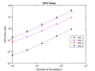
(a) CPU times in seconds.

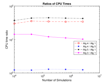
(b) Ratios CPU times

Table 1 reports the CPU times in seconds of all the approaches and compares the MC estimated values of the true $\bm{E}\left[{X(t)}\right]$, $\bm{V}\left[{X(t)}\right]$, $\bm{Skew}\left[{X(t)}\right]$ and $\bm{Kurt}\left[{X(t)}\right]$ at time $t=1/365$. Varying the number of simulations $N_{S}$, we can conclude that all the algorithms are equally convergent, although it seems that a large number of simulations is required to achieve a good estimate of the kurtosis. On the other hand, their computational performance is quite different. Figure 1(a) and 1(b) clearly show that Algorithm 1 by far outperforms all other approaches. It provides a remarkable improvement in terms of computational time that is at least $30$ times smaller than that of any other alternative available in the literature. With our computer generating $N_{S}=2560000$ values of $X(t)$ at time $t=1/365$ does not even take a second in contrast to several seconds using the other alternatives. Algorithm 3 is also faster than Algorithms 4 and Algorithm 5 although based on a acceptance-rejection method, but unfortunately, it is only applicable under the constraint $0.5\leq e^{-k\Delta t}<1$. To conclude, it seems that Algorithms 4 and Algorithm 5 exhibit similar CPU times.

Of course, the superior performances of Algorithm 1 with respect to all the alternatives becomes even more remarkable when the entire trajectory over a time grid is simulated. To this end, we generate the skeleton of the process on an equally space time grid $t_{1},\dots,t_{M}$ with $M=4$ and $\Delta t=1/4$. In order to better highlight the difference in performance among the approaches, we have here chosen the same parameter set as in Qu et al. [29], $(k,\lambda,\beta,x_{0})=(0.5,1,1,10)$.

The results in Table 2 confirm that our proposal provides the smallest CPU times making Algorithm 1 very attractive for real-time calculations. We remark that the CPU times in Table 2 are relative to the simulation of entire trajectory with four time steps while instead, the estimated statistics refer to the process at time $t=1$. Refining the time grid with a smaller time step will increase the overall computational times almost linearly making all alternatives to Algorithm 1 not competitive for real-time applications. It is also worthwhile noticing that our implementation, although based on a less powerful computer, returns smaller CPU times than those reported in Qu et al. [29] relative these authors’ approach. Finally, as described in Section 3, the simulation of a $\mathrm{bi}\Gamma$-OU process can be obtained by repeating the algorithms above two times therefore, we can extrapolate the same conclusions with regards to the $\mathrm{bi}\Gamma$-OU case.

We conclude this section illustrating the results of the numerical experiments relative to a symmetric $\mathrm{bi}\Gamma$-OU process where we have chosen the same set of parameters selected for the $\Gamma$-OUprocess. $\bm{E}\left[{X(t)}\right]=x_{0}e^{-kt}$ and the skewness is zero therefore in Table 1 we show the CPU times in seconds and the MC estimated values of the true $\bm{V}\left[{X(t)}\right]$ and $\bm{Kurt}\left[{X(t)}\right]$ at time $t=1/365$ only. We also remark that Algorithm 7 is also applicable because $\sqrt{2}/2\leq a<1$ using both parameter sets. The conclusions are very much in line with what found for a $\Gamma$-OU process. As expected, all the approaches are equally convergent and the CPU times are higher that those for the $\Gamma$-OU case because all the solutions require additional steps. From Figures 2(a) and 2(b) one can observe that Algorithm 6 is by far the fastest solution and Algorithm 7, even if based on an acceptance rejection method, is once more a faster solution than Algorithms 8 and Algorithm 9. On the other hand, these last two approaches seem to be equally fast with the former slightly outperforming the approach in Qu et al. adapted to the symmetric $\mathrm{bi}\Gamma$-OU process.

In Table 4 we also report the results of generating the trajectory of a symmetric $\mathrm{bi}\Gamma$-OU with the same parameters and time grid of the $\Gamma$-OU case. The values in Table 4 once more confirm that our newly developed simulation approach, detailed Algorithm 6, exhibits high accuracy as well as efficiency and in particular, largely outperforms any other alternative.

		$\bm{V}\left[{X(t)}\right]=0.0055$		$\bm{Kurt}\left[{X(t)}\right]=222.71$			$\bm{V}\left[{X(t)}\right]=0.0055$		$\bm{Kurt}\left[{X(t)}\right]=222.71$
	Algorithm 6					Algorithm 7
$N_{S}$	CPU	MC	error %	MC	error %	CPU	MC	error %	MC	error %
$10000$	$0.0034$	$0.0062$	$12.9$%	$141.39$	$34.8$%	$0.0837$	$0.0066$	$20.1$%	$218.45$	$0.8$%
$40000$	$0.0121$	$0.0055$	$0.97$%	$202.53$	$6.54$%	$0.1634$	$0.0057$	$2.96$%	$176.28$	$18.66$%
$160000$	$0.0559$	$0.0054$	$2.83$%	$207.09$	$4.44$%	$0.6415$	$0.0059$	$6.20$%	$227.93$	$5.18$%
$640000$	$0.2284$	$0.0054$	$2.35$%	$228.70$	$5.53$%	$2.3321$	$0.0057$	$2.79$%	$217.46$	$0.34$%
$2560000$	$0.9188$	$0.0055$	$1.15$%	$211.83$	$2.25$%	$9.2060$	$0.0055$	$0.39$%	$218.86$	$0.99$%
	Algorithm 8					Algorithm 9
$10000$	$0.15$	$0.0063$	$13.2$%	$266.74$	$23.1$%	$0.1915$	$0.0052$	$6.4$%	$190.45$	$12.1$%
$40000$	$0.56$	$0.0052$	$5.14$%	$203.09$	$6.28$%	$0.7769$	$0.0059$	$6.94$%	$212.10$	$2.13$%
$160000$	$2.24$	$0.0055$	$0.26$%	$246.67$	$13.82$%	$3.0793$	$0.0060$	$8.11$%	$223.25$	$3.02$%
$640000$	$8.98$	$0.0054$	$1.48$%	$216.01$	$0.32$%	$12.3615$	$0.0056$	$0.58$%	$224.35$	$3.06$%
$2560000$	$36.16$	$0.0055$	$0.54$%	$223.38$	$0.52$%	$49.8659$	$0.0055$	$0.31$%	$217.83$	$0.52$%

Table 3: CPU times in seconds and comparison among the true $\bm{V}\left[{X(t)}\right]$ and $\bm{Kurt}\left[{X(t)}\right]$ of a symmetric $\mathrm{bi}\Gamma$-OU process at time $t=1/365$ with $(k,\lambda,\beta,x_{0})=(36,10,3,0)$ and their relative estimated values with $N_{S}$ MC scenarios using Algorithms 6, 7, 8 and 9.

		$\bm{V}\left[{X(t)}\right]=1.2642$		$\bm{Kurt}\left[{X(t)}\right]=9.4919$			$\bm{V}\left[{X(t)}\right]=1.2642$		$\bm{Kurt}\left[{X(t)}\right]=9.4919$
	Algorithm 6					Algorithm 7
$N_{S}$	CPU	MC	error %	MC	error %	CPU	MC	error %	MC	error %
$10000$	$0.0157$	$1.2539$	$-0.82$%	$9.306$	$-1.99$%	$0.2502$	$1.2920$	$2.15$%	$8.966$	$-5.87$%
$40000$	$0.0193$	$1.2148$	$-4.07$%	$9.370$	$-1.31$%	$0.9680$	$1.2478$	$-1.32$%	$9.249$	$-2.62$%
$160000$	$0.1098$	$1.2598$	$-0.35$%	$9.498$	$0.06$%	$3.4811$	$1.2619$	$-0.19$%	$9.450$	$-0.44$%
$640000$	$0.4614$	$1.2617$	$-0.20$%	$9.509$	$0.18$%	$14.713$	$1.2576$	$-0.53$%	$9.536$	$0.47$%
$2560000$	$3.1008$	$1.2650$	$0.06$%	$9.537$	$0.47$%	$61.448$	$1.2648$	$0.05$%	$9.509$	$0.18$%
	Algorithm 8					Algorithm 9
$10000$	$0.6143$	$1.2844$	$1.6$%	$10.60$	$10.5$%	$0.7889$	$1.2325$	$-2.57$%	$8.222$	$-15.4$%
$40000$	$2.2989$	$1.2950$	$2.38$%	$9.668$	$1.83$%	$3.1908$	$1.2771$	$1.01$%	$9.168$	$-3.54$%
$160000$	$9.2519$	$1.2578$	$-0.51$%	$9.510$	$0.19$%	$12.327$	$1.2564$	$-0.63$%	$9.582$	$0.94$%
$640000$	$36.601$	$1.2617$	$-0.20$%	$9.579$	$0.91$%	$48.689$	$1.2622$	$-0.16$%	$9.422$	$-0.74$%
$2560000$	$147.79$	$1.2628$	$-0.12$%	$9.455$	$-0.39$%	$199.71$	$1.2651$	$0.06$%	$9.498$	$0.06$%

Table 4: CPU times in seconds and comparison among the true $\bm{V}\left[{X(t)}\right]$ and $\bm{Kurt}\left[{X(t)}\right]$ of a symmetric $\mathrm{bi}\Gamma$-OU process at time $t=1$ with $(k,\lambda,\beta,x_{0})=(0.5,1,1,10)$ and their relative estimated values with $N_{S}$ MC scenarios using Algorithms 6, 7, 8 and 9.

Figure 2: Symmetric $\mathrm{bi}\Gamma$-OU with $(k,\lambda,\beta,x_{0})=(36,10,3,0)$, $\Delta t=1/365.$

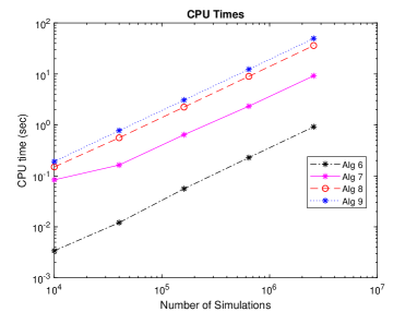
(a) CPU times in seconds.

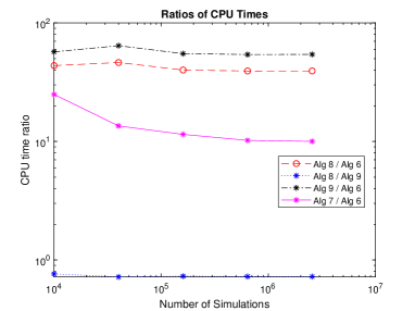
(b) Ratios CPU times

5 Conclusions and future inquiries

In this paper we have studied the distributional properties of the $\Gamma$-OU process and its bilateral counterpart $\mathrm{bi}\Gamma$-OU process. To this end, we have proven that in the transient regime the law of such processes is related to the law of the $a$-remainder of their relative sd stationary laws. Moreover, we have shown that the chf’s and the pdf’s of such laws can be represented in closed-form as a mixture of known and tractable laws, namely, a mixture of a Polya or a Binomial distribution.

As a simple consequence, we can design exact and efficient algorithms to generate the trajectory of a $\Gamma$-OU and a $\mathrm{bi}\Gamma$-OU process. Our numerical experiments have illustrated that our strategy has a remarkable computational advantage and cuts the simulation time down by a factor larger than $30$ compared to the existing alternatives available in the literature. In particular, due to the very small computational times, they are well suitable for real-time applications. One additional advantage is that our algorithms avoid the assumption of considering at most one jump per unit of time.

Moreover, although not the focus of our study, knowing the density in closed-form and having simple formulas for the cumulants of the distribution, one could conceive a parameter estimation procedure based on likelihood methods, on the generalized method of moments using the analogy with the GAR(1) auto-regressive processes introduced in Gaver and Lewis [16]. Of course, in any practical applications, some series truncation rule must be adopted as well as the generalization to time-dependent parameters is still open. These investigations will then be the focus of future inquires.

From the mathematical point of view, it would also be interesting to study if – and under which conditions – these results hold for other generalized Ornstein-Uhlenbeck processes: for instance, for processes whose stationary law is a Generalized Gamma Convolutions distribution (see Bondesson [7]) or for a Variance Gamma driven OU as discussed in Cummins et al.[12].

In a primarily economic and financial perspective, the future studies could cover the extension to a multidimensional setting with correlated Poisson processes as those introduced for instance in Lindskog and McNeil[23] or in Cufaro Petroni and Sabino [11]. A last topic deserving further investigation is the time-reversal simulation of the $\Gamma$-OU and $\mathrm{bi}\Gamma$-OU processes generalizing the results of Pellegrino and Sabino[27] and Sabino[30] to the case of the mean reverting compound Poisson processes.

References

• [1] L. Barabesi and L. Pratelli. A note on a Universal Random Variate Generator for Integer-valued Random Variables. Statistics and Computing, 24(4):589–596, 2014.
• [2] O.E. Barndorff-Nielsen and N. Shephard. Non-Gaussian Ornstein-Uhlenbeck-based models and some of their uses in financial economics. Journal of the Royal Statistical Society: Series B, 63(2):167–241, 2001.
• [3] F.E. Benth and A. Pircalabu. A non-gaussian ornstein-uhlenbeck model for pricing wind power futures. Applied Mathematical Finance, 25(1), 2018.
• [4] M.L. Bianchi and F.J. Fabozzi. Investigating the Performance of Non-Gaussian Stochastic Intensity Models in the Calibration of Credit Default Swap Spreads. Computational Economics, 46(2):243–273, Aug 2015.
• [5] M.L. Bianchi and G.L. Tassinari. Forward-looking Portfolio Selection with Multivariate Non- Gaussian Models and the Esscher Transform. arXiv preprint:1805.05584, 2018.
• [6] A. Bignami and A. de Matteis. A Note on Sampling from Combination of Distribution. Journal of the Institute of Mathematics and its Applications, 8:80–81, 1971.
• [7] L. Bondesson. Generalized Gamma Convolutions. Springer New York, New York, NY, 1992.
• [8] A. Cartea and M. Figueroa. Pricing in Electricity Markets: a Mean Reverting Jump Diffusion Model with Seasonality. Applied Mathematical Finance, No. 4, December 2005, 12(4):313–335, 2005.
• [9] R. Cont and P. Tankov. Financial Modelling with Jump Processes. Chapman and Hall, 2004.
• [10] N. Cufaro-Petroni. Self-decomposability and Self-similarity: a Concise Primer. Physica A, Statistical Mechanics and its Applications, 387(7-9):1875–1894, 2008.
• [11] N. Cufaro-Petroni and P. Sabino. Coupling Poisson Processes by Self-decomposability. Mediterranean Journal of Mathematics, 14(2):69, 2017.
• [12] M. Cummins, G. Kiely, and B. Murphy. Gas Storage Valuation under Lévy Processes using Fast Fourier Transform. Journal of Energy Markets, 4:43–86, 2017.
• [13] A. Dassios and J. Jang. Pricing of Catastrophe Reinsurance and Derivatives Using the Cox Process with Shot Noise Intensity. Finance and Stochastics, 7(1):73–93, 2003.
• [14] L. Devroye. On the Computer Generation of Random Variables with a given Characteristic Function. Computers & Mathematics with Applications, 7(6):547–552, 1981.
• [15] L. Devroye. Non-Uniform Random Variate Generation. Springer-Verlag, 1986.
• [16] D. P. Gaver and P. A. W. Lewis. First-order Autoregressive Gamma Sequences and Point Processes. Advances in Applied Probability, 12(3):727–745, 1980.
• [17] B. Grigelionis. On the Self-Decomposability of Euler’s Gamma Function. Lithuanian Mathematical Journal, 43(3):295–305, 2003.
• [18] M. Kjaer. Pricing of Swing Options in a Mean Reverting Model with Jumps. Applied Mathematical Finance, 15(5-6):479–502, 2008.
• [19] T. Kluge. Pricing Swing Options and other Electricity Derivatives. Technical report, University of Oxford, 2006. PhD Thesis, Available at http://perso-math.univ-mlv.fr/users/bally.vlad/publications.html.
• [20] S. G. Kou. A Jump-Diffusion Model for Option Pricing. Manage. Sci., 48(8):1086–1101, August 2002.
• [21] U. Küchler and S. Tappe. Bilateral Gamma Distributions and Processes in Financial Mathematics. Stochastic Processes and their Applications, 118(2):261–283, 2008.
• [22] A.J Lawrance. The Innovation Distribution of a Gamma Distributed Autoregressive Process. Scandinavian Journal of Statistics, 9:234–236, 1982.
• [23] F. Lindskog and J. McNeil. Common poisson shock models: applications to insurance and credit risk modelling. ASTIN Bulletin, 33(2):209–238, 2003.
• [24] E. McKenzie. Innovation Distridution for Gamma and Negative Binomial Autoregressions. Scandinavian Journal of Statistics: Theory and Applications, 14(1):79–85, 1987.
• [25] T. Meyer-Brandis and P. Tankov. Multi-factor Jump-diffusion Models of Electricity Prices. International Journal of Theoretical and Applied Finance, 11(5):503–528, 2008.
• [26] H.H. Panjer and G.E. Willmot. Finite sum evaluation of the negative binomial-exponential model. ASTIN Bulletin, 12(2):133–137, 1981.
• [27] T. Pellegrino and P. Sabino. Enhancing least squares monte carlo with diffusion bridges: an application to energy facilities. Quantitative Finance, 15(5):761–772, 2015.
• [28] G. Popovici and M. Dumitrescu. Estimation on a GAR(1) Process by the EM Algorithm. Economic Quality Control, 22(2):165–174, 2010.
• [29] Y. Qu, A. Dassios, and H. Zhao. Exact Simulation of Gamma-driven Ornstein–Uhlenbeck Processes with Finite and Infinite Activity Jumps. Journal of the Operational Research Society, 0(0):1–14, 2019.
• [30] P. Sabino. Forward or Backward Simulations? A Comparative Study. Quantitative Finance, 2020. In press.
• [31] K. Sato. Lévy Processes and Infinitely Divisible Distributions. Cambridge U.P., Cambridge, 1999.
• [32] W. Schoutens. Lévy Processes in Finance: Pricing Financial Derivatives. John Wiley and Sons Inc, 2003.
• [33] W. Schoutens and J. Cariboni. Lévy Processes in Credit Risk. John Wiley and Sons, Chichester., 2010.
• [34] M.K. Simon. Probability Distributions Involving Gaussian Random Variables. The Springer International Series in Engineering and Computer Science, 2006.