On multiple SLE for the FK–Ising model

Abstract.

We prove convergence of multiple interfaces in the critical planar $q=2$ random cluster model, and provide an explicit description of the scaling limit. Remarkably, the expression for the partition function of the resulting multiple SLE_16/3 coincides with the bulk spin correlation in the critical Ising model in the half-plane, after formally replacing a position of each spin and its complex conjugate with a pair of points on the real line. As a corollary, we recover Belavin–Polyakov–Zamolodchikov equations for the spin correlations.

1. Introduction

Schramm–Loewner evolution [49] provides a geometric description of scaling limits of critical planar models of statistical mechanics. Its importance stems for the fact that SLE is characterized by two simple properties, namely, the conformal invariance and the domain Markov property. When the random curve in question is described by Loewner evolution, these two properties imply that the driving process has independent, identically distributed increments. Since it is continuous, this identifies it as a Brownian motion with a constant drift; mild additional symmetries such as scaling outrule the latter.

This simple characterization requires the boundary conditions to be sufficiently simple, so that any domain (in particular, the domain slit by the initial segment of the curve) can be conformaly mapped onto any other domain in such a way that the boundary conditions match. This can be achieved when there are no more than three “marked points” on the boundary (i. e., points where boundary conditions change), or one on the boundary and one in the bulk. Examples include a single loop-erased random walk curve with Dirichlet boundary conditions [46], harmonic explorer [50] and the level lines of the Gaussian Free Field [51] with jump boundary condtitions, Dobrushin [10] and plus/minus/free [28, 29] boundary conditions in the Ising model and wired/free boundary conditions in the FK–Ising model [10]. These exmaples lead to chordal, radial or dipolar SLE.

When the boundary conditions are more complicated, additional insight is needed to characterize possible laws of the driving process. On the physical level of rigor, it is clear that the law of the initial segments of the curves should be absolutely continuous under the change of boundary conditions far away. Hence, in general, the law of the driving process should be given by a Brownian motion with a (time-dependent) drift. Moreover, the Radon-Nikodym derivative with respect to an interface with simpler (e. g., Dobrushin-type) boundary conditions can be written as a ratio of partition functions, from which the drift term can be derived by Girsanov transform. This led Bauer, Bernard, and Kytölä [1] to a conjecture that to each boundary conditions in a simply-connected domain $\Omega,$ one can associate an SLE partition function $Z(b^{(1)},\dots,b^{(n)})$, $b^{(1)},\dots,b^{(n)}\in\mathbb{R},$ so that the driving process $b_{t}^{(1)}$ describing the curve $\gamma_{t}$ starting form $b^{(1)}$ satisfies the SDE

$$db_{t}^{(1)}=\sqrt{\kappa}dB_{t}+\kappa\partial_{b^{(1)}}\log Z(b_{t}^{(1)},\dots,b_{t}^{(n)})dt,$$

where $b_{t}^{(i)}=g_{t}(\varphi(b^{(i)}))$ for $i\geq 2$, $g_{t}$ are the Loewner maps, $\varphi$ is a conformal map from $\Omega$ to the upper half-plane $\mathbb{H}$, and $b^{(i)}\in\partial\Omega$ are the marked points for the boundary conditions in question. Moreover, since $Z(b_{t}^{(1)},\dots,b_{t}^{(n)})$ can be identified with a “boundary change operator” correlation in the corresponding conformal field theory, the function $Z$ was conjectured to satisfy a system of second order partial differential equations known as Belavin–Polyakov–Zamolodchikov (BPZ) equations in Conformal Field Theory [4]. Alternatively, these equations can be derived from the fact that since $Z(b_{t}^{(1)},\dots,b_{t}^{(n)})$ is supposed to be a Radon–Nikodym derivative with respect to a chordal SLE, it should be a (conformally covariant) chordal SLE martingale.

Making this reasoning rigorous is hard, since it requires controlling the scaling limits of partition functions, in particular, in rough domains. However, it was discovered by Dubédat [15] and independently by Zhan [56] that if each of the marked points $b^{(1)},\dots,b^{(n)}$ has its own SLE-like interface growing from it, then natural consistency conditions, or “commutation relations”, actually imply the existence of an SLE partition function with the above properties.

Recently, a lot of progress has been made in finding relevant solutions to the BPZ equations, or proving that the solutions with required properties are unique. The upshot of these results is that for $2n$ marked points on the boundary, any multiple SLE is a mixture of one of $\frac{(2n)!}{n!(n+1)!}$ pure geometry multiple SLE, i. e., the ones where marked points are connected to each other in a prescribed planar pattern. The relevant description was proven by Flores and Kleban in [19, 20, 21, 22]. Independently, Kytölä and Peltola [45, 44] have given explicit expressions for the partition function of pure geometry multiple SLE in terms of Coulomb gas integrals for all $\kappa\notin\mathbb{Q}$. The restriction to $\kappa\notin\mathbb{Q}$ is due to the fact that representation theory of the quantum group $\mathcal{U}_{q}(su_{2})$, $q=e^{4\pi i/\kappa}$ is used in the construction, and this theory is much more intricate for $q$ a root of unity.

An independent line of study, started by Lawler and Kozdron [43], bypasses completely the theory of BPZ equations. Instead, it purports to construct pure geometry multiple SLE using Brownian loop measures, and then to prove that there is at most one process satisfying a natural set of axioms. This program has been recently completed by Beffara, Peltola and Wu [3] in the case $\kappa\in(0;4]$. For $\kappa\in(4;6]$, they got a corresponding result conditionally on convergence of single interface in the corresponding random-cluster model. In particular, since this convergence was established for $\kappa=\frac{16}{3}$, their result implies convergence of multiple interfaces in the FK model, conditioned on the connection geometry. Their result does not yield explicit description of the law of the curves.

The above results mostly concern the pure geometry case. On the other hand, in the underlying lattice model, there is usually a natural “physical” measure on the interfaces, without restrictions on how they connect to each other. The corresponding multiple SLE partition function (sometimes called the full partition function) can, in principle, be found by analysis of the space of solution to BPZ equations; however, deriving explicit expressions at rational $\kappa$ by this method is difficult. When the convergence of interfaces is known, usually integrability features of the model allow one to derive explicit solution for the “physical” multiple SLE, as follows:

• In the critical Ising model with alternating $+/-/\dots+/-$ boundary conditions, the interfaces converge [30, 47] to multiple SLE₃ with partition function

  $$Z(b^{(1)},\dots,b^{(2n)})=\mathrm{Pf}\left[(b^{(i)}-b^{(j)})^{-1}\right].$$

  The Pfaffian structure of the partition function is due to the fact that boundary condition change can be achieved by placing a fermion on the boundary. In [29], this has been extended to allow free boundary arcs, in which case there is no simple Pfaffian structure. For the the multiply-connected case, see [30].

• In the Gaussian free field with alternating $+\lambda/-\lambda/\dots/+\lambda/-\lambda$ boundary conditions, the level lines are multiple SLE₄ with the partition function

  $$Z(b^{(1)},\dots,b^{(2n)})=\prod_{i<j}(b^{(i)}-b^{(j)})^{\frac{1}{2}(-1)^{i-j}};$$

  which is in fact also the partition function of the underlying GFF [16, 48]. See also [27, 31] for the doubly-connected case.

• The branches between $2n$ boundary points in Uniform spanning tree with wired boundary conditions converge to multiple SLE₂ with partition function

  $$Z(b^{(1)},\dots,b^{(2n)})=\sum_{\omega}\mathrm{sgn}(\omega)\det\left[(b^{(i)}-b^{\omega(j)})^{-2}\right]_{i<\omega(i);j<\omega(j)}$$

  where the sum is over all involutions $\omega:\{1,\dots,2n\}\to\{1,\dots,2n\}$ without fixed points [36, 37, 35]. The structure of the partition function is related to the determinantal nature of the UST and the Fomin identity [23].

The main contribution of this paper is the corresponding result for the FK–Ising model.

Theorem 1.1.

The interfaces in the critical FK–Ising model with free boundary conditions on $(b^{(1)},b^{(2)})$, $(b^{(3)},b^{(4)})$, $\dots,$ $(b^{(2n-1)},b^{(2n)})$ and wired boundary conditions on $(b^{(2)},b^{(3)}),$ $(b^{(4)},b^{(5)})$, $\dots$, $(b^{(2n)},b^{(1)})$ converge to multiple SLE_16/3 with partition function

(1.1) $$Z(b^{(1)},\dots,b^{(2n)})=\prod_{k=1}^{n}(b^{(2k)}-b^{(2k-1)})^{-\frac{1}{8}}\left(\sum_{\sigma\in\{\pm 1\}^{n}}\prod_{i<j}\chi_{ij}^{\frac{\sigma_{i}\sigma_{j}}{4}}\right)^{\frac{1}{2}},$$

where $\chi_{ij}=\frac{(b_{2i}-b_{2j})(b_{2i-1}-b_{2j-1})}{(b_{2i}-b_{2j-1})(b_{2i-1}-b_{2j})}.$

The mode of convergence is that the collections of full curves converge to the corresponding global multiple SLE, see Definition 5.7. The technicalities are by now quite standard in the one-curve case, where precompactness and similar issues have been resolved by Kemppainen and Smirnov [39]. The multi-curve case they has been recently systematically treated by Karrila [34], who takes RSW-type bounds and the convergence in the mode of Lemma 5.2 below as inputs and explores conclusions. We use some of his arguments, but our exposition is self-contained, only relying on [39].

The result of Theorem 1.1 was conjectured by Flores, Simmons, Kleban and Ziff [52]. Their conjecture was based on the observation that the expression in (1.1) formally coincides with the bulk spin correlation function in the Ising model on the upper half-plane when each pair of real numbers $b^{(2i-1)},b^{(2i)}\in\mathbb{R}$ is replaced with a pair of complex conjugates $a_{i},\bar{a}_{i}$. Since the spin correlations are believed to satisfy the BPZ equations, so should (1.1). The spin correlations were rigorously computed in [12]; however, the author is not aware of a published proof that they do indeed satisfy the BPZ equations (although the result was announced in [5]). We can actually derive this result from Theorem 1.1 and Dubédat’s commuting SLE theory:

Corollary 1.2.

The spin correlations in the scaling limit of the critical Ising model in the half-plane, given by the formula

$$\prod_{k=1}^{n}(\Im\mathfrak{m}a_{i})^{-\frac{1}{8}}\left(\sum_{\sigma\in\{\pm 1\}^{n}}\prod_{i<j}\left|\frac{a_{i}-a_{j}}{a_{i}-\bar{a}_{j}}\right|^{\frac{\sigma_{i}\sigma_{j}}{2}}\right)^{\frac{1}{2}}$$

satisfy the BPZ equations; namely, for each $i=1,\dots,n$, they are annihilated by

(1.2) $$\frac{8}{3}\frac{\partial^{2}}{(\partial a_{i})^{2}}+\sum_{j\neq i}\frac{2}{a_{j}-a_{i}}\frac{\partial}{\partial a_{j}}+\sum\frac{2}{\bar{a}_{j}-a_{i}}\frac{\partial}{\partial\bar{a}_{j}}+\sum_{j\neq i}\frac{1/8}{(a_{j}-a_{i})^{2}}+\sum\frac{1/8}{(\bar{a}_{j}-a_{i})^{2}}.$$

Proof.

The scaling limit of FK–Ising interfaces is, by construction, a family of commuting SLE. By Dubédat’s commutation relations [15], see [25, Section 5, in particular (5.47)] for an explicit treatment, multiple SLE_16/3 partition function (1.1) (which is determined uniquely up to a multiplicative constant by its logarithmic derivatives, and thus by the law of the curves) satisfies these equations with $(a_{i},\bar{a}_{i})$ replaced by $(b_{2i-1};b_{2i}).$ The result follows. ∎

The result of Theorem 1.1 for $n=1$ was established in [10], relying on the breakthrough proof by Smirnov [54, 53, 14] of conformal invariance of fermionic observable, combined with the precompactness results of [39] and Russo-Seymour-Welsh bounds [17, 9]; see also [42] for the doubly connected case. For $n=2$, the main ingredient was obtained in [14], where convergence of the martingale observable was proven, and the details for the convergence of interfaces were given in [40]. These results were later used to describe full scaling limit of the loop representation of the FK–Ising model [41, 38].

In this paper, for simplicity, we work exclusively with the square lattice. The results can be readily extended to isoradial setup by the techniques of [14]; recently, Chelkak has proven the one-curve convergence result in a fully universal setup via s-embeddings [6, 13, 7]. Eventually, it should be possible to derive the result of the present paper in the same generality.

The “wired” boundary arcs in Theorem 1.1 are meant to be wired altogether. Another natural setup, where they are wired, but not wired to each other, is actually dual to this one, so we do not need to consider it separately. It would be natural to consider other external connections between the wired arcs. Given such a connection, the Radon–Nikodym derivative of the corresponding multiple SLE with respect to the one considered in Theorem 1.1 is simply a function of connection pattern of the multiple interfaces inside the domain. Hence, calculating the law of the curves in this situation is essentially equivalent to computing the probabilities of all $\frac{(2n)!}{n!(n+1)!}$ connection patterns. While we are at the moment unable to give explicit expressions for these probabilities, the convergence of the interfaces implies conformal invariance.

Corollary 1.3.

Let $\Omega^{\delta}$ be discrete domains with $2n$ marked boundary points $b^{(1,\delta)},\dots,b^{(2n,\delta)}$. Let $\pi$ be a partition of the set $(b^{(2,\delta)},b^{(3,\delta)}),(b^{(4,\delta)},b^{(5,\delta)}),\dots$ of wired boundary arcs. Consider the critical FK–Ising model in $\Omega^{\delta}$ with boundary conditions as in Theorem 1.1, and let $\pi^{\delta}$ be the random partition of the set of wired boundary arcs induced by the random clusters inside $\Omega^{\delta}$. Then, for each $\pi$, the quantity $\mathsf{\mathbb{P}}(\pi^{\delta}=\pi)$ has a conformally invariant scaling limit.

In [29], it was noted that probabilities of a number of connection events can be computed directly as special values discrete holomorphic observables. This leads to a proof of their convergence and conformal invariance in the scaling limit that completely bypasses the SLE theory. In the half-plane, the expression for the scaling limits are explicit quadratic irrational functions. The class of these events was, however, described in [29] incorrectly. In fact, there are $2^{n-1}-1$ such non-trivial events, one for each non-empty subset $S$ of the set of free boundary arcs with $|S|$ even. The event corresponding to $S$ can be described as “no dual cluster touches an odd number of arcs in $S$”. The explicit expression are given by the ratios of the half-plane spin-disorder correlations to spin correlations, with the familiar replacement $(a_{i},\bar{a}_{i})\to(b_{2i-1};b_{2i})$ and the disorders corresponding to arcs in $S$, see further details in [11].

In particular, when $|S|=2$, this is just the probability that two wired arcs are connected, generalizing a result from [14]. We do not know whether all connection probabilities, or even any connection probabilities other than just described, are given by quadratic irrational functions.

The paper is organized as follows. In Section 2, we introduce the graph notation and define the model. In Section 3, we recall the definition of a discrete holomorphic observable and the convergence result from [29], and show that this observable also possesses a martingale property with respect to the FK–Ising interface. In Section 4, we prove tightness of the interfaces and show that the scaling limit of the martingale observable is a martingale with respect to any sub-sequential scaling limit of the interfaces. In Section 5, we prove Theorem 1.1. The main idea of the derivation of the law of the driving process (up to disconnection threshold) from the martingale observable is as in [57, 31, 30], and is based on the expansion of the martingale observable at the tip of the curve. The version of this argument presented here uses contour integration and is significantly shorter as compared to [30]; of a separate interest is a short proof of Lemma 5.1 showing that the driving process is a semi-martingale. After deriving the convergence in a “local” mode, an easy application of the RSW results of [9] shows that if the discrete interface almost disconnects the domain, then, with high probability, it actually does disconnect it quickly and with “nothing interesting” happening in between. This allows to conclude the proof by induction.

The author is grateful to Alex Karrila, Eveliina Peltola and Hao Wu for stimulating discussions.

2. The FK–Ising model

We denote $\mathbb{C}^{\delta}:=\delta\mathbb{Z}^{2}$, and $\mathbb{C}^{\delta,\bullet}:=\delta\mathbb{Z}^{2}+\frac{\delta}{2}+\frac{i\delta}{2}$, the square lattice of mesh size $\delta$ and its dual, respectively. By a simply connected discrete domain $\Omega^{\delta}$ we mean a domain whose boundary $\partial\Omega^{\delta}$ is a simple nearest-neighbor closed path in $\mathbb{C}^{\delta,\bullet}$. We denote by $\mathcal{E}(\Omega^{\delta})$ and $\mathcal{V}(\Omega^{\delta})$ the sets of edges and vertices of $\mathbb{C}^{\delta}$ that lie in $\Omega^{\delta}$, respectively.

The alternating wired/free boundary conditions $\mathcal{\beta}^{\delta}$ for a simply-connected domain $\Omega^{\delta}$ are specified by a partition of $\partial\Omega^{\delta}$ into a “wired” part $\mathcal{\beta}_{\mathrm{wired}}^{\delta}:=\beta_{2}^{\delta}\cup\dots\cup\beta_{2n}^{\delta}$ and a free part $\mathcal{\beta}_{\mathcal{\mathrm{free}}}^{\delta}=\beta_{1}^{\delta}\cup\dots\cup\beta_{2n-1}^{\delta}$, where $\mathcal{\beta}_{i}^{\delta}=(b^{(i,\delta)};b^{(i+1,\delta)})$ are boundary arcs, and $b^{(2n+1,\delta)}=b^{(1,\delta)},\dots,b^{(2n,\delta)}\in\partial\Omega^{\delta}\cap\mathcal{V}(\mathbb{C}^{\delta,\bullet})$ are boundary points separating the arcs, in counterclockwise order. Put

$$\hat{\mathcal{E}}(\Omega^{\delta})=\mathcal{E}(\Omega^{\delta})\cup\{e\in\mathcal{E}(\mathbb{C}^{\delta}):e\cap\mathcal{\beta}_{\mathrm{wired}}^{\delta}\neq\emptyset\},$$

the set of edges of $\mathbb{C}^{\delta}$ that either belong to $\Omega^{\delta}$, of cross the “wired” part of the boundary.

The main subject of this paper is the critical planar $q=2$ Fortuin–Kasteleyn random cluster model, or FK–Ising model [24, 26]. This is a random collection $E\subset\hat{\mathcal{E}}(\Omega^{\delta})$ of edges chosen according to the probability measure

$$\mathsf{\mathbb{P}}_{\Omega^{\delta},\mathcal{\beta}^{\delta}}(E)=\frac{1}{Z_{\text{FK}}}\left(\frac{p}{1-p}\right)^{|E|}2^{\mathcal{C}(E)}.$$

Here $\mathcal{C}(E)$ is the number of clusters (connected components) in $E$, where all vertices outside of $\Omega^{\delta}$ are considered to belong to the same cluster, and

$$Z_{\text{FK}}=\sum_{E}p^{|E|}(1-p)^{-|E|}2^{\mathcal{C}(E)}$$

is the partition function.

Given $e\in\mathcal{E}(\mathbb{C}^{\delta})$, its dual edge $e^{\bullet}\in\mathcal{E}(\mathbb{C}^{\delta,\bullet})$ is the edge of the dual lattice that crosses $e.$ Given a configuration $E\subset\mathcal{E}(\Omega^{\delta})$, we define its dual configuration $E^{\bullet}\subset\mathcal{E}(\mathbb{C}^{\delta,\bullet})$ by

$$E^{\bullet}:=\{e^{\bullet}:\left(e\in\mathcal{E}(\Omega^{\delta})\text{ or }e\cap\partial\Omega^{\delta}\neq\emptyset\right)\text{ and }\,e\notin E\}.$$

Note that it particular, $E^{\bullet}$ always contains all the edges comprising $\mathcal{\beta}_{\mathcal{\mathrm{free}}}^{\delta}$. It is not hard to see that adding an edge to $E$ either disconnects two clusters of $E^{\bullet}$, or connects two clusters of $E$, but never both. Hence, $\mathcal{C}(E^{\bullet})+|E^{\bullet}|-\mathcal{C}(E)$ does not, in fact, depend on $E$, and the probability of the configuration can be also written as

$$\mathsf{\mathbb{P}}_{\Omega^{\delta},\mathcal{\beta}^{\delta}}(E)=\frac{1}{Z_{\text{FK}}^{\bullet}}\left(\frac{2(1-p)}{p}\right)^{|E^{\bullet}|}2^{\mathcal{C}(E^{\bullet})}.$$

The self-dual point of the model, given by the condition $p/(1-p)=2(1-p)/p$, is also known to be its critical point; this result in fact holds for any $q\geq 1$ [2]. For the rest of the paper, we set $p$ to its critical value $p_{c}=2-\sqrt{2}$.

Note that in $E^{\bullet}$, the arcs $\beta_{1}^{\delta},\dots,\beta_{2n-1}^{\delta}$ are wired, but not wired together, which is the duality mentioned in the introduction.

The medial lattice $\mathcal{M}(\mathbb{C}^{\delta})$ is the square lattice whose vertices are the midpoints of edges of $\mathbb{C}^{\delta}$. Given a configuration $E$, an exploration interface is a nearest-neighbor path on $\mathcal{M}(\mathbb{C}^{\delta})$ that turns by $\pm\frac{\pi}{2}$ at every step, and never crosses edges of either $E$, or $E^{\bullet}$, or $\mathcal{E}$($\mathbb{C}^{\delta}$$\setminus\Omega^{\delta}$), transversally, see Figure 2.1. An exploration interface $\gamma$ is completely determined by its starting (oriented) edge and the configuration $E$; in its turn, its initial segment determines the state of all edges whose midpoints it has visited, except possibly for the last one.

We will be interested in the statistics of the interface $\gamma^{\delta}=(\gamma_{0}^{\delta},\gamma_{1}^{\delta},\dots)$ starting in between $\beta_{\mathrm{wired}}^{\delta}$ and $\beta_{\mathcal{\mathrm{free}}}^{\delta}$, say at $b^{(1,\delta)}$. More precisely, we let $\gamma_{0}^{\delta}$ be an oriented edge of $\mathcal{M}(\mathbb{C}^{\delta})$ that has $b^{(1,\delta)}$ on its right and a vertex of $\mathbb{C}^{\delta}\setminus\Omega^{\delta}$ on its left. We say the an edge of $\hat{\mathcal{E}}(\Omega^{\delta})$ is revealed by $\gamma_{[0,t]}^{\delta}$ if its midpoint is an endpoint of one of the edges $\gamma_{0}^{\delta},\dots,\gamma_{t-1}^{\delta}.$ By induction, the medial edge $\gamma_{t}^{\delta}$ will always have on its right a dual vertex connected to $\beta_{1}^{\delta}$ by a sequence of edges of $E^{\bullet}$ revealed by $\gamma_{[0,t]}^{\delta}$, and on its left a primal vertex connected to $\mathbb{C}^{\delta}\setminus\Omega^{\delta}$ by a sequence of edges of $E$ revealed by $\gamma_{[0,t]}^{\delta}$.

By $\Omega^{\delta}_{t},$ we denote the (random) domain obtained by removing from $\Omega^{\delta}$ all the vertices that are incident to the edges of $E$ revealed by $\gamma^{\delta}$ by time $t$. Although $\Omega^{\delta}_{t}$ is not necessarily connected, each of its connected components is simply connected. The domain $\Omega^{\delta}_{t}$ is naturally equipped with the boundary conditions $\mathcal{\beta}_{t}^{\delta}$ that are free on $\mathcal{\beta}_{\mathcal{\mathrm{free}}}^{\delta}$ and on all dual edges revealed to be in $E^{\bullet}$ by time $t$, and wired elsewhere. As long as $b^{(2,\delta)},\dots,b^{(2n,\delta)}$ are on the boundary of the same connected component of $\Omega^{\delta}_{t}$, on that component $\mathcal{\beta}_{t}^{\delta}$ are specified by $2n$ arcs, with the additional marked points separating the free boundary arc adjacent to $b^{(2,\delta)}$ and the wired boundary arc adjacent to $b^{(2n,\delta)}.$ The conditional law of $E$ given $\gamma_{[0,t]}^{\delta}$ is the union of the edges of $E$ revealed by time $t$ and a critical FK–Ising configuration in $\Omega_{t}^{\delta}$ with boundary conditions $\mathcal{\beta}_{t}^{\delta}$. This property is clear from the definition and is an instance of the domain Markov property.

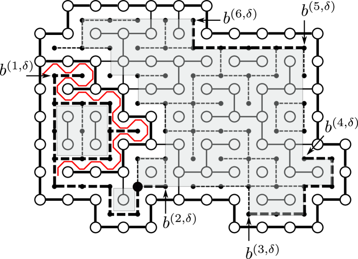
Figure 2.1. An example of a discrete domain $\Omega^{\delta}$ with six marked boundary points, a configuration $E$ (solid edges connecting the $\circ$ vertices of $\mathbb{C}^{\delta}$) and $E^{\bullet}$ (dashed edges connecting the $\bullet$ vertices of $\mathbb{C}^{\delta,\bullet}$). The vertices of the exterior loop formed by solid edges belong to $\mathbb{C}^{\delta}\setminus\Omega^{\delta}$ and are thus wired altogether. An initial segment $\gamma_{[0,t]}^{\delta}$ of the interface starting from $b^{(1,\delta)},$ for $t=24,$ is drawn in red. Bold edges and dual edges are discovered by the interface, or their state is prescribed by boundary conditions. The state of thin edges given $\gamma_{[0,t]}^{\delta}$ is genuinely random. In gray is the domain $\Omega^{\delta}_{t}$, which consists of three connected components. One of them has on its boundary $b^{(2,\delta)},\dots,b^{(2n,\delta)}$ and exactly one additional marked boundary point, the big black dot.

3. The martingale observable

In this section, we recall from [29] the definition of a discrete holomorphic observable that has been used to derive convergence of multiple interfaces in the spin Ising model in the presence of free boundary arcs. It turns out that the same observable possesses a martingale property with respect to the FK interface. The observable was given in [29] in terms of the low-temperature expansion. The proof of its martingale property consists of first writing it in the order-disorder formalism of Kadanoff–Ceva [32], see also [8, 11], and then invoking Edwards–Sokal coupling [18, 26] and the domain Markov property.

For a discrete domain $\Omega^{\delta}$, denote by $\Omega^{\delta,\bullet}:=\mathbb{C}^{\delta,\bullet}\cap\left(\Omega^{\delta}\cup\partial\Omega^{\delta}\right)$ its dual domain. Let $a,z$ be two corners in $\Omega^{\delta}$ or adjacent to its boundary, i. e., two midpoints of segments ($a^{\bullet}a^{\circ}$) and $(z^{\bullet}z^{\circ})$ connecting vertices $a^{\circ},z^{\circ}\in\mathcal{V}(\mathbb{C}^{\delta})$ with adjacent dual vertices $a^{\bullet},z^{\bullet}\in\Omega^{\delta,\bullet}$. We denote by $\mathrm{Conf}_{\Omega^{\delta}}$ the set of all subsets $S\subset\mathcal{E}(\Omega^{\delta,\bullet})$ such that all vertices of $\Omega^{\delta,\bullet}$ have even degree in $S$, and by $\mathrm{Conf}_{\Omega^{\delta}}(a,z)$ the set of all subsets $S\subset\mathcal{E}(\Omega^{\delta,\bullet})$ such that all such that all vertices of $\Omega^{\delta,\bullet}$ have even degree in $S$, except for $a^{\bullet},z^{\bullet}$ that have odd degree in $S$. The winding $\mathrm{wind}(S)$ is defined by the following procedure: add to $S$ the segments $(a,a^{\bullet})$ and $(z^{\bullet},z)$, and decompose the resulting graph into a collection of loops and a path $S^{\prime}$ connecting $a$ and $z$, in such a way that the loops and the path do not intersect themselves or each other transversally. (This amounts to resolving each vertex of degree four in one of the two possible ways.) Then, the winding number of $S^{\prime}$ (i. e., the rotation number of its tangent vector) does not depend on the decomposition, and that is defined to be $\mathrm{wind}(S).$

Definition 3.1.

([29], Section 2, case $m=0$, $s=2$) Let $(\Omega^{\delta},\mathcal{\beta}^{\delta})$ be a discrete simply connected domain, and let $a\notin\text{$\Omega^{\delta}$}$ be a marked corner such that $a^{\bullet}\in\partial\Omega^{\delta}$ separates $\beta_{\mathrm{wired}}^{\delta}$ from $\beta_{\mathcal{\mathrm{free}}}^{\delta}$. The fermionic observable is defined by

$$F_{\Omega^{\delta},\mathcal{\beta}^{\delta}}(z)=\mathfrak{i}\eta_{a}\cdot\frac{\sum_{S\in\mathrm{Conf}_{\Omega^{\delta}}(a,z)}e^{-\frac{\mathfrak{i}}{2}\mathrm{wind}(S)}\alpha^{|S\setminus\beta_{\mathcal{\mathrm{free}}}^{\delta}|}.}{\sum_{S\in\mathrm{Conf}_{\Omega^{\delta}}}\alpha^{|S\setminus\beta_{\mathcal{\mathrm{free}}}^{\delta}|}.},\quad\alpha:=\sqrt{2}-1,$$

where $\eta_{a}:=\left(\frac{a-a^{\bullet}}{|a-a^{\bullet}|}\right)^{-\frac{1}{2}}.$

Remark 3.2.

The observable $F_{\Omega^{\delta},\mathcal{\beta}^{\delta}}(z)$ depends on the choice of the square root in the definition of $\eta_{a}$. If a family of simply-connected domains all have common part of the boundary, as will be the case with domains $\Omega^{\delta}_{t},$ then such a choice can be made coherently by fixing the sign of the square root of the outer normal at some point of the common boundary and then extending it continuously, say, in counterclockwise direction. With this convention, $F_{\Omega^{\delta},\mathcal{\beta}^{\delta}}$ depends only on $a^{\bullet}$ but not on the choice of the corner $a$ adjacent to it. We incorporate the choice of $a^{\bullet}$ into the boundary conditions $\mathcal{\beta}^{\delta}$ and do not stress it separately in the notation.

Lemma 3.3.

For any corner $z\in\Omega^{\delta}$, the sequence

$$F_{\Omega^{\delta}_{t},\mathcal{\beta}_{t}^{\delta}}(z)$$

is a martingale with respect to the filtration $\mathcal{F}_{t}:=\sigma(\gamma_{[0,t]})$, as long as $z$ is in the same connected component of $\Omega^{\delta}_{t}$ as $b^{(2,\delta)},\dots,b^{(2n,\delta)}$

Proof.

Recall the Edwards–Sokal coupling: one samples $E\subset\hat{\mathcal{E}}(\Omega^{\delta})$ from the FK–Ising measure and then assigns a spin $\sigma=\pm 1$ to each vertex uniformly at random subject to the conditions that all vertices in each cluster receive the same spin. The resulting spin configuration $\sigma:\mathcal{V}(\Omega^{\delta})\to\left\{\pm 1\right\}$ has the distribution of the critical Ising model in $\Omega^{\delta}$ with free boundary conditions on $\beta_{\mathcal{\mathrm{free}}}^{\delta}$ and fixed boundary conditions on $\beta_{\mathrm{wired}}^{\delta}$ (i. e., the spins do interact across $\beta_{\mathrm{wired}}^{\delta}$ and don’t interact across $\mathcal{\beta}_{\mathcal{\mathrm{free}}}^{\delta}$, and all the spins outside of $\Omega^{\delta}$ are required to be the same). By domain Markov property, it is clear that conditionally on $\gamma_{[0,t]}$, the spin configuration $\sigma$ has the distribution of the Ising model in $\Omega^{\delta}_{t}$ with the above boundary conditions.

We now express $F_{\Omega^{\delta},\mathcal{\beta}^{\delta}}$ as an Ising model correlation. Fix two lattice paths $\gamma^{\bullet},\gamma^{\circ}$ on $\Omega^{\delta,\bullet}$ (respectively, $\Omega^{\delta}$) connecting $z^{\bullet}$ to the free boundary arc $\mathcal{\beta}_{1}^{\delta}$, and then, along $\mathcal{\beta}_{1}^{\delta}$, to $a^{\bullet},$ (respectively, connecting $z^{\circ}$ to a point outside $\Omega^{\delta}$ and then, counterclockwise, to $a^{\circ}$). Then, $S\mapsto S\triangle\gamma^{\bullet}$, where $\triangle$ stands for symmetric difference, is a bijection between $\mathrm{Conf}_{\Omega^{\delta}}(a,z)$ and $\mathrm{Conf}_{\Omega^{\delta}}$. Consequently, we can write

$$F_{\Omega^{\delta},\mathcal{\beta}^{\delta}}(z)=\mathfrak{i}\eta_{a}\cdot\frac{\sum_{S\in\mathrm{Conf}_{\Omega^{\delta}}}e^{-\frac{\mathfrak{i}}{2}\mathrm{wind}(S\triangle\gamma^{\bullet})}\alpha^{|(\gamma^{\bullet}\setminus\beta_{\mathcal{\mathrm{free}}}^{\delta})\setminus S|-|(\gamma^{\bullet}\setminus\beta_{\mathcal{\mathrm{free}}}^{\delta})\cap S|+|S\setminus\beta_{\mathcal{\mathrm{free}}}^{\delta}|}}{\sum_{S\in\mathrm{Conf}_{\Omega^{\delta}}}\alpha^{|S\setminus\beta_{\mathcal{\mathrm{free}}}^{\delta}|}}.$$

Using the low-temperature expansion, this can be written as

$$F_{\Omega^{\delta},\mathcal{\beta}^{\delta}}(z)=\mathfrak{i}\eta_{a}\mathsf{\mathbb{E}}_{\mathrm{Ising}}\left[e^{-\frac{\mathfrak{i}}{2}\mathrm{wind}(S(\sigma)\triangle\gamma^{\bullet})}\prod_{(xy)\cap(\gamma^{\bullet}\setminus\mathcal{\beta}_{\mathcal{\mathrm{free}}}^{\delta})\neq\emptyset}\alpha^{\sigma_{x}\sigma_{y}}\right].$$

where $S(\sigma)\in\mathrm{Conf}_{\Omega^{\delta}}$ is the set of dual edges separating vertices with different spins. Now, we note that for a planar loop $\gamma$, one has $e^{-\frac{\mathfrak{i}}{2}\mathrm{wind}(\gamma)}=(-1)^{N(\gamma)+1}$, where $N(\gamma)$ is the number of transversal self-intersections of $\gamma$. Applying this to the (random) loop that is comprised of $\hat{\gamma}^{\circ}:=(zz^{\circ})\cup\gamma^{\circ}\cup(a^{\circ}a)$ and the path from $a$ to $z$ in the decomposition of $S(\sigma)\triangle\gamma^{\bullet}$, we infer that $e^{-\frac{\mathfrak{i}}{2}\mathrm{wind}(S(\sigma)\triangle\gamma^{\bullet})}=e^{\frac{\mathfrak{i}}{2}\mathrm{wind}(\hat{\gamma})}(-1)^{\gamma^{\bullet}\cap\gamma^{\circ}}(-1)^{|S(\sigma)\cap\gamma^{\circ}|+1}$, where we take into account that any two planar loops have an even number of transversal intersections, and the loops do not intersect the random path. Finally, we note that $(-1)^{|S(\sigma)\cap\gamma^{\circ}|}=\sigma_{z^{\circ}}\sigma_{\mathrm{a^{\circ}}}$, (recall that the spin is constant outside $\Omega^{\delta}$), and $\mathfrak{i}\eta_{a}e^{\frac{\mathfrak{i}}{2}\mathrm{wind}(\hat{\gamma})}=\eta_{z}.$ We conclude that

$$F_{\Omega^{\delta},\mathcal{\beta}^{\delta}}(z)=\eta_{z}\mathsf{\mathbb{E}}_{\mathrm{Ising},\Omega^{\delta}}\left[\sigma_{z^{\circ}}\sigma_{a^{\circ}}\prod_{(xy)\cap(\gamma^{\bullet}\setminus\mathcal{\beta}_{\mathcal{\mathrm{free}}}^{\delta})\neq\emptyset}\alpha^{\sigma_{x}\sigma_{y}}\right].$$

Since the left-hand side does not depend on the choice of $\gamma^{\bullet}$, neither does the right-hand side. Hence, as long as $z$ is in the same connected components as $b^{(2,\delta)},\dots,b^{(2n,\delta)}$, we may assume that $\gamma^{\bullet}\setminus\mathcal{\beta}_{\mathcal{\mathrm{free}}}^{\delta}$ lies in $\Omega^{\delta}_{t}$. By the above remark on the domain Markov property, $F_{\Omega^{\delta}_{t},\mathcal{\beta}_{t}^{\delta}}(z)=\mathsf{\mathbb{E}}\left[F_{\Omega^{\delta},\mathcal{\beta}^{\delta}}(z)|\gamma_{[0,t]}\right]$, and thus it is trivially a martingale. ∎

It was proven in [29, Theorem 2.6] (see also [11] for a more general setup) that if $(\Omega^{\delta},\mathcal{\beta}^{\delta})\stackrel{{\scriptstyle\mathrm{Cara}}}{{\longrightarrow}}(\Omega,\mathcal{\beta})$, then the observable $2^{-\frac{1}{4}}\pi^{\frac{1}{2}}\delta^{-1/2}F_{\Omega^{\delta},\mathcal{\beta}^{\delta}}(z)$ (more precisely, its sum over two corners adjacent to the same edge, but to different vertices and dual vertices) converges in the scaling limit to a holomorphic function $f_{\Omega,\mathcal{\beta}}(z)$ that satisfies, under conformal maps, the covariance rule

(3.1) $$f_{\Omega,\mathcal{\beta}}(z)=\varphi^{\prime}(z)^{\frac{1}{2}}f_{\varphi(\Omega),\varphi(\mathcal{\beta})}(\varphi(z)).$$

Moreover, if $\Omega=\mathbb{H}$ and $b^{(1)}<\dots<b^{(2n)}$, then the observable is given by

$$f_{\mathbb{H},\mathcal{\beta}}(z)=\frac{P_{\mathcal{\beta}}(z)}{\prod_{i=1}^{n}\sqrt{(z-b^{(2i-1)})(z-b^{(2i)})}},$$

where $P_{\mathcal{\beta}}$ is a polynomial of degree $\leq n-1$ whose coefficients are uniquely determined by the following system of linear equations: for $i=2,\dots,n$, one has

(3.2) $$\lim_{z\to b^{(2i-1)}}f_{\mathbb{H},\mathcal{\beta}}(z)\sqrt{(z-b^{(2i-1)})(z-b^{(2i)})}= -\lim_{z\to b^{(2i)}}f_{\mathbb{H},\mathcal{\beta}}(z)\sqrt{(z-b^{(2i-1)})(z-b^{(2i)})}$$

for $i=2,\dots,n$, and

(3.3) $$\lim_{z\to b^{(1)}}\sqrt{z-b^{(1)}}f_{\mathbb{H},\mathcal{\beta}}(z)=\mathfrak{i}.$$

Remark 3.4.

One has to make several minor adjustments to bring the results of [29] into the above form. First, we re-number the boundary points so that the arc $(b_{2k-1},b_{2k})$ of [29] becomes $(b^{(1)},b^{(2)});$ we then have $a_{1}=b^{(1)}$ and $a_{2}=b^{(2)}$. Second, the normalization factor in [29, Theorem 2.6] is actually $\sum_{S\in\mathrm{Conf}_{\Omega^{\delta}}(b^{(1)},b^{(2)})}\alpha^{|S\setminus\mathcal{\beta}_{\mathcal{\mathrm{free}}}^{\delta}|}$ rather than $\sum_{S\in\mathrm{Conf}_{\Omega^{\delta}}}\alpha^{|S\setminus\mathcal{\beta}_{\mathcal{\mathrm{free}}}^{\delta}|}.$ These two are equal because $S\mapsto S\triangle(b^{(1)},b^{(2)})$ is a bijection between $\mathrm{Conf}_{\Omega^{\delta}}$ and $\mathrm{Conf}_{\Omega^{\delta}}(b^{(1)},b^{(2)}),$ which is weight preserving since $(b^{(1)},b^{(2)})\subset\mathcal{\beta}_{\mathcal{\mathrm{free}}}^{\delta}.$ Finally, the result in [29] gives normalizing condition (3.3) at $b^{(2)}$ rather than $b^{(1)}$; this is equivalent to (3.3) since in the course of the proof of Theorem 2.6, the relation (3.2) was proven, without the $-$ sign, also for $i=1$.

In principle, one could write downs a (rather involved) explicit expression of $f_{\mathbb{H},\mathcal{\beta}},$ see [11]. However, all we shall need is (3.1) and the following expansion:

Proposition 3.5.

We have

(3.4) $$f_{\mathbb{H},\mathcal{\beta}}(b^{(1)},z)=\mathfrak{i}\cdot(z-b^{(1)})^{-\frac{1}{2}}\left(1+2\mathcal{A}_{\mathcal{\beta}}\cdot(z-b^{(1)})+o(z-b^{(1)})\right)\quad z\to b^{(1)},$$

where

$$\mathcal{A}_{\mathcal{\beta}}=2\partial_{b^{(1)}}\log Z\left(b^{(1)},\dots,b^{(2n)}\right)$$

and $Z\left(b^{(1)},\dots,b^{(2n)}\right)$ is given by (1.1).

Proof.

The linear system (3.2) – (3.3) is formally the same as the system (A2) in [12, Appendix 2]; with $b^{(2i-1)};b^{(2i)}$ replacing $a_{i};\bar{a}_{i}$. Hence, its solution is the same, and in fact $\mathcal{A}_{\mathcal{\beta}}$ is given by the expression for $\mathcal{A}_{[\mathbb{H},a_{1},\dots,a_{n}]}$ with the above substitution. ∎

4. Tightness and the martingale property in the scaling limit

We start by clarifying the conditions of Theorem 1.1. We assume that the discrete domains $\Omega^{\delta}$ converge to a simply-connected domain $\Omega$ in the sense of Carathéodory, that $b^{(1)},\dots,b^{(2n)}\in\partial\Omega$ are boundary points (degenerate prime ends), and that $b^{(1,\delta)},\dots,b^{(2n,\delta)}\in\partial\Omega^{\delta}$, as above, converge to $b^{(1)},\dots,b^{(2n)}$ respectively. In order to avoid the situation of $b^{(i,\delta)}$ being inside a deep fjord of $\Omega^{\delta}$ that disappears in $\Omega$, forcing the initial segment of the corresponding interface to wiggle outside $\Omega$, we need to impose a regularity assumption on the approximations near $b^{(i)}.$ It is actually convenient to state this assumption in terms of the behavior of the interface, namely, we require the for any $\varepsilon>0,$ there is a neighborhood $U^{\varepsilon}$ of $b^{(i)}$ in $\Omega$ and a sequence of neighborhoods $U^{\varepsilon,\delta}\stackrel{{\scriptstyle\text{Cara}}}{{\longrightarrow}}U^{\varepsilon}$ such that

(4.1) $$\mathsf{\mathbb{P}}\left(\mathrm{diam}\left(\gamma_{[0,T^{\varepsilon,\delta}]}^{(i,\delta)}\right)>\varepsilon\right)<\varepsilon$$

for all $\delta$ small enough. Here $\gamma_{[0,t]}^{(i,\delta)}$ is the initial segment of the interface starting at $b^{(i,\delta)}$, and $T^{\varepsilon,\delta}$ is the exit time from $U^{\varepsilon,\delta}$. It is clear that one can enforce this property by a suitable geometric condition.

Let $N$ be the (random) number of steps after which the interface $\gamma_{t}^{\delta}$ starting at $b^{(1,\delta)}$ first exits the domain, by which we mean that $\gamma_{N}^{\delta}\notin\Omega^{\delta}$ and the medial edges $\gamma_{N}^{\delta}$ has one of $b^{(i,\delta)}$ on its right; for topological reasons, this (random) index $i$ is even, and we denote it by $I$. We have the following lemma:

Lemma 4.1.

The family of random curves $\gamma_{[0,N]}^{\delta}$ is tight in the space of continuous planar curves taken up to re-parametrization. Moreover, conditionally on $I$, any of its sub-sequential limits, mapped to the upper half-plane $\mathbb{H}$ by a conformal map that sends $b^{(I)}$ to infinity, is almost surely fully described by its chordal Loewner chain, which has a continuous driving process.

Proof.

Similarly to the argument for one curve given in [10], we rely on [39]. The only difference is that in [39], the target point is prescribed. Clearly, it suffices to prove the tightness of the conditional laws of $\gamma_{[0,N]}^{\delta}$ given $I$. Karrila [34, Lemma 4.5] has shown that in general, the conditions in [39] are not affected by conditioning on the target; below we more or less follow his proof.

By [39, Theorem 1.5 and Corollary 1.8], see also [33], it suffices to prove a uniform upper bound on the probability (given $I$) of a crossing of a topological rectangle of modulus $\geq M$ with two opposite sides on the boundary that does not disconnect $b^{(1,\delta)}$ from $b^{(I,\delta)},$ with $M$ an absolute constant.

Let $Q^{\delta}$ be such a rectangle, for definiteness, let $Q^{\delta}\cap\partial\Omega^{\delta}\subset(b^{(1,\delta)},b^{(I,\delta)})$, and split it into two rectangles $Q_{L}^{\delta},Q_{R}^{\delta}$ of moduli $M/2$, such that $\gamma_{[0,N]}^{\delta}$ crosses $Q_{R}^{\delta}$ only if it crosses $Q_{L}^{\delta}$ and it crosses $Q^{\delta}$ iff it crosses both. Let $\gamma_{t}^{i,\delta},$ $i=3,\dots,2n-1$ be the interface started at $b^{(i,\delta)}$ and stopped at its corresponding $N_{i}$. Let $\Omega_{1}^{\delta}$ be the connected component of $\Omega^{\delta}\setminus\left(\gamma_{[0,N_{3}]}^{3,\delta}\cup\dots\cup\gamma_{[0,N_{2n-1}]}^{2n-1,\delta}\right)$ that has $b^{(1,\delta)}$ on its boundary. If $\gamma_{[0,N]}^{\delta}$ crosses $Q_{R}^{\delta}$, then there is an open FK percolation path crossing of $Q_{R}^{\delta}$ inside $\Omega_{1}^{\delta}$.

Let $A$ denote the event that none of $\gamma_{[0,N_{i}]}^{i,\delta}$ with $i>I$ crosses $Q_{L}^{\delta}$. Conditionally on $\Omega_{1}^{\delta}$, the configuration in $\Omega_{1}^{\delta}$ is that of FK–Ising model with free boundary conditions on the sub-arc $(b^{(1,\delta)},b^{(I,\delta)})$ of $\partial\Omega_{1}^{\delta}$ and wired boundary conditions on $(b^{(I,\delta)},b^{(1,\delta)}).$ On $A$, any part of $\partial\Omega^{\delta}_{1}$ that intersects $Q_{R}^{\delta}$ has free boundary conditions. Therefore, by monotonicity in the boundary conditions, $\mathsf{\mathbb{P}}(A\text{ and }\gamma_{[0,N]}^{\delta}\;\mathrm{crosses}\;Q_{R}^{\delta}|\Omega^{\delta}_{1})$ is smaller than the probability, for the FK model in $Q_{R}^{\delta}$ with plus boundary conditions, to have an open path crossing $Q_{R}^{\delta}$. By RSW bound [17], this probability is smaller than $\frac{1}{4}$ if $M$ is large enough.

Let $\Omega_{2}^{\delta}$ be the union of connected components of $\Omega^{\delta}\setminus\gamma_{[0,N]}^{\delta}$ that have $b^{(I+1,\delta)},\dots,b^{(2n,\delta)}$ on their boundaries. The event $A^{c}$ implies that there is a crossing of $Q_{L}^{\delta}$ by dual-open edges in $\Omega_{2}^{\delta}$. Given $\gamma_{[0,N]}^{\delta}$, the law of the model in $\Omega_{2}^{\delta}$ is that of the FK–Ising model with wired boundary conditions on $\left(\partial\Omega^{\delta}_{2}\setminus\partial\Omega^{\delta}\right)\cup\mathcal{\beta}_{\mathrm{wired}}^{\delta}$ and free on $\mathcal{\beta}_{\mathcal{\mathrm{free}}}^{\delta}$. In particular, any part of $\partial\Omega^{\delta}_{2}$ that intersects $Q_{L}^{\delta}$ carries wired boundary conditions, and, by monotonicity and RSW again, we conclude that $\mathsf{\mathbb{P}}(A^{c}|\gamma_{[0,N]}^{\delta})<\frac{1}{4}$ if $M$ is large enough. Since $I$ is measurable both with respect to $\Omega^{\delta}_{1}$ and $\gamma{}_{[0,N]}^{\delta},$ we conclude

$$\mathsf{\mathbb{P}}\left[\gamma_{[0,N]}^{\delta}\;\mathrm{crosses}\;Q_{R}^{\delta}|I\right]\leq\mathsf{\mathbb{P}}\left[A\text{ and }\gamma_{[0,N]}^{\delta}\;\mathrm{crosses}\;Q_{R}^{\delta}|I\right]+\mathsf{\mathbb{P}}\left[A^{c}|I\right]\leq\frac{1}{2}.$$

∎

Remark 4.2.

The reader may notice a little subtlety in that in order to apply the results of [39], $M$ must be independent of the domain, and in particular of the probabilities $\mathsf{\mathbb{P}}(I=j).$

We now turn to the identification of the scaling limit. To this end, we fix a conformal map $\varphi:\Omega\to\mathbb{H}$. We assume that $\varphi$ maps $b^{(1)},\dots,b^{(2n)}$ to $b_{0}^{(1)}<\dots<b_{0}^{(2n)}\in\mathbb{R}$. Fix any cross-cut $\omega$ in $\mathbb{H}$ that separates $b_{0}^{(1)}$ from $b_{0}^{(2)},\dots,b_{0}^{(2n)},\infty$. We let $\gamma$ be any sub-sequential limit of the law of $\gamma_{[0,N]}^{\delta}$. Parametrize $\gamma$ by half-plane capacity of $\gamma_{[0,t]}^{\mathbb{H}}:=\varphi(\gamma_{[0,t]})$, which is possible at least until $t=T_{\omega}:=\min\{t:\gamma_{[0,t]}^{\mathbb{H}}\cap\omega\neq\emptyset\}.$ Let $\mathbb{H}_{t}$ be the unbounded connected component of $\mathbb{H}\setminus\gamma_{[0,t]}^{\mathbb{H}}$ and let $g_{t}:\mathbb{H}_{t}\to\mathbb{H}$ be the Loewner maps, which satisfy the Loewner’s equation

$$\partial_{t}g_{t}(z)=\frac{2}{g_{t}(z)-b_{t}^{(1)}},$$

where $b_{t}^{(1)}$ is the random driving function. We denote $b_{t}^{(i)}:=g_{t}(b_{0}^{(i)}).$ The domain $\mathbb{H}_{t}$ comes with natural boundary conditions, changing from wired to free at $\gamma_{t}^{\mathbb{H}}$, $b_{0}^{(3)},\dots,b_{0}^{(2n-1)}$ and back at $b_{0}^{(2)},\dots,b_{0}^{(2n)}$, and we denote by $\mathcal{\beta}_{t}$ the push-forward of these boundary conditions to $\mathbb{H}$ by $g_{t}$. Thus, we have

(4.2) $$f_{\mathbb{H}_{t}}(z)=f_{\mathbb{H},\mathcal{\beta}_{t}}(g_{t}(z))g_{t}^{\prime}(z)^{\frac{1}{2}}.$$

for the scaling limit $f$ of the martingale observable as defined in Section 3. A crucial consequence of the discrete martingale property (Lemma 3.3) and the convergence result is the following lemma:

Lemma 4.3.

For each $z\in\mathbb{H}$ separated from $b_{0}^{(1)}$ by $\omega$, the process $f_{\mathbb{H}_{t\wedge T_{\omega}}}(z)$ is a martingale.

Proof.

This is a standard argument featuring e. g. in [55]. We may assume, by Skorokhod representation theorem, that the interfaces $\gamma_{[0,N]}^{\delta}$ are all defined on the same probability space and converge almost surely to a random curve $\gamma_{t}\subset\Omega$. Define $\hat{\omega}:=\varphi^{-1}(\omega)$ so that $w:=\varphi^{-1}(z)$ is separated from $b^{(1)}$ by $\hat{\omega}$. For convenience, we re-parametrize $\gamma_{t}$ and the discrete interfaces $\gamma_{t}^{\delta}$ by the conformal radius of the connected component of their complement containing $w$, in $\Omega$ and $\Omega^{\delta}$ respectively. We define $\tau_{\omega}\geq T_{\omega}$ to be a continuous modification of the hitting time of $\hat{\omega}$, as in [34, Appendix B]. We moreover define $\tau_{\omega}^{\delta}$ to be a stopping time with respect to the filtration $\mathcal{F}(\gamma_{[0,t]}^{\delta})$ on discrete curves that converges to $\tau_{\omega}$ almost surely, which can be achieved by a similar construction.

We claim that, for any $t$, we have $F_{\Omega_{t\wedge\tau_{\omega}^{\delta}}^{\delta}}(w)\to f_{\Omega_{t\wedge\tau_{\omega}}}(w)$ almost surely. Indeed, on the complementary event, we can extract a subsequence of $\delta$ along which

(4.3) $$\left|F_{\Omega_{t\wedge\tau_{\omega}^{\delta}}^{\delta}}(w)-f_{\Omega_{t\wedge\tau_{\omega}}}(w)\right|\geq c>0.$$

From that subsequence, by compactness, we can extract further subsequence such that $\Omega_{t\wedge\tau_{\omega}^{\delta}}^{\delta}$ converges in the sense of Carathéodory, and, moreover, the boundary conditions $\mathcal{\beta}_{t}^{\delta}$ converge (i. e., the points $b_{t}^{(1,\delta)}$ on $\partial\Omega_{t\wedge\tau_{\omega}^{\delta}}^{\delta}\setminus\partial\Omega^{\delta}$ separating the wired arc from the free arc converge). It is then clear that almost surely, the limit $\Omega_{t\wedge\tau_{\omega}^{\delta}}^{\delta}$ is given by $\Omega_{t\wedge\tau_{\omega}}.$ Also, almost surely, $\lim b_{t}^{(1,\delta)}=\gamma_{t}$; on the complementary event, $\gamma_{t}$ would have traversed part of the boundary in zero time which we know has probability zero. But now the convergence result of [29, Theorem 2.6] yields that (4.3) is impossible.

Let $H$ be any bounded, continuous function of the following data: a simply-connected domain $\Omega$ equipped with a point $w\in\Omega$ and boundary conditions $\mathcal{\beta}$ defined by $2n$ marked points $b^{(1)},\dots,b^{(2n)}$ as above. Using that by compactness, all functions under the expectation are bounded, we have

$$\mathsf{\mathbb{E}}\left[f_{\Omega_{t\wedge\tau_{\omega}}}(w)H(\Omega_{s\wedge T_{\omega}})\right]=\lim_{\delta\to 0}\mathsf{\mathbb{E}}\left[F_{\Omega_{t\wedge\tau_{\omega}^{\delta}}^{\delta}}(w)H(\Omega_{s\wedge\tau_{\omega}^{\delta}}^{\delta})\right]\\ =\lim_{\delta\to 0}\mathsf{\mathbb{E}}\left[\mathsf{\mathbb{E}}\left[F_{\Omega_{t\wedge\tau_{\omega}^{\delta}}^{\delta}}(w)|\Omega_{s\wedge\tau_{\omega}^{\delta}}^{\delta}\right]H(\Omega_{s\wedge\tau_{\omega}^{\delta}}^{\delta})\right]\\ =\lim_{\delta\to 0}\mathsf{\mathbb{E}}\left[F_{\Omega_{s\wedge\tau_{\omega}^{\delta}}^{\delta}}(w)H(\Omega_{s\wedge\tau_{\omega}^{\delta}}^{\delta})\right]=\mathsf{\mathbb{E}}\left[f_{\Omega_{s\wedge\tau_{\omega}}}(w)H(\Omega_{s\wedge\tau_{\omega}})\right],$$

proving that $f_{\Omega_{t\wedge\tau_{\omega}}}(w)$ is a martingale with respect to $\mathcal{F}(\Omega_{t\wedge\tau_{\omega}})$ and therefore $f_{\mathbb{H}_{t\wedge\tau_{\omega}}}(z)=\varphi^{\prime}(w)^{-\frac{1}{2}}f_{\Omega_{t\wedge\tau_{\omega}}}(w)$ is a martingale. ∎

It is clear from the explicit description of $f_{\mathbb{H},\mathcal{\beta}}(z)$ that it is continuous in $z$ and $\mathcal{\beta}$; hence the martingale from the last Lemma is jointly continuous in $t$ and $z$.

5. Proof of the main theorem.

Lemma 5.1.

For any sub-sequential scaling limit $\gamma_{t}$ of the interface $\gamma_{t}^{\delta}$ , the driving process $b_{t\wedge T_{\omega}}^{(1)}$ is a (continuous) semi-martingale.

Proof.

Let $\omega_{1}$ be a cross-cut in the upper half-plane such that $\omega_{1}\cup\overline{\omega_{1}}$ is a loop encircling $b_{0}^{(1)}$ and $\omega$, but no other marked points. Using (3.4) and Schwartz reflection, we can write, for $t\leq T_{\omega},$

$$b_{t}^{(1)}=-\frac{1}{\pi i}\int_{g_{t}(\omega_{1})}wf_{\mathbb{H},\mathcal{\beta}_{t}}^{2}(w)dw=-\frac{1}{\pi i}\int_{\omega_{1}}g_{t}(z)f_{\mathbb{H},g_{t}(\mathcal{\beta}_{t})}^{2}(g_{t}(z))g_{t}^{\prime}(z)dz\\ =-\frac{1}{\pi i}\int_{\omega_{1}}g_{t}(z)f_{\mathbb{H}_{t}}^{2}(z)dz.$$

Clearly, since $f_{\mathbb{H}_{t}}(z)$ is a continuous martingale, $g_{t}(z)f_{\mathbb{H}_{t}}^{2}(z)$ is a semi-martingale for each $z$; indeed, by Itô’s formula, it is a sum of the martingale

(5.1) $$\int_{0}^{t\wedge T_{\omega}}g_{s}(z)2f_{\mathbb{H}_{s}}(z)df_{\mathbb{H}_{s}}(z)$$

and the adapted bounded variation process

(5.2) $$\int_{0}^{t\wedge T_{\omega}}\partial_{s}g_{s}(z)f_{\mathbb{H}_{s}}^{2}(z)ds+\int_{0}^{t\wedge T_{\omega}}g_{s}(z)[df_{\mathbb{H}_{s}}(z)]^{2}.$$

Integrating (5.1) and (5.2) in $z$ yields a martingale and an adapted bounded variation process respectively, hence $b_{t}^{(1)}$ is a semi-martingale. ∎

Lemma 5.2.

For any sub-sequential scaling limit $\gamma_{t}$ of the interface $\gamma_{t}^{\delta}$ , there is a Brownian motion $B_{t}$ such that, for any cross-cut $\omega$ separating $b_{0}^{(1)}$ from $b_{0}^{(2)},\dots,b_{0}^{(2n)},\infty$, one has

(5.3) $$b_{t\wedge T_{\omega}}^{(1)}=\sqrt{\frac{16}{3}}B_{t\wedge T_{\omega}}+\frac{16}{3}\int_{0}^{t\wedge T_{\omega}}\partial_{b^{(1)}}\log Z(b_{t}^{(1)},\dots,b_{t}^{(2n)})\,dt,$$

where the partition function $Z$ is given by (1.1).

Proof.

Let $H_{k}(t,z):=g_{t}^{\prime}(z)^{\frac{1}{2}}(g_{t}(z)-b_{t}^{(1)})^{k+\frac{1}{2}}.$ A straightforward application of Itô’s formula, which is valid by Lemma 5.1, yields

(5.4) $$dH_{k}(t,z)=\left(2kdt+\left(\frac{k^{2}}{2}-\frac{1}{8}\right)\left[db_{t}^{(1)}\right]^{2}\right)H_{k-2}(t,z)-\left(k+\frac{1}{2}\right)H_{k-1}(t,z)db_{t}^{(1)}.$$

For a cross-cut $\omega_{1}$ as in the proof of Lemma 5.1, using (3.1) and (3.4), we get

$$\int_{\omega_{1}}f_{\mathbb{H}_{t}}(z)H_{k}(t,z)dz=\int_{\omega_{1}}f_{\mathbb{H},\mathcal{\beta}_{t}}(g_{t}(z))(g_{t}(z)-b_{t}^{(1)})^{k+\frac{1}{2}}g_{t}^{\prime}(z)dz\\ =\int_{g_{t}(\omega_{1})}f_{\mathbb{H},\mathcal{\beta}_{t}}(w)(w-b_{t}^{(1)})^{k+\frac{1}{2}}dw=\begin{cases}0,&k\geq 0;\\ -\pi,&k=-1;\\ -2\pi\mathcal{A}_{\mathcal{\beta}_{t}},&k=-2,\end{cases}$$

Applying the Itô formula to this identity, and using (5.4) yields, for $k\geq-1,$

(5.5) $$0=\int_{\omega_{1}}df_{\mathbb{H}_{t}}(z)H_{k}(t,z)dz-\left(k+\frac{1}{2}\right)db_{t}^{(1)}\int_{\omega_{1}}f_{\mathbb{H}_{t}}(z)H_{k-1}(t,z)\\ +\left(2kdt+\left(\frac{k^{2}}{2}-\frac{1}{8}\right)\left[db_{t}^{(1)}\right]^{2}\right)\int_{\omega_{1}}f_{\mathbb{H}_{t}}(z)H_{k-2}(t,z)dz\\ -\left(k+\frac{1}{2}\right)\int_{\omega_{1}}[df_{\mathbb{H}_{t}}(z);db_{t}^{(1)}]\cdot H_{k-1}(t,z)dz.$$

Take the cross-variation with $b_{t}^{(1)}$ and note that the last two terms do not contain the Brownian part. We obtain

$$\int_{\omega_{1}}[df_{\mathbb{H}_{t}}(z);db_{t}^{(1)}]\cdot H_{k}(t,z)dz=\begin{cases}0,&k\geq 1;\\ -\frac{\pi}{2}\left[db_{t}^{(1)}\right]^{2},&k=0;\\ \pi\mathcal{A}_{\mathcal{\beta}_{t}}\left[db_{t}^{(1)}\right]^{2},&k=-1.\end{cases}$$

Specializing (5.5) to $k=1$ now yields

$$\int_{\omega_{1}}df_{\mathbb{H}_{t}}(z)H_{1}(t,z)dz=\pi\left(2dt-\frac{3}{8}\left[db_{t}^{(1)}\right]^{2}\right),$$

and since $f_{\mathbb{H}_{t}}(z)$ is a martingale, we get $\left[db_{t}^{(1)}\right]^{2}=\frac{16}{3}dt.$ Plugging $k=0$ into (5.5) gives

$$\int_{\omega_{1}}df_{\mathbb{H}_{t}}(z)H_{0}(t,z)dz=-\frac{\pi}{2}db_{t}^{(1)}+\frac{\pi}{4}\cdot\mathcal{A}_{\mathcal{\beta}_{t}}\left[db_{t}^{(1)}\right]^{2}.$$

Since since $f_{\mathbb{H}_{t}}(z)$ is a martingale, we get that $b_{t\wedge T_{\omega}}^{(1)}-\frac{8}{3}\int_{0}^{t\wedge T_{\omega}}\mathcal{A}_{\mathcal{\beta}_{t}}dt$ is a martingale. Being a martingale with quadratic variation equal to $\frac{16}{3}t\wedge T_{\omega}$ identifies it uniquely as the Brownian motion $\sqrt{\frac{16}{3}}B_{t\wedge T_{\omega}}.$ Taking into account Proposition 3.5 concludes the proof. ∎

Remark 5.3.

The reader who finds the above proof cryptic may think about it as taking the Itô derivative of $f_{\mathbb{H}_{t}}=f_{\mathbb{H},\mathcal{\beta}_{t}}(g_{t}(z))g_{t}^{\prime}(z)^{\frac{1}{2}}$ by differentiating the expansion (3.4), which becomes an expansion in $H_{k}(t,z)$, term by term, and concluding that since the resulting expression is drift-less, so must be the coefficients of the expansion.

We now explaining what happens after the time the interface crosses all possible cross-cuts $\omega$. Let

$$\tau:=\sup\{t:\exists\omega\text{ separating }\text{$\gamma_{[0,t]}^{\mathbb{H}}$}\text{ from }b_{0}^{(2)},\dots,b_{0}^{(2n)},\infty\}.$$

Lemma 5.4.

The limit $\gamma_{\tau}:=\lim_{t\to\tau}\gamma_{t}\in\partial\Omega$ exists and we have $\gamma_{\tau}\in(b^{(2)},b^{(2n)})\setminus\{b^{(3)},\dots,b^{(2n-1)}\}$ almost surely.

Proof.

The existence of the limit is clear from the fact that $\gamma_{t}$ is a continuous curve. Clearly, we cannot have $\gamma_{\tau}\in\Omega$ or $\gamma_{\tau}\in(b^{(2n)},b^{(2)}),$ since in that case, $\tau$ would not be the supremum. Let $\omega_{2}$ be a cross-cut separating $b^{(2)}$ from other marked points and infinity, and let $\gamma_{t}^{(2)}$ be the scaling limit of the interface starting from $b^{(2)}.$ Up to hitting $\omega_{2}$, its law is given by Lemma 5.2, in particular, it is absolutely continuous with respect to SLE${}_{16/3}.$ This means that $\gamma_{t}^{(2)}$ almost surely visits $\partial\Omega\setminus\left\{b^{(2)}\right\}$, and its hull almost surely covers a neighborhood of the boundary of $b^{(2)}$, before hitting $\omega_{2}$. Therefore, the only way $\gamma_{t}$ can visit $b^{(2)}$ is by connecting to $\gamma_{t}^{(2)}$ and traversing it in the reverse order, in which case it will hit another boundary point first. The same argument applies to other marked points. ∎

Remark 5.5.

The conclusions of Lemma 4.1 imply that the map $\gamma_{[0,\tau]}^{\mathbb{H}}\mapsto b_{[0,\tau]}^{(1)}$ is continuous and injective on the support of the distribution of $\gamma_{[0,\tau]}^{\mathbb{H}}$. Therefore, the law of $b_{[0,\tau]}^{(1)}$, specified by (5.3), determines uniquely the law of $\gamma_{[0,\tau]}^{\mathbb{H}}.$ A more subtle technicality is whether the latter determines uniquely the law of $\gamma_{[0,\tau]}$; the issue is that neither $\varphi$, nor $\varphi^{-1}$, in general, induces a continuous injective map between the spaces of curves. This question was answered in the positive in [33]. If the reader is ready to assume that $\partial\Omega$ is a curve, then $\varphi^{-1}$ has a continuous extension to the boundary and thus the map $\gamma_{[0,\tau]}^{\mathbb{H}}\mapsto\gamma_{[0,\tau]}$ is continuous and injective, and the inverse map is injective, hence the issue disappears. Note that by SLE duality, the boundary of SLE_16/3, and thus of $\gamma_{[0,\tau]},$ is a. s. a curve; therefore, this regularity assumption passes to the domains $\Omega_{L,R}$ defined below.

Lemma 5.4 implies that for some random $2\leq J<2n$, the marked points $b^{(2)},\dots,b^{(J)}$ belong to the boundary of the same connected component $\Omega_{R}$ of $\Omega\setminus\gamma_{[0,\tau]}$, and $b^{(J+1)},\dots,b^{(2n)}$ belong to the boundary of another connected component $\Omega_{L}$. Similarly, for the discrete interface $\gamma_{t}^{\delta}$, if $\tau^{\delta}$ is the first step after which $b^{(2,\delta)},\dots,b^{(2n,\delta)}$ are not on the boundary of the same connected component of $\Omega^{\delta}_{t}$, there is some $J_{\delta}$ such that $b^{(2,\delta)},\dots,b^{(J_{\delta},\delta)}$ and $b^{(J_{\delta}+1,\delta)},\dots,b^{(2n)}$ are on the boundary of two different connected components $\Omega_{R}^{\delta}$ and $\Omega_{L}^{\delta}$ of $\Omega^{\delta}_{\tau^{\delta}}$ respectively. The domains $\Omega_{L,R}$, and similarly $\Omega^{\delta}_{L,R}$, come naturally equipped with the boundary conditions $\mathcal{\beta}_{L,R}$ that are inherited from $\Omega$, with the additional change at $\gamma_{\tau}$ in that of the two domains which contains an odd number of marked points. We have the following convergence result:

Lemma 5.6.

Under the coupling where $\gamma^{\delta}\to\gamma$ a. s., we can extract a subsequence $\delta_{k}$ such that, a. s., $J_{\delta_{k}}\to J$, $\Omega_{L,R}^{\delta_{k}}\stackrel{{\scriptstyle\text{Cara}}}{{\longrightarrow}}\Omega_{L,R}$, and $\mathcal{\beta}_{L,R}^{\delta_{k}}\to\mathcal{\beta}_{L,R}^{\delta_{k}}$, and the latter approximation satisfies the boundary regularity assumption (4.1).

Proof.

Let $T_{1}^{\varepsilon,\delta}$ be the first time the discrete interface $\gamma_{t}^{\delta}$ comes to the distance $\varepsilon^{2}$ from the boundary arc $(b^{(2,\delta)},b^{(2n,\delta)}),$ and let $\omega^{\varepsilon,\delta}$ denote the cross-cut in $\Omega^{\delta}$ formed by the arc of the circle $|z-\gamma_{T_{1}^{\varepsilon,\delta}}^{\delta}|=\varepsilon$ which separates $\gamma_{T_{1}^{\varepsilon,\delta}}^{\delta}$ from $b^{(1,\delta)}$. Let $G^{\varepsilon,\delta}$ be the event that all points of $\partial\Omega^{\delta}$ separated by $\omega^{\varepsilon,\delta}$ from $b^{(1,\delta)}$ belong to the same boundary arc $(b^{(i,\delta)},b^{(i+1,\delta)});$ as explained below, $\lim\inf_{\delta\to 0}\mathsf{\mathbb{P}}(G^{\varepsilon,\delta})\to 1$ as $\varepsilon\to 0.$

Denote by $T_{2}^{\varepsilon,\delta}$ be the first time after $T_{1}^{\varepsilon,\delta}$ that $\gamma_{t}^{\delta}$ crosses $\omega^{\varepsilon,\delta},$ and let $E^{\varepsilon,\delta}$ be the event that $\gamma_{[T_{1}^{\varepsilon,\delta},T_{2}^{\varepsilon,\delta}]}^{\delta}$ hits $\partial\Omega^{\delta}$, and, moreover, $\mathrm{diam}(\gamma_{[T_{1}^{\varepsilon,\delta},T_{2}^{\varepsilon,\delta}]}^{\delta})\leq\sqrt{\varepsilon}.$ We claim that there is a function $p(\varepsilon)\to 1$ as $\varepsilon\to 0$ such that $\mathbb{I}_{G^{\varepsilon,\delta}}\cdot\mathsf{\mathbb{P}}(E^{\varepsilon,\delta}|\gamma_{[0,T^{\varepsilon,\delta}]}^{\delta})\geq p(\varepsilon)$ for all $\delta<\varepsilon^{2}/10.$

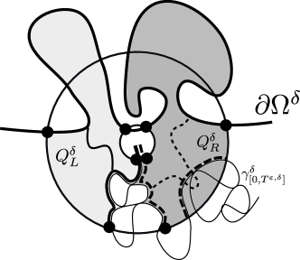
Figure 5.1. The moment $T^{\varepsilon,\delta}$ the curve $\gamma_{t}^{\delta}$ first comes close to the boundary of $\Omega^{\delta}$ away from the arc $(b^{(2n,\delta)},b^{(1,\delta)}).$ The quads $Q_{L}^{\delta}$ and $Q_{R}^{\delta}$ are in light gray and dark gray respectively. Their crossing, respectively, dual crossing, as shown in the picture, forces the event $E^{\varepsilon,\delta}.$

Indeed, consider the annulus $A_{\varepsilon}:=\{2\varepsilon^{2}\leq|z-\gamma_{T^{\varepsilon,\delta}}^{\delta}|\leq\varepsilon\}.$ This annulus is crossed by $\partial\Omega^{\delta}$ as well as by the interface $\gamma_{[0,T^{\varepsilon,\delta}]}^{\delta},$ which means that it is also crossed by the wired $\partial_{\mathrm{wired}}$ and by the free $\partial_{\mathcal{\mathrm{free}}}$ part of $\partial\Omega^{\delta}_{T^{\varepsilon,\delta}}\setminus\partial\Omega^{\delta}$, the left-hand side and the right-hand side of $\gamma_{[0,T^{\varepsilon,\delta}]}^{\delta}$ respectively. We now consider the quads $Q_{R,L}^{\varepsilon,\delta}$, formed by a crossing of $A_{\varepsilon}$ by $\partial_{\mathcal{\mathrm{free}}}$ (respectively, $\partial_{\mathrm{wired}}$) , two arcs of the circles $|z-\gamma_{T^{\varepsilon,\delta}}^{\delta}|=\varepsilon^{2}$ and $|z-\gamma_{T^{\varepsilon,\delta}}^{\delta}|=2\varepsilon^{3}$ up until their first intersection with $\partial\Omega^{\delta}$, and a part of $\partial\Omega^{\delta}$ between these two intersection points, see Figure 5.1. Both quads have large modulus and thus, by RSW, if one puts wired (respectively, free) boundary conditions on their boundaries, with probability $q(\varepsilon)\to 1$ as $\varepsilon\to 0$, they are crossed by a dual cluster (respectively, by a cluster) separating the arcs of the circles. Conditionally on $\gamma_{[0,T^{\varepsilon,\delta}]}^{\delta}$, such crossings are even more likely by monotonicity, since any part of $\partial\Omega^{\delta}_{T^{\varepsilon,\delta}}$ that intersects the interior of the $Q_{R,L}^{\varepsilon,\delta}$ is free (respectively, wired). The coexistence of such crossings implies that $\gamma_{[T_{1}^{\varepsilon,\delta},T_{2}^{\varepsilon,\delta}]}^{\delta}$ hits $\partial\Omega^{\delta}$, which therefore happens with probability at least $2q(\varepsilon)-q(\varepsilon)^{2}.$

For the diameter bound, consider the annulus $A^{\prime}_{\varepsilon}:=\{\varepsilon\leq|z-\gamma_{T^{\varepsilon,\delta}}^{\delta}|\leq\sqrt{\varepsilon}/2\}.$ If the part of $\partial\Omega^{\delta}$ separated from $b^{(1,\delta)}$ by $\omega^{\varepsilon,\delta}$ does not cross that annulus, then neither does $\gamma_{[T_{1}^{\varepsilon,\delta},T_{2}^{\varepsilon,\delta}]}^{\delta}$ and we are done. Otherwise, consider the quad formed by arcs of the inner and outer boundary of $A^{\prime}_{\varepsilon}$ and the first outward and last inward crossing of it by $\partial\Omega^{\delta}.$ By RSW and monotonicity, with probability at least $q^{\prime}(\varepsilon)\to 1$ as $\varepsilon\to 0$, this quad is crossed by an open or by a dual-open path, which prevents $\gamma_{[T_{1}^{\varepsilon,\delta},T_{2}^{\varepsilon,\delta}]}^{\delta}$ from crossing $A^{\prime}_{\varepsilon},$ and thus from having diameter $\geq\sqrt{\varepsilon}.$ All in all, we can take $p(\varepsilon):=q^{\prime}(\varepsilon)+2q(\varepsilon)-q(\varepsilon)^{2}-1.$

With probability going to $1$ as $\varepsilon\to 0$, $\gamma_{[0,\tau]}$ stays at distance at least $3\varepsilon$ from $[b^{(2)},b^{(J)}]\cup[b^{(J+1)},b^{(2n)}].$ On this event, for $\delta$ small enough, $\gamma_{[0,T^{\varepsilon,\delta}]}^{\delta}$ stays at distance at least $2\varepsilon$ from $[b^{(2,\delta)},b^{(J,\delta)}]\cup[b^{(J+1,\delta)},b^{(2n,\delta)}]$, hence $G^{\delta,\varepsilon}$ holds, and $E^{\varepsilon,\delta}$ implies $J^{\delta}=J.$ Therefore, $J^{\delta}\to J$ in probability, and thus almost surely along a subsequence.

Any point $w$ of $\partial\Omega_{L}$ is either a point of $\partial\Omega$, or a point of $\gamma$; in either case there is a sequence of points $w^{\delta}\in\partial\Omega^{\delta}\cup\gamma^{\delta}$ that approximates $w.$ We can find sequences $\varepsilon_{k}$ and $\delta_{k}<\varepsilon_{k}^{2}/10$ such that $\mathsf{\mathbb{P}}(G^{\varepsilon_{k},\delta_{k}})\geq 1-2^{-k}$ and $p(\varepsilon_{k})\geq 1-2^{-k}$; then, Borel–Cantelli and the above argument ensures that almost surely, all but finitely many of $E^{\varepsilon_{k},\delta_{k}}$ happen. But if $w\in\Omega_{L}$, $\mathrm{dist}(w,\partial\Omega_{L})\geq 2\varepsilon$ and $B_{\varepsilon}(w)\nsubseteq\Omega_{L}^{\delta_{k}},$ then, for $k$ large enough, this means that $E^{\varepsilon_{k},\delta_{k}}$ has failed. Therefore, almost surely, for all $w\subset\Omega_{L}$ with rational coordinates, $B_{\mathrm{dist}(w;\partial\Omega_{L})/2}(w)\subset\Omega_{L}^{\delta_{k}}$ for $k$ large enough. This implies $\Omega_{L}^{\delta_{k}}\stackrel{{\scriptstyle\text{Cara}}}{{\longrightarrow}}\Omega_{L};$ same argument applies to $\Omega_{R}^{\delta_{k}}.$ On $E^{\varepsilon_{k},\delta_{k}},$the cross-cut $\omega^{\varepsilon_{k},\delta_{k}}$ actually separates the newly created marked point in $\Omega^{\delta}_{L}$ (if $J$ is even) or $\Omega^{\delta}_{R}$ (if $J$ is odd) from the other marked points, and converges to $\gamma_{\tau}$, which shows $\mathcal{\beta}_{L,R}^{\delta}\to\mathcal{\beta}_{L,R}.$ For the regularity claim, which we also need to check only for the new marked point, we can take $U^{\varepsilon,\delta_{k}}$ to be the part of $\Omega^{\delta}_{L}$ or $\Omega^{\delta}_{R}$ separated by the cross-cut $\omega^{\varepsilon,\delta_{k}}$ from other marked points. The above argument shows that (4.1) holds with $\varepsilon^{\prime}=\max(\sqrt{\varepsilon},q^{\prime}(\varepsilon)).$ ∎

Lemma 5.4 allows for the following inductive definition:

Definition 5.7.

The (global) multiple SLE_16/3 in $\Omega$ is a random collection of curves $\gamma^{(1)},\gamma^{(3)}\dots,\gamma^{(2n-1)}$ connecting $b^{(1)},\dots,b^{(2n-1)}\in\partial\Omega$ to $b^{(2\sigma(1))},\dots,b^{(2\sigma(n))}\in\partial\Omega$ respectively, for some random permutation $\sigma$ of $\{1,\dots,n\}$, defined by the following properties:

• the marginal law of of the curve $\gamma_{[0,\tau]}^{(1)}$ started from $b^{(1)}$ is given by the chordal Loewner evolution with the driving process (5.3).

• conditionally on $\gamma_{[0,\tau]}^{(1)}$, the law of ($\gamma^{(1)},\gamma^{(3)}\dots,\gamma^{(2n-1)}$) is given by independent multiple SLE_16/3 processes in $\Omega_{L,R}$ in which the curve starting from $\gamma_{\tau}$ is concatenated with $\gamma_{[0,\tau]}^{(1)}$.

• the base case $n=1$ is given by the chordal SLE${}_{16/3}.$

Proof of Theorem 1.1 and Corollary 1.3.

Lemma 5.2 and Lemma 5.6 ensure that the marginal distribution of $\gamma_{[0,\tau^{\delta}]}^{(1,\delta)}$ converges to that of $\gamma_{[0,\tau]}^{(1)}$. The full interface $\gamma_{[0,N]}^{(1,\delta)}$ consist of $\gamma_{[0,\tau^{\delta}]}^{(1,\delta)}$, the part from $\tau^{\delta}$ until $\gamma_{t}^{(1,\delta)}$ re-enters $\Omega^{\delta}_{L}$ (if $J$ is odd) or $\Omega^{\delta}_{R}$ (if J is even), and then the part of the interface in $\Omega^{\delta}_{L}$ or $\Omega^{\delta}_{R}$. The proof of Lemma 5.6 ensures that the diameter of the middle part goes to zero in probability. Thus, the domain Markov property, Lemma 5.6 and the induction hypothesis imply that the conditional distribution of $(\gamma^{(1,\delta)}$,$\dots$,$\gamma^{(2n-1,\delta)})$ given $\gamma_{[0,\tau^{\delta}]}^{(1,\delta)}$ converges to the conditional distribution of $(\gamma^{(1)}$,$\dots$,$\gamma^{(2n-1)})$ given $\gamma_{[0,\tau]}^{(1)}$, at least along a subsequence $\delta_{k}.$ Hence the full law of $(\gamma^{(1,\delta)},\dots,\gamma^{(2n-1,\delta)})$ converges to that of $(\gamma^{(1)},\gamma^{(3)}\dots,\gamma^{(2n-1)})$ along $\delta_{k}$. Since such a subsequence can be extracted from any sequence of $\delta\to 0$, no extraction is in fact needed. The random variable $\mathbb{I}_{\pi^{\delta}=\pi}$ is a continuous function of the collection if interfaces and the latter has a conformally invariant scaling limit, therefore, Corollary 1.3 also follows. ∎

References

- [1] Michel Bauer, Denis Bernard, and Kalle Kytölä. Multiple schramm–loewner evolutions and statistical mechanics martingales. Journal of statistical physics, 120(5-6):1125–1163, 2005.
- [2] Vincent Beffara and Hugo Duminil-Copin. The self-dual point of the two-dimensional random-cluster model is critical for . Probability Theory and Related Fields, 153(3-4):511–542, 2012.
- [3] Vincent Beffara, Eveliina Peltola, and Hao Wu. On the uniqueness of global multiple sles. arXiv preprint arXiv:1801.07699, 2018.
- [4] A. A. Belavin, A. M. Polyakov, and A. B. Zamolodchikov. Infinite conformal symmetry in two-dimensional quantum field theory. Nuclear Phys. B, 241(2):333–380, 1984.
- [5] Theodore W. Burkhardt and Ihnsouk Guim. Bulk, surface, and interface properties of the Ising model and conformal invariance. Phys. Rev. B (3), 36(4):2080–2083, 1987.
- [6] Dmitry Chelkak. Planar ising model at criticality: state-of-the-art and perspectives. arXiv preprint arXiv:1712.04192, 2017.
- [7] Dmitry Chelkak. S-embeddings: conformal invariance of the critical ising model beyond z-invariance and isoradial graphs. in preparation, 2020.
- [8] Dmitry Chelkak, David Cimasoni, and Adrien Kassel. Revisiting the combinatorics of the 2D Ising model. arXiv:1507.08242, 2015.
- [9] Dmitry Chelkak, Hugo Duminil-Copin, Clément Hongler, et al. Crossing probabilities in topological rectangles for the critical planar fk-ising model. Electronic Journal of Probability, 21, 2016.
- [10] Dmitry Chelkak, Hugo Duminil-Copin, Clément Hongler, Antti Kemppainen, and Stanislav Smirnov. Convergence of Ising interfaces to Schramm’s SLE curves. C. R. Math. Acad. Sci. Paris, 352(2):157–161, 2014.
- [11] Dmitry Chelkak, Clément Hongler, and Konstantin Izyurov. In preparation.
- [12] Dmitry Chelkak, Clément Hongler, and Konstantin Izyurov. Conformal invariance of spin correlations in the planar Ising model. Ann. of Math. (2), 181(3):1087–1138, 2015.
- [13] Dmitry Chelkak, Benoit Laslier, and Marianna Russkikh. Dimer model and holomorphic functions on t-embeddings of planar graphs. arXiv preprint arXiv:2001.11871, 2020.
- [14] Dmitry Chelkak and Stanislav Smirnov. Universality in the 2D Ising model and conformal invariance of fermionic observables. Invent. Math., 189(3):515–580, 2012.
- [15] Julien Dubédat. Commutation relations for Schramm-Loewner evolutions. Comm. Pure Appl. Math., 60(12):1792–1847, 2007.
- [16] Julien Dubédat. SLE and the free field: partition functions and couplings. J. Amer. Math. Soc., 22(4):995–1054, 2009.
- [17] Hugo Duminil-Copin, Clément Hongler, and Pierre Nolin. Connection probabilities and rsw-type bounds for the two-dimensional fk ising model. Communications on pure and applied mathematics, 64(9):1165–1198, 2011.
- [18] Robert G Edwards and Alan D Sokal. Generalization of the fortuin-kasteleyn-swendsen-wang representation and monte carlo algorithm. Physical review D, 38(6):2009, 1988.
- [19] Steven M. Flores and Peter Kleban. A solution space for a system of null-state partial differential equations: Part 1. Comm. Math. Phys., 333(1):389–434, 2015.
- [20] Steven M. Flores and Peter Kleban. A solution space for a system of null-state partial differential equations: Part 2. Comm. Math. Phys., 333(1):435–481, 2015.
- [21] Steven M. Flores and Peter Kleban. A solution space for a system of null-state partial differential equations: Part 3. Comm. Math. Phys., 333(2):597–667, 2015.
- [22] Steven M. Flores and Peter Kleban. A solution space for a system of null-state partial differential equations: Part 4. Comm. Math. Phys., 333(2):669–715, 2015.
- [23] Sergey Fomin. Loop-erased walks and total positivity. Trans. Amer. Math. Soc., 353(9):3563–3583, 2001.
- [24] Cornelius Marius Fortuin and Piet W Kasteleyn. On the random-cluster model: I. introduction and relation to other models. Physica, 57(4):536–564, 1972.
- [25] K. Graham. On multiple Schramm-Loewner evolutions. J. Stat. Mech. Theory Exp., (3):P03008, 21, 2007.
- [26] Geoffrey Grimmett. The random-cluster model. In Probability on discrete structures, pages 73–123. Springer, 2004.
- [27] Christian Hagendorf, Denis Bernard, and Michel Bauer. The gaussian free field and sle 4 on doubly connected domains. Journal of Statistical Physics, 140(1):1–26, 2010.
- [28] Clément Hongler and Kalle Kytölä. Ising interfaces and free boundary conditions. Journal of the American Mathematical Society, 26(4):1107–1189, 2013.
- [29] Konstantin Izyurov. Smirnov’s observable for free boundary conditions, interfaces and crossing probabilities. Comm. Math. Phys., 337(1):225–252, 2015.
- [30] Konstantin Izyurov. Critical Ising interfaces in multiply-connected domains. Probab. Theory Related Fields, 167(1-2):379–415, 2017.
- [31] Konstantin Izyurov and Kalle Kytölä. Hadamard’s formula and couplings of SLEs with free field. Probab. Theory Related Fields, 155(1-2):35–69, 2013.
- [32] Leo P Kadanoff and Horacio Ceva. Determination of an operator algebra for the two-dimensional ising model. Physical Review B, 3(11):3918, 1971.
- [33] Alex Karrila. Limits of conformal images and conformal images of limits for planar random curves. arXiv preprint arXiv:1810.05608, 2018.
- [34] Alex Karrila. Multiple sle type scaling limits: From local to global. arXiv preprint arXiv:1903.10354, 2019.
- [35] Alex Karrila. Ust branches, martingales, and multiple sle (2). arXiv preprint arXiv:2002.07103, 2020.
- [36] Alex Karrila, Kalle Kytölä, and Eveliina Peltola. Boundary correlations in planar lerw and ust. Communications in Mathematical Physics, pages 1–81, 2019.
- [37] Alex Karrila, Kalle Kytölä, and Eveliina Peltola. Conformal blocks, -combinatorics, and quantum group symmetry. Ann. Inst. Henri Poincaré D, 6(3):449–487, 2019.
- [38] Antti Kemppainen and Stanislav Smirnov. Conformal invariance in random cluster models. ii. full scaling limit as a branching sle. arXiv preprint arXiv:1609.08527, 2016.
- [39] Antti Kemppainen and Stanislav Smirnov. Random curves, scaling limits and Loewner evolutions. Ann. Probab., 45(2):698–779, 2017.
- [40] Antti Kemppainen and Stanislav Smirnov. Configurations of FK Ising interfaces and hypergeometric SLE. Math. Res. Lett., 25(3):875–889, 2018.
- [41] Antti Kemppainen and Stanislav Smirnov. Conformal invariance of boundary touching loops of FK Ising model. Comm. Math. Phys., 369(1):49–98, 2019.
- [42] Antti Kemppainen and Petri Tuisku. in preparation. 2020.
- [43] Michael J. Kozdron and Gregory F. Lawler. Estimates of random walk exit probabilities and application to loop-erased random walk. Electron. J. Probab., 10:1442–1467, 2005.
- [44] Kalle Kytölä and Eveliina Peltola. Pure partition functions of multiple SLEs. Comm. Math. Phys., 346(1):237–292, 2016.
- [45] Kalle Kytölä and Eveliina Peltola. Conformally covariant boundary correlation functions with a quantum group. J. Eur. Math. Soc. (JEMS), 22(1):55–118, 2020.
- [46] Gregory F. Lawler, Oded Schramm, and Wendelin Werner. Conformal invariance of planar loop-erased random walks and uniform spanning trees. Ann. Probab., 32(1B):939–995, 2004.
- [47] Eveliina Peltola and Hao Wu. Crossing probabilities of multiple ising interfaces. arXiv preprint arXiv:1808.09438, 2018.
- [48] Eveliina Peltola and Hao Wu. Global and local multiple SLEs for and connection probabilities for level lines of GFF. Comm. Math. Phys., 366(2):469–536, 2019.
- [49] Oded Schramm. Scaling limits of loop-erased random walks and uniform spanning trees. Israel J. Math., 118:221–288, 2000.
- [50] Oded Schramm and Scott Sheffield. Harmonic explorer and its convergence to . Ann. Probab., 33(6):2127–2148, 2005.
- [51] Oded Schramm and Scott Sheffield. A contour line of the continuum Gaussian free field. Probab. Theory Related Fields, 157(1-2):47–80, 2013.
- [52] Jacob J. H. Simmons, Peter Kleban, Steven M. Flores, and Robert M. Ziff. Cluster densities at 2D critical points in rectangular geometries. J. Phys. A, 44(38):385002, 34, 2011.
- [53] Stanislav Smirnov. Towards conformal invariance of 2D lattice models. In International Congress of Mathematicians. Vol. II, pages 1421–1451. Eur. Math. Soc., Zürich, 2006.
- [54] Stanislav Smirnov. Conformal invariance in random cluster models. I. Holomorphic fermions in the Ising model. Ann. of Math. (2), 172(2):1435–1467, 2010.
- [55] Wendelin Werner. Lectures on two-dimensional critical percolation. arXiv preprint arXiv:0710.0856, 2007.
- [56] Dapeng Zhan. Duality of chordal sle. Inventiones mathematicae, 174(2):309, 2008.
- [57] Dapeng Zhan. The scaling limits of planar lerw in finitely connected domains. The Annals of Probability, 36(2):467–529, 2008.