Knowledge-Based Prediction of Network Controllability Robustness

Abstract

Network controllability robustness reflects how well a networked system can maintain its controllability against destructive attacks. Its measure is quantified by a sequence of values that record the remaining controllability of the network after a sequence of node-removal or edge-removal attacks. Traditionally, the controllability robustness is determined by attack simulations, which is computationally time consuming or even infeasible. In the present paper, an improved method for predicting the network controllability robustness is developed based on machine learning using a group of convolutional neural networks (CNNs). In this scheme, a number of training data generated by simulations are used to train the group of CNNs for classification and prediction, respectively. Extensive experimental studies are carried out, which demonstrate that 1) the proposed method predicts more precisely than the classical single-CNN predictor; 2) the proposed CNN-based predictor provides a better predictive measure than the traditional spectral measures and network heterogeneity.

I Introduction

Complex networks as an interdisciplinary research field has gained growing popularity since the late 1990s, encompassing network science, systems engineering, applied mathematics, statistical physics, and biological as well as social sciences [1, 2, 3, 4]. Scientific studies are trying to understand the essence and characteristics of complex networks while engineering studies are trying to control them for beneficial applications. In the pursuit of networked systems control, whether or not they can be controlled is a fundamental issue, which leads to the basic concept of network controllability [5, 6, 7, 8, 9, 10, 11, 12, 13, 14, 15].

The concept of controllability refers to the ability of a networked system in changing from any initial state to any desired state under a feasible control input in finite time [15]. In retrospect, it was shown that identifying the minimum number of external control inputs (recalled driver nodes), needed to achieve the structural controllability of a directed network, which requires searching for a maximum matching of the network [5]. Thereafter, in [6], an efficient measure is introduced for assessing the state controllability, based on the rank of the network controllability matrix, for both directed and undirected networks.

It took quite a long time for people to understand the intrinsic relation between topology and controllability of a general, mostly directed network. It was found that clustering and modularity have no prominent impact on the network controllability, but degree correlation has a certain effect [7]. It was revealed [8] that random networks of any topology are controllable by an extremely small number of driver nodes if both of its minimum in- and out-degrees are greater than two. A control centrality was introduced in [16] to measure the importance of nodes regarding their roles against random attacks. The network controllability of some canonical graph models is studied and compared in [17]. For growing networks, the evolution of network controllability is investigated in [18]. Moreover, the controllability of multi-input/multi-output networked systems is studied in [10, 19], with necessary and sufficient conditions derived. Recently, it was realized that some special motifs such as loops and chains are beneficial for enhancing the robustness of network controllability against attacks [20, 21, 22]. A comprehensive survey of the subject is presented in [15].

Regarding the controllability robustness against attacks, which includes random failures and malicious destructions, a large number of studies have been reported [23, 24, 25, 16, 26, 27, 28]. For node- or edge-removal attacks, the main issue is to develop a measure that reflects how well the networks can maintain their controllability after the attacks took place. One measure for the network controllability is quantified by the number of driver nodes needed to recover or retain the network controllability after the occurrence of an attack, while its robustness is quantified by a sequence of values that record the remaining levels of the network controllability after a sequence of attacks [21]. To optimize the network robustness, one usually aims to enhance and maintain a highest possible connectedness of the network against attacks [25]. Given a degree-preserving constraint (i.e., the degree of each node remains unchanged through the process of optimization), an edge-rewiring method is proposed in [29], which increases the number of edges between high-degree nodes, so as to generate a new network with a largest $k$-shell component. In [30], the structure of a network is modified by degree-preserving edge-rewiring, where a spectral measure is employed. By optimizing a specified spectral measure of the network through random edge-rewiring, the robustness of the resultant network is enhanced consequently. However, it was noted that the correlation between spectral measures and the robustness is indeed unclear [31]. Nevertheless, given a reliable predictive measure or indicator of the network robustness, optimization algorithms can be applied [32, 33, 34, 35]. In the case that there are more than one predictive measure, multi-objective optimization schemes can be adopted [36, 28]. In [37], it is shown that network robustness against edge- and node-removals can be enhanced simultaneously. A common observation is that heterogeneous networks with onion-like structures are robust against attacks [25, 38, 39, 40]. The evolution of alternative attack and defense is studied in [41], where attack refers to edge-removal and defense means edge-replenishment. The connectedness of the largest-sized cluster is a commonly-used measure for such robustness [25]. It is noted that, although the connectedness robustness has a certain positive correlation with the controllability robustness, they have very different characteristics and measures.

Although the correlation between network topology and network controllability has been investigated, no specific theoretical indicator or performance index was found that can precisely quantify the general network controllability robustness. The nature of the attack methods leads to different measures of the importance of a node (or an edge) in a network. In the literature, degree and betweenness are two commonly-used measures for the importance of nodes and edges, respectively [42].

It was observed that a power-law degree distribution does not necessarily imply a fragile controllability robustness against targeted node-removals; what really contributes to enhance the network controllability robustness is the multi-chain structure [43] and multi-loop structure [20, 21]. Later, it was observed [22] that it is particularly beneficial to the network controllability robustness if the multi-loops are across the entire networks rather than only within local communities. Lately it was empirically observed [44] that to achieve optimal controllability robustness against random node attacks, both in- and out-degree distributions of a directed network should be extremely homogeneous.

On the other hand, in the field of machine learning, deep neural networks have shown powerful capability in performing classification and regression tasks in image processing. Convolutional neural network (CNN) is one kind of effective deep neural network [45]. CNN is able to automatically analyze inner features of a dataset without human interference. But, if the user has some prior knowledge and it can be ensured that such prior knowledge would not mislead machine learning, then CNN will become even much powerful for data analysis and processing. Successful real-world applications of CNNs include text recognition and classification [46, 47, 48], face recognition and detection [49], image segmentation [50], etc.

(a) BA unshuffled

(b) ER unshuffled

(c) QSN unshuffled

(d) SW unshuffled

(e) BA shuffled

(f) ER shuffled

(g) QSN shuffled

(h) SW shuffled

Figure 1: An example of filtering out the generation-based features. The network size $N=200$ with average degree $\langle k\rangle=5.12$.

Traditionally, for large-scale complex networks, their controllability robustness is evaluated by attack simulations, which however are extremely computationally time consuming. The major computational cost includes: 1) to search for the node to attack, e.g., the maximum betweenness node; 2) the calculation of controllability, e.g., Eq. (2). Both have to be calculated iteratively. To improve the efficiency of prediction for controllability robustness, this paper takes a machine learning-based approach to designing a knowledge-based predictor for the controllability robustness (iPCR), which is an improved version of the single CNN-based predictor of the controllability robustness (PCR) developed in [51], taking advantage of available prior knowledge.

One unique feature of this iPCR is that it can be applied to both directed and undirected networks, since there is no essential difference for the CNN to process an image converted from a directed or an undirected network, where the symmetry in the graph-converted image does not affect the learning of the CNN. As such, the proposed iPCR has a much wider application range than other traditional methods.

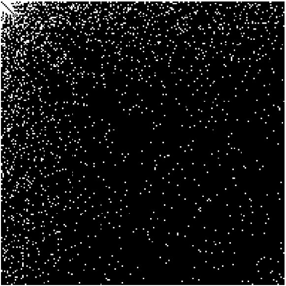
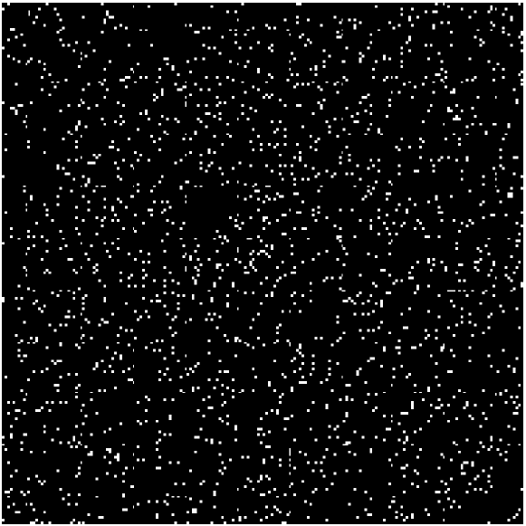
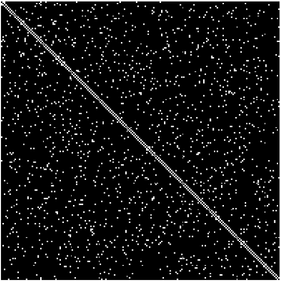
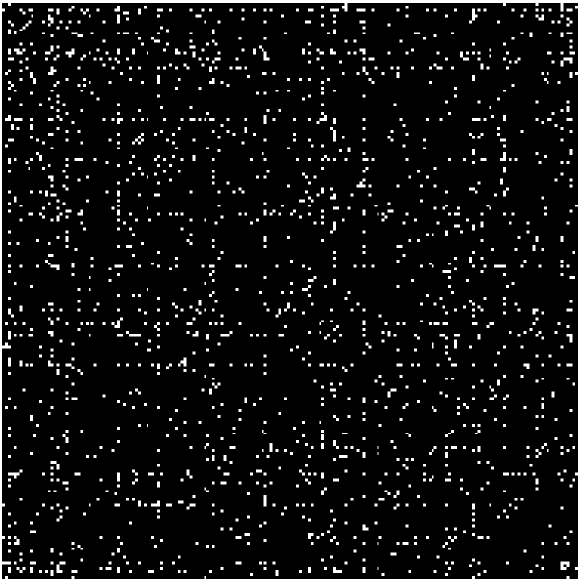
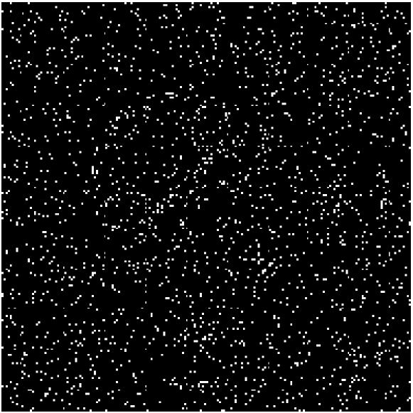
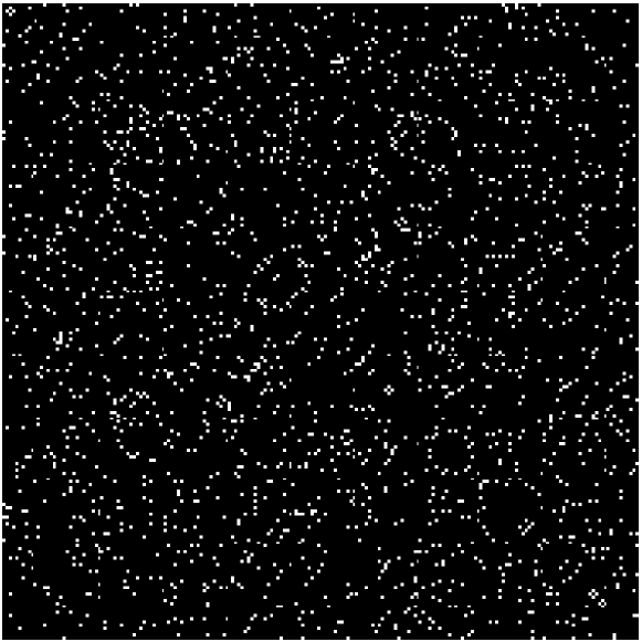
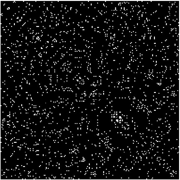
Another improved mechanism in iPCR is that the graph-converted images are updated independently of the generation process. Given an unweighted network, its adjacency matrix can be converted to a black-white image, where a black pixel represents a $0$ element and a white pixel represents a $1$. Given a weighted network with real-valued elements in the adjacency matrix, a gray-scale image is plotted. As shown in Fig. 1, the upper row shows the intrinsic features of the images pertaining to the generation process. These biased features are filtered out by shuffling the rows and columns of the image, as shown in the lower row of the figure. For example, in a Barabási–Albert (BA) scale-free network, the preferential attachment mechanism gives the ‘old’ nodes higher degrees, which are usually allocated near each other therefore have small numbers in the adjacency matrix. As a result, there are always some sparks in the BA-converted image, as shown in Fig. 1 (a). The generation-based features necessarily mitigate the task of a CNN in classification and regression. Therefore, in the iPCR, these special features are filtered out by shuffling the rows and columns of the images, as shown in the lower row of Fig. 1.

To briefly summarize, the proposed design of the iPCR is based on the following observations: 1) there is no clear correlation between the topological features and the controllability robustness of a general network, directed or undirected, 2) the adjacency matrix of a network can be equivalently represented as a gray-scale image, 3) the CNN technique has proved successful in image processing, and 4) prior knowledge at hand could be sufficiently utilized as preprocessing and filtering tools. In the iPCR, a number of training data generated by simulations are used to train the group of CNNs for classification and prediction, respectively.

Extensive experimental studies are carried out, which demonstrate that 1) the proposed method predicts more precisely than the single-CNN predictor; 2) the CNN-based prediction method provides a better predictive measure than the traditional spectral measures and network heterogeneity.

The rest of the paper is organized as follows: Section II reviews the network controllability and its robustness against various destructive attacks. Section III introduces the proposed iPCR. In Section IV, experimental study is performed with analysis. Finally, Section V concludes the investigation.

II Network Controllability and Its Robustness

Consider a linear time-invariant networked system described by $\dot{{\bf x}}=A{\bf x}+B{\bf u}$, where $A$ and $B$ are constant matrices of compatible dimensions, $\bf x$ is the state vector, and $\bf u$ is the control input. The system is state controllable if and only if the controllability matrix $[B\ AB\ A^{2}B\ \cdots A^{N-1}B]$ has a full row-rank, where $N$ is the dimension of $A$, also the size of the networked system. If a system is state controllable, then its state vector $\bf x$ can be driven from any initial state to any desired state in the state space by a suitable control input $\bf u$ within finite time. The concept of structural controllability is a slight generalization dealing with two parameterized matrices $A$ and $B$, in which the parameters characterize the structure of the underlying networked system: if there are specific parameter values that can ensure the parametric system be state controllable, then the system is structurally controllable.

The controllability of a network, or networked system, is measured by the density of the controlled nodes, $n_{D}$, defined by

$$n_{D}\equiv\frac{N_{D}}{N},$$ (1)

where $N_{D}$ is the number of driver nodes needed to retain the network controllability, and $N$ is the network size. This measure $n_{D}$ allows networks with different sizes can be compared. In comparison, the smaller the $n_{D}$ value is, the better the network controllability will be.

For a directed network, the number $N_{D}$ can be calculated according to the minimum inputs theorem derived based on maximum matching [5]. A maximum matching is a matching that contains the largest possible number of edges, which cannot be further extended in the network. A node is matched if it is the end of an edge in the matching; otherwise, it is unmatched. When a maximum matching is found, the number $N_{D}$ of driver nodes is determined by the number of unmatched nodes, i.e. $N_{D}=\text{max}\{1,N-|E^{*}|\}$, where $|E^{*}|$ is the number of edges in the maximum matching $E^{*}$.

As for an undirected network, its controllability can be calculated according to the exact controllability theorem derived based on the controllability matrix [6]. Given an undirected network, its number $N_{D}$ of driver nodes is calculated by

$$N_{D}=\text{max}\{1,N-\text{rank}(A)\}.$$ (2)

The measure of controllability robustness is calculated by

$$n_{D}(i)\equiv\frac{N_{D}(i)}{N-i}\,,\ \ i=1,2,\ldots,N-1,$$ (3)

where $N_{D}(i)$ is the number of driver nodes needed to retain the network controllability after a total of $i$ nodes have been removed, and $N$ is the original network size. When these values are plotted, a curve is obtained, called the controllability curve.

To compare the controllability robustness of two networks against the same attack sequence, their controllability curves are plotted against each other for better visualization. Numerically, a controllability curve $c$ is given by an $(N-1)$ vector $n_{D}^{c}=[n_{D}^{c}(1),n_{D}^{c}(2),\cdots,n_{D}^{c}(N-1)]$. Thus, given two controllability curves, $c_{1}$ and $c_{2}$, the difference (error) of the two curves, when the same number of $i$ nodes are removed, is calculated by

$$\sigma(i)=|n_{D}^{c_{1}}(i)-n_{D}^{c_{2}}(i)|\,.$$ (4)

The average error $\bar{\sigma}$ is then calculated by

$$\bar{\sigma}=\frac{1}{N-1}\sum_{i=1}^{N-1}{\sigma(i)}\,.$$ (5)

The vector $\sigma(i)$ is used to measure the error between the predicted controllability curve against the true curve; while the scalar $\bar{\sigma}$ measures the overall error of prediction.

The overall network controllability robustness $R_{c}$ is defined as [52, 27]

$$R_{c}=\frac{1}{N-1}\sum_{i=1}^{N-1}n_{D}(i)\,,$$ (6)

where, as an extension of the robustness measure defined in [25], $n_{D}(i)$ represents the controllability of the network when a total of $i$ nodes have been removed from the network. Given two complex networks under the same attack, the one with a lower $R_{c}$ value is considered having better controllability robustness.

In the following, for convenience in description, sometimes the integer index sequence $i=1,2,\ldots,N-1$ will be replaced by the fractional index sequence $p=\frac{1}{N},\frac{2}{N},\ldots,\frac{N-1}{N}$, thereby equivalently replacing $n_{D}(i)$ ($i=1,2,\ldots,N-1$) with $n_{D}(p)$ ($p=\frac{1}{N},\frac{2}{N},\ldots,\frac{N-1}{N}$).

III Predictor for Network Controllability Robustness

III-A Framework of Predictor

Figure 2: The framework of PCR [51], where a single CNN is used for controllability robustness (CR) prediction. The input is an image converted from the adjacency matrix; the output is the corresponding controllability curve.

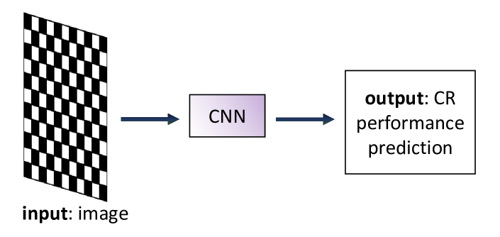
The framework of PCR is shown in Fig. 2, where a single CNN is trained for prediction, referred to as a predictor. This framework straightforwardly performs fairly good predictions, with an overall error less than the standard deviation of the testing samples [51]. However, there are two main issues about this framework. First, many of the PCR predicted controllability curves are vibrating (especially in the initial stage of the attacks), while the real controllability curves are generally smooth. Second, PCR ignores all available prior knowledge, and trains the single CNN using the raw data without any preprocessing. The proposed iPCR addresses the above two issues by employing a multi-CNN structure, with an extra filter.

To address the first issue, in the new framework a data processer called filter is installed after the prediction and before the output. Using available prior knowledge about the dynamics, upper and lower boundaries of the controllability curve can be pre-set. Specifically, during a node-removal attack process, where $i$ ($i=1,2,\ldots,N-1$) nodes are removed, the upper and lower bounds of the controllability curve at position $i$ are pre-set as follows:

$$ub(i)=\frac{\text{min}(N_{D}^{0}+i,N-i)}{N-i}\,,$$ (7)

and

$$lb(i)=\frac{1}{N-i}\,,$$ (8)

where $ub(i)$ and $lb(i)$ represent the upper and lower bounds of $n_{D}(i)$, respectively; $N_{D}^{0}$ means the minimum required number of driver nodes for the original network before being attacked, which can be calculated by Eq. (2).

The following boundary processor is designed:

$$n_{D}(i)=\left\{\begin{array}[]{lr}ub(i),&\text{if }n_{D}(i)>ub(i),\\ lb(i),&\text{if }n_{D}(i)<lb(i).\\ \end{array}\right.$$ (9)

Based on this, a median filter with a mask length $L$ is implemented.

To address the second issue, although human-intervention-free is one of the most attractive properties of deep learning, some available knowledge and common sense may be used if such human knowledge would not mislead the machine learning process. Such prior knowledge of the network data will be preprocessed before prediction. For instance, if the network topology is known beforehand, then the prediction work can be passed to a CNN that is specialized for such a topology, which can have better prediction performance.

Figure 3: The framework of iPCR, where a CNN_c is used for network classification. If the input data can be clearly classified as one specific group, then iPCR uses a specifically trained CNN_$i$, $i=1,2,\ldots,nc$, where $nc$ is the number of clusters; otherwise, if the input data is non-classifiable based on the current knowledge, then iPCR degenerates to PCR using a single CNN_all.

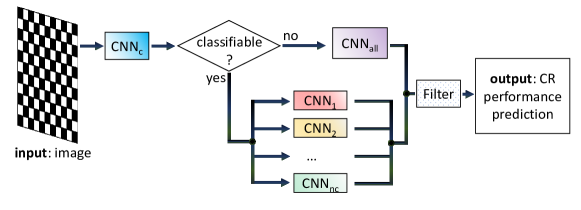
iPCR consists of a group of CNNs, including a classifier CNN_c and several predictors CNN_$i$ ($i=1,2,\ldots,nc$), as shown in Fig. 3. All the predictors have the same CNN structure but are trained by different datasets. Each CNN_$i$ ($i=1,2,\ldots,nc$) is trained by the specific cluster of data, such that it is specialized in predicting a cluster, although probably not suitable for another. CNN_all is trained by all the training data. CNN_c is trained by applying the prior knowledge of the user.

In the experimental study, two types of prior knowledge are tested, namely the network topology (presented in Sec. IV) and the node degree (presented in Supplementary Information (SI) due to space limitation in the paper). Experimental results show that the former provides helpful prior knowledge, while the later is misleading and consequently the prediction results are degenerated. Finally, before outputting the predicted results, iPCR operates a filter that includes a boundary processor (as shown in Eq. (9)) and a median filter.

III-B Convolutional Neural Network

The iPCR framework, which includes a classifier, several predictors and a filter, is now introduced along with its configuration and parameter settings.

Figure 4: [Color online] The architecture of the CNN used for networks classification and controllability robustness prediction, where FM is an abbreviation for feature map, and FC for fully connected. The data sizes $N_{i}=\lceil N/(i+1)\rceil$, $i=1,2,\ldots,7$. The concatenation layer rearranges the matrix into a vector, from FM $7$ to FC $1$, i.e., $L_{0}=N_{7}\times N_{7}\times 512$. $L_{1}\in(L_{0},N-1)$ is a hyperparameter. Set $L_{1}=4096$ in this paper. For prediction, another fully-connected layer FC_p is used as the output layer, yielding an $(N-1)$ vector in the output. For classification, a fully-connected layer FC_c followed by a softmax layer is used. The output is labeled according to the input data.

TABLE I: Parameter settings of the seven groups of convolutional layers.

Group	Layer	Kernel size	Stride	Output channel
Group 1	Conv7-64	7x7	1	64
	Max2	2x2	2	64
Group 2	Conv5-64	5x5	1	64
	Max2	2x2	2	64
Group 3	Conv3-128	3x3	1	128
	Max2	2x2	2	128
Group 4	Conv3-128	3x3	1	128
	Max2	2x2	2	128
Group 5	Conv3-256	3x3	1	256
	Max2	2x2	2	256
Group 6	Conv3-256	3x3	1	256
	Max2	2x2	2	256
Group 7	Conv3-512	3x3	1	512
	Max2	2x2	2	512

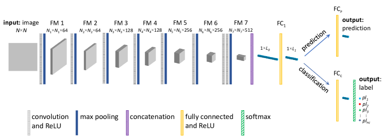
Fig. 4 shows the detailed CNN structure. The detailed parameter settings of the $7$ groups of convolutional layers are given in Table I. Here, the CNN architecture follows the Visual Geometry Group architecture [53]. The number of feature map (FM) groups is set to $7$, since the input size is $1000\times 1000$ in the following experiments. Note that this number should be set to be greater for a larger input dataset. Each FM consists of a convolution layer, a ReLU, and a max pooling layer. A ReLU provides a commonly-used activation function $f(x)=\text{max}(0,x)$ [54]. The output of each hidden layer, i.e., a multiplication of weights, is summed up and then rectified by the ReLU for the next layer. The max pooling layer reduces the dimension of the dataset for the input to the next layer.

For prediction, the output is an $(N-1)$ vector that represents the predicted controllability curve; while for classification, the output is a vector of $nc$ real numbers, $pl_{i}$ ($\sum_{i=1}^{nc}pl_{i}=1$) that represents the probability of the input image belonging to cluster $i$, ($i=1,2,\ldots,nc$). The output layer of the classifier is implemented by adding an extra softmax [55] layer in the end.

A threshold $\eta$ is defined for the classifier such that, only if there exists $pl_{i}\geq\eta$ ($i=1,2,\ldots,nc$), it returns a result indicating that the input image is classifiable (belonging to cluster $i$); otherwise, the input is recognized as non-classifiable. A too-low threshold will decrease the successful rate, while a too-high threshold may result in many non-classifiable cases. In simulations, $\eta$ is set to $0.8$, which yields a successful rate higher than $0.8333$ in classification (see Tables II and III). The results will not be sensitively influenced when $\eta$ is slightly changed.

Note that for different purposes, the internal weights of the CNN will be set differently. Here, for illustration, the structures of predictors and classifiers are plotted together. But a predictor and a classifier do not share any internal weight, and each CNN works independently in iPCR.

The loss function used in the classifier is the cross entropy. Given the predicted and the true probability distribution of an instance, denoted by $pl$ and $tl$ respectively, the cross entropy of this instance is calculated as follows:

$$H=-\sum_{i=1}^{nc}tl(i)\cdot\text{log}[pl(i)]\,.$$ (10)

The loss function used in the predictor is equal to the mean-squared error between the predicted controllability curve $pv$ and the true curve $tc$, which is calculated as follows:

$$\mathcal{L}=\frac{1}{N-1}\sum_{i=1}^{N-1}||pv(i)-tv(i)||\,,$$ (11)

where $||\cdot||$ is the Euclidean norm.

The training process for the classifier and predictor aims at adjusting the weights of CNNs, with the objectives of minimizing the cross entropy in Eq. (10) and the mean-squared error in Eq. (11), respectively.

It is worth mentioning that resizing is commonly used for CNNs to process inputs with different sizes. However, therein the application scenario is different. A row and a column represent a node together with all its connected edges, therefore resizing will change the original topology. Nevertheless, the experimental study presented in Sec. IV-D shows that, if the information loss is very small, the prediction results are still acceptable. There are a few works that deal with different network sizes by using the same CNN, with additional assumptions, for example, [56]. In this paper, CNNs are used to process raw data of complex networks, without any assumption or knowledge on the network structures, and thus the input size can be fixed.

Source codes of this work are available for the public.

IV Experimental Studies

IV-A Experimental Settings

Four typical undirected synthetic networks are adopted for simulation, namely the Barabási–Albert (BA) scale-free network [57], Erdös–Rényi (ER) random-graph network [58], q-snapback network (QSN) [20, 22], and Newman–Watts (NW) small-world network [59].

In the following subsections, the generation methods and parameter settings of the above four networks are introduced, respectively.

Note that, given the network size $N$ and average degree $\langle k\rangle$, there are $M=\lfloor N\cdot\langle k\rangle\rfloor$ edges in total. Standard notation $\lfloor\cdot\rfloor$ and $\lceil\cdot\rceil$ represent the floor and ceiling functions, respectively.

IV-A1 Barabási–Albert (BA) Scale-Free Network

A BA network is generated as follows:

• Start with $n_{0}$ fully-connected nodes (i.e., an $n_{0}$-clique).

• For nodes $i$ ($i=n_{0}+1,\ldots,N$), each of them connects to each of nodes $j$ ($j=1,\ldots i-1$) with a probability of $p_{BA}=\frac{k_{j}}{\sum_{l}k_{l}}$, where $k_{j}$ denotes the degree of node $j$. At each step, there are $e_{BA}$ edges being added preferentially.

Set $n_{0}=\lceil\langle k\rangle\rceil+1$ and $e_{BA}=\frac{M-\binom{n_{0}}{2}}{N-n_{0}}$. To exactly control the number of the generated edges to be $M$, proportionally adding or removing edges can be performed.

IV-A2 Erdös–Rényi (ER) Random-Graph Network

An ER network is generated as follows:

• Start with $N$ isolated nodes.

• Pick up all possible pairs of nodes from the $N$ given nodes, denoted as $i$ and $j$ ($i\neq j$, $i,j=1,2,...,N$), once and once only. Connect each pair of nodes with a probability $p_{ER}\in[0,1]$.

Let $p_{RG}=\frac{\langle k\rangle}{N-1}$. To exactly control the number of the generated edges to be $M$, uniformly-randomly adding or removing edges can be performed.

IV-A3 q-Snapback Network

The q-snapback network (QSN) was originally constructed as a directed network [20] but is converted to be an undirected one here, with only one layer $r_{QSN}$ for simplicity. It is generated as follows:

• Start with a chain of $N$ nodes, where each node $i$ ($i=2,...,N-1$) has two edges connecting to its neighboring nodes $i-1$ and $i+1$.

• For each node $i=r_{QSN}+1,\,r_{QSN}+2,\ldots,N$, it connects backward to the previously-appeared nodes $i-l\times r_{QSN}$ ($l=1,2,\ldots,\lfloor\frac{i}{r_{QSN}}\rfloor$), with the same probability $q\in[0,1]$.

The probability parameter $q$ can be calculated from the given $N$, $M$, and $r_{QSN}$. For $r_{QSN}=1$, $q=\frac{(M-N)\cdot{r_{QSN}}}{\sum_{j=2+r_{QSN}}^{N-2}{j}}=\frac{M-N}{\sum_{j=3}^{N-2}{j}}$. To exactly control the number of the generated edges to be $M$, uniformly-randomly adding or removing edges can be performed.

IV-A4 Newman–Watts (NW) Small-World Networks

An NW network is generated as follows:

• Start with an $N$-node loop having $K$ connected nearest-neighbors on each side.

• Some edges are added without removing any existing edges, until totally $M$ edges have been added.

Set $K=2$ in the following; that is, a node $i$ is connected to its two nearest neighbors on each side, i.e., with nodes $i-1$, $i+1$, $i-2$ and $i+2$.

Since the above generation methods will generate networks with some strong visible features (as illustrated by Fig. 1), the rows and columns of the resulting adjacency matrices are shuffled and random isomorphs are generated, so as to filter out these undesirable features.

The training data are generated by performing attack simulations on the generated networks, such that the controllability curves (see Eq. (3)) can be obtained. These graph-converted images and controllability curves are used for iPCR training. Given an input graph-converted image, the trained iPCR can be used to predict its controllability curve, skipping the time-consuming attack simulation process.

Next, the prediction performances of PCR and iPCR are compared on 1) unweighted networks against random node-removal attacks (see Sec. IV-B), 2) weighted networks against targeted node-removal attacks (see Sec. IV-C); 3) real-world networks under random attacks (see Sec. IV-D). In these three experimental studies, PCR and iPCR aim to predict precise controllability curves. In Sec. IV-E, PCR and iPCR are compared on predicting the ordinal ranks of the network controllability robustness, with respect to $6$ spectral measures and the heterogeneity. Finally, the computational costs are briefly discussed in Sec. IV-F. In all the following comparisons, a filter consisting of a boundary processor and a median filter (with $L=9$) are installed in both PCR and iPCR.

IV-B Unweighted Networks Under Random Attacks

The controllability robustness prediction on unweighted networks with size $N=1000$ and average degree $\langle k\rangle=3$, $4$, and $5$, under random node-removal attacks, is studied.

There are $12$ network configurations in total. For each configuration, $500$ training samples are used. Each sample includes an adjacency matrix (as the input) and its controllability curve obtained from simulation (as the output). CNN_all of iPCR is trained by $12\times 500=6000$ training samples; while each of CNN_1,2,3,4 is trained by $3\times 500=1500$ samples. Each CNN_k ($\text{k}=1,2,3,4$) is specifically trained for one of the four network types, namely BA, ER, QSN, and NW; while CNN_all is trained by the ensemble of all the networks. PCR is trained in the same way as CNN_all of iPCR. Given a random attack, in simulation the result is averaged from $10$ independent runs, so as to balance mitigating and randomness influences, which also reduces the burden of computation.

Another set of $100$ testing samples for each network configuration are generated independently. The classification results of CNN_c are shown in Table II. As illustrated by Fig. 1, shuffling filters out the method-generated features in the resultant images, resulting images indistinguishable by eyes, which makes the classification task becoming tougher. It can be seen from Table II that CNN_c correctly classifies the four types of networks at a successful rate higher than $0.8333$. Since the threshold is set to $\eta=0.8$ in the softmax layer of the classifier, an input is non-classifiable if it generates a result with the probability of success less than $0.8$, and in this case the input will be passed to CNN_all for prediction. As can be seen from Table II, the rate of non-classifiable (NC) data is low, indicating the effectiveness of the classifier which uses prior knowledge.

Note that if an input is incorrectly classified, it will be passed to a wrong predictor that is specialized for a different network type. This will totally mislead the prediction, and therefore is harmful. In iPCR, according to Table II, BA and QSN may be mis-classified as ER at rates $0.0922$ and $0.0165$, respectively; NW may be mis-classified QSN at a rate $0.0042$; ER will not be mis-classified to other networks, but becomes non-classifiable at rate $0.0254$. Overall, the classification error rates are quite low, so iPCR is proved working well.

TABLE II: Confusion matrix of the CNN_c classifier for classifying unweighted networks. NC means the input is non-classifiable; (pre) represents the predicted type and (act) represents the actual type of the network.

	BA (pre)	ER (pre)	QSN (pre)	NW (pre)	NC
BA (act)	0.8333	0.0922	0	0	0.0745
ER (act)	0	0.9746	0	0	0.0254
QSN (act)	0	0.0165	0.9342	0	0.0494
NW (act)	0	0	0.0042	0.9833	0.0126

Figure 5: [Color online] Comparison of PCR and iPCR on unweighted networks under random attacks. $P_{N}$ represents the portion of nodes having been removed from the network; $n_{D}$ is calculated by Eq. (1). Green curves: the true value (tVal) from simulation; red curves: predicted by PCR; black curves: predicted by iPCR. The shaded shadow in the same color represents the range of standard deviation.

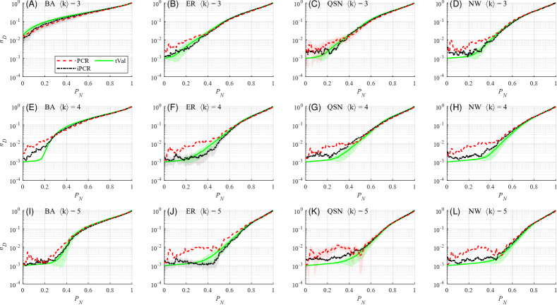
The performance comparison between PCR and iPCR is shown in Fig. 5. In each subplot, in a unique network configuration, the green curve shows the true value (tVal) generated by simulation; the red dashed curve shows the predicted values by PCR; the black dotted curve represents the predicted results of iPCR. The shadow in the same color represents the range of standard deviation. As can be seen from the plots, the black curves are obviously closer to the green curves, better than the red curves, meaning that iPCR predicts the controllability more accurately than PCR, in all $12$ cases. The results confirm that prior knowledge of the network topology is indeed helpful if correctly used. It is notable that the predicted curves are not as oscillatory as those obtained in [51], thanks to the filters used in both PCR and iPCR.

(a) $N$=$1000$, the inset gives a zoom-in for $P_{N}\in[0.9,1]$.

(b) $N$=$600$

(c) $N$=$1200$

(d) weighted, targeted attacks

Figure 6: [Color online] The average errors ($\sigma$) comparison of PCR and iPCR: unweighted networks with (a) $N=1000$, (b) $N=600$, and (c) $N=1200$, under random attacks; (d) weighted networks ($N=1000$) under targeted attacks. The green curve (Std) represents the standard deviation of the testing samples.

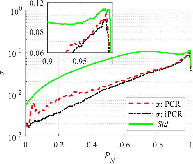
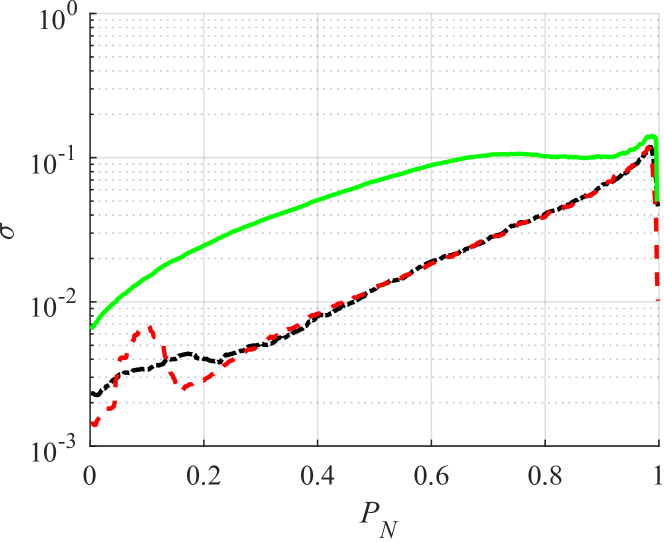
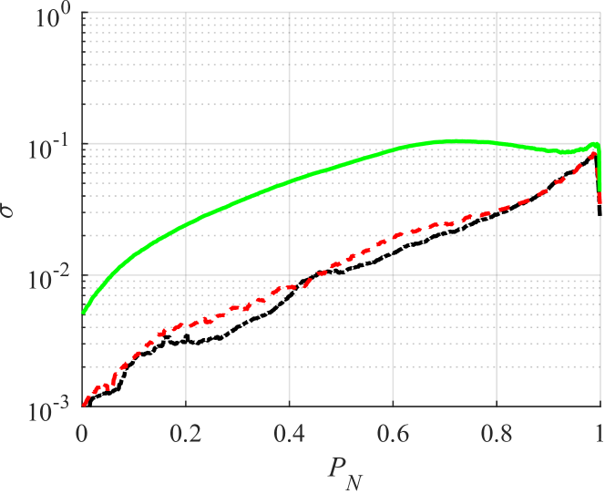
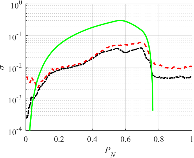
The average error calculated according to Eq. (4) is plotted in Fig. 6 (a), where the black curve shows that iPCR has a lower average error ($\sigma$) than the red dashed curve of PCR, through the entire attacking process. The inset shows a clearer plot of the comparison for $P_{N}\in[0.9,1]$. The average error is taken from all $12$ configurations, namely, a total of $1200$ testing samples. It is noticeable that both PCR and iPCR gain average errors with standard deviations much lower than that of the testing set (i.e., the $1200$ testing samples), throughout the entire attack process.

To verify the scaling property, given the same conditions except for the network size, the prediction performances of iPCR and PCR are compared. Figs. 6 (b) and (c) show the average errors ($\sigma$) comparisons when $N=600$ and $1200$, respectively. The detailed predicted controllability curves are shown in SI.

IV-C Weighted Networks Under Targeted Attacks

The controllability robustness prediction on weighted networks with size $N=1000$ and average degree $\langle k\rangle\in[3,5]$, under targeted node-removal attacks, is studied.

For each network instance, its average degree $\langle k\rangle$ is a real random number generated from the range of $[3,5]$; its edge weights are uniformly-randomly assigned from the range of $(0,1)$. Again, PCR contains a single CNN, while iPCR uses a CNN_all with four specialized CNN_1,2,3,4 for the four types of networks respectively, if classifiable. The targeted attack performs node-removals according to the degrees of nodes, from high to low sequentially.

TABLE III: Confusion matrix of the CNN_c classifier on classifying weighted networks. NC means the input is non-classifiable; (pre) represents the predicted type and (act) represents the actual type of the network; initial ‘w’ is for ‘weighted’.

	wBA (pre)	wER (pre)	wQSN (pre)	wNW (pre)	UC
wBA (act)	0.9913	0	0	0	0.0087
wER (act)	0	0.9549	0.0150	0	0.0301
wQSN (act)	0	0	0.9915	0	0.0085
wNW (act)	0	0	0.0074	0.9815	0.0111

The confusion matrix shown in Table III suggests that the precision of the CNN_c classifier is high. Slightly different from Table II, here the CNN_c can either correctly classify the weighted BA and QSN respectively, or return a result of non-classifiable, without any mis-classification. The weighted ER and NW have very low probabilities to be classified as weighted QSN. Shuffling is also performed on these weighted networks. The overall precision on classifying weighted networks is slightly higher than that on unweighted networks.

In the experiments reported in Sec. IV-B, the average degree $\langle k\rangle$ is set to integers $3,4,5$, respectively. Each column in Fig. 5 shows the same type of networks, with increasing $\langle k\rangle$ from $3$ to $5$. Although PCR and iPCR are trained without any information about the average degrees, both PCR and iPCR return different predictions, when the input is of the same network type with different average degrees. However, this does not imply that average degree is a good feature or useful prior knowledge. In contrast, the average degree is known to be not suitable for preprocessing when used as prior knowledge. An example is given in the SI, where three network clusters are defined, namely ‘$\langle k\rangle=3$’, ‘$\langle k\rangle=4$’, and ‘$\langle k\rangle=5$’. The prediction results is distorted due to the low precision of classification. This demonstrates that the prior knowledge used should be correct and appropriate, as common sense, otherwise misleading could happen.

Figure 7: [Color online] Comparison of PCR and iPCR on weighted networks under targeted attacks. $P_{N}$ represents the portion of nodes having been removed from the network; $n_{D}$ is calculated by Eq. (1). Green curves: the true value (tVal) from simulation; red curves: predicted by PCR; black curves: predicted by iPCR. The shaded shadow in the same color represents the range of standard deviation.

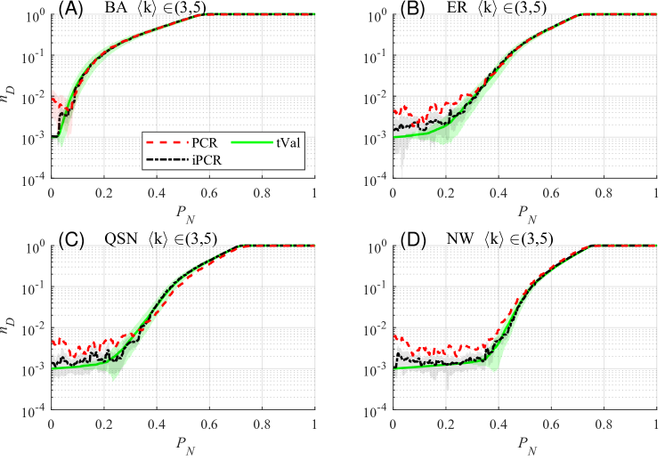
Fig. 7 shows the prediction results of PCR and iPCR on weighted networks under targeted attacks. Again, it is clear that, in each subplot, the black dotted curve is closer to the green curve than the red dashed curve. The higher precision of iPCR in prediction is partially due to the high classification rate presented in Table III. Another reason is that an specialized CNN predictor is always better than a mixed one, as is intuitively so.

Fig. 6 (d) shows that the average prediction error of iPCR (black curve) is lower than that of PCR (red dashed curve), throughout the entire attack process. Note that both PCR and iPCR gain average errors with standard deviations much lower than that of the testing samples through a long period. Differing from random attacks, in a targeted attack, when the portion of removed nodes is somewhat greater than $0.7$, the network requires $n_{D}\approx 1$ to gain a full controllability. Although PCR and iPCR gain lower predictive errors during this stage (when $P_{N}$ is somewhat greater than $0.7$), the standard deviation of the testing sample actually becomes nearly zero.

IV-D Real-world Networks Under Random Attacks

The PCR and iPCR trained in Sec. IV-B are used for predicting the controllability robustness of $6$ real-world networks with $N\approx 1000$. Basic information of these networks is given in Table IV; the network data are from Network Repository .

TABLE IV: Basic information of the real-world networks.

abbr. name	file name	brief description	$N$	$M$
DDG	DD-g79	protein	1022	2889
DEL	delaunay-n10	DIMACS10 problem	1024	3056
DW5	dwt-1005		1005	3808
DW7	dwt-1007	symmetric connection from Washington	1007	3784
LSH	lshp1009	Alan George’s L-shape problem	1009	2928
ORS	orsirr-1	oil reservoir simulation	1030	2914

(a) Prediction Results

(b) Prediction Errors

Figure 8: [Color online] Performance comparison of PCR and iPCR on real-world networks under random attacks: (a) prediction results; (b) prediction errors.

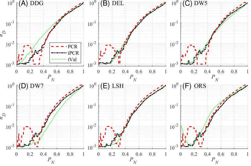
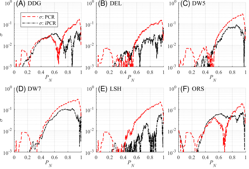
Since the sizes of the real-world networks are slightly larger than $1000$ (see Table IV), resizing is performed on the graph-converted images, i.e., a pair of row and column is randomly picked and removed until it reaches $N=1000$. For each network, the random resizing is repeated for $20$ times, and the prediction results and errors are then averaged. As can be seen from Fig. 8 (a), iPCR predicts the controllability curves closer to the true curves than PCR does, especially in the early stage. Fig. 8 (b) shows that iPCR obtains clearly lower prediction errors than PCR for networks DEL, DW5, DW7 and LSH; while for DDG and ORS, PCR obtains lower errors than iPCR only in a limited period at the middle stage. Both PCR and iPCR predict the controllability performances of these real-world networks with low errors.

IV-E Comparison of Prediction Measures

Spectral measures have long been used to quantify the connectedness robustness of complex networks against node- and edge-removal attacks. It has certain positive correlation to controllability, but they cannot be treated equally.

Here, six commonly-used spectral measures, namely spectral radius (SR), spectral gap (SG), natural connectivity (NCo), algebraic connectivity (ACo), effective resistance (ERe), and spanning tree count (STC) are compared in measuring the controllability robustness. Definitions and computational formulas for these measures can be found in, e.g., [30]. Recently, it was also found that heterogeneity (HE) reflects the controllability robustness [22]. In this paper, PCR and iPCR are used to predict the entire controllability curves in Secs. IV-B and IV-C. Noticed that a predicted curve (a vector) can also be converted to a measure (a scalar) through Eq. (6). Thus, in the following, the above $9$ prediction measures will be compared, namely, the $6$ common spectral measures (SR, SG, NCo, ACo, ERe, STC), HE, PCR and iPCR.

The above prediction measures are used to predict the ordinal ranks of a total of $1200$ networks, for four network types with three different average degrees. These ranks are listed in a descending order in terms of controllability robustness, from the best to the worst. Specifically, each prediction measure returns a predicted rank list of the $1200$ networks. Then, the $9$ rank lists returned by the $9$ prediction measures are compared to the true rank list generated by simulation. The rank error information is summarized in Table V, where the rank error $\sigma_{rank}$ is calculated by

$$\sigma_{rank}=|rl_{pm}-rl_{t}|\,,$$ (12)

where $rl_{pm}$ represents the rank list predicted by a prediction measure, and $rl_{t}$ represents the true rank obtained from simulation.

For example, given two predicted rank lists, $rl_{pm1}=[3,5,2,4,1]$ and $rl_{pm2}=[2,1,4,5,3]$, and a true rank list, $rl_{t}=[1,2,3,4,5]$, the rank errors are obtained as $\sigma_{rank1}=[2,3,1,0,4]$, $\sigma_{rank1}=[1,1,1,1,2]$, respectively. The mean, maximum, and minimum of the rank error can be calculated accordingly. The number of ‘$0$’ elements in a rank error list $\sigma_{rank}$ is counted and then included in the ‘correct rank’ column. Finally, the number of networks, which are predicted top $10\%$ and then confirmed top $10\%$ by simulation, in terms of controllability robustness, is counted and included in the ‘top $10\%$’ column. The number in the ‘bottom $10\%$’ column is similarly calculated. The detailed rank values of the $9$ prediction measures are given in SI.

TABLE V: Rank error information for the $9$ predictive measures. Bold number means the best performing prediction measures.

	average rank error	max rank error	min rank error	correct rank	top 10%	bottom 10%
SR	387.52	912	0	3	0	5
SG	370.09	933	1	0	0	7
NCo	394.58	993	0	3	0	5
ACo	496.98	1095	0	1	0	0
ERe	160.64	704	0	2	52	100
STC	547.14	1192	2	0	0	0
HE	187.13	910	0	2	13	91
PCR	112.72	481	0	2	46	104
iPCR	103.73	590	0	6	45	97

It can be seen from Table V that iPCR receives the minimum average rank error $103.73$, followed by PCR. PCR obtains the minimum max rank error, followed by iPCR. Seven out of nine predictive measures receive a min rank error $0$, meaning that these measures predict at least one rank exactly as the true rank. iPCR predicts $6$ ranks correctly. ERe predicts $52$ top $10\%$ networks that are truly top $10\%$ networks, although their exact ranks may be different, which are followed by PCR and iPCR that correctly predict $46$ and $45$ networks respectively. Finally, PCR well predicts $104$ bottom $10\%$ networks, followed by ERe and iPCR. The test dataset contains $1200$ networks, hence there are $120$ networks ranked as top and bottom $10\%$, respectively.

It is thus clear that PCR and iPCR return better prediction measures than the spectral measures and the heterogeneity. More importantly, PCR and iPCR return not only the predictive measures, but also the entire controllability changing process of a network against the node-removal attack; while the spectral measures and heterogeneity return only a single quantitative value for the controllability robustness.

However, it is notable that PCR and iPCR require a substantial amount of training data, while the spectral measures and heterogeneity do not. Nevertheless, as demonstrated in [51], the overhead in training a CNN is quite low which, compared to the exhaustive attack simulation, is negligible.

IV-F Computational Costs

Compared to PCR, iPCR employs an extra CNN for classification, while the rest computation costs of PCR and iPCR are similar. Thus, the computational cost of iPCR is around two times of that of PCR. As discussed in [51], the cost of simulations to measure the controllability robustness is non-trivial. Compared to simulations, PCR accelerates the prediction speed by hundreds of times.

Given a PC with a 64-bit operation system, installed Intel i7-6700 (3.4 GHz) CPU, GeForce GTX 1080 Ti GPU, to collect a controllability curve for an ER network with $N=1000$ and $\langle k\rangle=5$ under random node attack, the elapsed time is about $162$ seconds for simulation, $0.42$ seconds for PCR, and $1.22$ seconds for iPCR. An example of run time comparison (including PCR, iPCR, and attack simulation) is available on web with source codes.

V Conclusions

Network controllability robustness, which reflects how well a networked system can maintain its controllability after destructive attacks, is usually measured via attack simulations. Such an exhaustive simulation approach can return the true value of the controllability robustness, but is computationally costly and very time consuming. The predictor of controllability robustness (PCR) employs a single convolutional neural network (CNN) to successfully and efficiently achieve the prediction. In this paper, an improved multi-CNN and knowledge-based PCR (iPCR) is designed and evaluated, which takes advantage of prior knowledge from the given data. Extensive experimental studies, with thorough comparisons to seven other comparable measures, demonstrate that 1) iPCR predicts more precisely than PCR; 2) iPCR provides a better predictive measure than the traditional spectral measures and network heterogeneity.

References

- [1] A.-L. Barabási, Network Science. Cambridge University Press, 2016.
- [2] M. E. Newman, Networks: An Introduction. Oxford University Press, 2010.
- [3] G. Chen, X. Wang, and X. Li, Fundamentals of Complex Networks: Models, Structures and Dynamics, 2nd ed. John Wiley & Sons, 2014.
- [4] G. Chen and Y. Lou, Naming Game: Models, Simulations and Analysis. Springer, 2019.
- [5] Y.-Y. Liu, J.-J. Slotine, and A.-L. Barabási, “Controllability of complex networks,” Nature, vol. 473, no. 7346, pp. 167–173, 2011.
- [6] Z. Z. Yuan, C. Zhao, Z. R. Di, W.-X. Wang, and Y.-C. Lai, “Exact controllability of complex networks,” Nature Communications, vol. 4, p. 2447, 2013.
- [7] M. Pósfai, Y.-Y. Liu, J.-J. Slotine, and A.-L. Barabási, “Effect of correlations on network controllability,” Scientific Reports, vol. 3, p. 1067, 2013.
- [8] G. Menichetti, L. Dall’Asta, and G. Bianconi, “Network controllability is determined by the density of low in-degree and out-degree nodes,” Physical Review Letters, vol. 113, no. 7, p. 078701, 2014.
- [9] A. E. Motter, “Networkcontrology,” Chaos: An Interdisciplinary Journal of Nonlinear Science, vol. 25, no. 9, p. 097621, 2015.
- [10] L. Wang, X. Wang, G. Chen, and W. K. S. Tang, “Controllability of networked mimo systems,” Automatica, vol. 69, pp. 405–409, 2016.
- [11] Y.-Y. Liu and A.-L. Barabási, “Control principles of complex systems,” Review of Modern Physics, vol. 88, no. 3, p. 035006, 2016.
- [12] L. Wang, X. Wang, and G. Chen, “Controllability of networked higher-dimensional systems with one-dimensional communication channels,” Royal Society Philosophical Transactions A, vol. 375, no. 2088, p. 20160215, 2017.
- [13] L.-Z. Wang, Y.-Z. Chen, W.-X. Wang, and Y.-C. Lai, “Physical controllability of complex networks,” Scientific Reports, vol. 7, p. 40198, 2017.
- [14] Y. Zhang and T. Zhou, “Controllability analysis for a networked dynamic system with autonomous subsystems,” IEEE Transactions on Automatic Control, vol. 62, no. 7, pp. 3408–3415, 2016.
- [15] L. Xiang, F. Chen, W. Ren, and G. Chen, “Advances in network controllability,” IEEE Circuits and Systems Magazine, vol. 19, no. 2, pp. 8–32, 2019.
- [16] Y.-Y. Liu, J.-J. Slotine, and A.-L. Barabási, “Control centrality and hierarchical structure in complex networks,” PLOS ONE, vol. 7, no. 9, p. e44459, 2012.
- [17] E. Wu-Yan, R. F. Betzel, E. Tang, S. Gu, F. Pasqualetti, and D. S. Bassett, “Benchmarking measures of network controllability on canonical graph models,” Journal of Nonlinear Science, pp. 1–39, 2018.
- [18] R. Zhang, X. Wang, M. Cheng, and T. Jia, “The evolution of network controllability in growing networks,” Physica A: Statistical Mechanics and its Applications, vol. 520, pp. 257–266, 2019.
- [19] Y. Hao, Z. Duan, and G. Chen, “Further on the controllability of networked MIMO LTI systems,” International Journal of Robust and Nonlinear Control, vol. 28, no. 5, pp. 1778–1788, 2018.
- [20] Y. Lou, L. Wang, and G. Chen, “Toward stronger robustness of network controllability: A snapback network model,” IEEE Transactions on Circuits and Systems I: Regular Papers, vol. 65, no. 9, pp. 2983–2991, 2018.
- [21] G. Chen, Y. Lou, and L. Wang, “A comparative study on controllability robustness of complex networks,” IEEE Transactions on Circuits and Systems II: Express Briefs, vol. 66, no. 5, pp. 828–832, 2019.
- [22] Y. Lou, L. Wang, and G. Chen, “Enhancing controllability robustness of q-snapback networks through redirecting edges,” Research, vol. 2019, no. 7857534, 2019.
- [23] P. Holme, B. J. Kim, C. N. Yoon, and S. K. Han, “Attack vulnerability of complex networks,” Physical Review E, vol. 65, no. 5, p. 056109, 2002.
- [24] B. Shargel, H. Sayama, I. R. Epstein, and Y. Bar-Yam, “Optimization of robustness and connectivity in complex networks,” Physical Review Letters, vol. 90, no. 6, p. 068701, 2003.
- [25] C. M. Schneider, A. A. Moreira, J. S. Andrade, S. Havlin, and H. J. Herrmann, “Mitigation of malicious attacks on networks,” Proceedings of the National Academy of Sciences, vol. 108, no. 10, pp. 3838–3841, 2011.
- [26] A. Bashan, Y. Berezin, S. Buldyrev, and S. Havlin, “The extreme vulnerability of interdependent spatially embedded networks,” Nature Physics, vol. 9, pp. 667–672, 2013.
- [27] Y.-D. Xiao, S.-Y. Lao, L.-L. Hou, and L. Bai, “Optimization of robustness of network controllability against malicious attacks,” Chinese Physics B, vol. 23, no. 11, p. 118902, 2014.
- [28] S. Wang and J. Liu, “A multi-objective evolutionary algorithm for promoting the emergence of cooperation and controllable robustness on directed networks,” IEEE Transactions on Network Science and Engineering, vol. 5, no. 2, pp. 92–100, 2018.
- [29] L. Bai, Y.-D. Xiao, L.-L. Hou, and S.-Y. Lao, “Smart rewiring: Improving network robustness faster,” Chinese Physics Letters, vol. 32, no. 7, p. 078901, 2015.
- [30] H. Chan and L. Akoglu, “Optimizing network robustness by edge rewiring: A general framework,” Data Mining and Knowledge Discovery, vol. 30, no. 5, pp. 1395–1425, 2016.
- [31] K. Yamashita, Y. Yasuda, R. Nakamura, and H. Ohsaki, “On the predictability of network robustness from spectral measures,” in 2019 IEEE 43rd Annual Computer Software and Applications Conference (COMPSAC), vol. 2. IEEE, 2019, pp. 24–29.
- [32] L. Hou, S. Lao, B. Jiang, and L. Bai, “Enhancing complex network controllability by rewiring links,” in International Conference on Intelligent System Design and Engineering Applications (ISDEA). IEEE, 2013, pp. 709–711.
- [33] J. Xu, J. Wang, H. Zhao, and S. Jia, “Improving controllability of complex networks by rewiring links regularly,” in Chinese Control and Decision Conference (CCDC), 2014, pp. 642–645.
- [34] J. Liu, H. A. Abbass, and K. C. Tan, “Evolving robust networks using evolutionary algorithms,” in Evolutionary Computation and Complex Networks. Springer, 2019, pp. 117–140.
- [35] S. Wang and J. Liu, “Designing comprehensively robust networks against intentional attacks and cascading failures,” Information Sciences, vol. 478, pp. 125–140, 2019.
- [36] R. C. Gunasekara, C. K. Mohan, and K. Mehrotra, “Multi-objective optimization to improve robustness in networks,” in Multi-Objective Optimization. Springer, 2018, pp. 115–139.
- [37] A. Zeng and W. Liu, “Enhancing network robustness against malicious attacks,” Physical Review E, vol. 85, no. 6, p. 066130, 2012.
- [38] Z.-X. Wu and P. Holme, “Onion structure and network robustness,” Physical Review E, vol. 84, no. 2, p. 026106, 2011.
- [39] T. Tanizawa, S. Havlin, and H. E. Stanley, “Robustness of onionlike correlated networks against targeted attacks,” Physical Review E, vol. 85, no. 4, p. 046109, 2012.
- [40] Y. Hayashi and N. Uchiyama, “Onion-like networks are both robust and resilient,” Scientific Reports, vol. 8, 2018.
- [41] L. Ma, J. Liu, and B. Duan, “Evolution of network robustness under continuous topological changes,” Physica A: Statistical Mechanics and its Applications, vol. 451, pp. 623–631, 2016.
- [42] C.-L. Pu, W.-J. Pei, and A. Michaelson, “Robustness analysis of network controllability,” Physica A: Statistical Mechanics and its Applications, vol. 391, no. 18, pp. 4420–4425, 2012.
- [43] X.-Y. Yan, W.-X. Wang, G. Chen, and D.-H. Shi, “Multiplex congruence network of natural numbers,” Scientific Reports, vol. 6, p. 23714, 2016.
- [44] Y. Lou, L. Wang, K.-F. Tsang, and G. Chen, “Towards optimal robustness of network controllability: An empirical necessary condition,” IEEE Transactions on Circuits and Systems I: Regular Papers, vol. 67, no. 9, pp. 3163–3174, 2020.
- [45] J. Schmidhuber, “Deep learning in neural networks: An overview,” Neural Networks, vol. 61, pp. 85–117, 2015.
- [46] T. Wang, D. J. Wu, A. Coates, and A. Y. Ng, “End-to-end text recognition with convolutional neural networks,” in International Conference on Pattern Recognition (ICPR 2012). IEEE, 2012, pp. 3304–3308.
- [47] S. Lai, L. Xu, K. Liu, and J. Zhao, “Recurrent convolutional neural networks for text classification,” in AAAI Conference on Artificial Intelligence, 2015, pp. 2267–2273.
- [48] X. Zhang, J. Zhao, and Y. LeCun, “Character-level convolutional networks for text classification,” in Advances in Neural Information Processing Systems (NIPS 2015), 2015, pp. 649–657.
- [49] H. Li, Z. Lin, X. Shen, J. Brandt, and G. Hua, “A convolutional neural network cascade for face detection,” in IEEE Conference on Computer Vision and Pattern Recognition (CVPR), 2015, pp. 5325–5334.
- [50] O. Ronneberger, P. Fischer, and T. Brox, “U-net: Convolutional networks for biomedical image segmentation,” in International Conference on Medical Image Computing and Computer-Assisted Intervention. Springer, 2015, pp. 234–241.
- [51] Y. Lou, Y. He, L. Wang, and G. Chen, “Predicting network controllability robustness: A convolutional neural network approach,” IEEE Transactions on Cybernetics, 2020, doi:10.1109/TCYB.2020.3013251.
- [52] J. Ruths and D. Ruths, “Robustness of network controllability under edge removal,” in Complex Networks IV. Springer, 2013, pp. 185–193.
- [53] K. Simonyan and A. Zisserman, “Very deep convolutional networks for large-scale image recognition,” arXiv Preprint: 1409.1556, 2014.
- [54] X. Glorot, A. Bordes, and Y. Bengio, “Deep sparse rectifier neural networks,” in International Conference on Artificial Intelligence and Statistics, 2011, pp. 315–323.
- [55] C. M. Bishop, Pattern Recognition and Machine Learning. springer, 2006.
- [56] M. Niepert, M. Ahmed, and K. Kutzkov, “Learning convolutional neural networks for graphs,” in International Conference on Machine Learning (ICML), 2016, pp. 2014–2023.
- [57] A.-L. Barabási and R. Albert, “Emergence of scaling in random networks,” Science, vol. 286, no. 5439, pp. 509–512, 1999.
- [58] P. Erdös and A. Rényi, “On the strength of connectedness of a random graph,” Acta Mathematica Hungarica, vol. 12, no. 1–2, pp. 261–267, 1964.
- [59] M. E. Newman and D. J. Watts, “Renormalization group analysis of the small-world network model,” Physics Letters A, vol. 263, no. 4–6, pp. 341–346, 1999.