The Impact of Realistic Foreground and Instrument Models on 21 cm Epoch of Reionization Experiments

Abstract

Predictions for the ability of 21-cm interferometric experiments to discriminate Epoch of Reionization (EoR) signal models are typically limited by the simplicity of data models, whereby foreground signals and characteristics of the instrument are often simplified or neglected. To move towards more realistic scenarios, we explore the effects of applying more realistic foreground and instrument models to the 21cm signal, and the ability to estimate astrophysical parameters with these additional complexities. We use a highly-optimized version of 21cmFAST, integrated into 21cmMC, to generate lightcones of the brightness temperature fluctuation for Bayesian parameter estimation. We include a statistical point-source foreground model and an instrument model based on the Murchison Widefield Array (MWA) scaled in observation time to have an effective sensitivity similar to the future Square Kilometre Array (SKA). We also extend the current likelihood prescription to account for the presence of beam convolution and foregrounds, the 2-Dimensional Power Spectrum (PS), and the correlation of PS modes. We use frequency bands between 150 and 180 MHz to constrain the ionizing efficiency ($\zeta$), the minimum virial temperature of halos ($T_{\mathrm{vir}}$), the soft X-ray emissivity per unit Star Formation Rate (SFR) ($L_{X}/SFR$ ), and the X-ray energy threshold ($E_{0}$). We find that the inclusion of realistic foregrounds and instrumental components biases the parameter constraints due to unaccounted for cross-power between the EoR signal, foregrounds and thermal noise. This causes estimates of $\zeta$ to be biased by up to $5\sigma$ but the estimates of $T_{vir}$, L_X/SFR and E₀ remain unaffected and are all within $1\sigma$.

1 Introduction

The Cosmic Dawn (CD) and the subsequent Epoch of Reionization (EoR) mark the end of the cosmic dark ages, during which time the baryonic content of the dark, early universe existed in a warm, neutral state. The intergalactic medium (IGM), predominantly comprised of hydrogen, was illuminated by photons from the first ionizing sources, forming regions of reionized hydrogen with temperatures contrasting with the neutral IGM and background CMB (Barkana & Loeb 2001; Furlanetto et al. 2006). The significance of these periods is prevalent in almost all areas of astrophysics, particularly in understanding the transition between the current and early universe as well as the formation of primordial structures in the universe.

A key probe into these epochs is the imprint of the 21 cm spin-flip transition of neutral hydrogen (Hi) that is redshifted into the low-frequency radio regime. Recently, the Experiment to Detect the Global Epoch of Reionization Signature (EDGES) published a measurement of a flattened absorption profile with timing that somewhat coincides with the expected Hi signal from the CD (Bowman et al., 2018), although it needs further verification from independent experiments. Detection of the EoR, however, has not been reported and remains one of the key science goals of most current low-frequency interferometric telescopes (e.g., the Murchison Widefield Array (MWA) ((Tingay et al., 2013; Wayth et al., 2018)), the Hydrogen Epoch of Reionization Experiment (HERA) (DeBoer et al., 2017), and the Low Frequency Array (LOFAR) (Van Haarlem et al., 2013)).

Since direct imaging of the EoR remains beyond the sensitivity capabilities of current experiments, these instruments aim to detect the spatial fluctuations of the averaged power spectrum. In the near future, however, upcoming low-frequency interferometers such as the Square Kilometre Array (SKA) (Dewdney et al., 2009) and the final phase of HERA are expected to have the sensitivity to directly detect the tomographic imprints of the EoR.

Even with experiments focused on the detection of the variance instead of direct imaging of the EoR signal, its detection is still challenging due to astrophysical foregrounds and other contaminants. These include foregrounds from Galactic and extragalactic origins (Jelić et al. 2010; Gleser et al. 2008), ionospheric distortion (Jordan et al., 2017), instrument noise and radio frequency interference (Bentum et al., 2008; Offringa et al., 2015). The foregrounds prove to be the primary contaminant as they are expected to be up to 5 orders of magnitude brighter than the 21 cm signal (Pritchard & Loeb, 2012). Various foreground mitigation and removal methods have been extensively studied (e.g. see Liu & Shaw (2019) for details); however, for foreground removal method such as source peeling, residual power is still left in the power spectrum due to our incomplete knowledge of the extra-galactic foregrounds. This is due to imperfect peeling and fainter sources existing below the peeling threshold (Datta et al., 2010; Trott et al., 2012; Morales et al., 2012; Vedantham et al., 2012).

Exploration of a physical understanding of the EoR is performed through theoretical simulations of the sources and signal to help supplement observations and constrain the signal. In particular, most simulation work has focused on establishing the roles of the first ionising sources and finding the impact of astrophysical parameters on the Hi signal (see eg. Barkana & Loeb 2001; Ricotti & Ostriker 2004; Madau et al. 2004; Knevitt et al. 2014). Although countless parameters may affect the EoR signal whose estimates vary across the literature, some of the most influential EoR parameters (and their generally-accepted estimates) are: the number of ionizing photons per baryon (N${}_{\gamma}\sim$ 4000) (Barkana & Loeb, 2005); the power-law scale of the baryonic gas fraction in stars with source halo mass ($\alpha_{*}\approx$ 0.5) (Behroozi & Silk, 2015; Ocvirk et al., 2016); and the number of times a hydrogen atom recombines (n${}_{rec}\approx$ 1) (Sobacchi & Mesinger, 2014).

The ultimate goal of understanding the EoR from 21 cm observations will require constraining these parameters using theoretical models . It involves quantitatively evaluating the cosmic EoR signal by making use of one of the many existing EoR simulations, usually semi-numerical, to extract information on the astrophysics. Aside from comparing the results of fiducial reionization simulations with experimental data (Choudhury & Ferrara, 2005), other methods used to achieve this goal include using the maximum likelihood ($\chi^{2}$) fitting (Barkana, 2009), and Bayesian analyses via model selection (Binnie & Pritchard, 2019) or Monte Carlo Markov Chain (MCMC) methods (see eg. Harker et al., 2011; Patil et al., 2014; Greig & Mesinger, 2015; Hassan et al., 2017). Alternative methods to on-the-fly MCMC sampling include emulating simulations using the power spectrum (Kern et al., 2017) and using artificial neural networks (Shimabukuro et al., 2017; Schmit & Pritchard, 2017) or convolutional neural network (Gillet et al., 2019).

A particularly powerful existing code that uses the MCMC approach is 21cmMC (Greig & Mesinger, 2015, 2017, 2018). 21cmMC is a parallelized, efficient EoR analysis code that wraps the publicly-available EoR semi-numerical simulator 21cmFAST (Mesinger et al., 2011) into its Bayesian MCMC framework to produce an EoR lightcone per-iteration. It uses the differential brightness temperature field, constructed as a lightcone, to compute the spherically averaged power spectrum that is, in turn, used in the likelihood prescription.

Previous applications of 21cmMC have used 21cmSense to gauge the uncertainties in the 1-Dimensional (1-D) power spectrum arising from the instrumental noise and smooth foregrounds, completely excising spherical $k$-modes dominated by the latter (Pober et al., 2013, 2014). While this approach is a good first-order approximation, it does not account for potential residual foreground contamination in $k$-modes that it uses due to more complicated instrumental systematics. This can cause difficulties in disentangling contamination and signal power, thus possibly leading to a biased estimate of reionization parameters. Moreover, it does not account for the induced chromaticity from the instrument on the 21 cm signal.

This work provides an extension to 21cmMC, in the publicly-available plug-in py21cmmc-fg. Using this framework, we aim to explore the impact of foreground and instrumental components on the ability to constrain the astrophysical parameters of the EoR. We apply a statistical point-source foreground model and an MWA-based instrument model to the 21cmMC lightcone outputs before averaging to a power spectrum. It is these “corrupted” lightcones that we use to estimate observed power spectra within the MCMC framework, thereby investigating more realistic constraints on astrophysical parameters.

The paper is structured as follows. We first setup the mathematical framework, which includes describing the foreground and instrumental effects we employ in our analysis, in §2. In §3, we analyze the observational effects on the EoR lightcones and in §4, we present the MCMC analysis using 21cmMC with our pipeline. We then discuss the results in §5 and conclude in §6.

2 Mathematical Framework

2.1 Interferometric Visibilities

The baseline displacement, u, is defined as $\mathbf{u}=\mathbf{x}/\lambda$, where x is the physical displacement between the baseline tiles and $\lambda$ is the wavelength. We define the sky coordinate as $\mathbf{l}=(l,m)=(\sin\theta\cos\phi,\sin\theta\sin\phi$), where $\theta$ is the zenith angle, and $\phi$ the angle around the zenith pole.

Based on these definitions, the measured correlation of the electric fields between two sensors for an interferometric observation, the visibility $V(\textbf{u},\nu)$ at frequency $\nu$, in the flat-sky approximation is defined as

$$V(\textbf{u},\nu)=\int I(\textbf{l},\nu)B(\textbf{l},\nu)\exp(-2\pi i\textbf{u}\cdot\textbf{l})d\textbf{l}\ \ \ \mathrm{[Jy]},$$ (1)

with $I(\textbf{l},\nu)$ and $B(\textbf{l},\nu)$ being the intensity of each point-source and beam attenuation at sky coordinate l and frequency $\nu$, respectively. Using the flat-sky approximation whereby the effects of curvature are neglected, we assume that the observed interferometric visibility is identical to the Fourier Transform of the product of signal and the beam model. We will address the second-order effects of spatial curvature on the visibility in future work.

2.2 Brightness Temperature and Power Spectrum

The EoR differential brightness temperature, $\delta T_{b}$, can be quantified by (Furlanetto et al., 2006)

$$\delta T_{b}(z)\approx 27x_{HI}(1+\delta_{nl})\left(\frac{H(z)}{\mathrm{d}v/\mathrm{d}r+H(z)}\right)\left(1-\frac{T_{\gamma}}{T_{s}}\right)$$

$$\times\left(\frac{1+z}{10}\frac{0.15}{\Omega_{m}h^{2}}\right)^{\frac{1}{2}}\left(\frac{\Omega_{b}h^{2}}{0.023}\right)\ [{\rm mK}].$$ (2)

Here, $x_{\mathrm{HI}}$ is the neutral fraction, $\delta_{\mathrm{nl}}$ is the evolved Eulerian overdensity, $H$ is the evolving Hubble constant, d$v$/d$r$ is the gradient of the line-of-sight velocity component, $T_{\gamma}$ is the temperature of the CMB, $T_{\mathrm{s}}$ is the spin temperature of Hi, $z$ is the redshift, $\Omega_{m}$ is the dimensionless matter density parameter, $\Omega_{b}$ is the dimensionless baryonic density parameter and $h$ is the normalized Hubble constant.

For interferometric observations, the power spectrum (hereafter PS), is the primary metric used to characterise the EoR signal. It measures the spatial variance of a signal over a spatial volume $V$ and is defined as

$$P(k)\equiv\frac{|\langle\delta T_{b}^{\dagger}(\vec{k})\delta T_{b}(\vec{k})\rangle_{|\vec{k}|=k}|}{V}\ \ \ [{\textrm{mK}}^{2}{\textrm{ Mpc}^{-3}h^{3}}],$$ (3)

where $k$ is the spatial scale in Fourier space. The PS can be computed either directly from the image cube or from the observed interferometric visibilities, whereby the signal is spherically-averaged over the 3-D spatial scales and is normalised by the volume of the observed area of the sky. The dimensionless 1-D PS is given by

$$\Delta^{2}(k)=\frac{k^{3}}{2\pi^{2}}P(k)\ \ \ [{\rm mK}^{2}],$$ (4)

and is routinely used in current experiments.

It is useful, however, to first compute the cylindrically-averaged 2-D PS, $P(k_{\bot},k_{\parallel})$. The angular and line-of-sight modes of the 2-D PS, $k_{\perp}$ and $k_{\parallel}$, are converted from the Fourier dimensions following (Morales & Wyithe, 2010)

$$k_{\perp}=\frac{2\pi|\textbf{u}|}{D_{M}(z)}\ \ \ [{\rm Mpc^{-1}h}],$$ (5)

and

$$k_{\parallel}=\frac{2\pi H_{0}f_{21}E(z)}{c(1+z)^{2}}\eta\ \ \ [{\rm Mpc^{-1}h}].$$ (6)

Here, $z$ is the observation redshift, $D_{M}(z)$ is the transverse comoving distance, $H_{0}$ is the Hubble constant, $f_{21}$ is the rest frequency of the 21 cm hydrogen hyperfine transition and $E(z)$ is defined as

$$E(z)=\sqrt[]{\Omega_{m}(1+z)^{3}+\Omega_{k}(1+z)^{2}+\Omega_{\Lambda}},$$ (7)

where $\Omega_{\Lambda}$, and $\Omega_{k}$ are the dimensionless density parameters for dark energy and the curvature of space (Hogg, 1999). Because the 2-D PS bins the signal into separable perpendicular and line-of-sight modes, it effectively allows for the management of systematic effects arising from the different modes, and hence is commonly used as an initial step to decontaminate the cosmological EoR signal from the foregrounds. Colloquially termed the “wedge”, the broad region of cylindrical $k$-space dominated by the foregrounds can be understood as the signature of smooth-spectrum foregrounds when being sampled by an imperfect instrument (Vedantham et al., 2012; Trott et al., 2012; Parsons et al., 2012; Datta et al., 2010). The key imperfections are the band-limiting attenuation due to the primary beam, and the discrete sampling of an interferometer, where the sampled wavemodes change with frequency (“chromaticity”).

2.3 Components of Observable Signal

In this subsection, we present the mathematical framework of the different components of the observable signal, which is made of the EoR signal and foregrounds as observed by our instrument model.

2.3.1 EoR Lightcones and Parameters

We use a model $\delta T_{b}$ field generated by 21cmFAST wrapped in 21cmMC. 21cmFAST is a semi-numerical EoR modelling tool designed to efficiently simulate the 21-cm Hi signal using approximate methods combining the excursion-set formalism (Bond et al., 1991; Furlanetto et al., 2004) and perturbation theory. The code generates realizations of $\delta_{nl}$, ionization, peculiar velocity, and $T_{s}$ in 3D which are then combined to compute $\delta T_{b}$ during the EoR. The astrophysical parameters involved in the code are customizable, allowing for the exploration of models and parameter space affecting the EoR (Mesinger et al., 2011, 2014).

The key parameters that we are primarily interested in are:

• the ionizing efficiency i.e., the number of ionizing photons escaping into the IGM per baryon ($\zeta$ [dimensionless])

• the minimum virial temperature of halos required to form stars in galaxies ($T_{\mathrm{vir}}$ [K])

• the soft X-ray emissivity per unit Star Formation Rate (SFR) escaping galaxies ($L_{X}/SFR$ [erg s^-1 keV^-1 M${}^{-1}_{\odot}$ yr])

• the X-ray energy threshold for self-absorption by galaxies ($E_{0}$ [keV]).

These four parameters are chosen due to their relatively high influence on the $\delta T_{b}$ field, as they directly affect the parameters governing $T_{b}$ given by Eq. 2.2, particularly $x_{\mathrm{HI}}$. The fiducial values (and ranges) we adopt are based on Greig & Mesinger (2017), Park et al. (2019) and Gillet et al. (2019) and summarised in Table 1. We note that we only use these values in our final analysis in §5. For exploration and validation purposes presented in §3 and 4, we use the default parameters of $\zeta=30$ and log${}_{10}(T_{vir}/\rm K)=4.7$. We also use the same random seed to generate the signal throughout this research.

Parameter	Fiducial Value	Range
$\zeta$	20.0	[10, 250]
log${}_{10}(T_{\rm vir}$)	4.48	[4, 6]
log${}_{10}(L_{X}/$SFR)	40.5	[38, 42]
E0	0.5	[0.1, 1.5]

Table 1: Fiducial astrophysical parameters and their ranges adopted in this work.

We assume a $\Lambda$ Cold Dark Matter ($\Lambda$CDM) universe using the default cosmological parameters values of 21cmFAST ($h$ = 0.68, $\Omega_{b}$=0.048, $\Omega_{m}$= 0.31, $\Omega_{k}$=0, and $\Omega_{\Lambda}$= 0.69), consistent with results from Planck (2016).

The conversion from $T_{b}$ to flux density $S(\nu)$ is given by the beam-modified Rayleigh-Jeans law,

$$S(\nu)=\left(\frac{2k_{B}T_{b}}{A_{\rm eff}}\right)\Omega\times 10^{26}\ \ \ [{\rm Jy}],$$ (8)

where $k_{B}$ is the Boltzmann constant, $A_{\rm eff}$ is the effective area of the tile (units of m²) and $\Omega$ is the angular size of the beam (units sr).

2.3.2 Point-Source Foreground Model

We use a simple point-source foreground model to simulate the effects of extra-galactic foreground sources based on the power-law relation,

$$\frac{dN}{dS}(S,\nu)=\alpha S_{\nu}^{-\beta}\left(\frac{\nu}{\nu_{0}}\right)^{-\gamma\beta}[{\rm Jy}^{-1}{\rm sr}^{-1}].$$ (9)

Here, $dN/dS$ is the source spatial density per unit flux density, $S_{\nu}$ is the flux at a specific frequency $\nu$, $\beta$ is the slope of the source-count function, and $\gamma$ is the mean spectral-index of point sources. We fiducially use $\alpha$ = 4100 Jy^-1 sr^-1, $\beta$ = 1.59, and $\gamma=0.8$ at $\nu_{0}$ = 150 MHz based on an observational result from Intema et al. (2011).

Our adopted statistical foreground model, while an improvement over previous modeling in the context of parameter estimation, is by no means complete. It ignores potential point-source clustering (Murray et al., 2017), ionospheric effects (Jordan et al., 2017; Mevius et al., 2016; Trott et al., 2018), and more subtly, any potential correlations of the foregrounds with their antecedent EoR counterparts. More importantly, we have not included a galactic diffuse foreground model in this work. These effects are expected to be second-order, except for the diffuse emission, which is bright and spatially-structured. These components are left as extensions to this work.

2.3.3 MWA and SKA-based Instrument Model

Our instrument components are based on the MWA (Tingay et al., 2013; Wayth et al., 2018) and the future SKA (Dewdney et al., 2009). The MWA is a low-frequency radio aperture array telescope located at the Murchison Radio Astronomy Observatory (MRO) site in Western Australia. The array consists of 128 connected tiles with an effective area per tile ($A_{\rm eff}$) of 21 m² at 150 MHz. Each tile consists of a 4x4 grid of dual polarization dipoles with a full-width half-maximum field of view of 26^∘ at $\nu_{0}=150$ MHz. It operates in the 80 – 300 MHz frequency range, making it an excellent probe of the redshifted EoR signal. As one of its primary scientific goals, the MWA reionization observing scheme spans two 30 MHz bands, between 137 – 167 MHz and 167 – 197 MHz (Jacobs et al., 2016).

The low-frequency part of the future SKA (SKA-low) will be located at the MRO alongside the MWA (Dewdney et al., 2009; Mellema et al., 2013). It is expected to have a frequency resolution of 1 kHz with a frequency band of 50 to 200 MHz, and a Field-Of-View (FOV) of 2.5^∘ – 10^∘.

The instruments themselves are hugely complicated; e.g., primary beam responses change between antennas, pointing and polarisation, the dipole array structure yields complex, frequency-dependent beam patterns, signal transport over coaxial cable can lead to cable reflections (imprinting frequency structure into the signal chain), and the large FOV introduces wide-field effects. We restrict ourselves to the primary instrumental response, including baseline sampling, FOV, and frequency-dependent primary beams, because these are the leading-order effects, and leave other instrumental effects to future work. We also neglect the fact that the earth is rotating and assume a fixed zenith pointing at the same patch of the sky. Neglecting the rotation of the Earth changes the $uv$ coverage of the visibilities, hence the sample variance is different, and, due to the wide FOV of the MWA, amounts to a reduction of the overall thermal noise by (only) a factor of up to three on long baselines for the same total integration time. While this should be kept in mind, it is tangential to the point of our present work, and will be explored in more detail in future work.

We approximate the beam attenuation, $B(\textbf{l},\nu)$, to be Gaussian-shaped with

$$B(\textbf{l},\nu)=\exp\left(\frac{-|\textbf{l}|^{2}}{\sigma_{\rm beam}^{2}(\nu)}\right),$$ (10)

where

$$\sigma_{\rm beam}(\nu)\simeq\frac{\epsilon c}{\nu D}.$$ (11)

Here, $\epsilon\simeq 0.42$ is the scaling from the more natural Airy disk to a Gaussian width, $c$ is the speed of light and $D$ is the tile diameter (4 m for the MWA). Although the wide field-of-view of the MWA renders the flat sky-approximation (and hence Eq. 1) inaccurate (Thyagarajan et al., 2015a, b), we will still use it as a reasonable first approximation as the curved-sky treatment will be much more important when using a more realistic beam with side-lobes, which enhances the “pitchfork” effect. We assume a fixed zenith pointing of the instrument over $\textbf{l}\in(-1,1)$ and pad the sky with zeros over 3 times the size of the sky to increase the resolution of the discrete Fourier Transform.

We add thermal noise to our framework corresponding to both measurement and radiometric noise. This is the uncertainty of the visibility arising from the finite number of samples, given by

$$\sigma_{N}=10^{26}\frac{2k_{B}T_{\rm sys}}{A_{\rm eff}}\frac{1}{\sqrt[]{\Delta\nu\Delta t}}\ \ \ \mathrm{[Jy]},$$ (12)

where $T_{\rm sys}$ is the system temperature, $\Delta\nu$ is the bandwidth of one frequency channel, and $\Delta t$ is the integration time of the observation in seconds. $\sigma_{N}$ is essentially an estimation of the global sky signal (or temperature) for a given set of information that is dependent on the sky temperature, bandwidth and sampling time for each visibility.

In addition, we use the unnormalized Fourier Gaussian beam kernel in re-gridding the visibilities after baseline sampling where the weight in cell $i$, $w_{i}$ is given by

$$w_{i}=\exp(-[\pi\sigma_{beam}(\nu)|\textbf{u}_{i}-\textbf{u}_{j}|]^{2}),$$ (13)

for baseline $j$. The gridded visibility $V_{\rm grid}(\textbf{u},\nu)$ is, hence, given by

$$V_{\rm grid}(\textbf{u},\nu)=\frac{\sum\limits_{i=0}^{N_{\rm bl}}w_{i}V(\textbf{u}_{i},\nu)}{\sum\limits_{i=0}^{N_{\rm bl}}w_{i}},$$ (14)

where $N_{\rm bl}$ is the number of all included baselines. A Blackman-Harris frequency taper ($H(\nu)$) has also been applied to reduce spectral leakage in the side lobes due to the limited bandwidth. Note that we do not normalize the beam and taper, but the steps we have taken are consistent with those taken by current 21 cm experiments.

2.3.4 2-D Power Spectrum

In this work, we mostly use observational units hence $k_{\perp}$ and $k_{\parallel}$ are known as u [unitless] and $\eta$ [1 / MHz] respectively and the 2-D PS ($P(\textbf{u},\eta)$) is in unit of Jy² Hz². We compute $P(\textbf{u},\eta)$ by cylindrically averaging the power of the visibilities within radial bin u,

$$P(\textbf{u},\eta)\equiv\frac{\sum\limits^{\textbf{u}_{i}<\textbf{u}}V_{\rm grid}^{\dagger}(\textbf{u}_{i},\eta)V_{\rm grid}(\textbf{u}_{i},\eta)}{\sum\limits^{\textbf{u}_{i}<\textbf{u}}\left({\sum\limits_{i=0}^{N_{\rm bl}}w_{i}}\right)}\ \ \ [{\textrm{ Jy}^{2}\textrm{Hz}^{2}}],$$ (15)

where

$$V_{\rm grid}(\textbf{u},\eta)=\int V_{\rm grid}(\textbf{u},\nu)H(\nu)\exp(-2\pi i\eta\cdot\nu)d\nu\ \ \ [{\textrm{ Jy Hz}}].$$ (16)

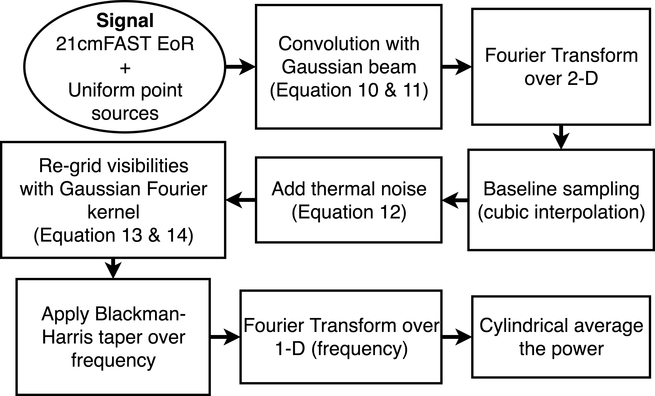
The full algorithm from §2.3.3 and 2.3.4 is summarized in Figure 1.

Figure 1: A summary of our instrumental algorithm.

2.4 Bayesian Parameter Estimation

Bayesian parameter estimation through Monte Carlo Markov Chain (MCMC) is a powerful algorithm that is widely used in a variety of scientific fields to constrain parameters of interest by determining their full posterior distribution. We have chosen to use 21cmMC, an MCMC analysis tool designed to estimate astrophysical parameter constraints from the EoR. It incorporates EoR simulation data produced on-the-fly by an optimized version of 21cmFAST to statistically compare the models to either mock or observed data (Greig & Mesinger, 2015).

The existing log-likelihood prescription used by 21cmMC uses the 1-D PS and is given by:

$$\ln\mathcal{L}=-\frac{1}{2}\sum_{j}\frac{(P_{D}(k_{j})-P_{M}(\theta,k_{j}))^{2}}{\sigma^{2}_{D}(k_{j})+(\alpha P_{M}(\theta,k_{j}))^{2}},$$ (17)

where $P_{D}$ is the 1-D PS of the experiment or mock data, $P_{M}$ is the model 1-D PS, $\theta$ is the set of EoR parameters for the model, $\sigma_{D}^{2}$ is the uncertainty of the experiment computed using 21cmSense (Pober et al., 2014), and $\alpha$ is a variable corresponding to the uncertainty of the model, often set to 10–20% by inspecting how close 21cmFAST is to radiative transfer models, with 15% being the default value. All estimates are a function of wavenumber, $k$. In the presence of foregrounds and the instrumental beam, this prescription is only optimal if the following set of conditions is satisfied:

1. The brightness temperature fluctuations are truly Gaussian

2. The EoR signal is 3-D isotropic

3. The sources of uncertainty have 3-D isotropic signal

4. The PS modes for both the EoR and foregrounds are Gaussian

5. The PS modes are independent for both the EoR and foregrounds

6. The foreground noise is independent of the EoR parameters.

We postulate that the first and second conditions are valid first-order assumptions and we leave the last one for future work. We discuss and address the others, along with a summary of our improvements to 21cmMC, in the following sub-subsections.

2.4.1 3-D Isotropic Uncertainties

The 1-D PS is employed because it provides complete information about the isotropic EoR signal. However, it confounds the impact of foregrounds because they naturally reside in a larger cylindrical Fourier space (i.e., smooth-spectrum versus angular clustering). In a 1-D PS, the wedge-mode contaminates the entire annulus because the foregrounds show a non-isotropic signature, corrupting some otherwise good modes. Although some sort of avoidance method is typically used to minimize the corruption of 1-D PS modes, it does not account for the full information.

We extend the likelihood formalism by using the 2-D PS instead of the 1-D PS as it allows for the management of systematic effects arising from $k_{\bot}$ and $k_{\parallel}$ modes respectively. The 2-D PS is commonly used as an initial step to decontaminate the cosmological EoR signal from the foregrounds in the forms of the “wedge” and the “EoR window”. Foreground power dominates the lower $k_{\parallel}$ modes, yielding higher variance in the wedge as compared to the EoR window. Using the 2-D PS means that modes in the same $|\vec{k}|$-annulus that may come from different $k_{\parallel}$ modes (from within and without the wedge) can be treated independently, and therefore the full information extracted.

2.4.2 Gaussianity and Independence of Instrument-Convolved Foregrounds

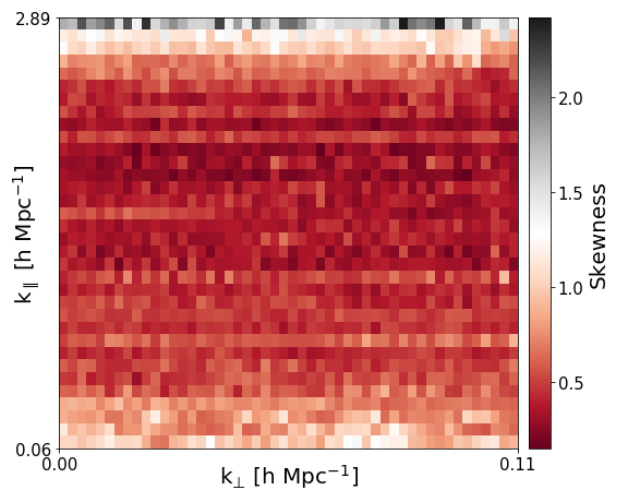
In Eq. 17, the use of $\sigma_{D}^{2}$ follows the assumption that the input data are Gaussian and independent. While this will hold true for the EoR signal since the cosmological signal is close to Gaussian, in the presence of foregrounds and instrumental effects, this assumption might break. We will focus on investigating the Gaussianity and independence of the instrument-convolved foregrounds because the variance of the data is dominated by the variance of the foregrounds in most bins. This can then dictate the appropriate formalism to adopt, without adding unnecessary complexity. Since we have established in the previous sub-section that we will be using the 2-D PS to accommodate the presence of foregrounds, we will continue this discussion using the 2-D PS of instrument-convolved foregrounds that were simulated based on our models; the ensemble is then used to compute the skewness and correlation in each 2-D mode.

We investigate the Gaussianity of the 2-D PS by finding the skewness in bins of $k_{\bot}$ and $k_{\parallel}$. The skewness measures the asymmetry of the probability distribution about its mean, with a skewness of 0 being perfectly symmetric and increasing skewness showing increasing asymmetry. Figure 2 shows the skewness of the 2-D PS of the instrument-convolved point source foregrounds. Over the primary range of interest (0.1 to 1 $h$ Mpc^-1), the bins are predominantly close to Gaussian. Regions of higher skewness are found only at either high $k_{||}$, where the signal is low, or low $k_{||}$, where the foregrounds are strong so the mode is therefore heavily down-weighted in the likelihood, and thus in our fits for the underlying parameters $\theta$. We are thus content to maintain the assumption of a Gaussian likelihood.

Figure 2: The skewness of the 2-D PS of the instrument-convolved point source foregrounds. The bins are predominantly close to Gaussian over the primary range of interest (0.1 to 1 $h$ Mpc^-1).

Figure 3: The correlation coefficient of the 2-D PS of the instrument-convolved foregrounds between a single cell with all other cells. The horizontal and vertical plots show cuts through the 2-D space at the chosen single cell locations, demonstrating the degree of correlation in the angular and line-of-sight modes. Each chosen ($k_{\bot},k_{\parallel}$) bin is completely correlated with itself (black cell in main panels corresponding to highest point in the smaller side panels). However, also note that the bin is highly correlated over $k_{\parallel}$ and the correlation spills over to the two $k_{\bot}$ bins adjacent to the chosen bin.

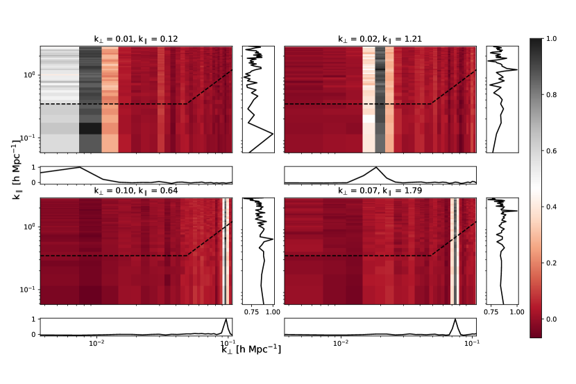
We investigate the assumption of independence of the instrument-convolved foreground model by finding the correlation coefficient between $k_{\bot}$- and $k_{\parallel}$-bins in the 2-D PS. The correlation measures the strength of the joint variability of two random variables, in this case the bins of $k_{\bot}$ and $k_{\parallel}$, with possible values ranging from -1 being completely anti-correlated to +1 being completely correlated. As with Gaussianity (cf. §2.4.2), we focus on the foregrounds rather than the 21 cm signal.

Figure 3 shows the correlation coefficient of the 2-D PS of the instrument-convolved foregrounds of four individual ($k_{\bot},k_{\parallel}$) bins with all other bins. The right- and bottom- sub-panels of each major panel show the correlation coefficient along a 1-D slice (in the displayed dimension) through the selected 2-D bin of each main panel. The dotted black line divides the area between the wedge and the EoR window. As expected, each chosen ($k_{\bot},k_{\parallel}$) bin is completely correlated with itself (black cell in main panels corresponding to highest point in the smaller side panels). However, we can also see that the bin is highly correlated over $k_{\parallel}$ and the correlation spills over to the two $k_{\bot}$ bins adjacent to the chosen bin. This is due to the frequency-dependence of the instrument, resulting in chromatic mode-mixing of foregrounds (Morales et al., 2012; Datta et al., 2010; Vedantham et al., 2012; Trott et al., 2012). As such, we can conclude that the 2-D PS of the instrument-convolved foregrounds is not independent between modes and that we must use the covariance, instead of the variance, in the likelihood prescription. Neglecting the dependence of the modes may result in over-constraining of parameters, regardless of whether the PS is is 1-D or 2-D.

We thus extend the likelihood prescription to use the multivariate normal likelihood, $\ln\mathcal{L},$ following the use of the 2-D PS and the presence of foregrounds. $\ln\mathcal{L}$ is given by

$$\ln\mathcal{L}=-\frac{1}{2}\left[\left(P_{D}-P_{M}(\vec{\theta})\right)^{T}\Sigma^{-1}\left(P_{D}-P_{M}(\vec{\theta})\right)\right],$$ (18)

where $\Sigma$ is the covariance of our fiducial noise and foreground ($N+FG$) model with the addition of sample variance (second term of following equation), so that the total variance, $\sigma^{2}_{T}$, is given by

$$\sigma^{2}_{T}=\sigma^{2}(P_{N+FG;M})+\frac{P_{21;M}^{2}}{\sum_{j}(\sum\limits_{i=0}^{N_{\rm bl}}w_{i})^{2}};$$ (19)

$$P_{D}=P_{D}(k_{\bot},k_{\parallel})=P_{21+N+FG;D}$$ (20)

is the (mock) data PS, assumed to be comprised of a 21 cm component, and a noise and foreground component; and

$$P_{M}(k_{\bot},k_{\parallel}|\vec{\theta})=P_{21}(k_{\bot},k_{\parallel}|\vec{\theta}_{21})+P_{N+FG}(k_{\bot},k_{\parallel}|\vec{\theta}_{N+FG})$$ (21)

is a parameter-dependent model of the data. Note that we use the expected power of noise and foregrounds instead of just one specific realization for the model. Because it is computationally-expensive and difficult to calculate the expected power of all components at each iteration, we have modelled the 21 cm signal separately and use the same expected foregrounds and noise power each time, which is possible because we do not have $\theta_{N+FG}$ parameter in the likelihood. This also assumes that the cross-power terms are negligible and is a reasonable first-order approximation consistent with other works; however, we will see in §5 that this assumption is not true.

Note that $P_{D}$ and $P_{M}$ are not the true power spectrum computed from the simulation box. They are related to the true power spectrum, $P^{*}$, by $P=\hat{W}P^{*}$ where $\hat{W}$ is all the window functions that encompasses the instrumental and analysis effects such as the beam and frequency taper used in this research. The fact that we compute $P_{D}$, $P_{M}$, and $\Sigma$ using exactly the same pipeline means that they are self-consistent hence the effects of $\hat{W}$ should cancel out in the likelihood. Also note that the form of Eq. 18 explicitly assumes that the covariance does not depend strongly on the astrophysical parameters. Otherwise, it would require an extra term of $-\ln{\rm det}(\Sigma^{-1})$. This is a reasonable assumption for most cylindrical $k$-modes which are dominated by foregrounds whose parameters we are not directly interested in.

2.5 Extensions to 21cmMC

The foregrounds and instrumental components, along with other improvements developed in this work and described in the previous sections, are combined in a publicly-available plug-in to the new 21cmMC, called py21cmmc-fg. It makes use of 21cmMC’s new ability to allow the user to arbitrarily insert code to modify the lightcone before producing a likelihood. This creates realizations of the EoR signal obscured by the foregrounds which are measured by an instrument model and then used as input to the log-likelihood.

To summarise, the extensions to 21cmMC that are available in py21cmmc-fg include:

• a foreground model: includes both diffuse and point-source foregrounds (although only the latter is used in this work for simplicity)

• an instrument model: includes a Gaussian beam model, the array baseline sampling and thermal noise

• calculation of the 2-D PS: to separate the cosmological EoR signal from the foregrounds

• the covariance of the PS: to account for the correlated instrument-convolved foregrounds

• the likelihood prescriptions for the MCMC: expand to multivariate normal distribution

• stitching of the lightcones: to account for the wide FOV of the instrumental beam model

• padding of the sky: to increase the image resolution for Fourier Transform

• Fourier beam gridding kernel: to properly interpolate, average and weight visibilities onto a grid

All of these have been discussed in detail in this section, except for the stitching of the lightcones. We will discuss this in the next section (§3) when we explore the observational effects on the EoR lightcones.

2.6 Comparison to Existing Framework

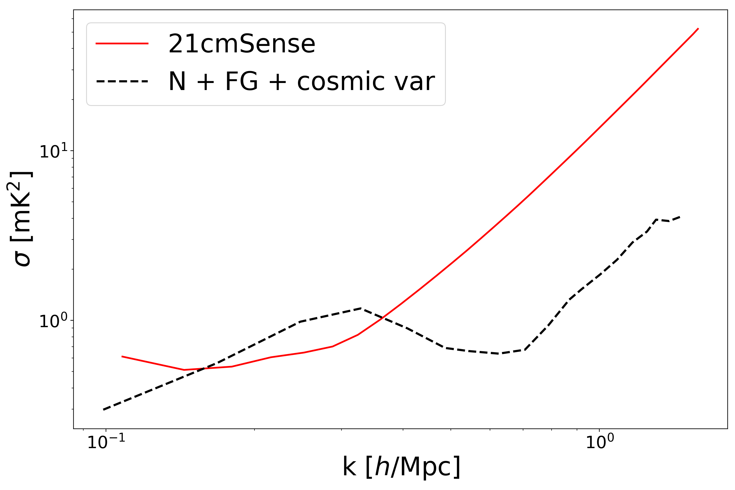
The final focus of this section is to compare the uncertainty level from our framework, py21cmmc-fg, to that from the publicly-available existing framework, 21cmSense (Pober et al., 2013, 2014). In general, 21cmSense performs a separate calculation of the instrument sensitivity arising from thermal noise and cosmic variance while avoiding the foreground-dominated region; the uncertainty file is then used as input into 21cmMC . For more details, we refer readers to Pober et al. (2013) and Pober et al. (2014).

For 21cmSense, we adopt the drift scan mode and “moderate” foreground removal with the MWA Phase II baselines, $A_{\rm eff}=21$ m² and $T_{sys}=240$ K. We also use $\Delta t=2\times 10^{5}$ hours in both frameworks. The reasoning behind this value is explained in detail in §4, but in general, we use this value so that we can approximate the noise level for 1000 hours observation of the future SKA_LOW1.

Note that the uncertainty with sample variance is calculated differently in the two frameworks. Our framework calculates $\sigma^{2}_{T}$ based on Equation 19, while 21cmSense defines $\sigma^{2}_{T}$ as

$$\sigma^{2}_{T}(k)=\left(\sum_{i}\frac{1}{(P_{21}(k)+P_{N,i}(k))^{2}}\right)^{-\frac{1}{2}},$$ (22)

whereby an inverse-weighted summation is performed over the $uv$ cell $i$ for each $k$ mode bin (Pober et al., 2013). The main difference between the two frameworks is the presence of the cross-terms between the EoR PS and the noise variance for 21cmSense.

In addition to the calculation of sample variance, 21cmSense and py21cmmc-fg have a few key differences that can affect the total uncertainty level. We have summarized these differences in Table 2. The resulting total uncertainty from the two frameworks are presented in Figure 4. The total uncertainties loosely match at the relevant modes where the signal dominates, with a difference of less than half an order of magnitude. At high $k$, however, the difference is as high as one order of magnitude. We attribute the difference in total uncertainty to the missing Earth rotation synthesis which essentially fills up more $uv$ space hence increasing the overall noise level (i.e., less modes can combine coherently). Even though the Fourier beam gridding kernel we employ partly takes this into account, it does not restore the noise to the full level that it would be with a proper rotation synthesis. We note that this is a shortcoming of our framework, and is left for future work.

	21cmSense	py21cmmc-fg
PS	1-D	2-D
Frequency-dependent baselines	No	Yes
Cross-power in variance	Yes	No
Foregrounds	Avoidance	Suppression
Earth rotation synthesis	Yes	No
Baseline sampling on EoR PS	No	Yes
Frequency taper	No	Yes
Gridding kernel	No	Yes

Table 2: The differences between 21cmSense and py21cmmc-fg.

Figure 4: The total uncertainty from 21cmSense (red solid line) compared to the total uncertainty from our framework (black dash line) with $T_{sys}=240$ K and $\Delta t=$ 2$\times 10^{5}$ hours.

3 Observational Effects on EoR Lightcones

Figure 5: Comparison of the 1-D PS of the 7.5 Gpc box (red), the stitched 1.5 Gpc box (green dotted), and the stitched 1.5 Gpc coarsened to a resolution of 15 Mpc (blue dash-dot). The 7.5 Gpc box and the stitched 1.5 Gpc box agree very well on most scales, but the 1-D PS of the stitched and coarsened box differs from the 1.5 Gpc box at high $k$ due to finite resolution.

In this section, we explore the observational effects of adding foregrounds to the EoR signal. This is first done by explaining the steps we have taken to ensure that both the EoR signal and foregrounds can be added together. We then analyse the effects on the 1-D and 2-D power spectra and compare the differences in image space.

In order to add the foreground and EoR lightcones, they need to cover the same angular size and have the same angular resolution. At $z=6$, the resulting angular sky size of a 1 Gpc$/h$ simulation box, which is considered to be large in theoretical studies, is merely $\sim 0.12$ radian. On the other hand, the FOV of the MWA is $\sim 1$ radian. Running a massive box that covers the MWA FOV is unrealistic and computationally expensive, so instead, we have made a realization of the lightcone across the mock sky by assuming that the same structure is periodically repeated. To preserve the wavenumber, we have ensured that the full box is used in the stitching i.e., we use an integer number of boxes. We also limit ourselves to using scales smaller than the box size in the parameter estimation to avoid systematics due to this repetition.

Furthermore, due to memory-limitation, we have opted to coarsen the EoR signal using interpolation. Of course, the coarsening process can be avoided by setting the EoR lightcone from 21cmFAST to be of the same angular size. This, however, will affect the small-scale processes involved in determining $\delta T_{b}$, so we prefer to perform the coarsening post-stitching.

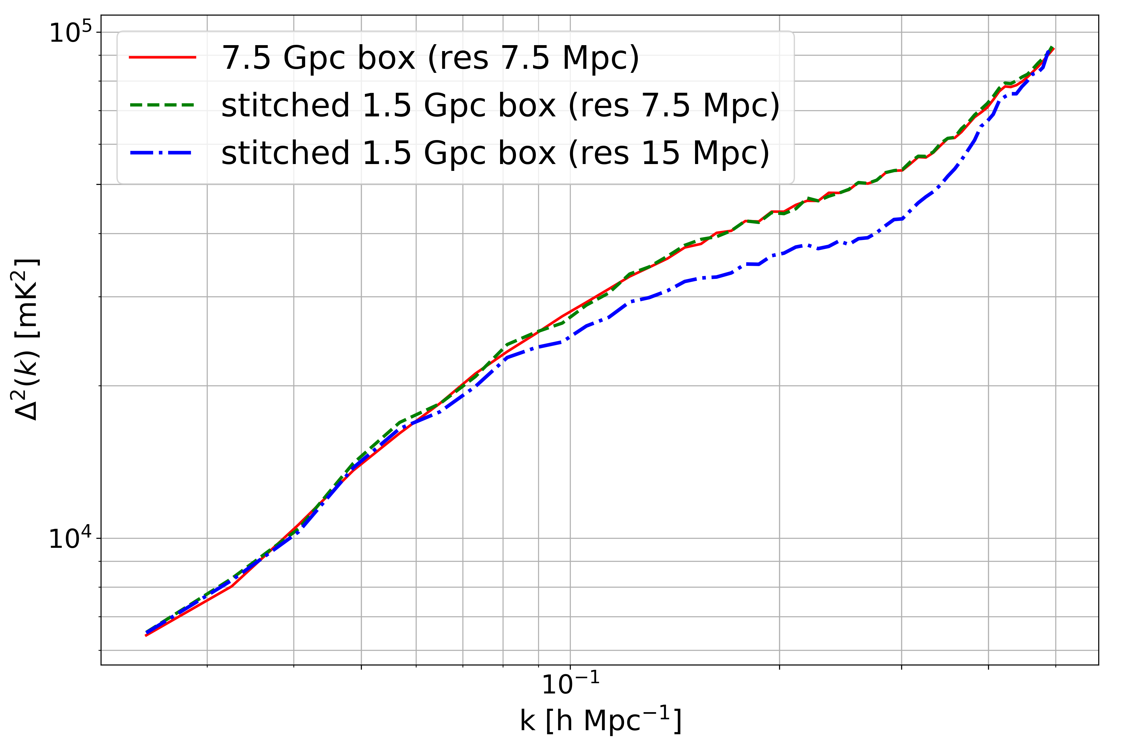
To study the effects of tiling and coarsening of the lightcone, we use simulation boxes of size 1.5 and 7.5 Gpc, both with a resolution of 7.5 Mpc. While we will typically work with the 2-D PS, we use the 1-D PS when comparing data quantitatively in this section. We compare the 1-D PS of the 7.5 Gpc box, the stitched 1.5 Gpc box, and the stitched 1.5 Gpc coarsened to a resolution of 15  Mpc in Figure 5. The $y$-axis shows the dimensionless 1-D PS while the $x$-axis shows the $k$ scales.

The 7.5 Gpc box and the stitched 1.5 Gpc box agree very well on most scales, suggesting that stitching the box does not negatively affect the PS. However, the 1-D PS of the stitched and coarsened box differs from the 1.5 Gpc box at high $k$. This is, of course, expected as the coarsening of the box results in a different resolution, hence affecting the small scale structure of the $\delta T_{b}$. The stitching of boxes and coarsening of the resolution may potentially affect the statistics of the PS due to lack of cosmic variance.

Herein, we have been presenting plots in cosmological units. In the code and hereafter in the paper, we have opted for observation units of Jy, Hz and radians to minimise inconsistencies and errors in converting between the two units. Note that the choice of units is inconsequential for the likelihood, as long as the same units are used in numerator and denominator.

4 MCMC Analysis

Figure 6: A corner plot comparing the constraints our systematic tests: uniform $uv$ sampling with no thermal noise or foregrounds (blue); uniform $uv$ sampling with point-source foregrounds but no thermal noise (orange); uniform $uv$ sampling with 1000 hours of thermal noise with the MWA but no foregrounds (green); MWA baseline sampling with $2\times 10^{5}$ hours of thermal noise with the MWA but no foregrounds (red); MWA baseline sampling with $2\times 10^{5}$ hours of thermal noise with the MWA and point-source foregrounds (purple). The use of $2\times 10^{5}$ hours of thermal noise with the MWA is comparable to the noise level of 1000 hours with the SKA. The artificial “uniform” $uv$ sampling unnecessarily inflates the impact of thermal noise (green) as it restricts the number of baselines per $uv$ cell to one and the small collecting area of the MWA gives a signal-to-noise ratio of order unity; both of these factors results in a biased estimate. With the addition of baselines sampling and the use of SKA sensitivity, the constraints are remain unbiased (purple and red) although the final test (red) gives a really inflated constraint compared to the other tests. Note that these constraints still have the burn-in phase included.

For parameter estimation, we use an EoR lightcone of size 750 $h^{-1}$Mpc with 250 cells. The lightcone is stitched together to cover 1 steradian of the sky and coarsened to 800 cells (resolution of $\approx$ 24 $h^{-1}$Mpc) before being padded by zeros to 3 times the sky size to increase the resolution for the Fourier Transform. The bandwidth of the observation is 10 MHz from 150 to 160 MHz with 100 frequency channels. We assume that $T_{sys}=240$ K, corresponding to the average sky temperature at 150 MHz.

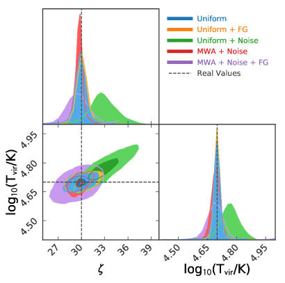
To ensure that our MCMC framework is consistent, we first perform simpler tests in which we attempt to loosely constrain only two parameters, $\zeta$ and $T_{vir}$ (with fiducial values of $\zeta$=30.0 and $T_{vir}=4.7$  log₁₀K). These systematic tests include:

1. Uniform – regular and filled – $uv$ sampling with no thermal noise or foregrounds

2. Uniform $uv$ sampling with point-source foregrounds but no thermal noise

3. Uniform $uv$ sampling with thermal noise but no foregrounds

4. MWA baseline sampling with thermal noise but no foregrounds

5. MWA baseline sampling with thermal noise and point-source foregrounds

Step 5 constitutes the end-goal of this work (but with all four parameters from Table 1). Note that with these tests, we are not interested in properly estimating the values of the parameters; we only want to gauge whether the MCMC walkers would assemble around the right values, thereby the burn-in phase of the walkers are still included in this section. We initially set the observation time to 1000 hours consistent with other research, but the observation time is later increased to 2$\times 10^{5}$ hours (the motivation of which is explained later in this section). To clarify, only steps 1 - 3 are done with 1000 hours of observation time. The final two steps, along with everything else after, are done with 2$\times 10^{5}$ hours.

We present a corner plot of our checks in Figure 6, which shows the projection of the values of the parameters over 1-D and 2-D space density. The black dash lines show the actual value of the parameter while the colored, shaded regions show the values of the estimated parameter that have been projected over the density space in 1-D (diagonal plots) and 2-D (non-diagonal plots).

It is clear that convolving the stitched and coarsened EoR signal with the Gaussian beam and implementing the 2-D PS and the multivariate normal distribution in the likelihood prescription do not negatively impact the parameter estimation, as apparent from the constraints from Step 1 (blue region). The addition of point source foregrounds in Step 2 (orange) does not significantly expand the constraints. This can be attributed to the fact that the foreground contamination is fully contained at smaller $\eta$ due to the uniform $uv$ sampling.

Figure 7: The power spectra of the EoR signal (left) and the thermal noise with the MWA sensitivity (right) in unit of Jy²Hz². With the uniform $uv$ sampling, the signal to noise ratio is of order unity for 1000 hours of observation time due to the small collecting area of the MWA. While this is enough for an EoR signal detection over the slope of the 1-D PS, it is not sensitive enough for EoR parameter estimation with the MWA.

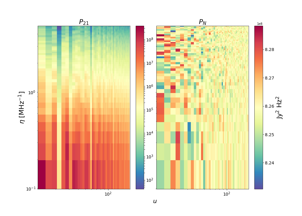
However, with the addition of thermal noise in Step 3 (green region), the peak of the distribution is significantly shifted with respect to the true value, indicating that the results are biased. We note also that the artificial “uniform” $uv$ sampling unnecessarily inflates the impact of thermal noise, as it restricts the number of baselines per $uv$ cell to one. To investigate the cause of the bias, we plot the 2-D PS of the EoR signal and the thermal noise, presented in Figure 7. With the uniform $uv$ sampling, the signal-to-noise ratio is of order unity for 1000 hours of observation time due to the small collecting area of the MWA, either with the MWA baselines sampling or the uniform $uv$ sampling. While this is enough for an EoR signal detection over the slope of the 1-D PS, it is not sensitive enough for EoR parameter estimation with the MWA.

To enable parameter constraints for the remainder of the work, we henceforth increase $\Delta t$ in Equation 12 to 2$\times 10^{5}$ hours for the MWA-based instrument model that we have. This $\Delta t$ is equivalent to adopting an SKA-like sensitivity for which $A_{\rm eff}=300\,{\rm m}^{2}$ but is achievable with only 1000 hours. As seen in Step 4 (red region), both the use of the larger collecting area and the presence of $uv$ sampling reduces the noise, resulting in the MCMC converging to the model values.

In Step 5 (purple region), the presence of point source foregrounds expands the posteriors by 100% compared to thermal noise alone without bias. The reason the purple contour is larger than the red, while the orange is not larger than the blue, is that non-uniform sampling implies chromaticity which creates the wedge, and therefore removes a lot of otherwise useful modes.

5 Parameter Estimation Results

Figure 8: An example trace plot from the 160–170 MHz band with thermal noise and foregrounds. The blue lines show the true value of the parameter while the black lines show the progression of the parameter estimation at each iteration. In this particular case, we have ignored the walkers with $\ln\mathcal{L}<-4000$.

Now that we have established the robustness of our additional model complexities, we can use the MWA baseline sampling with thermal noise and point-source foregrounds to constrain the four reionization parameters in Table 1. We use three different frequency bands: 150–160, 160–170, and 170–180 MHz to observe the EoR signal, which is obscured by point-source foregrounds in the presence of instrumental effects and thermal noise.

Before we proceed with our results, we would like to emphasize that our pipeline is computationally intensive and time-consuming. With 5 chains run for each parameter, we have 20 walkers in total. One iteration per walker uses 10 GB of memory per node and takes roughly 20 minutes to completely simulate the EoR brightness temperature field, tile and coarsen it to cover the whole sky, add a Gaussian beam, Fourier Transform the beam-convolved sky and sample the $uv$ sample, re-grid the visibilities and cylindrically average them to find the 2-D PS before finding the log-likelihood. The bottleneck of our pipeline is in re-gridding the visibilities using a Gaussian beam kernel after baseline sampling, which takes around 15 minutes to complete.

To test the performance, we use a Gaussian Process model to fit for the maximum likelihood autocorrelation function which is used to estimate the autocorrelation time, $\tau$. We found that $\tau\approx 200$ iterations irrespective of which frequency band is being used, with the recommended total iteration being 50$\tau$. However, because of the memory and time limitations we have mentioned above, we have only run our chains up to around $5\tau$. This is not enough to definitively claim that our chains have properly converged, but the results we currently have are useful to give an initial estimate of how well we can constrain the EoR parameters in the presence of foregrounds and thermal noise with our pipeline and gauge the plausibility of our assumptions.

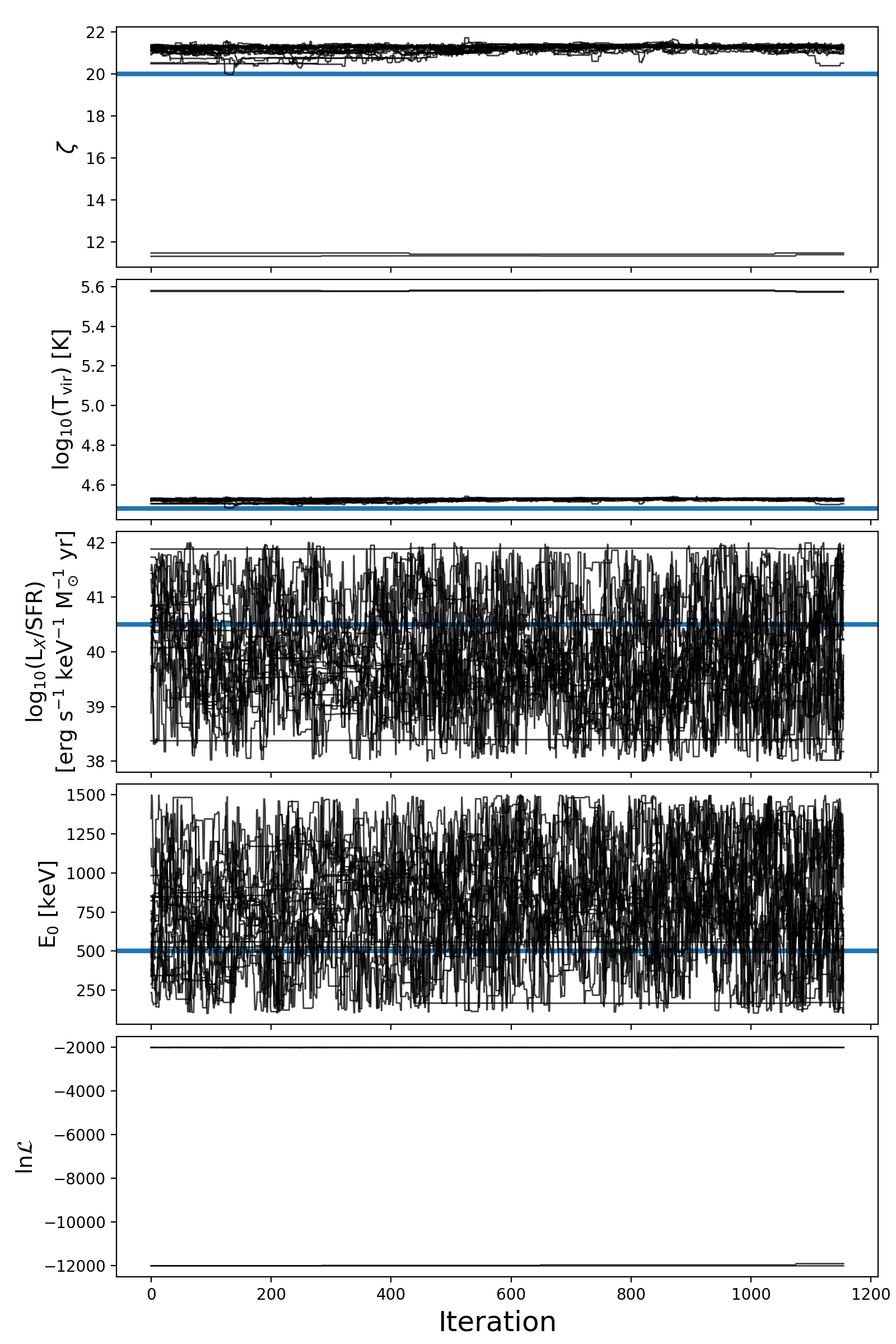
Furthermore, in calculating our constraints, we have ignored walkers that are stuck in local minima. An example of this is shown in Figure 8, where we have plotted the trace plots which show the values of the four EoR parameters at every iteration and the corresponding $\ln\mathcal{L}$ after burn-in for the 160–170 MHz band with thermal noise and foregrounds. In this particular case, we have ignored the walkers with $\ln\mathcal{L}<-4000$.

Figure 9: A corner plot comparing the constraints of EoR parameters in the presence of instrumental noise and foregrounds in the different frequency bands: 150–160 (orange), 160–170 (green), and 170–180 (blue)  MHz.

Figure 10: The 2-D power spectra of the EoR signal (i.e. without foregrounds or thermal noise) in the 160–170 MHz band for the true values (left) and the MCMC values (middle) – the median values of $\zeta=21.13$, log${}_{10}(T_{vir})=4.52$ , L_X/SFR = 40.00, and E₀=0.656 keV– along with their ratio. The true parameters give a maximum power that is up to 6 times higher than the MCMC parameters in the EoR window, suggesting that it is deceptively easy to discriminate between the two models.

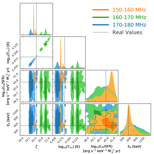
We present a corner plot of the different observation bands in Figure 9 in which the orange, green, and blue shaded regions represent the 150–160, 160–170, and 170–180 MHz bands respectively. The black dashed lines show the true values of the parameters ($\zeta=20$, log${}_{10}(T_{\rm vir})=4.48$ , L_X/SFR = 40.5, and E₀=0.5 keV). The darker/lighter shaded regions represent 1$\sigma$/2$\sigma$ confidence regions corresponding to the 84^th and 16^th percentiles. From the figure, it is clear that L_X/SFR and $E_{0}$ are relatively unconstrained in all frequency bands and that $T_{\rm vir}$ is tightly constrained. Note that $\zeta$ and $T_{vir}$ are quite correlated and biased in all bands. This is especially true for the 160–170 MHz band in which the green region is further from the truth values. The bias suggests that the primary effects of $\zeta$ and $T_{vir}$ are on regions which are most affected by foregrounds on the larger scales. A bias indicates either a very anomalous noise realization (more than 2 sigma over the whole 2D parameter space), or an incorrect model.

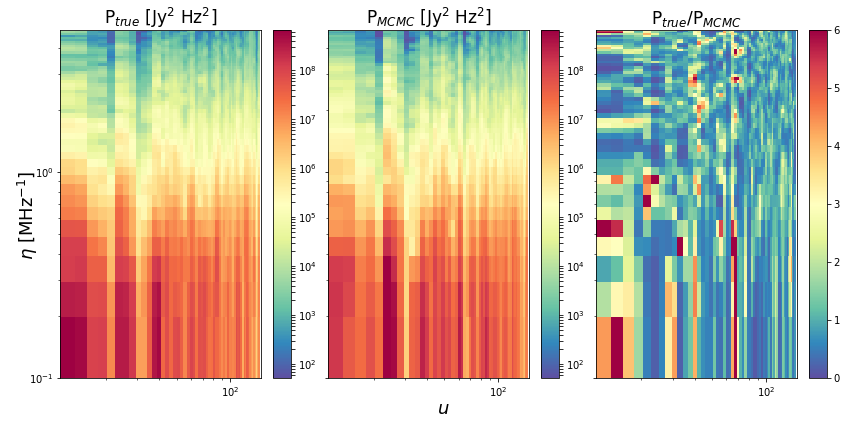
To investigate the reason for the bias in the presence of foregrounds, we present the 2-D power spectra of the EoR signal (i.e. without foregrounds or thermal noise) in the 160–170 MHz band for the true values and the MCMC values – the median values of $\zeta=21.13$, log${}_{10}(T_{vir})=4.52$ , L_X/SFR = 40.00, and E₀=0.656 keV– along with their ratio in Figure 10. The true parameters give a maximum power that is up to 6 times higher than the MCMC parameters in the EoR window, suggesting that it is deceptively easy to discriminate between the models.

Figure 11: The 2-D power spectra of the data i.e. EoR signal, foregrounds and thermal noise (left) and the EoR signal (middle) in the 160–170 MHz band along with their difference (right). The negative power (white region) in the right panel is caused by the unaccounted contribution of the cross-power terms between the EoR signal and the foregrounds and thermal noise.

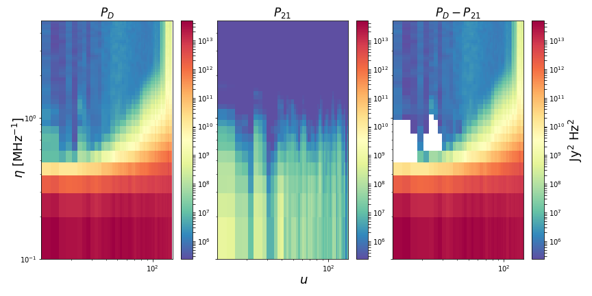
In reality, however, it should be considered that the presence of foregrounds and noise may obscure modes that are vital for differentiation of these models. Figure 11 shows from left to right: the 2-D PS of the data i.e. the EoR signal, thermal noise and point source foregrounds, the 2-D PS of the true EoR signal and the difference between these two. The negative power in the right panel is caused by the unaccounted contribution of the cross-power terms between the EoR signal and the foregrounds and thermal noise. This is because the EoR signal and the expected thermal noise and foregrounds are modelled separately as mentioned in §2.4.

We can estimate cross-power by looking at the variance of the difference between the 2-D power spectra of the data ($P_{D}$) and the model ($P_{M}$) for a single realization of 21cm power spectrum but with an ensemble of foregrounds and noise realizations following

$$\textrm{Var}(P_{D}-P_{M}) =\rm Var[\langle|(V_{21}+V_{FG}+V_{N})|^{2}\rangle_{\textbf{u}}$$

$$-\langle|(V_{FG}+V_{N})|^{2}+|(V_{21})|^{2}\rangle_{\textbf{u}}]$$

$$=\langle 2P_{21}[\textrm{Var}(V_{FG})+\textrm{Var}(V_{N})]\rangle^{*}_{\textbf{u}},$$ (23)

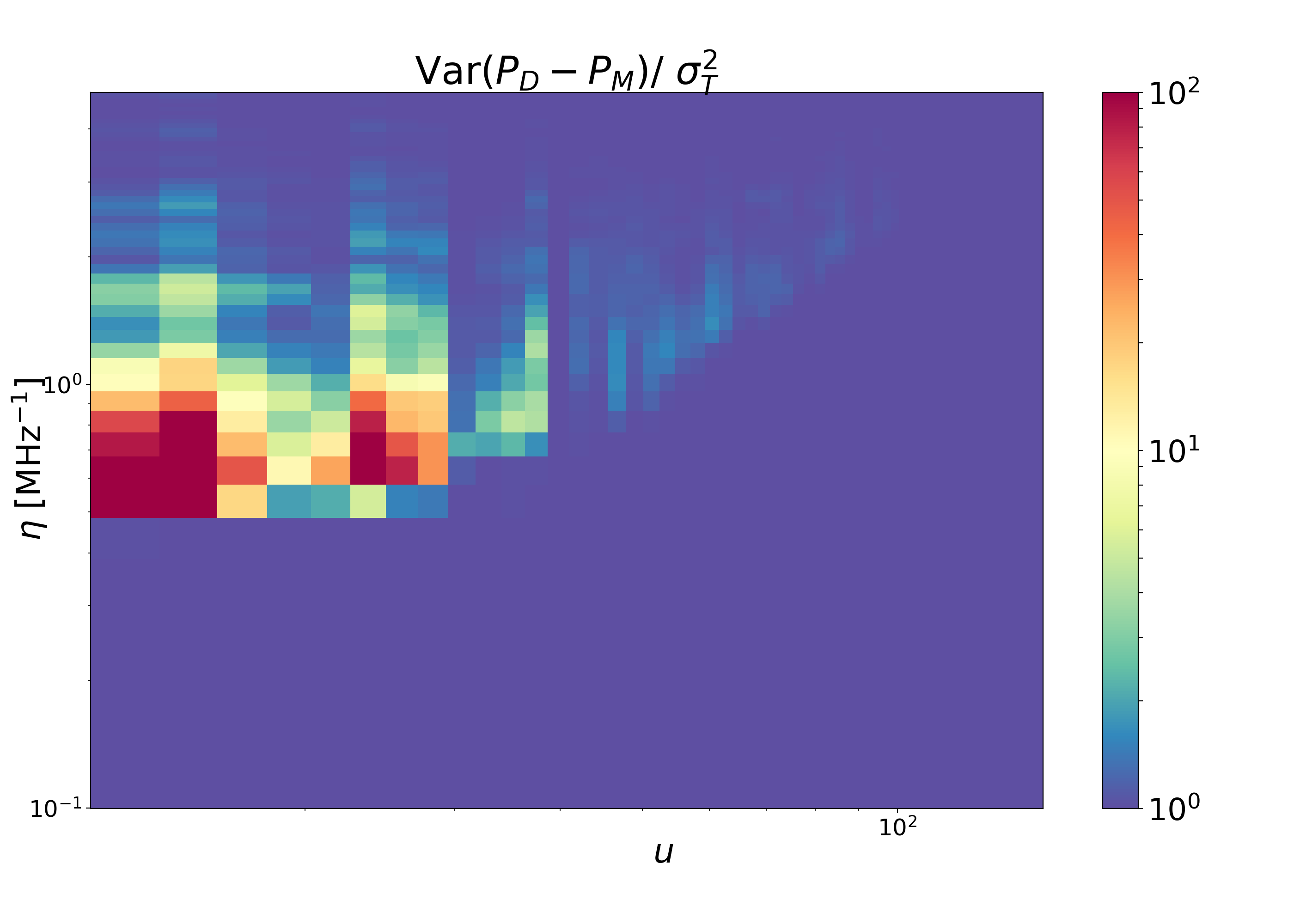
where $V_{21}$, $V_{FG}$, and $V_{N}$ are the visibilities of the EoR signal, foregrounds and noise respectively. For simplification, $\langle$ $\rangle_{\textbf{u}}$ denotes the cylindrical average in u bin with weighting as described in §2.3 and $\langle$ $\rangle^{*}_{\textbf{u}}$ is the same as $\langle$ $\rangle_{\textbf{u}}$ except the weighting is squared; see the appendix for the complete derivation. From the equation, we can see that the variance is largest when $P_{21}$ is larger than the noise and foregrounds. To investigate this further, we present the ratio of the variance of $P_{D}-P_{M}$ and the true total variance $\sigma_{T}^{2}$ in Figure 12. The region that is more correlated than the other modes is at u $\leq 30$, whereby the size of the correlated bins are dictated by the correlation lengths of the window functions. This is evident from the red regions in the figure which extend over 2u by 4$\eta$ bins, corresponding to the correlation length of the MWA following $D/\lambda$ and the Blackman-Harris taper respectively.

Figure 12: The ratio of the variance of the $P_{D}-P_{M}$ to the actual total variance, $\sigma_{T}$.

To further explore the region where most of the biasing takes place and gauge the net effect of the cross-power on the likelihood, we calculate the pseudo-likelihood ($\mathcal{\hat{L}}$) given by

$$\mathcal{\hat{L}}=-\frac{(P_{D}-P_{M})^{2}}{\sigma_{T}^{2}}.$$ (24)

This is a variation of Equation 18 but with $\sigma_{T}^{2}$ instead of $\Sigma$. Figure 13 show -$\mathcal{\hat{L}}$ for the true (left) and MCMC (right) parameters. -$\mathcal{\hat{L}}$ is overall greater for the true parameters, as apparent from the overwhelming red region in the left panel. This region coincides with low u, thus supporting our argument that this region is more correlated. With realistic datasets whereby the visibilities from the different components are summed before the PS is calculated, the likelihood has biased signal discrimination power when the same steps are not taken for the model. The likelihood favours whichever EoR model that accounts for the cross-power term thus resulting in biased constraints.

Figure 13: -$\mathcal{\hat{L}}$ for the true (left) and MCMC (right) parameters. -$\mathcal{\hat{L}}$ is overall greater for the true parameters, as apparent from the overwhelming red region in the left panel coinciding with low u.

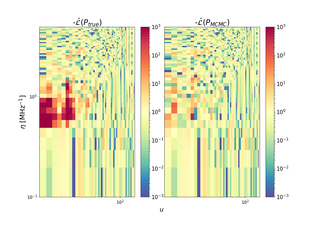
In principle, the signal to noise ratio is greater than one in every PS cell outside the wedge because of our low level of thermal noise. This results in the use of all modes of the PS in calculating the likelihood, including the ones that do not have any real constraining power, i.e. less signal. In addition, because the signal is stronger at modes with u$\leq 30$, these modes are more affected by the subtle cross-correlation effects from noise and foregrounds. The deficits in the modelling can thus lead to biased answers as the likelihood tries to compensate for the missing power.

Because our MCMC runs are shorter and may have not properly converged, the constraints from the MCMC may be invalid. To sample the “true” $1\sigma$ contours for a Gaussian posterior, we explore the $\Delta\chi^{2}$ contours by assuming that the true $\chi^{2}$ value is identical to the degree of freedom ($df$) (hence the $1\sigma$ level is $\sqrt{2df}$).

Figure 14: The $\Delta\chi^{2}$ contours for the three bands using the best fitting parameters from our framework which are presented in Table 3. With $df=2996,$ the $1\sigma$ level is $\sim 77$. Because the constraints for L_X/SFR and E₀ from the MCMC look reasonably inflated, we only focus on examining the $\Delta\chi^{2}$ contours for $\zeta$ and $T_{\rm vir}$.

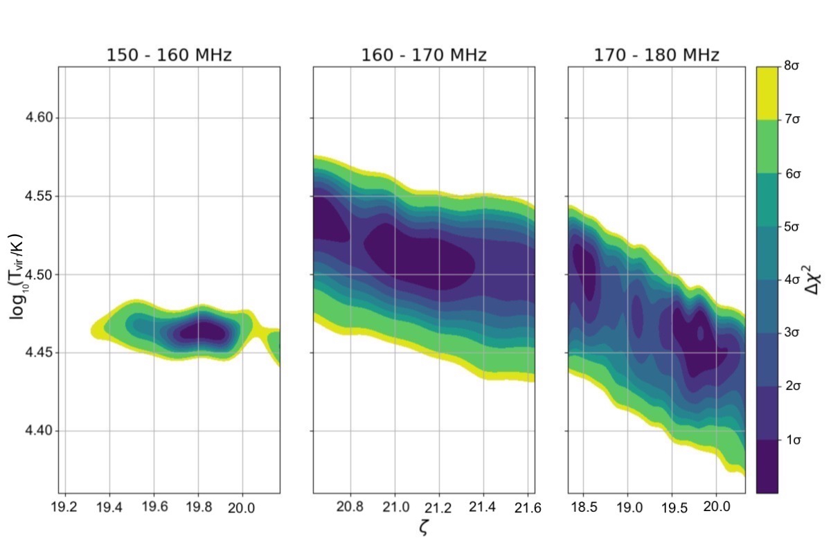
In Figure 14, we present the $\Delta\chi^{2}$ contours for the three bands using the best fitting parameters from the MCMC results shown in Figure 9. With $df=2996,$ the $1\sigma$ level is $\sim 77$. Because the constraints for L_X/SFR and E₀ from the MCMC look reasonably inflated and unbiased, we focus on examining the $\Delta\chi^{2}$ contours for $\zeta$ and $T_{\rm vir}$.

We see that there are multiple regions in the parameter space that satisfy the $1\sigma$ condition in the middle and last frequency bands. This can confound the parameter estimation via MCMC. Additionally, we can see that the constraints for $T_{\rm vir}$ are not as tight as shown in Figure 9 but the constraints for the other parameters match the results from the MCMC.

We present the estimated median values of the parameters from each of the MCMC runs in Table 3, with the upper and lower limit being the 1$\sigma$ level from the $\Delta\chi^{2}$ grid. In the presence of both foregrounds and thermal noise, $T_{\rm vir}$, L_X/SFR and E₀ are all within 1$\sigma$ from the truth for the three frequency bands. For $\zeta$, however, the best fitting parameter values are off by as much as $5\sigma$ due to the unaccounted cross-power terms. This suggests that the effects of $\zeta$ on the PS space are primarily at low u region, since these modes are significantly impacted by the missing power.

		150 - 160 MHz	160 - 170 MHz	170 - 180 MHz
$\zeta$	20	$19.67^{+0.23}_{-0.00}$	$21.13^{+0.18}_{-0.23}$	$19.33^{+0.77}_{-0.00}$
log${}_{10}(T_{vir}$)	4.48	$4.47^{+0.01}_{-0.00}$	$4.52^{+0.01}_{-0.04}$	$4.46^{+0.04}_{-0.03}$
log${}_{10}(L_{X}/$SFR)	40.5	$40.09^{+0.48}_{-1.19}$	$40.00^{+0.99}_{-0.92}$	$40.22^{+0.94}_{-1.06}$
E0	500	$531.51^{+209.64}_{-34.39}$	$656.50^{+409.39}_{-242.44}$	$739.60^{+385.11}_{-348.29}$

Table 3: Results of astrophysical parameter constraints from the MCMC for the different frequency bands and with different components. The upper and lower limit show the 1$\sigma$ level from the $\Delta\chi^{2}$ grid.

6 Discussion and Conclusion

Our 21cmMC plug-in, py21cmmc-fg, simulates statistical point-source foregrounds and instrumental components that include a Gaussian beam, $uv$-sampling and thermal noise. It uses a Gaussian Fourier beam to re-grid the data before spherically averaging it to compute the 2-D PS. The 2-D PS allows for the use of the entire parameter space in the likelihood computation, effectively ensuring that the effects of foregrounds are accounted for, even in the EoR window.

We show that the implementation of a multivariate normal likelihood and the covariance of the noise and foregrounds appropriately down-weights modes that are contaminated by foregrounds, thus optimally accounting for all Gaussian information. Additionally, the low level of noise ensures that all modes in the EoR window are used in calculating the likelihood, even though not all modes actually have constraining power. Due to incomplete sampling of the posteriors and insufficient convergence of the chains, a cross-check with a Gaussian posterior distribution is needed to properly constrain the parameters.

Furthermore, in order to accurately constrain the parameters, it is imperative that future experiments take into account the cross-power terms between the EoR signal and the foregrounds and noise. This can be done by either properly modelling all the components together, or by quantifying the cross-power terms separately and adding it to the framework we have developed. Nevertheless, both of these approaches may be computationally expensive and require a lot of memory because the gridded visibilities from all the foregrounds and thermal noise runs need to be stored and added to the EoR signal on each iteration.

Though our research does not address the full complexity of 21 cm parameter estimation experiments, it is the first step towards a more realistic one. In the future, however, it would be useful to include:

• Earth rotation synthesis;

• the full curved-sky visibility equation, including the $w$-term particularly for the MWA;

• more realistic, non-Gaussian beams, including non-analytic ones such as the MWA beam (Sutinjo et al., 2015);

• multi-redshift parameter estimation;

• other systematics such as RFI, ionosphere, gain errors and cable reflections;

• diffuse Galactic foregrounds;

• clustered extragalactic point-source foregrounds; and

• uncertain foreground parameters.

Out of all these effects, the inclusion of Earth rotation synthesis and Galactic foregrounds are the most important because they can lead to a higher noise level up to 3$\times$ for longer baselines, as shown by 21cmSense, and contain spatially-structured signal, for the latter. Moreover, a further optimization of the code is necessary for more accurate constraints and absolute convergence of the MCMC.

Appendix A Fourier Conventions

The Fourier Transform (hereafter FT) conventions used in this paper are as follows. The continuous $n$-dimensional FT, $F(\textbf{k})_{\infty}$, can be written as

$$F(\textbf{k})_{\infty}=\sqrt[n]{\frac{|b|}{(2\pi)^{1-a}}}\int f(\textbf{r})\exp(-ib\textbf{k}\cdot\textbf{r})d^{n}\textbf{r},$$ (A1)

where r is the comoving coordinate in real space, k is the Fourier dual of r, and $a$ and $b$ are arbitrary constants (Murray, 2018). Conventionally, radio interferometry uses $(a,b)=(0,2\pi)$, while cosmology uses $(a,b)=(1,1)$. To approximate a continuous FT, a discrete FT normalises by the physical length of the data set ($L$) per number of data available for each dimension ($N$). The resulting modes, $k$, measured from the transform are

$$k=\frac{2\pi}{b}\frac{m}{L},m\in(-N/2,...,N/2).$$ (A2)

Appendix B Variance of Residual

Let $w_{i}$ be the weights used in averaging from 3D $(u,v,\eta)$-space down to 2D $(u,\eta)$-space, and $N^{u}_{uv}$ is the number of UV cells in a given $|u|$ bin; the variance of $P_{D}$ is thus

$$\rm{Var}(P_{D}) =\frac{\sum_{i\in uv}^{N^{u}_{uv}}w_{i}^{2}\rm{Var}(\mathcal{Q})}{\left(\sum_{i\in uv}^{N^{u}_{uv}}w_{i}\right)^{2}}$$

$$\equiv\langle\rm{Var}(\mathcal{Q})\rangle^{*}_{\textbf{u}},$$

where

$$\mathcal{Q}=V_{21}V^{\dagger}_{21}+V_{FG}V^{\dagger}_{FG}+V_{N}V^{i\dagger}_{N}+2\mathcal{R}e(V_{21}V^{\dagger}_{FG}+V_{21}V^{\dagger}_{N}+V_{FG}V^{\dagger}_{N}).$$ (B1)

In our case, while both $V_{\rm FG}$ and $V_{N}$ are complex random variables, $V_{21}$ is not random. We use the same random seed to create the signal that comprises the mock data and all the model realizations throughout the MCMC (though these have different input astrophysics). Essentially, we treat the signal field as deterministic given the input parameters, and thus ignore cosmic variance. When taking the variance of $\mathcal{Q}$, this leads to all cross-terms involving ${\rm Var}(V_{21})$ or ${\rm Var}(P_{21})$ to be zero, leaving

$${\rm Var}(\mathcal{Q})= {\rm Var}[P_{FG}]+{\rm Var}[P_{N}]$$

$$+ 4{\rm Var}[\mathcal{R}e(V_{21}V^{\dagger}_{FG})]+4{\rm Var}[\mathcal{R}e(V_{21}V^{\dagger}_{N})]+4{\rm Var}[\mathcal{R}e(V_{N}V^{\dagger}_{FG})]$$

$$+ 4{\rm Cov}[V_{FG}V^{\dagger}_{FG},\mathcal{R}e(V^{\dagger}_{21}V_{FG})]+4{\rm Cov}[V_{N}V^{\dagger}_{N},\mathcal{R}e(V^{\dagger}_{21}V_{FG})]$$

$$+ 4{\rm Cov}[V_{N}V^{\dagger}_{N},\mathcal{R}e(V^{\dagger}_{21}V_{N})]+4{\rm Cov}[V_{N}V^{\dagger}_{N},\mathcal{R}e(V^{\dagger}_{N}V_{FG})]$$

$$+ 8{\rm Cov}[\mathcal{R}e(V_{21}V^{\dagger}_{N}),\mathcal{R}e(V^{\dagger}_{FG}V_{N})],$$ (B2)

and the difference between the data and model variance is

$$\Delta{\rm Var}(\mathcal{Q})= 4{\rm Var}[\mathcal{R}e(V_{21}V^{\dagger}_{FG})]+4{\rm Var}[\mathcal{R}e(V_{21}V^{\dagger}_{N})]$$

$$+ 4{\rm Cov}[V_{FG}V^{\dagger}_{FG},\mathcal{R}e(V^{\dagger}_{21}V_{FG})]+4{\rm Cov}[V_{N}V^{\dagger}_{N},\mathcal{R}e(V^{\dagger}_{21}V_{FG})]$$

$$+ 4{\rm Cov}[V_{N}V^{\dagger}_{N},\mathcal{R}e(V^{\dagger}_{21}V_{N})]+8{\rm Cov}[\mathcal{R}e(V_{21}V^{\dagger}_{N}),\mathcal{R}e(V^{\dagger}_{FG}V_{N})].$$ (B3)

Assuming both $V_{FG}$ and $V_{N}$ to be proper complex random variables with a uniform phase distribution, we can simplify to

$$\Delta{\rm Var}(\mathcal{Q})= 4P_{21}{\rm Var}(V^{\mathcal{R}}_{FG})+4P_{21}{\rm Var}(V^{\mathcal{R}}_{N})$$

$$+ 4(V^{\mathcal{R}}_{21}+V^{\mathcal{I}}_{21})[\langle V^{3,\mathcal{R}}_{FG}\rangle-\langle V^{2,\mathcal{R}}_{FG}\rangle\langle V^{\mathcal{R}}_{FG}\rangle]+4(V^{\mathcal{R}}_{21}+V^{\mathcal{I}}_{21})[\langle V^{3,\mathcal{R}}_{N}\rangle-\langle V^{2,\mathcal{R}}_{N}\rangle\langle V^{\mathcal{R}}_{N}\rangle]$$

$$+ 8(V^{\mathcal{R}}_{21}+V^{\mathcal{I}}_{21})\langle V^{\mathcal{R}}_{FG}\rangle{\rm Var}(V^{\mathcal{R}}_{N}),$$ (B4)

where a superscript $\mathcal{R}$ indicates taking just the real component (which is statistically equivalent to the imaginary component). Here the 3-point term in the noise disappears because it is symmetric about zero. Without explicitly modelling the 3-point term of the foregrounds, we also assume that it is very much sub-dominant – there is nothing to favour a negative over a positive foreground visibility component. Recognising that ${\rm Var}(V^{\mathcal{R}})={\rm Var}(V)/2$, we finally obtain

$$\Delta{\rm Var}(\mathcal{Q})=2P_{21}\left[{\rm Var}(V_{FG})+{\rm Var}(V_{N})\right].$$ (B5)

References

- Barkana (2009) Barkana, R. 2009, Monthly Notices of the Royal Astronomical Society, 397, 1454
- Barkana & Loeb (2001) Barkana, R., & Loeb, A. 2001, Physics Reports, 349, 125
- Barkana & Loeb (2005) —. 2005, The Astrophysical Journal Letters, 624, L65
- Behroozi & Silk (2015) Behroozi, P. S., & Silk, J. 2015, The Astrophysical Journal, 799, 32
- Bentum et al. (2008) Bentum, M., Boonstra, A.-J., Millenaar, R., & Gunst, A. 2008, Proc. XX1X GA (URSI Chicago), 348
- Binnie & Pritchard (2019) Binnie, T., & Pritchard, J. 2019, Monthly Notices of the Royal Astronomical Society, 487, 1160
- Bond et al. (1991) Bond, J., Cole, S., Efstathiou, G., & Kaiser, N. 1991, The Astrophysical Journal, 379, 440
- Bowman et al. (2018) Bowman, J. D., Rogers, A. E. E., Monsalve, R. A., Mozdzen, T. J., & Mahesh, N. 2018, Nature, 555, 67
- Choudhury & Ferrara (2005) Choudhury, T. R., & Ferrara, A. 2005, Monthly Notices of the Royal Astronomical Society, 361, 577
- Datta et al. (2010) Datta, A., Bowman, J. D., & Carilli, C. L. 2010, ApJ, 724, 526
- DeBoer et al. (2017) DeBoer, D. R., Parsons, A. R., Aguirre, J. E., et al. 2017, Publications of the Astronomical Society of the Pacific, 129, 045001
- Dewdney et al. (2009) Dewdney, P. E., Hall, P. J., Schilizzi, R. T., & Lazio, T. J. L. 2009, Proceedings of the IEEE, 97, 1482
- Dodelson & Schneider (2013) Dodelson, S., & Schneider, M. D. 2013, Physical Review D, 88, 063537
- Furlanetto et al. (2006) Furlanetto, S. R., Oh, S. P., & Briggs, F. H. 2006, Physics Reports, 433, 181
- Furlanetto et al. (2004) Furlanetto, S. R., Zaldarriaga, M., & Hernquist, L. 2004, The Astrophysical Journal, 613, 1
- Gillet et al. (2019) Gillet, N., Mesinger, A., Greig, B., Liu, A., & Ucci, G. 2019, Monthly Notices of the Royal Astronomical Society, 484, 282
- Gleser et al. (2008) Gleser, L., Nusser, A., & Benson, A. J. 2008, Monthly Notices of the Royal Astronomical Society, 391, 383
- Greig & Mesinger (2015) Greig, B., & Mesinger, A. 2015, Monthly Notices of the Royal Astronomical Society, 449, 4246
- Greig & Mesinger (2017) Greig, B., & Mesinger, A. 2017, MNRAS, 472, 2651
- Greig & Mesinger (2018) Greig, B., & Mesinger, A. 2018, Monthly Notices of the Royal Astronomical Society, 477, 3217
- Harker et al. (2011) Harker, G. J., Pritchard, J. R., Burns, J. O., & Bowman, J. D. 2011, Monthly Notices of the Royal Astronomical Society, 419, 1070
- Hassan et al. (2017) Hassan, S., Davé, R., Finlator, K., & Santos, M. G. 2017, Monthly Notices of the Royal Astronomical Society, 468, 122
- Hogg (1999) Hogg, D. W. 1999, arXiv preprint astro-ph/9905116
- Intema et al. (2011) Intema, H., Van Weeren, R., Röttgering, H., & Lal, D. 2011, Astronomy & Astrophysics, 535, A38
- Jacobs et al. (2016) Jacobs, D. C., Hazelton, B., Trott, C., et al. 2016, The Astrophysical Journal, 825, 114
- Jelić et al. (2010) Jelić, V., Zaroubi, S., Labropoulos, P., et al. 2010, Monthly Notices of the Royal Astronomical Society, 409, 1647
- Jordan et al. (2017) Jordan, C., Murray, S., Trott, C., et al. 2017, Monthly Notices of the Royal Astronomical Society, 471, 3974
- Kern et al. (2017) Kern, N. S., Liu, A., Parsons, A. R., Mesinger, A., & Greig, B. 2017, The Astrophysical Journal, 848, 23
- Knevitt et al. (2014) Knevitt, G., Wynn, G. A., Power, C., & Bolton, J. 2014, Monthly Notices of the Royal Astronomical Society, 445, 2034
- Liu & Shaw (2019) Liu, A., & Shaw, J. R. 2019, arXiv preprint arXiv:1907.08211
- Madau et al. (2004) Madau, P., Rees, M. J., Volonteri, M., Haardt, F., & Oh, S. P. 2004, The Astrophysical Journal, 604, 484
- Mellema et al. (2013) Mellema, G., Koopmans, L. V. E., Abdalla, F. A., et al. 2013, Experimental Astronomy, 36, 235
- Mesinger et al. (2014) Mesinger, A., Ewall-Wice, A., & Hewitt, J. 2014, MNRAS, 439, 3262
- Mesinger et al. (2011) Mesinger, A., Furlanetto, S., & Cen, R. 2011, Monthly Notices of the Royal Astronomical Society, 411, 955
- Mevius et al. (2016) Mevius, M., van der Tol, S., Pandey, V. N., et al. 2016, Radio Science, 51, 927
- Morales et al. (2012) Morales, M. F., Hazelton, B., Sullivan, I., & Beardsley, A. 2012, The Astrophysical Journal, 752, 137
- Morales et al. (2012) Morales, M. F., Hazelton, B., Sullivan, I., & Beardsley, A. 2012, ApJ, 752, 137
- Morales & Wyithe (2010) Morales, M. F., & Wyithe, J. S. B. 2010, Annual review of astronomy and astrophysics, 48, 127
- Murray (2018) Murray, S. G. 2018, Astrophysics Source Code Library
- Murray et al. (2017) Murray, S. G., Trott, C. M., & Jordan, C. H. 2017, The Astrophysical Journal, 845, 7
- Ocvirk et al. (2016) Ocvirk, P., Gillet, N., Shapiro, P. R., et al. 2016, Monthly Notices of the Royal Astronomical Society, 463, 1462
- Offringa et al. (2015) Offringa, A., Wayth, R., Hurley-Walker, N., et al. 2015, Publications of the Astronomical Society of Australia, 32
- Park et al. (2019) Park, J., Mesinger, A., Greig, B., & Gillet, N. 2019, Monthly Notices of the Royal Astronomical Society, 484, 933
- Parsons et al. (2012) Parsons, A., Pober, J., McQuinn, M., Jacobs, D., & Aguirre, J. 2012, ApJ, 753, 81
- Patil et al. (2014) Patil, A. H., Zaroubi, S., Chapman, E., et al. 2014, Monthly Notices of the Royal Astronomical Society, 443, 1113
- Planck (2016) Planck, P. 2016, Astron. Astrophys, 594, A13
- Pober et al. (2013) Pober, J. C., Parsons, A. R., DeBoer, D. R., et al. 2013, The Astronomical Journal, 145, 65
- Pober et al. (2014) Pober, J. C., Liu, A., Dillon, J. S., et al. 2014, The Astrophysical Journal, 782, 66
- Pober et al. (2014) Pober, J. C., Liu, A., Dillon, J. S., et al. 2014, ApJ, 782, 66
- Pritchard & Loeb (2012) Pritchard, J. R., & Loeb, A. 2012, Reports on Progress in Physics, 75, 086901
- Ricotti & Ostriker (2004) Ricotti, M., & Ostriker, J. P. 2004, Monthly Notices of the Royal Astronomical Society, 352, 547
- Schmit & Pritchard (2017) Schmit, C. J., & Pritchard, J. R. 2017, Proceedings of the International Astronomical Union, 12, 43
- Shimabukuro et al. (2017) Shimabukuro, H., Yoshiura, S., Takahashi, K., Yokoyama, S., & Ichiki, K. 2017, MNRAS, 468, 1542
- Sims & Pober (2019) Sims, P. H., & Pober, J. C. 2019, Monthly Notices of the Royal Astronomical Society, 488, 2904
- Sobacchi & Mesinger (2014) Sobacchi, E., & Mesinger, A. 2014, Monthly Notices of the Royal Astronomical Society, 440, 1662
- Sutinjo et al. (2015) Sutinjo, A., O’Sullivan, J., Lenc, E., et al. 2015, Radio Science, 50, 52
- Taylor & Joachimi (2014) Taylor, A., & Joachimi, B. 2014, Monthly Notices of the Royal Astronomical Society, 442, 2728
- Thyagarajan et al. (2015a) Thyagarajan, N., Jacobs, D. C., Bowman, J. D., et al. 2015a, The Astrophysical Journal Letters, 807, L28
- Thyagarajan et al. (2015b) —. 2015b, The Astrophysical Journal, 804, 14
- Tingay et al. (2013) Tingay, S., Goeke, R., Bowman, J. D., et al. 2013, Publications of the Astronomical Society of Australia, 30
- Trott et al. (2012) Trott, C. M., Wayth, R. B., & Tingay, S. J. 2012, The Astrophysical Journal, 757, 101
- Trott et al. (2018) Trott, C. M., Jordan, C. H., Murray, S. G., et al. 2018, ApJ, 867, 15
- Van Haarlem et al. (2013) Van Haarlem, M., Wise, M., Gunst, A., et al. 2013, Astronomy & astrophysics, 556, A2
- Vedantham et al. (2012) Vedantham, H., Udaya Shankar, N., & Subrahmanyan, R. 2012, ApJ, 745, 176
- Wayth et al. (2018) Wayth, R. B., Tingay, S. J., Trott, C. M., et al. 2018, Publications of the Astronomical Society of Australia, 35