Over-constrained Models of Time Delay Lenses Redux: How the Angular Tail Wags the Radial Dog

Abstract

The two properties of the radial mass distribution of a gravitational lens that are well-constrained by Einstein rings are the Einstein radius $R_{E}$ and $\xi_{2}=R_{E}\alpha^{\prime\prime}(R_{E})/(1-\kappa_{E})$, where $\alpha^{\prime\prime}(R_{E})$ and $\kappa_{E}$ are the second derivative of the deflection profile and the convergence at $R_{E}$. However, if there is a tight mathematical relationship between the radial mass profile and the angular structure, as is true of ellipsoids, an Einstein ring can appear to strongly distinguish radial mass distributions with the same $\xi_{2}$. This problem is beautifully illustrated by the ellipsoidal models in Millon et al. (2019). When using Einstein rings to constrain the radial mass distribution, the angular structure of the models must contain all the degrees of freedom expected in nature (e.g., external shear, different ellipticities for the stars and the dark matter, modest deviations from elliptical structure, modest twists of the axes, modest ellipticity gradients, etc.) that work to decouple the radial and angular structure of the gravity. Models of Einstein rings with too few angular degrees of freedom will lead to strongly biased likelihood distinctions between radial mass distributions and very precise but inaccurate estimates of $H_{0}$ based on gravitational lens time delays.

1 Introduction

Measurements of $H_{0}$ from time delays scale suffer from the degeneracy that $H_{0}\propto 1-\kappa_{E}$ (Kochanek 2002, Kochanek 2006) where a fundamental mathematical degeneracy means that no differential lens data (positions, fluxes, etc.) other than time delays can determine the convergence $\kappa_{E}$ at the Einstein radius (see, e.g., Gorenstein et al. 1988, Kochanek 2002, Kochanek 2006, Schneider, & Sluse 2013, Wertz et al. 2018, Sonnenfeld 2018, Kochanek 2020). The properties of the radial mass distribution that are determined by such data are the Einstein radius $R_{E}$ and the dimensionless quantity $\xi_{2}=R_{E}\alpha^{\prime\prime}(R_{E})/(1-\kappa_{E})$ where $\alpha^{\prime\prime}(R_{E})$ is the second derivative of the deflection profile at $R_{E}$ (Kochanek 2020). The mathematical structure of the mass model then determines $\kappa_{E}$ given the available constraints on $R_{E}$ and $\xi_{2}$ and the amount of freedom in the mass model.

The two parameter, or effectively two parameter, mass models that are in common use lead to a unique value for $\kappa_{E}$ given $R_{E}$ and $\xi_{2}$. For example, the power law model with $\alpha(r)=b^{n-1}r^{2-n}$ has $R_{E}=b$, $\xi_{2}=2(n-2)$ and $\kappa_{E}=(3-n)/2=(2-\xi_{2})/4$. While it is frequently said that lenses prefer density distributions similar to the singular isothermal sphere with $n\simeq 2$ (e.g., Rusin, & Kochanek 2005, Gavazzi et al. 2007, Koopmans et al. 2009, Auger et al. 2010, Bolton et al. 2012), the real constraint is that $\xi_{2}\simeq 0$, which the power law models produce for $n\equiv 2$. This property makes it very dangerous to use lensing data that strongly constrain $\xi_{2}$ in mass models with too few degrees of freedom because they force the model to a particular value of $\kappa_{E}$ and an estimate $H_{0}$ that is very precise but potentially inaccurate.

In Kochanek (2020), we extensively demonstrate these points and find that the accuracy of present estimates of $H_{0}$ from lens time delays is likely $\sim 5\%$ regardless of the reported precision of the measurements. The only way to avoid this problem is to use mass models with more degrees of freedom so that the relationship between $\xi_{2}$ and $\kappa_{E}$ is not one-to-one, with the obvious consequence of larger uncertainties. Since the fundamental problem is related to systematic uncertainties in the structure of galaxies and their dark matter halos, averaging results from multiple lenses will not necessarily lead to any improvements in the accuracy.

Recently, Millon et al. (2019) presented a rebuttal of Kochanek (2020), on two levels. First, they argue that their “black box” lens modeling by its very complexity and sophistication must clearly outperform “toy models.” Second, they present a series of illustrative models that appear to strongly distinguish different radial mass distributions through differences in the goodness of fit. In practice, Millon et al. (2019) actually provides a beautiful example of the consequences of using over-constrained lens models, albeit as a case where having too few degrees of freedom in the angular structure of the mass distribution leads to an apparent, but illusory, ability to distinguish radial mass distributions at very high statistical significance.

In this paper we use mass distributions designed to mimic those in Millon et al. (2019) to illustrate these two points. First, in §2 we discuss the problem using simple analytic models. Then in §3, we show that Einstein ring data does not contain the information needed to distinguish radial mass distributions with the same $\xi_{2}$ at high statistical significance. In §4 we show that the assumption that the angular mass distribution is simply an ellipsoid distinguishes the radial mass distributions with the enormous statistical significances found by Millon et al. (2019), but that this apparent statistical power to distinguish between radial mass distributions vanishes as more angular degrees of freedom are added to the model. We summarize the results in §5.

2 Simple Theoretical Considerations

In this section we first briefly review the discussion of constraints on the radial (monopole) mass distribution of lenses, but the main focus will be on exploring the mathematics of the constraints associated with the quadrupole ($m=2$) of the mass distribution. Where we need an analytic model we will used the softened power-law mass distribution, which we will also use in the later numerical experiments since it is the model at the center of the Millon et al. (2019) numerical experiments. The model has convergence

$$\kappa(r)={3-n\over 2}{A\over\left(r^{2}+s^{2}\right)^{(n-1)/2}}$$ (1)

and deflection profile

$$\alpha(r)={A\over r}\left[\left(r^{2}+s^{2}\right)^{(3-n)/2}-s^{3-n}\right]$$ (2)

when circular. In the limit of a singular model ($s\equiv 0$), these become $\kappa(r)=(3-n)Ar^{1-n}/2$ and $\alpha(r)=Ar^{2-n}$, respectively. For these singular cases, the normalization factor is related to the Einstein radius by $A=R_{E}^{n-1}$, to give the more familiar forms of $\kappa(r)=(3-n)R_{E}^{n-1}r^{1-n}/2$ and $\alpha=R_{E}^{n-1}r^{2-n}$. We use the normalization constant $A$ for the general case with a core radius because it is no longer trivially related to $R_{E}$.

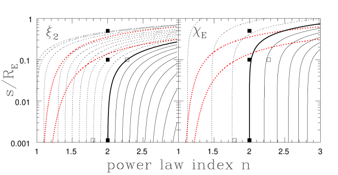
Figure 1: The parameter space of the softened power law models. The left panel shows contours of $\xi_{2}$ with $\xi_{2}=0$ for the heavy solid curve and increasing (decreasing) in steps of $0.2$ for the solid (dashed) contours. The right panel shows contours of $\chi_{E}$ with $\chi_{E}=1/3$ for the heavy solid curve and increasing (decreasing) in steps of $0.1$ for the solid (dashed) contours. Above the upper (lower) red dotted curves, the central magnification exceeds $1$ ($0.1$). The solid (open) squares show some of the input (matched in $\xi_{2}$) models considered in the later sections. The singular models with $n=0$, $n=2$ and $n=3$ correspond to a constant surface density, an SIS and a point mass, respectively.

Shallow power-law density profiles, power-law models with finite cores, Hernquist (1990) and NFW (Navarro et al. 1997) profiles all produce unobserved central, “odd” images. Like Millon et al. (2019) we will simply ignore their existence in making the model comparisons. Fig. 1 shows where the softened power law models produce central magnifications $>0.1$ and $>1.0$ as a function of $n$ and $s/R_{E}$. The Millon et al. (2019) model with $n=2$ and $s=0.5R_{E}$ is somewhat perverse because the central image is actually magnified rather than demagnified. We will include a model with $n=2$ and $s=0.1R_{E}$ that is more reasonable (central $M<0.1$), although it would still produce a visible central image in many lenses.

The key point in Kochanek (2020) is that the only property of the radial mass distribution strongly constrained by lens data is

$$\xi_{2}={R_{E}\alpha^{\prime\prime}(R_{E})\over 1-\kappa_{E}}$$ (3)

where $R_{E}$ is the Einstein radius, $\kappa_{E}$ is the convergence and $\alpha^{\prime\prime}(R_{E})$ is the second derivative of the deflection profile both measured at the Einstein radius. This simply comes from carrying out a Taylor expansion of the lens equations and extracting the first term in the monopole beyond the Einstein radius that can be constrained by lens data and expressing it in a form which is invariant under the mass sheet degeneracy. We have added the subscript $2$ to indicate that it is the second order term in the expansion. This point is independent of any angular structure in the lens.

It is a Taylor expansion, so data can in theory constrain higher order terms in the structure of the monopole. The next dimensionless, mass-sheet invariant term would be $\xi_{3}=R_{E}^{2}\alpha^{\prime\prime\prime}(R_{E})/(1-\kappa_{e})$. For an Einstein radius of $R_{E}=1\aas@@fstack{\prime\prime}0$ and data in an annulus $|r-R_{E}|/R_{E}=30\%$ around $R_{E}$, the magnitude of the deflections created by $\xi_{2}$ are $\sim\xi_{2}|r-R_{E}|^{2}/2R_{E}\simeq 0\aas@@fstack{\prime\prime}045\xi_{2}$ which is relatively easy to constrain given the $0\aas@@fstack{\prime\prime}1$ resolution of the Hubble Space Telescope (HST). The scale of the deflections created by $\xi_{3}$ are of order $\xi_{3}|r-R_{E}|^{3}/6R_{E}^{2}\simeq 0\aas@@fstack{\prime\prime}0045\xi_{3}$, which will be difficult to constrain given both the resolution of the data and the many systematic issues that begin to enter on these scales (PSF models, pixelization, lens galaxy contamination, millilensing, etc.). To make this a little more concrete, simply consider the power law models where $H_{0}\propto 1-\kappa_{E}=(2+\xi_{2})/4$. For $\kappa_{E}\simeq 0.5$, a 2% uncertainty in $H_{0}$ requires a $\Delta\xi_{2}\simeq 1\%$ uncertainty in $\xi_{2}$, which corresponds to deflection differences between the models across the annulus of order $\Delta\xi_{2}|r-R_{E}|^{2}/2R_{E}\simeq 0\aas@@fstack{\prime\prime}00045$! And this is for a model which, unlike realistic models, has a one-to-one relation between $\kappa_{E}$ and $\xi_{2}$.

For a power law model, $\xi_{2}=2(n-2)$, so it is zero for the $n=2$ SIS. There is a general analytic expression for $\xi_{2}$ in the power law models, but it is too long to be worth reporting. Fig. 1 shows contours of $\xi_{2}$ in the $n$ and $s/R_{E}$ plane. For singular models, $n=1$ is a constant density sheet, $n=2$ is the SIS, and $n=3$ is a point mass. For sufficiently small cores, $\xi_{2}$ converges to the power law limit. Its value decreases with increasing core radius at fixed exponent $n$ and increases with increasing $n$ at fixed core radius $s/R_{E}$. Solid points mark three of the input models we will consider ($n=2$, $s/R_{E}=0$, $0.1$ and $0.5$). Open points mark the $s/R_{E}=0.1$ and $s/R_{E}=0$ models that match the values of $\xi_{2}$ for the first two cases. Matching the $\xi_{2}$ value of the $n=0$, $s/R_{E}=0.5$ model requires power-law profile with $n<1$, which means that the surface density is increasing with radius and the corresponding open point lies off the figure to the left. As we will see in §3, even with large numbers of constraints spread across a fairly broad annulus, circular lens models have tremendous difficulty distinguishing these $\xi_{2}$-matched models.

The simplest way to think about angular structure is in terms of multipoles (see Kochanek 2006). For pedagogic purposes we will consider only ellipsoids and shears (anti)aligned with the coordinate axes, although any result can be generalized. We consider a density distribution $\kappa(\xi)$ with $\xi^{2}=x^{2}+y^{2}/q^{2}$ and $\epsilon=1-q$. For simple analytic results, we will assume $\epsilon$ is small and expand results only to their lowest order in $\epsilon$. If we just keep the lowest order monopole and quadrupole terms, the monopole density is

$$\kappa_{0}(r)={1\over 2\pi}\int_{0}^{2\pi}d\theta\kappa(\xi)\simeq\kappa(r)$$ (4)

and the quadrupole density is

$$\kappa_{2}(r)={1\over\pi}\int_{0}^{2\pi}d\theta\cos(2\theta)\kappa(\xi)\simeq-\epsilon rk^{\prime}(r)/2.$$ (5)

where the limiting cases assume $\epsilon$ is small. The combined density is $\kappa(r,\theta)=\kappa_{0}(r)+\kappa_{2}(r)\cos 2\theta$ which corresponds to a lensing potential of $\Psi(r,\theta)=\Psi_{0}(r)+\Psi_{2}(r)\cos 2\theta$ where the monopole potential is

$$\Psi_{0}=2\log(r)\int_{0}^{r}du\kappa_{0}(u)u+2\int_{r}^{\infty}du\kappa_{0}(u)u\ln u.$$ (6)

We can write the quadrupole potential as

$$\Psi_{2}=-{1\over 2}r^{2}\gamma(r)-{1\over 2}r^{2}\Gamma(r)$$ (7)

where

$$\gamma(r)=\int_{r}^{\infty}du\kappa_{2}(u)/u$$ (8)

is the contribution from outside radius $r$ (i.e., like an external shear) and

$$\Gamma(r)={1\over r^{4}}\int_{0}^{r}duu^{3}\kappa_{2}(u)$$ (9)

is the contribution from the material inside radius $r$ (the “internal” shear). Like an external shear, both $\gamma(r)$ and $\Gamma(r)$ are dimensionless. The deflections due to the quadrupole are then

$$\vec{\alpha}_{2}=-r\gamma(r)\left[\begin{array}[]{r}\cos\theta\\ -\sin\theta\end{array}\right]-r\Gamma(r)\left[\begin{array}[]{r}\cos 3\theta\\ \sin 3\theta\end{array}\right].$$ (10)

If we decompose the deflections into the radial deflections

$$\hat{e}_{r}\cdot\vec{\alpha}_{2}=-r\left[\gamma(r)+\Gamma(r)\right]\cos 2\theta$$ (11)

and the tangential deflections

$$\hat{e}_{\theta}\cdot\vec{\alpha}_{2}=r\left[\gamma(r)-\Gamma(r)\right]\sin 2\theta$$ (12)

we can see that to (lowest order), a model must have two angular degrees of freedom in order to fit an Einstein ring, the internal shear $\Gamma_{E}$ and the external shear $\gamma_{E}$ at the Einstein ring. Alternatively, the overall ellipticity of the ring is set by $\gamma_{E}+\Gamma_{E}$ while the detailed shape depends on $\chi_{E}=\Gamma_{E}/\gamma_{E}$. Time delays also depend on having the correct value of $\chi_{E}$ (see Kochanek 2006). Like the monopole, there are then higher order, sub-dominant terms (gradients of the quadrupole at the ring, deviations of the octopole from the predictions of whatever model is producing the quadrupole and so forth) even before considering the additional degrees of freedom associated with variable axis orientations.

An ellipsoidal model has, however, only one angular degree of freedom, the axis ratio $q=1-\epsilon$. Once the axis ratio is chosen, the ratio $\chi_{E}=\Gamma_{E}/\gamma_{E}$ is fixed, so an ellipsoidal model will only be able to fit Einstein rings produced by models with the same $\chi_{E}$. At least for the low ellipticities used in the numerical models we consider later in the paper, $\chi_{E}$ is independent of the actual value of $\epsilon$. For higher ellipticities, there would be non-linear corrections in $\epsilon$ to the ratio $\chi_{E}$.

The right panel of Fig. 1 shows contours of $\chi_{E}$ for the softened power-law models. The singular models have $\chi_{E}=(n-1)/(5-n)$, so the $n=2$ SIS has $\chi_{E}=1/3$. Like $\xi_{2}$, the general expression for $\chi_{E}$ is analytic but too long to be worth presenting. Although the general morphology of the $\chi_{E}$ and $\xi_{2}$ contours are similar, they do not track one another in detail. Hence, the $\chi_{E}$ values of the models matched in $\xi_{2}$ (the open and closed point pairs) lie on different $\chi_{E}$ contours. A model at an open point will fail to provide a good fit to the angular structure of an Einstein ring produced by a model at the associated closed point.

This inability to simultaneously match $\xi_{2}$ and $\chi_{E}$ is the reason that Millon et al. (2019) find such large likelihood differences between mass models, not that Einstein rings have any great ability to constrain radial mass distributions. In §3 we demonstrate that even large numbers of constraints in a fairly thick annulus around $R_{E}$ determine $\xi_{2}$ and basically nothing else. In §4 we reproduce the large likelihood differences found by Millon et al. (2019) when trying to model an Einstein ring produced by one ellipsoidal model with an ellipsoid having a different radial mass profile.

However, no realistic lens model consists only of a single ellipsoid. A barely realistic model includes an external shear $\gamma_{0}$, in which case $\chi_{E}=\Gamma_{E}/(\gamma_{E}+\gamma_{0})$ for an (anti)aligned external shear. By appropriately adjusting the external shear, the $\xi_{2}$ and $\chi_{E}$ values of the input and output models can be matched simultaneously. Thus, we predict, and find in §4, that adding this generically required extra parameter to the angular structure makes the huge likelihood differences between models found by Millon et al. (2019) simply vanish.

3 Constraining the Radial Mass Distribution

In this section we consider only circular lenses and so simply solve the one-dimensional lens equations in a stand alone program. In all the models, we make the Einstein radius $R_{E}\equiv 1$. We set the ratios of the other scales (like $s$) to closely match the dimensionless scale ratios of Millon et al. (2019), although as relatively round numbers. For each test, we generate the images for either 4 or 50 multiply imaged sources and then model them without adding any noise.

We fit only the image positions, scaling the goodness of fit statistic $\chi^{2}$ assuming astrometric errors of $\sigma=0.004R_{E}$. For $R_{E}=1\aas@@fstack{\prime\prime}0$, this uncertainty of 0$\aas@@fstack{\prime\prime}$004 is 10% of an HST WFC3/UVIS or ACS pixel and 3% of a WFC3/IR pixel. The positions of the point-like quasar images can be measured somewhat better, although in the CfA-Arizona Space Telescope Lens Survey (CASTLES, e.g., Lehár et al. 2000) we generally limited our astrometric uncertainties to about this scale ($0\aas@@fstack{\prime\prime}003$) due to systematic differences from different PSF models, extended emission, pixelization and millilensing. The effective astrometric accuracy associated with the extended emission of an Einstein ring, which is what we are mimicking using large numbers of multiply imaged sources, will be lower because the emission is smooth. In any case, the changes in likelihood between models will be representative of any error model. Because we added no noise, a fit using the input model yields $\chi_{in}^{2}=0$, so the likelihood ratio between the input model and a fit with an alternative model leading to a fit statistic $\chi^{2}$ is simply $\exp(-\chi^{2}/2)$.

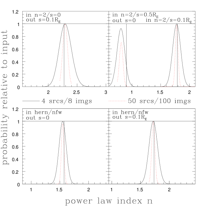
Figure 2: Likelihood ratios relative to the true model as a function of the power law exponent $n$ for either 4 lensed sources (black solid) or 50 lensed sources (red dashed). The vertical line indicates the value of $n$ predicted by matching the values of $\xi_{2}$. The top left panel is for a $n=2$ singular isothermal sphere modeled by a cored power law with $s=0.1R_{E}$. The top right panel is for either a $n=2$, $s=0.5R_{E}$ or a $n=2$, $s=0.1R_{E}$ cored power law modeled by a singular power law. The lower panels are for a Hernquist plus NFW lens modeled by either a singular (left) or $s=0.1R_{E}$ cored power law (right).

For the four source case, we placed the outer images of each image pair at $r_{out}=1.01$, $1.1$, $1.2$ and $1.3R_{E}$. and then solve for the position of the inner image to produce fake image data. For the fifty source case, we randomly selected radii for the outer image as $r=R_{E}(1+0.3P^{1/2})$, which roughly corresponds to uniformly sampling a disk centered behind the lens. In all of these models we fix the position of the lens galaxy to its true position. Allowing the position of the lens galaxy to shift will lead to a further reduction in the ability to differentiate models, but it will be a small correction for models with a large number of sources and images.

The first two cases considered by Millon et al. (2019) model a lens produced by a singular isothermal sphere (SIS, $n=2$, $s=0$) with the general power law lens. As noted earlier, the singular models have $\xi_{2}=2(n-2)$, so this input model has $\xi_{2}=0$. As a function of $n$ we can determine the core radius $s$ needed to have $\xi_{2}=0$, finding that there are no solutions for $n<2$, and that the necessary core radius then increases with $n$, starting from $s=0$ at $n=2$. So, for example, a lens with $n=2.274$ and $s=0.1R_{E}$ should be virtually indistinguishable from the input model (see Fig. 1).

The results for fitting a $n=2$, $s=0$ model with $s=0.1R_{E}$ models are shown in the upper left panel of Fig. 2. The cored model fits either case almost perfectly, and almost exactly at the power law index predicted to match the values of $\xi_{2}$. The two models would, however, yield significantly different estimates of $H_{0}$ since the singular $n=2$ model has $\kappa_{E}=1/2$ while the cored model has $\kappa_{E}=0.44$, Note, however, that the inability to distinguish the two models is due neither to using a narrow annulus (the width is 60% of $R_{E}$) nor due to having few constraints (there are 50 image pairs).

The second set of models considered by Millon et al. (2019) generate a lens with a $n=2$ cored power law and then fit it using a singular model. In round numbers, the input model has $n=2$ and $s=0.5R_{E}$. As noted earlier, this is a somewhat pathological model due to the large core. Its power-law match at $\xi_{2}=-2.189$ has $n=0.906$, which is also somewhat pathological because the model has a radially increasing surface density. Because of the large radial critical curve of the input model, we had to move the outermost image radius from $1.3R_{E}$ to $1.25R_{E}$ to keep all the sources multiply imaged. Nonetheless, we can still check the mathematical statement that the models should be virtually indistinguishable. As we see in the upper right panel of Fig. 2, the match is not quite as good as in the first example. The model is somewhat offset from the value of $n$ predicted by matching the values of $\xi_{2}$ and the likelihood ratios are modestly different from unity. Still, even with 50 multiply imaged sources, the likelihood ratio is $0.7$, which is not very significant.

As a more realistic version of this test, we used $n=2$ and $s=0.1R_{E}$ for the input model, which now has a demagnified central image and allows us to move the outermost images back to $1.3R_{E}$. As shown in Fig. 1 the predicted power law match in $\xi_{2}$ has $n=1.791$, and this model provides an essentially perfect fit whether we use four or fifty multiply imaged sources, as also shown in the upper left panel of Fig. 2.

The final set of models considered by Millon et al. (2019) combine a Hernquist (1990) and a NFW (Navarro et al. 1997) profile to generate the lens. To match their first such model, we used a Hernquist scale length of $s=1.5R_{E}$, an NFW scale length of $a=30R_{E}$ and normalize the models to have $\kappa=3$ at $r=0.1R_{E}$ so that the density profile closely matches that in Millon et al. (2019). The resulting model has $\xi_{2}=-0.852$ which corresponds to $n=1.574$ for a pure power law model and $n=1.734$ for a power law model with a $s=0.1R_{E}$ core radius. As shown in the lower panels of Fig. 2, the models matched in $\xi_{2}$ again provide near perfect fits for both 4 and 50 multiply imaged sources. The last model considered by Millon et al. (2019) chooses parameters for the Hernquist and NFW profiles to produce a density distribution that very closely mimics the singular $n=2$ power law model, so there is nothing new to be tested in this case.

Not surprisingly, mathematics works, and it is very difficult to distinguish radial mass distributions matched in $\xi_{2}$ even with very large numbers of lensed images assumed to have very well-measured positions. With even a little more freedom in the radial mass distribution, the small remaining likelihood differences would be relatively easy to eliminate. In short, multiple lensed sources and Einstein rings basically constrain nothing about the radial mass distributions other than $R_{E}$ and $\xi_{2}$.

4 How the Angular Tail Wags the Radial Dog

Millon et al. (2019) argue that the reason they can distinguish radial mass distributions is because of the large numbers of constraints supplied by the Einstein ring images of the hosts. As we demonstrated in the previous section, even large numbers of radial constraints spanning a fairly broad annulus around the Einstein radius cannot distinguish radial mass distributions with the same value of $\xi_{2}$. Einstein rings do, however, provide a huge number of constraints on the angular structure of the gravity. This can be seen both in the theory of Einstein ring formation (Kochanek et al. 2001) and in the ability of the rings to constrain deviations in the gravity from ellipsoidal (e.g., Yoo et al. 2005, Yoo et al. 2006). The Millon et al. (2019) simulations assumed ellipsoidal models with no external shear, so they had very limited degrees of freedom in the angular structure of the gravity.

For each input mass distribution, we first model it as an ellipsoid without any external shear, and then as an ellipsoid plus an (anti)aligned external shear. We show the results for both 4 and 50 multiply imaged sources to illustrate the consequences of adding more and more constraints on the angular structure for the inferred likelihood ratios of the radial structures. Then at the end of the section we consider models with more complex angular structures like the misaligned Hernquist (1990) plus NFW (Navarro et al. 1997) models in Millon et al. (2019).

Figure 3: The distribution of the 104 lensed images used for the $n=2$, $s=0$ ellipsoidal input model. There are two sets of four images (filled squares), 48 sets of two images (open triangles) and $104$ images in total. The curve shows the location of the tangential critical line, and this singular lens has no radial critical line. The sources used to generate the images were randomly distributed over a disk of radius $0.3R_{E}$ on the source plane. The cross in the lower left corner is ten times larger than the assumed astrometric errors of $0.004R_{E}$.

For the numerical models in this section we use lensmodel (Keeton 2001, Keeton 2011) to generate and fit the test cases. For the four source case we place sources at radii of $0$, $0.1$, $0.2$ and $0.3R_{E}$ on the source plane and at a random angle. For the 50 source case we randomly distributed the sources uniformly over a source plane region of radius $0.3R_{E}$. The angular positions are chosen randomly. The Millon et al. (2019) models all have axis ratios of $q\simeq 0.9$, so we simply set $q=0.9$. These models are nearly circular, so they produce very few four image systems. The four image cross section of an elliptical lens is of order $(\epsilon R_{E}/3)^{2}$ where $q=1-\epsilon$ and $\epsilon/3$ is roughly the ellipticity of the potential, so only $\sim 1\%$ of the region inside a source radius of $0.3R_{E}$ will produce four images. Fig. 3 shows the 104 images from 50 multiply imaged sources (i.e., two sources produced four images, the rest two images) for the first input case we consider with $n=2$ and $s=0$. The symbols used in the plot are roughly ten times larger than the assumed astrometric uncertainties of $0.004R_{E}$.

For the basic models we use a single axis ratio for the input models and align the models with the coordinate axes. We then model the system holding the lens position fixed and forcing the model ellipsoid and shear to be (anti)aligned with the same axes. The fits would improve if these were allowed to vary. In their input Hernquist (1990) plus NFW (Navarro et al. (1997) models, Millon et al. (2019) allow them to have slightly different axis ratios and to be slightly misaligned. Obviously, a single ellipsoid fit to such a model has too few degrees of freedom in its angular structure, so we will return to allowing these extra degrees of freedom in the input model after first considering the simple case where the two profiles are aligned and have the same ellipticity.

We do not include the $n=2$, $s=0.5R_{E}$ input model in this section, as lensmodel has difficulty finding solutions for the matched $n\simeq 0.9$ power-law with a radially increasing surface density. The difficulties probably arise because this model is so close to the degenerate $n=1$ constant surface density model and it is a regime where there was no physical need to ever make lensmodel work reliably. We could compute a goodnesses of fit using lensmodel’s “source plane” fit statistic (which is really the position mismatch on the source plane locally corrected for image magnifications), but not for the true “lens plane” fit statistic. The qualitative results for the “source plane” fit statistic agree with those for the other cases but the quantitative reliability of the results is unclear. Since both the input and output models are unrealistic, we study only the $n=2$, $s=0.1R_{E}$ case we introduced in §3.

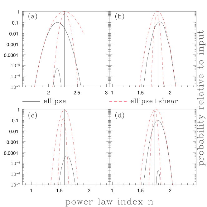
Figure 4: Likelihood ratios relative to the true ellipsoidal model as a function of the power law exponent $n$ for either a purely ellipsoidal model (black solid) or an ellipsoid plus an (anti)aligned shear (red dashed). The top left panel (a) is for a $n=2$ SIS sphere modeled by a cored power law with $s=0.1R_{E}$. The top right panel (b) is for a $n=2$, $s=0.1R_{E}$ cored power law modeled by a singular power law. The lower panels are for a Hernquist plus NFW lens modeled by either a singular (left, (c)) or $s=0.1R_{E}$ cored power law (right (d)). In each case, the higher likelihood ratio model has 4 multiply imaged sources and the lower likelihood one has 50. In some cases, the 50 source purely ellipsoidal model has a peak likelihood too low to appear.

We start with the input SIS ($n=2$, $s=0$) input model, where the images for the 50 source realization are shown in Fig. 3. As shown in Fig. 1, the $s=0.1R_{E}$ model matched in $\xi_{2}=0$ has $n=2.274$, but this model differs in its angular structure $\chi_{E}$ from the input model. The top left panel of Fig. 4 shows the results. With four multiply imaged sources, the log likelihood ratio relative to the input model for four sources is $\sim-1.0$ dex, while for 50 sources it is $\sim-5.3$ dex, which Millon et al. (2019) interpret as successfully distinguishing between the radial mass distributions. The best models are also shifted away from the value of $n$ which would match the input value of $\xi_{2}$ towards the $n$ of the input model. This allows the model to come closer to the angular structure of the input model. However, if we now add an (anti)aligned shear, the log likelihood ratios become $-0.03$ and $-0.22$ dex, respectively, and the models are practically indistinguishable ($-0.22$ dex corresponds to $\Delta\chi^{2}=1$). The best value of $n$ is also now centered on the value predicted from matching the values of $\xi_{2}$.

The top right panel of Fig. 4 shows the results for modeling the $n=2$, $s=0.1R_{E}$ softened power law model with a singular power law. For the purely ellipsoidal model, the log likelihood ratios are $-1.0$ and $-7.4$ dex, respectively, where the likelihood curve for the 50 source case does not even appear in the figure despite the dynamic range. However, with the addition of the anti(aligned) shear, the likelihood ratios drop to $-0.03$ and $-0.3$ dex, again making the models practically indistinguishable.

Finally, Fig. 4 shows the results for the Hernquist (1990) plus NFW (Navarro et al. 1997) input models, where for a first test we gave the two profiles the same $q=0.9$ axis ratio and the same major axis position angle. If we first consider the singular models without any external shear, the likelihood ratios are enormous at $-4.3$ and $-20.1$ dex for four and 50 multiply imaged sources, respectively. When we add a (anti-)aligned shear, the likelihood ratios drop to $-0.1$ and $-0.8$ dex, respectively. Similarly, the $s=0.1R_{E}$ models have poor fits as only ellipsoids (likelihood ratios of $-1.0$ and $-5.7$ dex) and quite good fits as ellipsoids plus an external shear (likelihood ratios of $-0.0$ and $-0.2$ dex).

In practice, the combined Hernquist (1990) and NFW (Navarro et al. 1997) models used by Millon et al. (2019) used slightly different major axis position angles ($\Delta PA=2.1^{\circ}$ for their model #5) for the two components. It is unclear why adding additional angular structure and then fitting a single ellipsoid was viewed as a test of recovering the radial mass distribution. As an additional experiment we generated a similar model, using $q=0.9$ for both components and an axis shift of $\Delta PA=2^{\circ}$ and then fit it with both the $s=0$ and $s=0.1R_{E}$ power law models allowing the orientations of both the ellipsoid and the shear to vary. Considering only the 50 source models, the best fit ellipsoid with $s=0$ ($s=0.1R_{E}$) had a likelihood ratio of $-0.80$ dex at $n=1.45$ ($-0.19$ dex at $n=1.26$), which is surprisingly good given that the model simply cannot fully reproduce the angular structure of the input model. Nonetheless, the additional angular structure from having two misaligned model components worsens the fits compared to the models where the two components were kept aligned. This increases the apparent likelihood difference between the radial mass distributions, but it is a again false inference created by the assumed angular structures rather than an ability to discriminate the radial mass distributions.

5 Discussion

It is true, as Millon et al. (2019) argue, that Einstein ring images of host galaxies (or equivalently large numbers of multiply imaged sources as we use here) provide a large number of constraints on a lens model. It is, however, exceedingly dangerous to impose large numbers of constraints on lens models with insufficient degrees of freedom. This has been discussed many times in the context of the radial mass distribution (Gorenstein et al. 1988, Kochanek 2002, Kochanek 2006, Schneider, & Sluse 2013, Wertz et al. 2018, Sonnenfeld 2018, Kochanek 2020). As we demonstrate in §2, Einstein rings are not very good at discriminating between radial mass distributions – they will simply identify models with the same $\xi_{2}$ and little else, as we argued in Kochanek (2020).

Einstein rings are, however, exceedingly good at determining the angular structure of the gravitational potential (Kochanek et al. 2001, Yoo et al. 2005, Yoo et al. 2006). If there are insufficient degrees of freedom in the allowed angular structure of the models, this will drive the selection of the radial mass distribution and may still lead to a poor fit. In their models to rebut Kochanek (2020), Millon et al. (2019) find enormous likelihood ratios between the models and interpret this as being able to distinguish the radial mass distributions. However, as we show in §2, the results were entirely driven by restricting the mass models to be ellipsoids without an external shear. When we take the same models and include an external shear, the likelihood differences nearly vanish, and there is essentially no ability to distinguish the radial mass distributions even when using 50 multiply imaged sources with positions measured to $0\aas@@fstack{\prime\prime}004$ for an Einstein radius of $R_{E}=1\aas@@fstack{\prime\prime}0$. By adding a few additional degrees of freedom to either the radial or angular structure of the mass model, one could reduce the rather statistically insignificant residual differences still further.

The only way to be certain that the angular information is not driving an apparent ability to discriminate between radial mass distributions (and hence the value of $H_{0}$) is to ensure that the angular structure has all the physical degrees of freedom of real galaxies. All models of real lens systems include external shears, one reason that the actual H0LiCOW (e.g., Wong et al. 2019) lens models do not find likelihood ratios between monopole models nearly as large as in Millon et al. (2019). However, even an ellipsoid plus an external shear clearly has too few degrees of freedom to have any confidence that a statistical difference between two models for the monopole is being driven by an actual ability to distinguish the monopoles, rather than it being an illusory distinction driven by assumptions in the angular structure.

Physically, we know galaxies are minimally comprised of both a stellar component and a dark matter component and that these will have different ellipticities and can be modestly misaligned. But it is much more complex than that, because we also know that they can show ellipticity gradients, axis twists, and deviations from ellipsoidal isodensity contours (e.g., “boxy” or “disky” isophotes). All of these complications steadily decouple the angular structure of the gravity from the monopole of the gravity. Suppose, for example, that we consider a one parameter series of monopoles, like the power law models and generate a lens with $n=2$ but with an ellipticity that increased with radius. If we model this lens with a simple ellipsoid, the strong constraints of an Einstein ring will disfavor $n=2$ because it is producing too little exterior shear as compared to interior shear. The models will be driven to a shallower radial mass profile (smaller $n$) because, with more mass outside the Einstein ring, the model can increase the exterior shear relative to the interior shear. This of course then produces a bias on any estimate of $H_{0}$.

In short, without models that include many more angular degrees of freedom, it would be best to simply not include the constraints from Einstein rings. It is also another reason that the power law models should simply be abandoned. Not only do they have a one-to-one mapping between $\xi_{2}$ and $\kappa_{E}$ that will systematically underestimate the uncertainties in the convergence at the Einstein radius (and $H_{0}$), but they also have a far too little freedom in their angular structure, particularly if you are fitting Einstein rings. Even if you had some legitimate basis (which you do not) to ignore ellipticity gradients, axis twists and deviations from ellipsoidal isodensity contours, you still have a stellar mass distribution and a dark matter distribution which are essentially guaranteed to have different ellipticities and even this most basic property of real galaxies cannot be captured by the power-law models. The lack of an independent parameter for the difference in ellipticity on small (stars) and large (dark matter) scales, is essentially another “knob” like the shear we considered here. But it is more general because when combined with the freedom from the external shear, it provides more degrees of freedom for higher order effects like the gradients in the angular structure at the Einstein ring and the ability to adjust the higher order multipoles that can modify the structure of Einstein rings while keeping the quadrupole structure fixed.

The statistical approach used by Millon et al. (2019) also has a problem in that it penalizes models for including degrees of freedom which must be present in real galaxies. Millon et al. (2019) use the Bayesian Information Criterion (BIC),

$$BIC=k\ln n-2\ln L$$ (13)

where $L$ is the model likelihood, $k$ is the number of parameters and $n$ is the number of constraints. The BIC heavily penalizes the introduction of new parameters when there are large numbers of constraints $n$, as is true of Einstein ring images. For example, the alternative Akaike Information Criteria,

$$AIC=2k-2\ln L$$ (14)

penalizes the addition of new parameters far less than the BIC. Viewed as a change in a $\chi^{2}$ statistic ($\ln L=-\chi^{2}/2$), AIC views the introduction of a new parameter as neutral if $\Delta\chi^{2}=1$, while BIC views it as neutral if $\Delta\chi^{2}=(1/2)\ln n$. Philosophically, AIC should be preferred over BIC for problems like determining $H_{0}$ where it is important to avoid obtaining a precise but potentially inaccurate result.

More deeply, however, the information criteria should only be applied to the introduction of new parameters for which there is a plausible physical reason that the parameter values are known a priori and so holding them fixed is a reasonable prior. But this simply is not true for any aspect of standard lens models – our a priori knowledge is that the standard models are too simple and require additional parameters if they are to be realistic models of the actual mass distributions of galaxies. The more complex models are intrinsically more probable, not less probable, than the simple models, exactly the opposite of the assumptions of the information criteria. The proper way to treat these complexities is to include all the degrees of freedom of real galaxies but with priors on their values (e.g., ellipticity gradients are not zero, but they are small, etc.). For Einstein rings, the same issues hold for models of the source galaxy if they are parametrized analytic models rather than pixellated source models. Quasar host galaxies are no more likely to be perfect ellipsoids than lens galaxies.

Finally, as noted in Kochanek (2020), the H0LiCOW (e.g., Wong et al. 2019) models show too little sensitivity to the available stellar dynamical constraints compared to expectations, and Millon et al. (2019) document this lack of sensitivity extensively. The lack of sensitivity to the dynamical data is not a positive aspect of the existing models – it is a clear proof that the mass models have too few degrees of freedom. The lens data so tightly constrain $R_{E}$ and $\xi_{2}$ that the dynamical information is effectively ignored because of its larger fractional uncertainties. This is unfortunate, because, unlike Einstein rings, dynamical data actually does help to constrain $\kappa_{E}$. At least for the radial mass distribution, one would actually have more reliable constraints on $\kappa_{E}$ by simply ignoring the Einstein ring and relying on the dynamical data. A simple test for whether mass models have sufficient degrees of freedom is that the they should show the expected sensitivity to the dynamical data, namely that the fractional uncertainties in $H_{0}$ should be comparable to the fractional uncertainties in the velocity dispersion (see Kochanek 2020).

References

- Auger et al. (2010) Auger, M. W., Treu, T., Bolton, A. S., et al. 2010, ApJ, 724, 511
- Bolton et al. (2012) Bolton, A. S., Brownstein, J. R., Kochanek, C. S., et al. 2012, ApJ, 757, 82
- Gavazzi et al. (2007) Gavazzi, R., Treu, T., Rhodes, J. D., et al. 2007, ApJ, 667, 176
- Gorenstein et al. (1988) Gorenstein, M. V., Falco, E. E., & Shapiro, I. I. 1988, ApJ, 327, 693
- Hernquist (1990) Hernquist, L. 1990, ApJ, 356, 359
- Keeton (2001) Keeton, C. R. 2001, arXiv e-prints, astro-ph/0102340
- Keeton (2011) Keeton, C. R. 2011, GRAVLENS: Computational Methods for Gravitational Lensing, ascl:1102.003
- Kochanek et al. (2001) Kochanek, C. S., Keeton, C. R., & McLeod, B. A. 2001, ApJ, 547, 50
- Kochanek (2002) Kochanek, C. S. 2002, ApJ, 578, 25
- Kochanek (2006) Kochanek, C. S. 2006, Saas-fee Advanced Course 33: Gravitational Lensing: Strong, Weak and Micro, 91
- Kochanek (2020) Kochanek, C. S. 2020, MNRAS, 493, 1725
- Koopmans et al. (2009) Koopmans, L. V. E., Bolton, A., Treu, T., et al. 2009, ApJL, 703, L51
- Lehár et al. (2000) Lehár, J., Falco, E. E., Kochanek, C. S., et al. 2000, ApJ, 536, 584
- Millon et al. (2019) Millon, M., Galan, A., Courbin, F., et al. 2019, arXiv e-prints, arXiv:1912.08027
- Navarro et al. (1997) Navarro, J. F., Frenk, C. S., & White, S. D. M. 1997, ApJ, 490, 493
- Rusin, & Kochanek (2005) Rusin, D., & Kochanek, C. S. 2005, ApJ, 623, 666
- Schneider, & Sluse (2013) Schneider, P., & Sluse, D. 2013, AAP, 559, A37
- Sonnenfeld (2018) Sonnenfeld, A. 2018, MNRAS, 474, 4648
- Wertz et al. (2018) Wertz, O., Orthen, B., & Schneider, P. 2018, AAP, 617, A140
- Wong et al. (2019) Wong, K. C., Suyu, S. H., Chen, G. C.-F., et al. 2019, arXiv e-prints, arXiv:1907.04869
- Yoo et al. (2005) Yoo, J., Kochanek, C. S., Falco, E. E., et al. 2005, ApJ, 626, 51
- Yoo et al. (2006) Yoo, J., Kochanek, C. S., Falco, E. E., et al. 2006, ApJ, 642, 22