Towards Data Auctions with Externalities

Abstract

The design of data markets has gained importance as firms increasingly use machine learning models fueled by externally acquired training data. A key consideration is the externalities firms face when data, though inherently freely replicable, is allocated to competing firms. In this setting, we demonstrate that a data seller’s optimal revenue increases as firms can pay to prevent allocations to others. To do so, we first reduce the combinatorial problem of allocating and pricing multiple datasets to the auction of a single digital good by modeling utility for data through the increase in prediction accuracy it provides. We then derive welfare and revenue maximizing mechanisms, highlighting how the form of firms’ private information – whether the externalities one exerts on others is known, or vice-versa – affects the resulting structures. In all cases, under appropriate assumptions, the optimal allocation rule is a single threshold per firm, where either all data is allocated or none is.

Keywords:

Data Markets, Mechanism Design, Externalities

Declaration of interests:

None

1 Introduction

There are two key trends in the current era of statistical analysis: (i) an increase in the ease and scale of data collection and exchange due to the growing digitization of modern life; (ii) an increase in the richness of what one can learn from data via large scale statistical analysis due to improved computing capabilities. This is why more and more firms are deploying statistical models to improve their operations and make better decisions regarding, for example, what, when and how much to produce and at what price.

The key differentiating factor that determines the accuracy of these statistical models is access to high-quality data used to train these models, which we henceforth call training data. However, obtaining relevant training data can be challenging for firms to do themselves. This is especially true for firms that do not have the requisite data infrastructure setup to collect the data they need from their internal operations.

In light of the increased usefulness of training data and the growth of data services, firms are increasingly becoming sensitive to the negative externality they face when data is allocated to competing firms. Such a negative externality arises because firms that buy similar data often interact in a downstream market, and the use of data confers on a given firm a competitive advantage which hinders its competitors’ performance. For example, the data being sold could provide information about consumer preferences in the downstream market, which can help a firm capture a larger share of the market via product differentiation. Thus, although data is a freely replicable digital good and in principle can be sold to all firms interested in buying it, a data seller aiming to maximize revenue or welfare must consider the competition structure between buyers in deciding which firms to sell data to, how much to sell, and at what price. Notably, the formal literature which analyzes mechanisms to exchange training data between a collection of buyers and sellers is sparse. Thus, in this paper, we seek to provide a formal answer to the question:

How does the presence of externalities affect the optimal design of data markets?

This question can be approached by solving two coupled problems: First, can we define a tractable yet expressive model for how a buying firm values a collection of datasets, and for the externality such a firm experiences when a competing firm is allocated data? Second, given such a model, can we derive the optimal mechanism (e.g., in terms of revenue generated) to sell data, and how is such a mechanism affected by the presence of externalities? Below, we give an overview of how we tackle these two closely related problems and the answers they provide to the key question posed above.

How to Model a Buyer’s Valuation for Data?

The challenge of modeling a buyer’s utility for data stems from certain characteristics that are intrinsic to virtually all training data used to fit a statistical model: (i) datasets are freely replicable and so have no inherent scarcity; (ii) data is not fungible, and in fact its value is intrinsically combinatorial, i.e., different datasets (or different training features for a statistical model) are bound to have correlations in signal leading to sub-additive or super-additive valuations. In addition, in the presence of externalities, the value a buyer gets from a collection of datasets depends on the data allocated to other competing buyers. Thus a naive parameterization of a buyer’s valuation for a collection of datasets will be exponential in the number of datasets available and in the number of competing firms, rendering such a model intractable.

To circumvent these difficulties, we recall that a major motivation for firms to buy data is to make better predictions. Given this lens and building on the model in Agarwal et al. (2019), a key assumption we make in our formulation is that a buyer’s value for a collection of datasets comes directly from the increase in prediction accuracy it brings to a statistical model. Specifically, we assume that, for each buyer with a given prediction task, there is a commonly known function which maps each collection of datasets to a real number between $0$ and $1$. This number is a scalar summary of the increase in prediction accuracy of the statistical model – for example, this could be based on the (normalized) mean-squared error of a regression model trained using these datasets. A buyer’s value for a collection of datasets is then a non-decreasing function of this scalar summary of prediction accuracy. This formulation is not only crucial for a tractable model of a buyer’s valuation over datasets, but also, we believe, a better abstraction for reasoning about the value of data. The inferences drawn from a dataset, rather than the raw data itself, are what is of interest to the buyer of a dataset. Indeed, one would typically be willing to trade one dataset for another as long as the same inferences can be drawn from either of the two datasets.

Further, given that our aim is to understand the effect of externalities in a data market, our model needs to incorporate that a data buyer not only has a positive marginal value for acquiring data, but also has a negative marginal value for its competitors acquiring data. Thus a crucial extension to the model in Agarwal et al. (2019) is that we also assume that the prediction accuracy achieved by a given buyer induces a linear negative externality on each of the other buyers. This shift in perspective, from raw data to prediction accuracy, along with assuming a linear externality model reduces the combinatorial valuation of each buyer of data to $n$ parameters (where $n$ is the number of buyers): the positive marginal value for the buyer’s own prediction accuracy and the negative marginal values for the prediction accuracy of the remaining $(n-1)$ buyers.

The Design and Properties of a Data Market with Externalities.

Given the data valuation and externality model we introduce, we design a data auction for the setting of a monopolistic data seller and $n$ potential buyers (or bidders). Since we assume a buyer’s valuation for data is captured by the prediction accuracy, we show that the auction design problem reduces to one of selling a single divisible and freely replicable good. That is, instead of considering the seller as directly allocating data to buyers, we can equivalently consider the seller as allocating prediction accuracies resulting from the same data allocation. Still, a buyer’s bid is multidimensional since it includes private externality parameters in addition to a buyer’s marginal value for their prediction accuracy, and this multidimensionality makes characterizing the welfare-maximizing (i.e., efficient) and revenue-maximizing (i.e., optimal) mechanisms particularly challenging. Further, in such a market, two natural information structures are possible. In the first one, each buyer knows the externalities exerted on them by other buyers, i.e., the buyer’s negative marginal values for other buyers’ increases in prediction accuracy. In the latter the buyer knows the externalities that they exert on other buyers. We are thus tasked with describing different mechanisms corresponding to the specific information structure and objective being maximized (social welfare or revenue).

Optimal mechanism design with multidimensional bids is notoriously hard and our setting is no exception. When buyers privately know the externalities exerted on them by other buyers, we prove a reduction between the problem of auctioning multiple items to a single additive buyer and our setting. Understanding the structure of optimal mechanisms for the former problem is a major open question in auction theory (even for just two items and i.i.d. valuations). We thus make the problem tractable in this case by restricting either the mechanism structure, or the type distribution. In contrast, when buyers privately know the externalities they exert on other buyers, the problem simplifies and no such restriction is required: we show that the seller ignores the reported externalities and replaces them with their expected values under the common prior.

In all cases, the efficient and optimal mechanisms have a pleasantly simple structure: the allocation rules can be described by thresholds, resulting in allocations, to each given bidder, of either the entirety of the good (equivalently, all the data) or none of it. These thresholds balance a buyer’s marginal value for their own accuracy with others’ (negative) marginal values for the buyer’s accuracy. We also show that under appropriate assumptions, revenue maximization reduces to virtual surplus maximization: the optimal allocation is obtained by replacing the buyers’ marginal values with the corresponding virtual marginal values in the efficient allocation. This property was already observed in the context of single-item auctions (Myerson, 1981), hence our results extend it to the setting with externalities.

The thresholding structure of the optimal allocation has two important robustness implications: (i) the data seller does not require knowledge of the specific statistical models used by the buyers, nor of each buyer’s mapping from data to prediction accuracy, as long as the map is monotonic in the data allocated; (ii) if the prior distribution of private types is unknown, the optimal thresholds can be learned via an online optimization framework. We present such a framework in Appendix A for the case where the buyers’ bids are of the externalities they exert on others.

We now highlight some key properties of the optimal mechanisms that we derive, and how they are affected by externalities. First, we establish that in the presence of externalities, the maximum revenue a data seller can collect increases, even if the overall allocation decreases. This increase in revenue occurs as the data seller collects payments from firms to prevent allocations to other competing firms. Second, a perhaps counter-intuitive property of the optimal mechanisms is that the seller will in some cases collect a payment, which can also be viewed as an entry fee, even from buyers to whom nothing is allocated. This stems from the implicit threat induced by the allocation to other buyers resulting in a negative utility even when a buyer does not participate in the auction. Finally, the payment rules in the presence of externalities extend the intuition of standard second-price auctions. Here, bidders will be charged the minimum externality bid they would have needed to report in order to prevent another bidder from receiving an allocation, in addition to the minimum threshold they needed to bid in order to receive their own allocation. These key properties laid out above provide a meaningful answer to the main question of this paper posed earlier, of how externalities affect the optimal design of data markets.

As our key technical contribution, we extend the Myersonian auction format to the setting of a non-rival, excludable good with multidimensional bids that capture negative externalities. This provides novel results on the design and properties of the optimal mechanism for such settings.

Outline of the Paper.

We conclude the introduction with a discussion of the related work. In Section 2, we formulate the utility model of the firms, discuss our modeling assumptions and present the auction design problem. In Section 3 and Section 4 we describe the welfare- and revenue- maximizing mechanisms respectively. We conclude with a discussion of our main results in Section 5. In Appendix A, we extend our mechanism to when the prior distribution of types is unknown. The remaining appendices contain proofs of our results.

1.1 Related Work

Sale of Information Goods. A key aspect of the problems we consider is the fact that buyers of goods or information may interact downstream which affects their valuation of the overall allocation of the goods. Raith (1996); Ziv (1993) considered the related problem of sharing market-relevant information among competing oligopolists, and showed that the effect of such information sharing on the overall welfare of the firms depends on the type of competition in which they are engaged (e.g. Bertrand or Cournot competition), and the type of market-relevant parameters they are sharing (e.g. firms’ individual production cost estimates or a common market demand parameter). In some cases it is not optimal for any firm to share information with the others, due to the overwhelming negative effects of increased competition on their downstream profit. These findings motivate the study of how different forms of interdependent valuation functions may affect the welfare-maximizing or revenue-maximizing allocation of data.

More recently, there has been a range of works modeling the sale of information, usually some noisy signal of a market-relevant parameter, to a single data buyer Babaioff et al. (2012); Bergemann et al. (2018) or to competing firms Bimpikis et al. (2019); Admati and Pfleiderer (1988). Here, the information seller may add noise to the signal being sold, where such versioning is a unique feature of selling an information good, as well as restrict the set of firms who are offered the information. Similar to our results, both works find that under certain regimes of competition between firms, it is indeed optimal to sell to a strict subset of firms, balancing gains from information and negative externalities from competition. Bimpikis et al. (2019) shows specifically how the optimal selling strategy depends on downstream competition between the firms, but assumes that the competition structure and firms’ resulting utility functions are known to the information seller.

In reality, data buyers may have private informational priors and valuations on dataset allocations, which calls for the integration of an auction framework that incentivizes participation and truthful bidding by the buyers. A line of work studies mechanism design for the sale of data, in which the value of data is derived from its informativeness in a learning task. For procurement auctions, Ghosh and Roth (2011) consider a setting in which the buyer wishes to estimate a population statistic while the sellers experience a cost due to privacy loss. In Roth and Schoenebeck (2012), the authors consider a similar problem but assume a known prior on the sellers’ costs. A budget-feasible regression problem is considered in Horel et al. (2014) and Abernethy et al. (2015) consider an online learning setting. Agarwal et al. (2019) develops a two-sided market for selling and buying data, capturing the value of data through increases in prediction accuracy for buyer-specific machine learning models. In our work, we build on this model of valuation and study auctions of data in the presence of externalities.

Other recent works look specifically at the sale of consumer data to firms. Bergemann and Bonatti (2019) provide an excellent survey by considering a general data market framework featuring data buyers, data sellers, and data intermediaries. Key questions at hand include how data should be priced and possibly versioned, either directly by the data sellers or by the data intermediaries. Taylor and Wagman (2014) study specific settings in which firms in an oligopoly may use consumer data to set personalized prices, and find that the outcomes of data policies strongly depend on the oligopoly structure. Acemoglu et al. (2019) study a form of externalities between data sellers who value their privacy. In their model, correlations between consumer signals yield equilibria where consumers sell their data for very cheap prices despite having high values for privacy. Bergemann et al. (2020) similarly consider correlations between consumers’ data in the context of personalized pricing. The authors find that in order to maximize profits, a data intermediary should only sell an aggregate statistic, rather than individual values, of consumer demand to price-setting firms. Like Taylor and Wagman (2014), we consider externalities among data buyers, but assume a general model of additive negative externalities among the buyers that doesn’t necessarily have to arise from competition in oligopoly. Finally, Acquisti et al. (2016) provide a comprehensive review on the economic and privacy implications of collecting, using, and selling consumer data from both theoretical and empirical perspectives.

Auctions with Externalities.

Both efficient and optimal auctions of a single nondivisible good to multiple buyers are well understood in the absence of externalities among the buyers. A welfare-maximizing auction is given by the celebrated Vickrey auction (Vickrey, 1961) which is a second-price sealed bid auction, and a Bayesian-optimal auction for buyers with identical type distributions is given by a second-price auction with a reservation price (Myerson, 1981).

The most relevant line of work in the auction literature studies the question of designing auctions in the presence of externalities. The survey Jehiel and Moldovanu (2006) provides a useful reference. Optimal single-item auctions with additive allocative externalities among bidders were studied in Jehiel et al. (1996, 1999). They consider the same multidimensional, interdependent valuation setting as the one presented here, and provide characterizations of truthful and individually rational mechanisms. However, in order to solve revenue maximization under the information structure setting of known incoming externalities (defined in Section 2.4), Jehiel et al. (1999) impose restrictive symmetry assumptions which effectively reduce the problem to one with a single-dimensional bidding structure. In this paper, we provide a hardness result for the general revenue maximization problem and provide two additional conditions which each yield sensible, yet tractable solutions.

Many papers consider a similar additive model, but often assume that externality parameters are public Aseff and Chade (2008); Brocas (2013) or do not depend on the identity of the competitor Belloni et al. (2017), effectively reducing the auction to the single dimensional setting. Closest to our work is Deng and Pekec (2011) which extended the setting of Jehiel et al. (1996) to the situation where $K$ copies of the same indivisible item are being sold. However, their focus was on quantifying the effect of changing the parameter $K$. Finally, Haghpanah et al. (2013); Zhang et al. (2018) consider single-dimensional non-additive models of externalities yielding tractable auctions.

2 Model

We consider a single monopolistic data seller that has access to a (possibly combinatorial) data set, $S$ (e.g., $S$ could be a collection of $M$ training features). There are $n$ firms, in the set $N\coloneqq[n]$, which engage with this data seller to increase the prediction accuracy of some quantity of interest (e.g., forecasting demand of a good).

2.1 A Succinct Bidding Language for Data Auctions with Externalities

The key challenge in designing such data auctions stems from the potentially combinatorial nature of the data set $S$, on sale (e.g., $M$ training features). For example, the information in a particular feature is likely highly correlated with other features also sold by the data seller. Hence, without further structure, the number of parameters required to capture the valuation function of each firm (including the externalities due to other firms) is in general going to be exponential in the size of the data set $S$ and in the number of firms. For example in the case where there are $M$ features on sale, we would require at least $2^{n\cdot M}$ parameters to capture the valuation of each participating firm, likely rendering this auction intractable.

Towards Feasibility—Existence of a Prediction Gain Function.

Towards a more feasible auction design, we build on the model of Agarwal et al. (2019) and notice that in the setting where firms aim to increase prediction accuracy, it is natural to make the modeling assumption that their valuation for data does not come from specific data sets on sale, but rather from an increase in prediction accuracy of a quantity of interest (along with that of other firms when there are externalities). Hence, we assume that each firm $i\in N$ is parameterized by a “Gain Function”, $G_{i}:S\to[0,1]$, which is a function mapping the data set, $S$, to some quantity that defines prediction accuracy (e.g., (Normalized) Mean Squared Error, $R^{2}$-Accuracy). Implicit in $G_{i}$ are the particulars of the ML model that is trained and used to make predictions through the acquired information. As alluded to earlier, a different $G_{i}$ for each buyer indicates that we allow each buyer to have a different prediction task. Below we list two natural properties we impose on the gain function $G_{i}$ for each firm $i\in N$.

Property 1 (Monotonicity).

For any two subsets $S_{1}\subseteq S_{2}\subseteq S$, $G_{i}(S_{1})\leq G_{i}(S_{2})$.

Property 2 (Normalization).

We assume that $G_{i}$ is normalized such that $G_{i}(S)=1$ and $G_{i}(\emptyset)=0$. Here $\emptyset$ denotes the empty set, i.e., no information is allocated to firm i.

Property 1 makes the natural assumption that the gain function $G_{i}$ is monotone in the amount of information allocated. Property 2 is simply to normalize the various gain functions, and is without loss of generality.

2.2 Allocation of Data

Consider a subset $S_{i}\subseteq S$ of data allocated to firm $i$ and define $x_{i}=G_{i}(S_{i})$ the resulting gain in prediction accuracy. Because of Property 2, we have $x_{i}\in[0,1]$ where $x_{i}=1$ denotes firm $i$ getting allocated the entire set $S$, and $x_{i}=0$ denotes firm $i$ getting allocated no information. Further note that by Property 1, firm $i$’s utility will be non-decreasing in $x_{i}$. Let $\boldsymbol{x}\coloneqq(x_{1},\dots,x_{n})\in[0,1]^{n}$ refer to the allocation vector to the $n$ firms.

All-Or-Nothing Data Allocations Suffice.

Note, since the domain of $S$ can potentially be a discrete combinatorial set (e.g. the power set of $M$ training features on sale), $G_{i}$ can only take on a discrete set of values in the range $[0,1]$, leading to possible discontinuities in the allocation. We relax the problem and consider allocations in the continuous domain $[0,1]$, i.e. we will treat in the analysis the allocation $\boldsymbol{x}$ as being able to take any value in this domain. However, if these discontinuities are large (e.g. the data set $S$ consists of a small number of disparate training features), there may not always exist a set $S_{i}\subseteq S$ such that $G_{i}(S_{i})$ equals the allocation prescribed by the mechanism, a possible stumbling block. One could get around this by considering probabilistic allocations (see below) or by adding noise to the data (see Agarwal et al. (2019)). However, we find that even though we relax the problem to the continuous setting, it turns out that the optimal allocations (both for welfare and revenue maximization), under appropriate assumptions, are single price thresholds (one per firm), above which the seller allocates all information and below which, allocates no information to a firm. So the mechanism remains realizable for the original problem with discrete allocations and we conveniently avoid the issue of these discontinuities by having to only implement the extremal allocations, $G_{i}(S)$ (i.e., $x_{i}=1$) and $G_{i}(\emptyset)$ (i.e., $x_{i}=0$). We re-emphasize that given that the optimal mechanism is an all-or-nothing allocation, the seller does not need to know the form of $G_{i}$, just that Property 1 holds.

Extension of Framework to Digital Goods.

We note that considering allocations $x_{i}\in[0,1]$ as explained above implies that our results are not specific to the sell of data, but hold more broadly for auctions of arbitrary digital goods (i.e., freely replicable goods). In particular, if an indivisible digital good, denoted as $G$, is auctioned, we can interpret $x_{i}\in[0,1]$ as firm $i$ receiving the good $G$ with probability $x_{i}$ and receiving nothing with probability $1-x_{i}$.

2.3 Valuations with Additively Separable Externalities.

In Agarwal et al. (2019), the authors make the assumption that a firm’s valuation for data is linear in the gain in accuracy, so there exists a $v_{i}\in\mathbb{R}_{\geq 0}$ (the firm’s private type) such that a firm’s valuation for accuracy is given by $v_{i}G_{i}$ (or $v_{i}x_{i}$ in our set-up), i.e., a firm’s valuation is a scaling of the gain in prediction accuracy experienced. In the present work, we additionally account for the externalities that firms experience, due to increases in the prediction accuracies of competing firms. The parameter $\eta_{i\leftarrow j}\in\mathbb{R}_{\geq 0}$ is the magnitude of the negative externality caused by firm $j$ on firm $i$ when firm $j$ is allocated the data. We assume that externalities are additive, so that firm $i$’s valuation for a given vector of allocations $\boldsymbol{x}\in[0,1]^{n}$ is given by

$$\nu_{i}(\boldsymbol{x})=v_{i}x_{i}-\sum_{j\in N\backslash i}\eta_{i\leftarrow j}x_{j}\,.$$ (1)

Equation (1) arises from two natural models of the downstream competition between firms, as we discuss next.

2.3.1 Quality-Based Competition

Consider a setting with two firms, labeled 1 and 2, selling similar goods to a population of consumers, such as two smart phone companies. Each consumer has a type $\alpha$ which represents their sensitivity to a good’s quality. A consumer of type $\alpha$ derives utility $v_{i}(\alpha)=\alpha\beta_{i}q_{i}-p_{i}$ for buying firm $i$’s good, for given product qualities $q_{i}$, prices $p_{i}$, and parameters $\beta_{i}$ which represent the public perception (for example due to advertising effort) of each firm $i\in\{1,2\}$. Thus, those consumers with higher type $\alpha$ have a higher willingness to pay for an increase in quality. This parameterization of consumer utility has been widely studied in the economic literature (Leland, 1977; Wauthy, 1996; Chambers et al., 2006). Note that quality can also be interpreted as the alignment of the design parameters of a firm’s good with consumer preferences; it essentially measures how much utility a consumer derives from buying the good.

Further suppose that the market is fully covered and that each consumer only wishes to purchase one good and selects the firm $i^{*}$ that maximizes its utility: $i^{*}=\operatorname{arg\,max}_{i}\ v_{i}(\alpha)$. Then the quantity $g_{i}$ of goods that firm $i$ sells is equal to the fraction of the population that purchases from firm $i$: $g_{i}=\mathbb{P}\{\alpha:v_{i}(\alpha)>v_{j}(\alpha)\}$. Hence firm $i$’s net utility, given the price $p_{i}$, unit production cost $c_{i}$, and quantity $g_{i}$ of goods sold is $u_{i}=(p_{i}-c_{i})g_{i}$.

Suppose now each firm may buy data to improve the quality of its good, or equivalently, improve the alignment of design parameters with consumer preferences, e.g., with new smart phone features, thus increasing $q_{i}$ to $q_{i}+x_{i}$. The following proposition shows that the resulting increase in firms’ utilities $\Delta u_{i}=u_{i}(q_{i}+x_{i})-u_{i}(q_{i})$ follows the linear model (1).

Proposition 2.1.

Given the quality-based consumer model above where consumer types $\alpha$ are distributed according to the density function $f(\alpha)=\text{\@text@baccent{$\alpha$}}/\alpha^{2}$ for $\alpha\in[\text{\@text@baccent{$\alpha$}},\infty)$ for some $\text{\@text@baccent{$\alpha$}}>0$. Assume that the prices are fixed and that $(p_{1}-p_{2})/(\beta_{1}q_{1}-\beta_{2}q_{2})\geq\text{\@text@baccent{$\alpha$}}$. Then, firm $i$’s valuations $\nu_{i}(x)\coloneqq\Delta u_{i}$ of an allocation of data $(x_{1},x_{2})$ is given by (1) with

$$v_{i}\coloneqq\text{\@text@baccent{$\alpha$}}(p_{i}-c_{i})\beta_{i}/|p_{1}-p_{2}|\text{ and }\eta_{i\leftarrow j}\coloneqq\text{\@text@baccent{$\alpha$}}(p_{i}-c_{i})\beta_{j}/|p_{1}-p_{2}|$$

for $i,j\in\{1,2\}$ with $i\neq j$.

The proof of this proposition is provided in Section B.1. The information structure on the parameters of firms’ utilities depends on the situation. For example, if production costs are common knowledge or negligible, but the advertising effort $\beta_{i}$ is privately known to firm $i$, then a firm knows the externalities it exerts on the other firm. Conversely, if the relative firm reputations are negligible, so $\beta_{i}=1$, but production costs are private, then firm $i$ privately knows the externalities that other firms exert on itself. The difference between these two scenarios will be formalized in Section 2.4 (see in particular Example 2.4).

Remark 2.2.

The assumption that $(p_{1}-p_{2})/(\beta_{1}q_{1}-\beta_{2}q_{2})\geq\text{\@text@baccent{$\alpha$}}$ is equivalent to saying that there exists a type $\alpha\in[\text{\@text@baccent{$\alpha$}},+\infty)$ such that $v_{1}(\alpha)=v_{2}(\alpha)$. This is a necessary assumption, since otherwise, one of the goods is strictly preferred by all types, and there is no competition between the firms. The specific consumer type distribution assumed in Proposition 2.1 was used by Chambers et al. (2006). As they note, the decreasing form of the density $f(\alpha)$ is a reasonable model for consumer taste for discretionary items, where consumers are more likely sensitive to price than item quality.

2.3.2 Cournot Competition

In the previous section, we have seen that quality-based competition can be captured exactly by the linear externality model (1). However, note that such a linear model could also be taken as a first-order approximation of a general valuation function $\nu_{i}$ with respect to $\boldsymbol{x}$, the allocation vector. We now illustrate this in the case of Cournot competition (see also (Jehiel et al., 1996, Section I)). Settings in which higher order effects are significant may arise when, for example, the externality a firm experiences is a nonlinear function of the number of other firms who receive data, or depends on which subsets of firms receive data.

Consider two firms, indexed by $i\in\{1,2\}$, producing perfect substitute goods. The firms each decide on a production input quantity $q_{i}\in[0,\infty)$. Each firm $i$’s unit production cost is $c_{i}\in[0,\infty)$, such that the production cost incurred by each firm is $c_{i}q_{i}$. Meanwhile, firm $i$’s production output, or yield, is given by $\alpha_{i}q_{i}$, where $\alpha_{i}\in[0,\infty)$ is called firm $i$’s production efficiency. Let $M\in\mathbb{R}_{\geq 0}$ be the market demand parameter, so that the market clearing price is $M-(\alpha_{1}\cdot q_{1}+\alpha_{2}\cdot q_{2})$ and for $i\in\{1,2\}$, firm $i$’s profit is given by

$$\pi_{i}(q_{1},q_{2};\xi)=(M-\alpha_{1}\cdot q_{1}-\alpha_{2}\cdot q_{2})\cdot\alpha_{i}\cdot q_{i}-c_{i}\cdot q_{i}\,,$$

where $\xi\coloneqq(\alpha_{1},\alpha_{2},c_{1},c_{2},M)$ is the vector of market relevant parameters. A standard computation gives the equilibrium profits $\pi_{i}^{*}(\xi)$ of each firm for a given set of parameters $\xi$.

Let us further assume that firms can purchase data from a third party, and that the usage of such data results in an increase of production efficiency. For $i\in\{1,2\}$, let $\alpha_{i}^{\prime}$ denote firm $i$’s production efficiency after acquiring the data, the allocation of which is represented by $x_{i}=\alpha_{i}^{\prime}-\alpha_{i}$. Each firm’s valuation for an allocation of data $(x_{1},x_{2})$ is the difference in its equilibrium profit before and after the changes in production efficiency. The next proposition shows that to first order, each firm’s valuation for $(x_{1},x_{2})$ follows the linear externalities model (1). In particular, the signs of the coefficients of $x_{i}$ properly capture the positive value of one’s own data and the negative effects of competition with other firms.

Proposition 2.3.

In the above Cournot model of competition, with an allocation of data represented by its resultant increase in production efficiency $x_{i}=\alpha_{i}^{\prime}-\alpha_{i}$, for $i=1,2$, to the first order in $(x_{1},x_{2})$, the change in equilibrium profit of firm 1 satisfies Eq. (1) with nonnegative coefficients

$$\quad v_{1}\coloneqq 4c_{1}q_{1}^{*}(\xi)/(3\alpha_{1})\quad\text{and}\quad\eta_{1\leftarrow 2}\coloneqq 2\alpha_{1}c_{2}q_{1}^{*}(\xi)/(3\alpha_{2}^{2})\,,$$ (2)

where $q_{1}^{*}(\xi)=(\alpha_{1}c_{2}-2\alpha_{2}c_{1}+M\alpha_{1}\alpha_{2})/(3{\alpha_{1}}^{2}\alpha_{2})$ is the original equilibrium production quantity of firm 1. The result holds similarly for firm 2, with the indices 1 and 2 swapped.

The proof of this proposition is provided in Section B.2. Although any (differentiable) valuation function admits a linear first-order approximation, Eq. (2) allows us to verify that externalities are indeed negative, i.e., that $\eta_{1\leftarrow 2}\geq 0$. Furthermore, knowing the explicit dependency of $\eta_{1\leftarrow 2}$ on the problem’s parameters will be useful when discussing the information structure below (cf. Section 2.4, and Example 2.4 in particular).

2.3.3 Discussion of the Modeling Assumptions

A key assumption of our model is that the value a firm $i$ obtains from an increase in prediction accuracy from data, represented by $x_{i}$, is linear in the allocation. However, this does not restrict the mapping of data sets to their resultant increases in prediction accuracy for a given machine learning model to be linear as well. Indeed, we only require that this mapping is monotone (cf. Property 1 in Section 2.1), and in general the mapping can be highly non-linear. We work around this nonlinearity by defining an allocation $x_{i}=1$ to correspond to allocating the entire collection of data sets, which would yield a value $v_{i}$ to firm $i$, while a fractional value of $x_{i}$ could correspond either to a subset of the data or a probabilistic allocation of the entire data set, such that firm $i$’s expected value is $v_{i}x_{i}$.

Note that in the present model, the externality that each firm $i$ exerts on another firm $j$ depends only on a parameter $\eta_{j\leftarrow i}$ and the allocation $x_{i}$, which is in direct correspondence with the value that firm $i$ receives from its allocation. This allows us to capture the effect of how a firm’s increase in performance after acquiring data decreases the utility of competing firms. However, it may be the case that the interactions between firms’ utilities depend on aspects of the allocated data beyond each firm’s realized increase in prediction accuracy, such as the correlation between firms’ predictions. In this case, all-or-nothing allocations of the datasets on sale do not suffice, and the revenue optimal allocation mechanism is such that different buyers get different subsets or versions of the available datasets – see Bergemann et al. (2018) and Bergemann and Morris (2013) for the design and pricing of information in such settings, albeit under a different collection of assumptions. Finally, note that interactions among data buyers do not always feature negative externalities. For instance sharing fraud data between banks or patient data between hospitals may benefit all parties involved (e.g., Rasouli and Jordan (2021)), and the trade-off is in the cost of acquiring and sharing data rather than in the negative externalities between buyers.

2.4 Firm Private Type

Note from (1) that firm $i$’s valuation is a function of $(v_{i},\boldsymbol{\eta}_{i\leftarrow})$. However in reality, depending on the particulars of the competition structure the firms engage in, the private information a firm has might differ. We call this private information the firm’s “type”. We consider two natural scenarios:

Scenario 1: Knowledge of Incoming Externalities. Firm $i$’s private type is $(v_{i},\boldsymbol{\eta}_{i\leftarrow})$, with $\boldsymbol{\eta}_{i\leftarrow}\coloneqq(\eta_{i\leftarrow j})_{j\in N\backslash i}$. In this case, firm $i$ knows the externalities that other firms exert on firm $i$, which we refer to as firm $i$’s “incoming externalities”.

Scenario 2: Knowledge of Outgoing Externalities. Firm $i$’s private type is $(v_{i},\boldsymbol{\eta}_{\leftarrow i})$, with $\boldsymbol{\eta}_{\leftarrow i}\coloneqq(\eta_{j\leftarrow i})_{j\in N\backslash i}$. In this case, firm $i$ knows the externalities it exerts on other firms, which we refer to as the firm $i$’s “outgoing externalities”.

We find that this difference in what defines the private type of a firm, though subtle, crucially affects the form of the optimal allocation and payment functions.

Example 2.4.

Recall the example of quality-based competition in Section 2.3.1. In the case where relative firm reputations are negligible ($\beta_{i}=1$), but production costs $c_{i}$ are private knowledge to firm $i$, then firms privately know the incoming externalities caused by allocations to other firms, and we are in the setting of Scenario 1. On the other hand, if production costs are common knowledge but advertising efforts $\beta_{i}$ are private information to firm $i$, then we are in the realm of Scenario 2.

Next, consider once more the case of two firms in Cournot competition as in Section 2.3.2. Using the same notations, suppose each firm privately knows its production cost $c_{i}$, while it shares a common prior (known to all firms and the data seller) on the distribution of all other firms’ production costs. Further, suppose all initial production efficiencies $\alpha_{i}$ are common knowledge, as well as the initial equilibrium production decisions $q_{i}^{*}(\xi)$—for example, if they were observed in a previous season. Then the parameters $v_{i}$ and $\boldsymbol{\eta}_{\leftarrow i}$, in (2) are privately known to firm $i$. In other words, this example is exactly captured by Scenario 2 above.

Bidder Type Spaces and Bid Spaces.

Going forward, we use the standard auction terminology and refer to firms as bidders. We denote bidder $i$’s private type as the vector $t_{i}\in T_{i}$, where $T_{i}$ denotes the type space of bidder $i$. In Scenario 1, we have $t_{i}\coloneqq v_{i}e_{i}-\sum_{j\in N\backslash i}\eta_{i\leftarrow j}e_{j}\in\mathbb{R}^{n}$, while in Scenario 2, we have $t_{i}\coloneqq v_{i}e_{i}-\sum_{j\in N\backslash i}\eta_{j\leftarrow i}e_{j}\in\mathbb{R}^{n}$, where $(e_{i})_{i\in N}$ is the standard basis of $\mathbb{R}^{n}$. We abuse notation and let $t_{i}$ refer to both kinds of private types as it will be clear from context for the remainder of the paper. We further assume the type values lie in bounded ranges: $v_{i}\in[\text{\@text@baccent{$v$}}_{i},\bar{v}_{i}]$ and $\eta_{ij}\in[\text{\@text@baccent{$\eta$}}_{ij},\bar{\eta}_{ij}]$ for $i\in N,j\in N\backslash i$, and let $\text{\@text@baccent{$\be$}}_{i\leftarrow}\coloneqq(\text{\@text@baccent{$\eta$}}_{i\leftarrow j})_{j\in N\backslash i}$, and $\bar{\boldsymbol{\eta}}_{i\leftarrow}\coloneqq(\bar{\eta}_{i\leftarrow j})_{j\in N\backslash i}$. Let $T\coloneqq\prod_{i\in N}T_{i}$. A vector of types from all the bidders is denoted as $\boldsymbol{t}\in T$. We denote $\boldsymbol{t}_{-i}$ as the vector of all types other than bidder $i$.

We assume bidders are rational, selfish agents who act to maximize their utilities in a given auction setting. It is possible that participating in the auction, i.e. submitting a valid bid, receiving an allocation, and making a payment, may leave bidders worse off than simply not participating. To give bidders the option of non-participation, we define the bid spaces $B_{i}\coloneqq T_{i}\cup\{\emptyset\}$ and $B\coloneqq\Pi_{i\in N}B_{i}$. Then a bidder can report any type in $T_{i}$ or choose to not participate in the auction by reporting $\emptyset$.

Throughout, we use the convention that a “hat” letter denotes a quantity reported by the bidders, as opposed to the “true” realization of the same quantity. For example, $t_{i}$ denotes the (true) type of bidder $i$ while $\hat{t}_{i}$ denotes their bid (i.e. reported type). Similarly, $\boldsymbol{t}_{-i}$ and $\hat{\boldsymbol{t}}_{-i}$ denote respectively the true types and reported types of all bidders but $i$.

Prior Distribution of Bidder Types.

For certain cases we consider, making a distributional assumption on the private types of bidders will be necessary. For those settings, we let the bidders’ private types $t_{i}$ be drawn independently from commonly known distributions $F_{i}$ on $T_{i}$. Let $F=\prod_{i\in N}F_{i}$ be the joint distribution function of $\boldsymbol{t}$ on $T$. For the individual parameters $v_{i}$ and $\eta_{i\leftarrow j}$, we denote the corresponding marginal density and distribution functions by $f_{v_{i}}$, $f_{\eta_{i\leftarrow j}}$, and $F_{v_{i}},F_{\eta_{i\leftarrow j}}$, respectively.

2.5 Auction Design Setup

By the revelation principle (Myerson, 1981), it suffices to consider incentive compatible mechanisms where bidders directly bid their type. The auction design problem consists of designing the following two functions to maximize social welfare or the seller’s revenue: an allocation function $\boldsymbol{x}:B\to[0,1]^{n}$ and a payment function $\boldsymbol{p}:B\to(\mathbb{R}_{\geq 0})^{n}$. In short, given a vector of bids $\hat{\boldsymbol{t}}\in T$ from the bidders, $\boldsymbol{x}(\hat{\boldsymbol{t}})$ is the resulting vector of allocations and $\boldsymbol{p}(\hat{\boldsymbol{t}})$ is the vector of payments required of the bidders. Abusing notation, we let $\boldsymbol{x}$ denote both the vector of allocations and the function, which maps bids to this allocation vector, and similarly for $\boldsymbol{p}$.

We assume bidder’s have quasilinear net utility from participating in the auction. That is, given a allocation and payment vectors $\boldsymbol{x}$ and $\boldsymbol{p}$, respectively, and true types $\boldsymbol{t}\in T$, bidder $i$’s utility is

$$u_{i}(\boldsymbol{x},\boldsymbol{p};\boldsymbol{t})\coloneqq\nu_{i}(\boldsymbol{x})-p_{i}=v_{i}\cdot x_{i}-\sum_{j\in N\backslash i}\eta_{i\leftarrow j}x_{j}-p_{i}\,.$$

Remark 2.5 (Key Difference From Standard Auction Set-Ups).

The key difference from standard single-item auction setups is that for digital goods, such as data, there is no feasibility constraint on the allocation function $\boldsymbol{x}(\cdot)$. In particular, we do not require that the sum of the allocations ($\sum_{i=1}^{n}x_{i}$), is less than or equal to one. The absence of this feasibility constraint is key in obtaining a simple structure for the optimal auctions despite it being a multi-dimensional mechanism design problem (i.e., each bidder is parameterized by a $n$-dimensional vector).

Outside Option.

When a bidder chooses not to participate in the auction, the auctioneer cannot charge the bidder any price nor ‘dump’ any goods on the bidder. That is, we have the restriction that $x_{i}(\hat{t})=0$ and $p_{i}(\hat{t})=0$ whenever $\hat{t}_{i}=\emptyset$. Note that even if a given bidder $i$ chooses not to participate in the auction, allocations to the other, participating bidders can still affect bidder $i$’s utility through negative externalities. Thus, it will be necessary to specify what the auction does when subsets of bidders don’t participate. However, since we are interested in finding a Nash equilibrium in which all bidders participate (and bid truthfully), it suffices for us to explicitly define the mechanism under single-bidder deviations from equilibrium and the equilibrium itself. Note we do not consider coalition-proof or strong Nash equilibria, which may not exist. Thus, we seek allocation and payment rules $\boldsymbol{x}(\hat{\boldsymbol{t}})$ and $\boldsymbol{p}(\hat{\boldsymbol{t}})$ when at most one component of $\boldsymbol{t}$ is $\emptyset$. Bidder $i$’s “outside option” denotes the setting where bidder $i$ do not participate and all remaining bidders $N\backslash i$ do participate. Bidder $i$’s outside option utility, or reservation utility, depends only on others’ bids and the true underlying types. Specifically, given a type vector $\boldsymbol{t}\in T$ and a vector of bids $\hat{\boldsymbol{t}}_{-i}$ from other bidders, the outside option utility of bidder $i$ is given by

$$u_{i}\big{(}\boldsymbol{x}(\hat{t}_{i}=\emptyset,\hat{\boldsymbol{t}}_{-i}),\boldsymbol{p}(\hat{t}_{i}=\emptyset,\hat{\boldsymbol{t}}_{-i});\boldsymbol{t}\big{)}=-\sum_{j\in N\backslash i}\eta_{i\leftarrow j}x_{j}(\hat{t}_{i}=\emptyset,\hat{\boldsymbol{t}}_{-i})\,.$$

2.6 Definitions of IC and IR Mechanisms

We now define the incentive compatibility (IC) and individual rationality (IR) constraints that the mechanisms must satisfy. Appendix D provides relevant characterizations of the payment and allocations functions induced by these constraints, which depend on the form of bidders’ private types.

Ex-Post Constraints.

We first consider ex-post truthfulness and participation constraints.

Definition 2.6 (Dominant Strategy Incentive Compatibility).

A mechanism $(\boldsymbol{x},\boldsymbol{p})$ is Dominant Strategy Incentive Compatible (DSIC) if for all type vectors $\boldsymbol{t},\hat{\boldsymbol{t}}\in T$ and bidder $i\in N$

$$u_{i}\big{(}\boldsymbol{x}(t_{i},\hat{\boldsymbol{t}}_{-i}),p_{i}(t_{i},\hat{\boldsymbol{t}}_{-i});\boldsymbol{t}\big{)}\geq u_{i}\big{(}\boldsymbol{x}(\hat{\boldsymbol{t}}),p_{i}(\hat{\boldsymbol{t}});\boldsymbol{t}\big{)}\,.$$

Definition 2.7 (Ex-Post Individual Rationality).

A mechanism $(\boldsymbol{x},\boldsymbol{p})$ is ex-post Individually Rational (ex-post IR) if for every type vector $\boldsymbol{t}\in T$ and bidder $i\in N$

$$u_{i}\big{(}\boldsymbol{x}(\boldsymbol{t}),p_{i}(\boldsymbol{t});\boldsymbol{t}\big{)}\geq u_{i}\big{(}\boldsymbol{x}(\emptyset,\boldsymbol{t}_{-i}),p_{i}(\emptyset,\boldsymbol{t}_{-i});\boldsymbol{t}\big{)}\,.$$

Dominant strategy incentive compatibility expresses that no matter what the true types are and what other players bid, a bidder cannot strictly increase her net utility by bidding untruthfully. Ex-post individual rationality expresses that no matter what the true types are, in a situation where all other bidders participate and bid truthfully, it is better for each bidder to report truthfully than to not participate. These two properties combined imply that participating and reporting truthfully is a dominant strategy equilibrium of the game induced by the mechanism.

Interim Constraints.

In situations where types are drawn from a known prior distribution and bidders reason in expectation over other bidder’s private types conditioned on their own observed types, we consider interim relaxations of the IC and IR definitions. To this end, define $V_{i}(\hat{t}_{i};t_{i})\coloneqq\operatorname{\mathbb{E}}\left[u_{i}\big{(}\boldsymbol{x}(\hat{t}_{i},\boldsymbol{t}_{-i}),p_{i}(\hat{t}_{i},\boldsymbol{t}_{-i}\big{)};\boldsymbol{t})\nonscript\,\middle|\allowbreak\nonscript\,\mathopen{}t_{i}\right]$ to be the interim expected utility of bidder $i\in N$ if they bid $\hat{t}_{i}\in B_{i}$ with a true type of $t_{i}\in T_{i}$, and all other bidders bid their type truthfully. Note that the expectation is taken over a random realization $\boldsymbol{t}\sim F$ conditioned on the event that bidder’s $i$ type is $t_{i}$.

Definition 2.8 (Bayes–Nash Incentive Compatibility).

A mechanism $(\boldsymbol{x},\boldsymbol{p})$ is Bayes–Nash Incentive Compatible (BNIC) if for all types $t_{i},\hat{t}_{i}\in T_{i}$ and bidder $i\in N$, $V_{i}(t_{i};t_{i})\geq V_{i}(\hat{t}_{i};t_{i})$.

Definition 2.9 (Interim Individual Rationality).

A mechanism $(\boldsymbol{x},\boldsymbol{p})$ satisfies interim Individual Rationality (interim IR) if for every type $t_{i}\in T_{i}$ and bidder $i\in N$, $V_{i}(t_{i};t_{i})\geq V_{i}(\emptyset;t_{i})$.

3 Social Welfare Maximization

In this section, the seller’s problem is to design allocation and payment functions, $\boldsymbol{x}(\cdot)$ and $\boldsymbol{p}(\cdot)$ that maximize the total social welfare, i.e. the sum of bidder valuations:

$$\operatorname{\mathrm{SW}}(\boldsymbol{x};\boldsymbol{t})=\sum_{i\in N}\nu_{i}(\boldsymbol{x})=\sum_{i\in N}\Big{(}v_{i}x_{i}-\sum_{j\in N\backslash i}\eta_{i\leftarrow j}x_{j}\Big{)}$$ (3)

such that the auction: (i) is incentive compatible; (ii) satisfies individual rationality; (iii) has no positive transfers, i.e. the seller never pays a bidder to participate in the auction. We organize this section by the private types of the bidders according to the two scenarios described in Section 2.4.

3.1 Welfare Maximization in Scenario 1: Known Incoming Externalities

We first consider the setting where the private type of bidder $i\in N$ takes the form $t_{i}=v_{i}e_{i}+\sum_{j\in N\backslash i}\eta_{i\leftarrow j}e_{j}$, i.e., each bidder $i$ knows the incoming allocative externalities $\boldsymbol{\eta}_{i\leftarrow}$ that others exert on bidder $i$. We instantiate the Vickrey–Clarke–Groves (VCG) mechanism and discuss the resulting allocation and payment functions.

We wish to maximize (3) subject to DSIC (Definition 2.6), ex-post IR (Definition 2.7), and the feasibility constraint that for all $i\in N,x_{i}\in[0,1]$ (Section 2.6). To define ex-post IR, recall that we need to instantiate the outside option, i.e. what occurs if bidder $i$ chooses not to participate in the auction. Here, we choose the natural outside option, that is to run the welfare-maximizing auction with the remaining set $N\backslash i$ of bidders.

Theorem 3.1 (Efficient Mechanism, Scenario 1).

The mechanism with allocation function

$$x_{i}(\boldsymbol{t})=\operatorname{\boldsymbol{1}}\{W_{i}\geq 0\}=\operatorname{\boldsymbol{1}}\bigg{\{}v_{i}-\sum_{j\in N\backslash i}\eta_{j\leftarrow i}\geq 0\bigg{\}}\,,$$ (4)

outside option $x_{j}(t_{i}=\emptyset,\boldsymbol{t}_{-i})=\operatorname{\boldsymbol{1}}\left\{W_{j}^{i}\geq 0\right\}$ and payment function

$$p_{i}(\boldsymbol{t}) =\sum_{j\in N\backslash i}\left(W_{j}^{i}\big{[}\operatorname{\boldsymbol{1}}\{W_{j}^{i}\geq 0\}-\operatorname{\boldsymbol{1}}\{W_{j}\geq 0\}\big{]}+\eta_{j\leftarrow i}\operatorname{\boldsymbol{1}}\{W_{i}\geq 0\}\right),$$ (5)

where $W_{j}^{i}$ is defined as the welfare contribution of bidder $j$ when (only) bidder $i$ chooses to not participate in the auction to be, for $j\in N\backslash i$:

$$W_{j}^{i}\coloneqq v_{j}-\sum_{\mathclap{k\in N\backslash\{i,j\}}}\eta_{k\leftarrow j},$$

maximizes social welfare among all DSIC and ex-post IR auctions, and has no positive transfer.

A full proof of this theorem is given in Section E.1.

A feature of the welfare-maximizing VCG mechanism in our setting is that it does not guarantee that each bidder’s net utility will be nonnegative, but rather no less than the bidder’s reservation utility, which could be negative due to externalities. Further, while we choose the outside option to be the welfare-maximizing auction with the remaining bidders, as is natural, we could instead have declared the ensuing auction to have any feasible allocation rule for the bidders $N\backslash i$ that does not depend on bidder $i$’s bid. For instance, a feasible outside option is to allocate all data to every $j\in N\backslash i$ if bidder $i$ does not participate, resulting in utility $u_{i}(\emptyset,\boldsymbol{t}_{-i};t_{i},\boldsymbol{t}_{-i})=-\sum_{j\in N\backslash i}\eta_{i\leftarrow j}$. This is in fact the worst possible outside option for bidder $i$, which thereby increases the set of IR-satisfying mechanisms. Indeed, as discussed in Section 4, this worst-case outside option is the revenue-optimal one.

3.2 Welfare Maximization in Scenario 2: Known Outgoing Externalities

We now consider the case where each bidder $i\in N$ knows the externalities $\boldsymbol{\eta}_{\leftarrow i}$ that they would exert on other bidders if allocated the good, i.e., where the private type of bidder $i$, is $t_{i}=v_{i}e_{i}-\sum_{j\in N\backslash i}\eta_{j\leftarrow i}e_{j}$.

Note that in this scenario, bidder $i$ cannot fully evaluate their valuation of a given allocation $\boldsymbol{x}$, as it depends on the parameters $\boldsymbol{\eta}_{i\leftarrow}$, which are part of the private types of bidders $j\in N\backslash i$. Each bidder can only reason with their own realized type $t_{i}$ and the commonly known priors on other bidders’ types. It is more sensible, therefore, to impose interim versions of truthfulness (BNIC) and participation (interim IR) conditions (see Definitions 2.8 and 2.9 respectively).

Ex-Ante Welfare Optimality.

A first attempt toward a welfare-maximizing mechanism here may try to use the VCG allocation rule (4) that maximizes welfare pointwise. Due to Proposition D.3, however, this allocation violates BNIC when the private types are of the form $t_{i}=v_{i}e_{i}-\sum_{j\in N\backslash i}\eta_{j\leftarrow i}e_{j}$, since the corresponding interim allocation $y_{i}(t_{i})=\operatorname{\boldsymbol{1}}\{v_{i}\geq\sum_{j\in N\backslash i}\eta_{j\leftarrow i}\}$ is not in general constant with respect to $\eta_{j\leftarrow i}$. In fact, any attempt to find such welfare-maximizing BNIC mechanisms will fail. In general, no mechanism satisfying BNIC can be ex-post (pointwise) welfare-maximal over all types $\boldsymbol{t}$, as stated next.

Proposition 3.2 (Impossibility of Ex-Post Optimality).

Suppose private types are of the form $t_{i}=v_{i}e_{i}-\sum_{j\in N\backslash i}\eta_{j\leftarrow i}e_{j}$ for each bidder $i\in N$. For any joint distribution $F$ of types $\boldsymbol{t}=(t_{1},\dots,t_{n})$, let $\mathcal{X}_{BNIC}(F)$ be the set of allocation functions implementable in Bayes-Nash equilibrium. Then there exists a distribution $F$ of types on $T$ such that

$$\big{(}\forall\boldsymbol{x}\in\mathcal{X}_{BNIC}(F)\big{)}\,\big{(}\exists\boldsymbol{t}^{0}\in T,\boldsymbol{x}^{\prime}\in\mathcal{X}_{BNIC}(F)\big{)}\>:\>\operatorname{\mathrm{SW}}(\boldsymbol{x};\boldsymbol{t}^{0})<\operatorname{\mathrm{SW}}(\boldsymbol{x}^{\prime};\boldsymbol{t}^{0}).$$ (6)

A proof of this proposition is provided in Section E.2. In particular, it makes use of the characterization of BNIC mechanisms given in Proposition D.3 of Section D.2.

Since Proposition 3.2 implies that there are distributions in which no mechanism satisfying BNIC can also be welfare-maximizing over all type realizations, we relax the objective of finding a pointwise optimum to one of maximizing the expected social welfare, that is,

$$\operatorname{\mathbb{E}}\left[\operatorname{\mathrm{SW}}(\boldsymbol{x};\boldsymbol{t})\right]=\sum_{i\in N}\operatorname{\mathbb{E}}\Bigg{[}\bigg{(}v_{i}-\sum_{j\in N\backslash i}\eta_{j\leftarrow i}\bigg{)}x_{i}(\boldsymbol{t})\Bigg{]}\,.$$ (7)

Under this relaxed optimality condition, the following theorem describes the mechanism that maximizes welfare in expectation rather than pointwise.

Suppose bidders have private types of the form $t_{i}=v_{i}e_{i}-\sum_{j\in N\backslash i}\eta_{j\leftarrow i}e_{j}$ for $i\in N$. Define the virtual valuation functions $\phi_{i}(v_{i})\coloneqq v_{i}-\big{(}1-F_{v_{i}}(v_{i})\big{)}/f_{v_{i}}(v_{i})$ for $i\in N$. Suppose the functions $\widetilde{\phi}_{i}:v_{i}\mapsto\phi_{i}(v_{i})-\sum_{j\in N\backslash i}\operatorname{\mathbb{E}}[\eta_{j\leftarrow i}\,|\,v_{i}]$ are non-decreasing, and define the thresholds $\tau_{i}\coloneqq\widetilde{\phi}_{i}^{-1}(0)$.

Theorem 3.3 (Efficient Mechanism, Scenario 2).

Suppose that the functions $\widetilde{\phi}_{i}:v_{i}\mapsto v_{i}-\sum_{j\in N\backslash i}\operatorname{\mathbb{E}}[\eta_{j\leftarrow i}|v_{i}]$ are non-decreasing, for $i\in N$, and define thresholds $\tau_{i}\coloneqq\widetilde{\phi}_{i}^{-1}(0)$. Then, the allocation rule maximizing the expected social welfare (7) under the BNIC constraint is

$$x_{i}(\boldsymbol{t})=\operatorname{\boldsymbol{1}}\bigg{\{}v_{i}\geq\sum_{j\in N\backslash i}\operatorname{\mathbb{E}}[\eta_{j\leftarrow i}\nonscript\,|\allowbreak\nonscript\,\mathopen{}v_{i}]\bigg{\}}=\operatorname{\boldsymbol{1}}\left\{v_{i}\geq\tau_{i}\right\},\,i\in N\,,$$ (8)

where the outside option is set to run the welfare-maximizing allocation on the remaining set of bidders whenever some subset of bidders chooses not to participate in the auction.

A class of BNIC and IR payment rules associated with this allocation is given by

$$p_{i}(t_{i}) =\tau_{i}\cdot\operatorname{\boldsymbol{1}}\{v_{i}\geq\tau_{i}\}-\sum_{j\in N\backslash i}\operatorname{\mathbb{E}}\big{[}\eta_{i\leftarrow j}\cdot\operatorname{\boldsymbol{1}}\{v_{j}\geq\tau_{j}\}\big{]}-C_{i}.$$ (9)

where $C_{i}$ is a constant satisfying $C_{i}=V_{i}(t_{i};t_{i})\geq V_{i}(\emptyset;t_{i})$, for some $t_{i}$ of the form $(\text{\@text@baccent{$v$}}_{i},\boldsymbol{\eta}_{\leftarrow i})$. In particular, if $v_{j}\mapsto v_{j}-\sum_{k\in N\backslash\{j,i\}}\operatorname{\mathbb{E}}[\eta_{k\leftarrow j}|v_{j}]$ is non-decreasing for $j\in N\backslash i$, then

$$V_{i}(\emptyset;t_{i})=\sum_{j\in N\backslash i}\operatorname{\mathbb{E}}\Bigg{[}\eta_{i\leftarrow j}\cdot\operatorname{\boldsymbol{1}}\bigg{\{}v_{j}\geq\sum_{\mathclap{k\in N\backslash\{{j,i}\}}}\operatorname{\mathbb{E}}[\eta_{k\leftarrow j}\nonscript\,|\allowbreak\nonscript\,\mathopen{}v_{j}]\bigg{\}}\Bigg{]}$$ (10)

The proof of Theorem 3.3 is provided in Section E.3.

Remark 3.4.

Note that if we were instead selling a non-replicable good, the feasibility constraint $\sum_{i\in N}x_{i}\leq 1$ would couple the allocations and $x_{i}$ would be a function of other bids $v_{j}$ for $j\neq i$.

4 Revenue Maximization

In this section, we focus on the problem of designing auctions that achieve optimal revenue. Specifically, the goal is to design allocation and payment functions $\boldsymbol{x}(\cdot)$ and $\boldsymbol{p}(\cdot)$ to maximize the seller’s expected revenue $\operatorname{\mathrm{Rev}}(\boldsymbol{x},\boldsymbol{p})\coloneqq\sum_{i\in N}\operatorname{\mathbb{E}}\big{[}p_{i}(\boldsymbol{t})\big{]}$ subject to BNIC and interim IR constraints.

4.1 Revenue Maximization in Scenario 1: Known Incoming Externalities

To begin, we study the revenue maximization problem in the setting where each bidder knows the externalities they incur from other bidders. Throughout this section, we write the type $t_{i}$ of bidder $i$ as $t_{i}=v_{i}e_{i}-\sum_{j\in N\backslash i}\eta_{i\leftarrow j}e_{j}\in\mathbb{R}^{n}$.

4.1.1 Hardness result

Our first result shows that finding the revenue-optimal mechanism in this setting is generically as hard as finding the optimal mechanism for the auction of multiple items to a single buyer with an additive utility function. This is a negative result in that the latter problem is notoriously hard, both from a mathematical and computational perspective, even in the simple setting of i.i.d. item valuations. Daskalakis (2015, Sec. 3) gives a good exposition of the main obstacles:

• Even though the items’ valuations are independent, pricing each item separately is not always optimal and it can be necessary for the optimal mechanism to bundle a subset of the items together.

• The optimal mechanism is not always deterministic and sometimes requires offering lotteries over several bundles.

• Even when the item distributions are described by a finite number of parameters, the optimal mechanisms can require offering uncountably many lotteries.

In light of these obstacles, it is perhaps not a surprise that the optimal mechanism is known in just a handful of special cases. This hardness also manifests itself in the algorithmic realm where computing the optimal mechanism is known to be $\#\text{P}$-hard (Daskalakis et al., 2014). The next proposition shows that all these hardness results extend to the auction of a digital good with additively separable externalities by establishing a reduction from the multi-item auction.

Proposition 4.1.

The problem of finding a revenue-optimal mechanism for the auction of $n$ items to a single additive buyer reduces to optimally selling a (freely replicable) digital good to $n$ bidders with additively separable externalities.

The proof of Proposition 4.1 is provided in Section F.1. The main idea is to construct an instance of the $n$-bidder digital good auction from an instance of the $n$-item auction as follows: bidder $1$’s type distribution is identical to the buyer in the $n$-item auction, and the type distribution of the remaining $n-1$ bidders is supported on the zero vector. In this case, the valuation over allocations of each of the $n-1$ “dummy” bidders is a constant equal to zero, so no payment is collected from them, and the only thing that matters is the effect of their allocations on bidder $1$’s utility. The allocation of item $j$ to the buyer in the $n$-item auction, becomes equivalent, through the reduction, to the allocation to bidder $j$ in the $n$-bidder auction. The proof is complete after checking that the reduction preserves revenue as well as the IC and IR constraints.

Given this hardness result, we will not attempt to solve our mechanism problem in the most general case. Instead, we consider two structural assumptions under which we can solve for the optimal mechanism:

1. Restricted-dependency mechanisms. In Section 4.1.2, we limit our search to direct-revelation mechanisms whose allocation to bidder $i$ only depends on the parameters capturing the direct effect of bidder $i$’s allocation on welfare. Formally, we assume that $x_{i}(\boldsymbol{t})=h_{i}(v_{i},\{\eta_{j\leftarrow i}\}_{j\in N\backslash i})$ for some function $h_{i}$ and each $i\in N$.

   This assumption, though strictly suboptimal in general, circumvents computational difficulties that arise from the option of bundling allocations (as in optimal multi-item auctions), and is still meaningful in that it allows the mechanism to incorporate the preferences on the allocation to a given bidder from all affected parties.

2. Single-dimensional types. In Section 4.1.3, we assume each bidder $i^{\prime}$s type vector is maximally correlated in the sense that $\eta_{i\leftarrow j}=\alpha v_{i}$ for every $j\in N\backslash i$, where $\alpha$ is a publicly known scalar multiplier common to all bidders. In this case, bidder $i$’s type can be parameterized by the single-dimensional value $v_{i}$.

4.1.2 Restricted-dependency mechanisms

We first consider revenue maximization over a simpler class of mechanisms $(x,p)$ for which the allocation to each bidder $i\in N$ is only a function of the parameters that directly capture the effect of bidder $i$’s allocation on welfare. Formally, we assume that $x_{i}(\boldsymbol{t})=h_{i}(v_{i},\boldsymbol{\eta}_{\leftarrow i})$ for some function $h_{i}$ and each $i\in N$.

Theorem 4.2.

Suppose bidders have private types of the form $t_{i}=v_{i}e_{i}-\sum_{j\in N\backslash i}\eta_{i\leftarrow j}e_{j}$ for $i\in N$, and consider the class of restricted-dependency mechanisms, where allocation functions are restricted to the form $x_{i}(t)=h_{i}(v_{i},\boldsymbol{\eta}_{\leftarrow i})$, for some functions $h_{i}$, $i\in N$.

When the virtual valuation functions $\phi_{v_{i}}(v)\coloneqq v-(1-F_{v_{i}}(v))/f_{v_{i}}(v)$ and $\phi_{\eta_{i\leftarrow j}}(\eta)\coloneqq\eta+F_{\eta_{i\leftarrow j}}(\eta)/f_{\eta_{i\leftarrow j}}(\eta)$ are nondecreasing, an allocation rule that maximizes the expected revenue among restricted-dependency BNIC and interim IR mechanisms is given by

$$x_{i}(\boldsymbol{t})=\operatorname{\boldsymbol{1}}\bigg{\{}\phi_{v_{i}}(v_{i})\geq\sum_{j\in N\backslash i}\phi_{\eta_{j\leftarrow i}}(\eta_{j\leftarrow i})\bigg{\}},\;\text{for }\boldsymbol{t}\in T$$ (11)

$$x_{j}(t_{i}=\emptyset,\boldsymbol{t}_{-i})=1,\;\text{ for }j\neq i\text{ and }\boldsymbol{t}_{-i}\in T_{-i}.$$

The proof of Theorem 4.2 can be found in Section F.2.1 and relies on a characterization of BNIC mechanisms tailored to restricted-dependency mechanisms (Lemma F.1). Specifically, under the restricted-dependency assumption and due to the mutual independence of bidders’ types, the structure of the interim allocation vector field $\boldsymbol{y}^{(i)}(t_{i})\coloneqq\operatorname{\mathbb{E}}[\boldsymbol{x}(t_{i},\boldsymbol{t}_{-i})\nonscript\,|\allowbreak\nonscript\,\mathopen{}t_{i}]$ disentangles in such a way that its $j$th component only depends on the $j$th component of the input vector $t_{i}$, for $j\in N$. As a result, the characterization of BNIC simplifies to (i) requiring monotonicity of each of the component interim functions $y_{j}^{(i)}$ for $(i,j)\in N^{2}$, and (ii) pinning down the derivative of the interim payment. The latter lets us express, up to an additive constant, the expected revenue solely in terms of the allocation:

$$\operatorname{\mathbb{E}}\Bigg{[}\sum_{i\in N}x_{i}(t)\bigg{(}\phi_{v_{i}}(v_{i})-\sum_{j\in N\backslash i}\phi_{\eta_{j\leftarrow i}}(\eta_{j\leftarrow i})\bigg{)}\Bigg{]}.$$

From this expression, the form of the optimal allocation follows in a straightforward manner.

Observe that the allocation rule given in Theorem 4.2 is similar in form to the threshold functions derived in the two social-welfare maximization cases 4 and 8 but with the virtual values now playing the role of the relevant coordinates of the bidders’ private types. In other words, the revenue-maximizing allocation is the one that maximizes virtual welfare. As is typical in revenue maximization settings, the optimal allocation is not efficient in general, that is, allocates the digital good to bidders less often than the welfare-maximizing allocation. An illustrative example is discussed in Section 5.

Next, we present an optimal threshold-based payment function that implements the allocation of Theorem 4.2.

Corollary 4.3.

Under the assumptions of Theorem 4.2, an optimal payment rule that implements the allocation (11) is given by

$$p_{i}(\boldsymbol{t})=x_{i}(\boldsymbol{t})\cdot\tau_{ii}(\boldsymbol{t}_{-i})+\sum_{j\in N\backslash i}\big{(}1-x_{j}(\boldsymbol{t})\big{)}\cdot\tau_{ij}(\boldsymbol{t}_{-i}),$$ (12)

where we define the following thresholds

$$\tau_{ii}(\boldsymbol{t}_{-i})\coloneqq\phi_{v_{i}}^{-1}\Big{(}\sum_{j\in N\backslash i}\phi_{\eta_{j\leftarrow i}}(\eta_{j\leftarrow i})\Big{)}\quad\text{and}\quad\tau_{ij}(\boldsymbol{t}_{-i})\coloneqq\phi_{\eta_{i\leftarrow j}}^{-1}\Big{(}\phi_{v_{j}}(v_{j})-\sum_{\mathclap{k\in N\backslash\{i,j\}}}\phi_{\eta_{k\leftarrow j}}(\eta_{k\leftarrow j})\Big{)}.$$

The proof of Corollary 4.3 is given in Section F.2.2. We start from the formula for the interim payment $q_{i}(t_{i})\coloneqq\operatorname{\mathbb{E}}[p_{i}(t_{i},\boldsymbol{t}_{-i})\nonscript\,|\allowbreak\nonscript\,\mathopen{}t_{i}]$ in our BNIC characterization (Lemma F.1), where it is determined, up to an additive constant, in terms of the interim allocation. As prescribed by Proposition D.2, we optimally set the additive constant by making the participation constraint of bidder $i$ bind at their “critical type” $\mathring{t}_{i}\coloneqq\text{\@text@baccent{$v$}}_{i}e_{i}-\sum_{j\in N\backslash i}\text{\@text@baccent{$\eta$}}_{i\leftarrow j}e_{j}$. A valid choice for the payment function is to simply equate it with the interim payment pointwise: $p_{i}(\boldsymbol{t})=q_{i}(t_{i})$. We choose instead the more interpretable form (12), in which the payment is expressed in terms of the ex-post allocation, and show in the proof that it still integrates to the same interim payment. As a result, the mechanism remains BNIC and results in the same optimal revenue.

The latter form of payments (12) has the following simple interpretation: once we fix the types $\boldsymbol{t}_{-i}$ of all the bidders but $i$, the thresholds $\tau_{ii}$ and $\tau_{ij}$ determine, respectively, the minimum bid of $v_{i}$ that guarantees allocation of the good to bidder $i$, and the minimum bid of $\eta_{i\leftarrow j}$ that prevents bidder $j$ from being allocated the good. Whenever a coordinate of $t_{i}$ is high enough to make one these “favorable” events occur, the corresponding threshold bid is added to bidder $i$’s payment. This extends the intuition of second price auctions, wherein bidders pay the minimum bid needed to receive the good, to the current setting with externalities.

4.1.3 Single-dimensional types

Next, we consider the case where the externality parameters in each bidder’s type vector are proportional to the bidder’s value for being allocated the good. That is, we assume that for each bidder $i\in N$ and each $j\in N\backslash i$, $\eta_{i\leftarrow j}=\alpha v_{i}$, where $\alpha$ is a publicly known constant, common to all bidders. The sensitivity of bidder $i$’s utility to allocations to other bidders is directly correlated with how much bidder $i$ values the good for themselves. Under this assumption, each bidder $i$’s type, $t_{i}=v_{i}e_{i}-\alpha v_{i}e_{j}$, is effectively one-dimensional. We reject any bids $\hat{t}_{i}$ for which $\hat{\eta}_{i\leftarrow j}\neq\alpha v_{i}$, so that valid bids are essentially reports of $v_{i}$, and let $\boldsymbol{v}=(v_{1},\dots,v_{n})$ denote the vector of bids from all $n$ bidders.

Proposition 4.4.

Assume that for each $i\in N$, $t_{i}=v_{i}e_{i}-\sum_{j\in N\backslash i}\eta_{i\leftarrow j}e_{j}$ with $\eta_{i\leftarrow j}=\alpha v_{i}$ for $j\in N\backslash i$. For bidder $i\in N$, define their virtual value function $\phi_{i}(v)\coloneqq v-\big{(}1-F_{v_{i}}(v)\big{)}/f_{v_{i}}(v)$ and assume it is non-decreasing.

Then, the allocation that maximizes revenue among BNIC and IR mechanisms is

$$x_{i}(\boldsymbol{v})=\operatorname{\boldsymbol{1}}\left\{\phi_{i}(v_{i})\geq\alpha\sum\nolimits_{j\in N\backslash i}\phi_{j}(v_{j})\right\},\ \text{for $i\in N$ and $\boldsymbol{v}\in\prod_{j\in N}[\text{\@text@baccent{$v$}}_{j},\bar{v}_{j}]$},$$

$$x_{j}(v_{i}=\emptyset,\boldsymbol{v}_{-i})=\operatorname{\boldsymbol{1}}\{j\neq i\},\ \text{for $(i,j)\in N^{2}$ and $\boldsymbol{v}_{-i}\in\prod_{j\in N\backslash i}[\text{\@text@baccent{$v$}}_{j},\bar{v}_{j}]$},$$

An optimal payment implementing this allocation rule is given by

$$p_{i}(\boldsymbol{v})=\tau_{ii}(\boldsymbol{v}_{-i})x_{i}(\boldsymbol{v})+\alpha\sum_{j\in N\backslash i}\tau_{ij}(\boldsymbol{v}_{-i})(1-x_{j}(\boldsymbol{v})),$$

where $\tau_{ii}$ and $\tau_{ij}$ are the threshold types defined by

$$\tau_{ii}(\boldsymbol{v}_{-i})\coloneqq\phi_{i}^{-1}\bigg{(}\alpha\sum_{j\in N\backslash i}\phi_{j}(v_{j})\bigg{)}\quad\text{and}\quad\tau_{ij}(\boldsymbol{v}_{-i})\coloneqq\phi_{i}^{-1}\bigg{(}\phi_{j}(v_{j})/\alpha-\sum_{\mathclap{k\in N\backslash\{i,j\}}}\phi_{k}(v_{k})\bigg{)}.$$

The proof of Proposition 4.4 is given in Section F.3. Under the assumption that $\eta_{i\leftarrow j}=\alpha v_{i}$, the interim allocations $\boldsymbol{y}^{(i)}$ and interim payment $q_{i}$ can be written as a function of $v_{i}$ only. Furthermore, bidder $i$’s interim utility becomes linear in the single term $a_{i}(v_{i})\coloneqq y^{(i)}_{i}(v_{i})-\alpha\sum_{j\in N\backslash i}y^{(i)}_{j}(v_{i})$, which represents the interim aggregated effect of allocations on bidder $i$:

$$\operatorname{\mathbb{E}}[u_{i}\big{(}\boldsymbol{x}(\boldsymbol{t}),\boldsymbol{p}(\boldsymbol{t});\boldsymbol{t}\big{)}\nonscript\,|\allowbreak\nonscript\,\mathopen{}t_{i}]=v_{i}\cdot a_{i}(v_{i})-q_{i}(v_{i}).$$

Hence, the situation becomes equivalent, from the perspective of bidder $i$, to the auction of single item with linear utility. The characterization of BNIC therefore simplifies (see Lemma F.2) and becomes essentially equivalent to the one of Myerson (1981), only requiring that $a_{i}$ be non-decreasing and allowing us to write the expected revenue, up to an additive constant as

$$\operatorname{\mathbb{E}}\left[\sum_{i\in N}x_{i}(\boldsymbol{t})\left(\phi_{i}(v_{i})-\alpha\sum\nolimits_{j\neq i}\phi_{j}(v_{j})\right)\right].$$

From here, the optimal allocation is easily obtained and the derivation of the payment is analogous to the one in Corollary 4.3.

4.2 Revenue Maximization in Scenario 2: Known Outgoing Externalities

Recall that in Scenario 2, the private type of each bidder $i\in N$ is $t_{i}=v_{i}e_{i}-\sum_{j\in N\backslash i}\eta_{j\leftarrow i}e_{j}$. Using the BNIC characterization of Proposition D.3, Theorem 4.5 below shows that the problem of finding the revenue-optimal mechanism reduces to solving $n$ distinct optimizations over univariate functions. Throughout this section, we denote by $F_{v_{i}}$ (resp. $f_{v_{i}}$) the cumulative (resp. probability) distribution function of the marginal distribution of $v_{i}$, for $i\in N$.

Theorem 4.5.

Suppose bidders have private types of the form $t_{i}=v_{i}e_{i}-\sum_{j\in N\backslash i}\eta_{j\leftarrow i}e_{j}$ for $i\in N$. Define the virtual valuation functions $\phi_{i}(v_{i})\coloneqq v_{i}-\big{(}1-F_{v_{i}}(v_{i})\big{)}/f_{v_{i}}(v_{i})$ for $i\in N$. Suppose the functions $\widetilde{\phi}_{i}:v_{i}\mapsto\phi_{i}(v_{i})-\sum_{j\in N\backslash i}\operatorname{\mathbb{E}}[\eta_{j\leftarrow i}\,|\,v_{i}]$ are non-decreasing, and define the thresholds $\tau_{i}\coloneqq\widetilde{\phi}_{i}^{-1}(0)$. Then the mechanism with allocation functions

$$x_{i}(\boldsymbol{t}) =\operatorname{\boldsymbol{1}}\left\{v_{i}\geq\tau_{i}\right\},\ \text{for $i\in N$ and $\boldsymbol{t}\in T$},$$

$$x_{j}(t_{i}=\emptyset,\boldsymbol{t}_{-i}) =\operatorname{\boldsymbol{1}}\{j\neq i\},\ \text{for $(i,j)\in N^{2}$ and $\boldsymbol{t}_{-i}\in T_{-i}$},$$

and payments

$$p_{i}(\boldsymbol{t})=x_{i}(\boldsymbol{t})\cdot\tau_{i}+\sum_{j\in N\backslash i}\operatorname{\mathbb{E}}\big{[}\eta_{i\leftarrow j}\big{(}1-x_{j}(\boldsymbol{t})\big{)}\big{]},\ \text{for $i\in N$},$$

is revenue-optimal among all BNIC and interim IR mechanisms.

The proof of Theorem 4.5 can be found in Section F.4. Similar to the single parameter setting (Myerson, 1981), we obtain that under the stated regularity assumption, the optimal allocation rule takes a simple form: set a threshold value for each bidder above which all data is allocated and below which no data is allocated. In other words, the optimization problem reduces to finding $n$ parameters: the optimal threshold value of each bidder. Again, observe that $\widetilde{\phi}_{i}$ is similar in form to the threshold functions derived for the two social-welfare maximization cases 4 and 8. In contrast to Theorem 4.2, the virtual function is only applied to the value parameter $v_{i}$.

An interpretation of the payment rule is that each bidder $i$ pays their threshold value $\tau_{i}$ whenever they receive the good. Additionally, they pay an amount equal to the expected sum of externalities averted, which occurs when any bidder $j\in N\backslash i$ is not allocated the good.

Example 4.6.

In the special case where $(\eta_{j\leftarrow i})_{j\in N\backslash i}$ is independent of $v_{i}$, then $\operatorname{\mathbb{E}}[\eta_{j\leftarrow i}\,|\,v_{i}]=\operatorname{\mathbb{E}}[\eta_{j\leftarrow i}]$ and the last term in the definition of $\widetilde{\phi}_{i}$ does not depend on $v_{i}$. In this case our assumption on $\widetilde{\phi}_{i}$ is equivalent to the standard regularity assumption of the marginal distribution $F_{v_{i}}$ of $v_{i}$ (see Myerson (1981)). The payments also take the simpler form: $p_{i}(v_{i})=\operatorname{\boldsymbol{1}}\{v_{i}\geq\tau_{i}\}\cdot\tau_{i}+\sum_{j\in N\backslash i}\operatorname{\mathbb{E}}[\eta_{i\leftarrow j}]\mathbb{P}[v_{j}<\tau_{j}]\,.$

4.2.1 Single-dimensional types

In analogy to Section 4.1.3, we now consider the setting of perfectly correlated type parameters, so that for each bidder $i\in N$ with value $v_{i}$ for the good, the externality bidder $i$ causes on every other bidder $j\in N\backslash\{i\}$ is $\eta_{j\leftarrow i}=\alpha v_{i}$, where $\alpha$ is a common and publicly known constant. The impact of a bidder’s allocation is proportional to that bidder’s own gains from their allocation.

Under this assumption, each bidder $i$’s type, $t_{i}=v_{i}e_{i}-\alpha v_{i}e_{j}$, is effectively one-dimensional. We reject any bids $\hat{t}_{i}$ for which $\hat{\eta}_{j\leftarrow i}\neq\alpha v_{i}$, so that valid bids are essentially reports of $v_{i}$, and once again let $\boldsymbol{v}=(v_{1},\dots,v_{n})$ denote the vector of bids from all $n$ bidders. In this setting, have that $\operatorname{\mathbb{E}}\left[\eta_{j\leftarrow i}\nonscript\,\middle|\allowbreak\nonscript\,\mathopen{}v_{i}\right]=\alpha v_{i}$ for $j\in N\backslash\{i\}$, and a direct application of Theorem 4.5 yields the following corollary describing the optimal mechanism in this case.

Corollary 4.7.

Under Scenario 2, suppose bidders have one-dimensional types $v_{i}$ with $\eta_{j\leftarrow i}=\alpha v_{i}$ for each $i\in N$ and $j\in N\backslash\{i\}$, and that types are independent across bidders. Define the virtual value functions $\phi_{i}(v_{i})\coloneqq v_{i}-\big{(}1-F_{v_{i}}(v_{i})\big{)}/f_{v_{i}}(v_{i})$ and suppose the the functions $\widetilde{\phi}_{i}:v_{i}\mapsto\phi_{i}(v_{i})-(n-1)\alpha v_{i}$ are non-decreasing. Then the allocation the optimal mechanism is given by

$$x_{i}(\boldsymbol{v})=\tilde{x}_{i}(v_{i}) \coloneqq\operatorname{\boldsymbol{1}}\{\phi_{i}(v_{i})\geq(n-1)\alpha v_{i}\},\ \text{for }i\in N\text{and }\boldsymbol{v}\in\prod_{j\in N}[\text{\@text@baccent{$v$}}_{j},\bar{v}_{j}]$$

$$x_{j}(v_{i}=\emptyset,\boldsymbol{v}_{-i}) =\operatorname{\boldsymbol{1}}\{j\neq i\},\ \text{for $(i,j)\in N^{2}$ and $\boldsymbol{v}_{-i}\in\prod_{j\in N\backslash i}[\text{\@text@baccent{$v$}}_{j},\bar{v}_{j}]$}.$$

Defining the thresholds $\tau_{i}\coloneqq\widetilde{\phi}_{i}^{-1}(0)$, a corresponding optimal payment function is given by

$$p_{i}(\boldsymbol{v})=\tilde{x}_{i}(v_{i})\tau_{i}+\alpha\sum_{j\in N\backslash i}\operatorname{\mathbb{E}}\left[v_{j}(1-\tilde{x}_{j}(v_{j})\right].$$

Observe that for any distribution of bidder types, when there are at least two bidders and $\alpha$ is large enough, the functions $\tilde{\phi}_{i}$ will no longer be non-decreasing. For example, consider the case when values are distributed uniformly in $[0,1]$, so that $\tilde{\phi}_{i}(v)=(2-(n-1)\alpha)v-1$. The mechanism provided in Corollary 4.7 requires that $\alpha\leq 2/(n-1)$, and works when the tradeoff between the value $v_{i}$ provided and the externalities $\eta_{j\leftarrow i}=\alpha v_{i}$ caused by allocating to bidder $i$ is manageable. Once $\tilde{\phi}_{i}$ is no longer non-decreasing, however, the mechanism is no longer BNIC and bidders may be incentivized to misrepresent their types $v_{i}$ if a large $v_{i}$ reveals a large negative impact on other firms.

5 Conclusion and Discussion of Results

Summary of Results.

In this paper, we introduced a model for data auctions with $n$ firms in the presence of externalities. Our main modeling assumptions reduce the (a priori) combinatorial complex problem associated with allocating data to one of designing auctions for a single, freely-replicable good, with linear utilities parameterized by $n$-dimensional types. Depending on the form of the private types of the firms, we described revenue-maximizing and welfare-maximizing mechanisms and found that in all cases, under appropriate assumptions, the optimal allocations is to either allocate all the data to a firm if its value for data sufficiently outweighs the externalities it causes on other firms, or otherwise allocate none of the data. The specific form of this comparison depends on the situation considered and is summarized in Table 1.

${x_{i}(\boldsymbol{t})=\operatorname{\boldsymbol{1}}\{\cdot\}}$	Scenario 1 ($\boldsymbol{\eta}_{i\leftarrow}$)	Scenario 2 ($\boldsymbol{\eta}_{\leftarrow i}$)
Welfare max.	${v_{i}\geq\sum_{j\in N\backslash i}\eta_{j\leftarrow i}}$	${v_{i}\geq\sum_{j\in N\backslash i}\operatorname{\mathbb{E}}[\eta_{j\leftarrow i}|v_{i}]}$
Revenue max.†	$\phi_{v_{i}}(v_{i})\geq\sum_{j\in N\backslash i}\phi_{\eta_{j\leftarrow i}}(\eta_{j\leftarrow i})$	$\phi_{v_{i}}(v_{i})\geq\sum_{j\in N\backslash i}\operatorname{\mathbb{E}}[\eta_{j\leftarrow i}|v_{i}]$
Revenue max. with single dim. types	$\phi_{v_{i}}(v_{i})\geq\alpha\sum_{j\in N\backslash i}\phi_{v_{j}}(v_{j})$	$\phi_{v_{i}}(v_{i})\geq(n-1)\alpha v_{i}$

Table 1: Summary of efficient and optimal allocation thresholds for the settings considered in this paper. Recall that $\phi_{v_{i}}(v)\coloneqq v-(1-F_{v_{i}}(v))/f_{v_{i}}(v)$ and $\phi_{\eta_{i\leftarrow j}}(\eta)\coloneqq\eta+F_{\eta_{i\leftarrow j}}(\eta)/f_{\eta_{i\leftarrow j}}(\eta)$. ^†The formula for revenue-maximization in Scenario 1 requires the restricted-dependency assumption (Section 4.1.2).

We now provide some interpretation for Table 1. In Scenario 1, we go from welfare maximization to revenue maximization with restricted-dependency mechanisms by simply replacing the types (value for data and externalities) with virtual types. This exactly mimics what happens in the standard result Myerson (1981), where virtual values reduce the problem of maximizing revenue to that of maximizing welfare. In Scenario 2, a similar reduction holds, but only the value for data needs to be transformed via the virtual function. Intuitively, since the externalities reported by a firm do not appear in the firm’s own utility but rather only affect other firms’ utilities in this scenario, the optimal allocations must ignore these reports and instead rely on the prior distribution of externalities. An analogous pattern holds for revenue maximization in the case of single-dimensional types, where the externality parameters are perfectly correlated with the value parameters.

The form of the revenue-maximizing payment rules are summarized in Table 2. Because the payment rules are determined up to a constant by the thresholding allocation rules, the welfare- and revenue-maximizing payments $p_{i}$ for each bidder $i$ take similar forms. As discussed below Corollary 4.3, in conjunction with the threshold allocation rules, we see that the payment rules in Scenario 1 extend the intuition of second price auctions: bidders pay the minimum bid of $v_{i}$ needed in order to receive the good, plus the minimum report of externalities $\eta_{i\leftarrow j}$ needed to prevent other bidders $j$ from receiving an allocation. Both the welfare-maximizing VCG payments and the revenue-maximizing payment rules take this form. A similar interpretation holds in Scenario 2, where each bidder pays the minimum bid of $v_{i}$ needed to receive the good plus the expected externality that was averted from each bidder $j\in N\backslash i$ who did not end up getting the good. Since each bidder pays an amount equal to the potential externalities that were averted, even buyers that receive no data may have a positive payment.

${p_{i}}$	Scenario 1 ($\boldsymbol{\eta}_{i\leftarrow}$)	Scenario 2 ($\boldsymbol{\eta}_{\leftarrow i}$)
General types†	${x_{i}\cdot\tau_{ii}+\sum_{j\in N\backslash i}(1-x_{j})\cdot\tau_{ij}}$	${x_{i}\cdot\tau_{ii}+\sum_{j\in N\backslash i}\operatorname{\mathbb{E}}[(1-x_{j})\cdot\eta_{i\leftarrow j}]}$
Single-dim. types	${x_{i}\cdot\tau_{ii}+\alpha\sum_{j\in N\backslash i}(1-x_{j})\cdot\tau_{ij}}$	${x_{i}\cdot\tau_{i}+\alpha\sum_{j\in N\backslash i}\operatorname{\mathbb{E}}[(1-x_{j})\cdot v_{j}]}$

Table 2: Optimal payment rules for both settings of private types considered in this paper. ^†The formula for revenue-maximization in Scenario 1 requires the restricted-dependency assumption (Section 4.1.2)

Knowledge of the Type Distribution.

Note that the optimal mechanisms are parameterized by $n$ thresholds, determining the allocation and payment of each bidder. In Scenario 2, these optimal thresholds depend only on the type distribution, the knowledge of which is thus required to run the optimal auctions. When this distribution is unknown, a natural setting to consider is where the auctioneer learns the optimal thresholds over time by using a sequence of posted price mechanisms, adjusting the value of the thresholds at each time step based on the observed buyer’s decisions. We explore such a setting in Appendix A.

Welfare vs. Revenue Maximization.

To provide intuition on the differences between efficient and optimal mechanisms, consider the special case of two bidders with uniformly distributed type parameters in Scenario 1. The revenue-maximizing restricted dependency allocation function allocates to bidders less often than does the welfare-maximizing allocation function and is in general not efficient. This is illustrated in Fig. 1, where the welfare-maximizing and revenue-maximizing allocations are shown to partition the type space of $\boldsymbol{t}$ into the regions based on bidder 1’s allocation. For details, see Appendix C. Keep in mind that these results are obtained under different assumptions. The social welfare case in Scenario 1 is an instantiation of the VCG mechanism and requires no assumption beyond our externality model. In Scenario 2, since firms do not know the externality other firms cause on them, they have to reason in expectation about their utility and hence this scenario requires a common known prior on the type distribution.

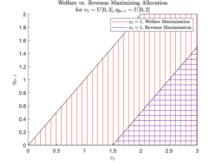
Figure 1: Partition of type space by welfare versus revenue maximizing restricted dependency allocations in Scenario 1, assuming $v_{1}$ and $\eta_{2\leftarrow 1}$ are uniformly distributed on their respective domains $[0,3]$ and $[0,2]$. The shaded regions denote where bidder 1 is allocated the entire dataset ($x_{1}=1$) and the un-shaded regions correspond to the opposite case of $x_{1}=0$.

Impact of Externalities.

To further elucidate the effect of the presence and magnitude of negative externalities on the optimal revenue, we consider the simple setting where each bidder $i\in N$ has value $v_{i}$ distributed uniformly in $[0,\bar{v}_{i}]$, while externality parameters $\eta_{i\leftarrow j}$ are deterministic, for $j\in N\backslash i$. Since the externalities are now common knowledge, Scenario 1 and Scenario 2 are identical. In particular, the optimal mechanism described in Theorem 4.5 and takes a simple form that we now describe.

For uniform type distributions, the virtual valuation functions $\phi_{i}(v_{i})$ are non-decreasing in $v_{i}$. A simple computation shows the expected optimal revenue can thus be expressed as $\sum_{i\in N}R_{i}$, where $R_{i}$ denotes the share of each bidder’s payment induced by the presence of bidder $i$, and is given by

$$R_{i}=\begin{cases}\sum_{j\in N\backslash i}\eta_{j\leftarrow i}&\text{if }\sum_{j\in N\backslash i}\eta_{j\leftarrow i}>\bar{v}_{i},\\[8.0pt] \frac{(\bar{v}_{i}-\sum_{j\in N\backslash i}\eta_{j\leftarrow i})^{2}}{4\bar{v}_{i}}+\sum_{j\in N\backslash i}\eta_{j\leftarrow i}&\text{if }\sum_{j\in N\backslash i}\eta_{j\leftarrow i}\leq\bar{v}_{i}.\end{cases}$$ (13)

Some of comments about this expression are in order:

1. When there are no externalities ($\eta_{j\leftarrow i}=0$ for $j\in N\backslash i$), we recover the revenue of the optimal posted price mechanism $\bar{v}_{i}/4$. Otherwise, we see that $R_{i}$—and thus the overall revenue—is increasing in the externality parameters $\eta_{j\leftarrow i}$ for all $i,j\in N$ with $i\neq j$.

2. Without externalities, the optimal posted price mechanism allocates with probability $1/2$. In contrast, in the presence of externalities, there are two regimes: if $\sum_{j\neq i}\eta_{j\leftarrow i}\leq\bar{v}_{i}$, the optimal mechanism allocates to $i$ with probability $1/2-\sum_{j\neq i}\eta_{j\leftarrow i}/(2\bar{v}_{i})$, otherwise it never allocates.

3. In both regimes—in particular, even when bidder $i$ is not allocated—the optimal mechanism is able to collect at least $\sum_{j\in N\backslash i}\eta_{j\leftarrow i}$, corresponding to the “threat” of allocating to bidder $i$ in the outside option where bidders do not participate.

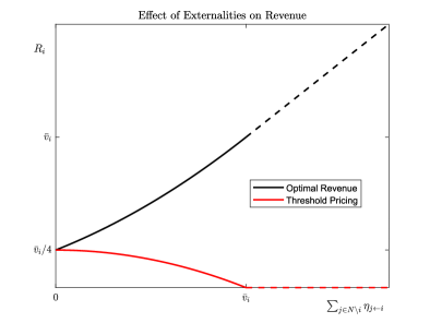
Figure 2: Contribution $R_{i}$ to total revenue due to the presence of bidder $i$ as a function of the externality caused by bidder $i$: $\sum_{j\in N\backslash i}\eta_{j\leftarrow i}$. In black, the value of $R_{i}$ in the optimal mechanism, given by Equation (13). In red, a suboptimal mechanism that only charges the optimal threshold $\tau_{i}$ when allocating to bidder $i$, without extracting additional revenue from bidders $j\neq i$ corresponding to the threat of their outside option.

In summary, the presence of externalities implies that the auctioneer can still extract payments from bidders, even when they do not receive an allocation, while still maintaining IR. It turns out that an auctioneer benefits from greater externalities among bidders: even though increased externalities may lead to fewer allocations and therefore less payments directly driven by these allocations (based on $v_{i}$), the entry fee that the auctioneer charges can make up for and actually exceed this loss in profit. However, if the auctioneer were to only charge the optimal threshold $\tau_{i}=(\bar{v}_{i}+\sum_{j\neq i}\eta_{j\leftarrow i})/2$ upon allocating, without leveraging the outside option, the revenue would in fact be decreasing in the externality parameters. These phenomena are illustrated in Fig. 2.

Acknowledgments

The authors are grateful to Dirk Bergemann, Alessandro Bonatti, Tan Gan, Andreas Haupt, Ali Jadbabaie and Haifeng Xu for fruitful discussions and comments about this work.

Appendix A Prior-independent mechanism

A natural concern with the optimal mechanisms described in Section 4 is that they rely on the knowledge of the type distribution. For example, even in the regular case of Theorem 4.5, the threshold value $\tau_{i}$ of bidder $i$ is described as the zero of the virtual value function which itself depends heavily on the distribution of the type of bidder $i$. In this section, we explore a situation where the type distribution is initially unknown by the mechanism designer and learned over time.

This problem falls within the realm of online stochastic optimization, and more specifically stochastic derivative-free optimization: indeed, the binary decisions of the bidders at each time step let us compute an unbiased estimator of the the expected revenue, which is the only prerequisite of derivative-free optimization procedures. Standard procedures to do so, such as the one described in Flaxman et al. [2005], can then be applied to algorithmically update the thresholds at each time step and provide an upper bound on the rate of convergence to the optimal revenue.

A.1 Problem description

We consider a sequential learning setting in which at each time step, the seller attempts to sell a digital good in an auction with $n$ buyers whose types are drawn from an unknown distribution. The task of the seller is to design an auction mechanism to both satisfy the BNIC and IR constraints at each time step, and also learn the unknown distribution over time and converge to the optimal auction. Specifically, at time step $k\geq 1$:

1. the data seller announces the BNIC and IR mechanism $\mu^{k}=\big{(}\boldsymbol{x}^{k}(\cdot),\boldsymbol{p}^{k}(\cdot))$ which will be used for this time step;

2. a vector of types $\boldsymbol{t}^{k}\in T$ is drawn from the distribution $f$ independently of previous time steps;

3. the good is allocated according to $\boldsymbol{x}(\boldsymbol{t})$ and the seller collects the payments $\boldsymbol{p}(\boldsymbol{t})$.

We emphasize that the underlying distribution $f$ from which the types are drawn is unknown to the seller and so $\mu^{k}$ cannot depend directly on it. However, the seller observes the types reported in previous time steps and can use these observations to inform the design of $\boldsymbol{x}^{k}(\cdot)$ and $\boldsymbol{p}^{k}(\cdot)$. A natural benchmark to evaluate the performance of the chosen sequence of mechanisms is to compare its cumulative revenue to the one which would have been obtained using the optimal auction. Formally, let $\boldsymbol{x}^{\star}(\cdot)$ and $\boldsymbol{p}^{\star}(\cdot)$ denote the revenue-optimal BNIC and IR auction—which depends on the distribution $f$—and define the regret up to time step $K$ by

$$R(K)=\sum_{k=1}^{K}\big{[}\operatorname{\mathrm{Rev}}(\boldsymbol{x}^{\star},\boldsymbol{p}^{\star})-\operatorname{\mathrm{Rev}}(\boldsymbol{x}^{k},\boldsymbol{p}^{k})\big{]}\,,\quad K\geq 1\,.$$

The goal of the data seller is thus to design a sequence of mechanisms which incurs as small a regret as possible.

Remark A.1.

An important assumption in this sequential learning setting is that the buyers’ types are redrawn at each time step from the same distribution and that buyers only strategize within each time step (hence the BNIC and IR constraints) but not across times steps. As such, we ignore intertemporal incentive issues, which could for example lead buyers to misreport their types in order to bias the learning of the distribution that the seller performs over time. We note that an alternative learning model would consider a single-shot auction in which buyers’ types are drawn from identical distributions. In this case, one can still hope to learn the type distribution in a single time step as the number of buyers $n$ goes to infinity. The problem of buyers misreporting their types can be addressed by learning the unknown distribution from a subsample $S\subset N$ of the buyers and then using the learned mechanism only on the remaining $N\backslash S$ buyers. This approach was for example adopted in Goldberg et al. [2006].

A.2 A stochastic optimization solution

We now provide a solution to the sequential learning problem of Section A.1 which leverages the specific structure of the optimal mechanism described in Section 4.2. We will make the following two simplifying assumptions:

• for each buyer $i$, the distribution of her value $v_{i}$ is independent from the distribution of externalities $\boldsymbol{\eta}_{\leftarrow i}$ she causes on others. Furthermore, for all $i$ and $j\in N\backslash i$, the expectation $\operatorname{\mathbb{E}}[\eta_{i\leftarrow j}]$ is known to the seller;

• for each buyer $i$, the function $v_{i}\mapsto v_{i}f_{v_{i}}(v_{i})-(1-F_{v_{i}}(v_{i}))-f_{v_{i}}(v_{i})\sum_{j\in N\backslash i}\operatorname{\mathbb{E}}[\eta_{j\leftarrow i}]$ is non-decreasing.

Under these assumptions, Theorem 4.5 combined with Example 4.6 imply that the revenue-optimal BNIC and IR mechanism is given by

$$x_{i}^{\star}(\boldsymbol{t})=\operatorname{\boldsymbol{1}}\{v_{i}\geq\tau_{i}^{\star}\}\quad\mathrm{and}\quad p_{i}^{\star}(\boldsymbol{t})=\operatorname{\boldsymbol{1}}\{v_{i}\geq\tau_{i}^{\star}\}\cdot\tau_{i}^{\star}+\sum_{j\in N\backslash i}\operatorname{\mathbb{E}}[\eta_{i\leftarrow j}]\cdot F_{v_{j}}(\tau_{j}^{\star})\,,$$

where $\tau_{i}^{\star}\coloneqq\widetilde{\Phi}_{i}^{-1}(0)$ for $\widetilde{\Phi}_{i}$ described in Theorem 4.5. A simple computation further implies that

$$H(\boldsymbol{\tau}^{\star})\coloneqq\operatorname{\mathrm{Rev}}(\boldsymbol{x}^{\star},\boldsymbol{p}^{\star})=\sum_{i\in N}\left[\tau_{i}^{\star}-F_{v_{i}}(\tau_{i}^{\star})\bigg{(}\tau_{i}^{\star}-\sum_{j\in N\backslash i}\operatorname{\mathbb{E}}[\eta_{j\leftarrow i}]\bigg{)}\right]\,.$$ (14)

This formula has a number of important consequences. First, observe that the mechanism obtained by replacing $\boldsymbol{\tau}^{\star}$ by any other vector of thresholds $\boldsymbol{\tau}$ is also BNIC and IR. Since the optimal mechanism is given by the choice of $\boldsymbol{\tau}^{\star}$, optimizing the function $H$ over the choice of $\boldsymbol{\tau}\in\prod_{i\in N}[\text{\@text@baccent{$v$}}_{i},\bar{v}_{i}]$ is sufficient to obtain the optimal mechanism. In other words, the problem of finding the optimal mechanism reduces to the optimization of the function $H$. Furthermore, note that this maximization problem is separable: denoting by $H_{i}$ the summand in (14) we have that $H(\boldsymbol{\tau})=\sum_{i\in N}H_{i}(\tau_{i})$ and hence, the problem reduces to separately maximizing each function $H_{i}$ over the choice of a single-dimension parameter $\tau_{i}$. Finally, observe that the derivative of $H_{i}$ is $h_{i}(\tau_{i})\coloneqq 1-\tau_{i}g_{i}(\tau_{i})-G_{i}(\tau_{i})-g_{i}(\tau_{i})\sum_{j\in N\backslash i}\operatorname{\mathbb{E}}[\eta_{j\leftarrow i}]$ which is non-increasing by assumption. Hence, the function $H_{i}$ is concave.

Learning as stochastic optimization.

The previous observations suggest a natural strategy to learn the optimal auction in the observational model described in Section A.1: using a sequence of posted price mechanisms and iteratively updating the thresholds based on the buyers’ decisions.

Note that when using a posted price mechanism with threshold $\tau_{i}^{k}$ at time step $k$, the only thing we observe from buyer $k$ is her decision to accept or reject the offer, which is the binary random variable $X_{i}^{k}\coloneqq\operatorname{\boldsymbol{1}}\{v_{i}^{k}\geq\tau_{i}^{k}\}$. Hence, the suggested strategy does not even require the buyers to report their entire type but simply relies on the binary observations $(X_{i}^{k})_{i\in N}$ from each time step. From these observations, one can form for each $i\in N$, the quantity

$$H_{i}(\tau_{i}^{k},X_{i}^{k})\coloneqq\tau_{i}^{k}-(1-X_{i}^{k})\bigg{(}\tau_{i}^{k}-\sum_{j\in N\backslash i}\operatorname{\mathbb{E}}[\eta_{j\leftarrow i}]\bigg{)}$$

which is an unbiased estimate of $H_{i}(\tau_{i}^{k})$, that is, $H_{i}(\tau_{i}^{k})=\operatorname{\mathbb{E}}\big{[}H_{i}(\tau_{i}^{k},X_{i}^{k})]$.

This observation conveniently reduces the problem of learning the optimal mechanism to the one of maximizing for each $i\in N$ the concave function $H_{i}(\cdot)$ assuming access to unbiased estimates of $H_{i}(\tau_{i}^{k})$ for a sequence $\tau_{i}^{k}$ of our choice. This problem is exactly what is known in the online learning literature as a stochastic derivative-free optimization problem where the quantity $H_{i}(\tau_{i}^{k},X_{i}^{k})$ plays the role of a zeroth order stochastic oracle. (The stochastic optimization literature distinguishes between first-order stochastic oracles giving unbiased estimates of the gradient of the objective function and zeroth-order oracles given unbiased estimates of the objective function itself.)

Algorithms for stochastic derivative-free optimizations usually take the form of iterative algorithms in which at each time step, the current estimate of the optimal solution is updated based on the previous estimate and the current observation. In our notations, we write:

$$\tau_{i}^{k+1}=\mathrm{Update}(\tau_{i}^{k},X_{i}^{k})$$

where $\mathrm{Update}(\cdot)$ is the update rule given by a stochastic optimization algorithm. We instantiate the stochastic optimization framework in our setting and describe in Algorithm 1 a meta algorithm parametrized by a generic $\mathrm{Update}$ function.

Input: vector of initial thresholds $\boldsymbol{\tau}^{1}$, $\mathrm{Update}$ given a stochastic optimization algorithm

for $k\geq 1$ do

       post vector of thresholds $\boldsymbol{\tau}^{k}$;

       collect buyers’ decisions $X_{i}^{k}=\operatorname{\boldsymbol{1}}\{v_{i}^{k}\geq\tau^{k}_{i}\}$;

       for $i\in N$ do

             if $X_{i}^{k}==1$ then

                   allocate good;

                   collect payment $\tau_{i}^{k}+\sum_{j\in N\backslash i}\operatorname{\mathbb{E}}[\eta_{i\leftarrow j}](1-X_{j}^{k})$;

                  

            else

                   do not allocate good;

                   collect payment $\sum_{j\in N\backslash i}\operatorname{\mathbb{E}}[\eta_{i\leftarrow j}](1-X_{j}^{k})$;

                  

             end if

            $\tau_{i}^{k+1}\leftarrow\mathrm{Update}(\tau_{i}^{k},X_{i}^{k})$;

            

       end for

      

end for

Algorithm 1 A meta online learning algorithm from single-dimensional stochastic optimization

All that remains to do to obtain a concrete bound on the regret of our learning procedure is to choose an $\mathrm{Update}(\cdot)$ function from the stochastic optimization literature. Here, we will not aim for optimal bounds but rather give a simple example of how to instantiate Algorithm 1. A common idea is to estimate the derivative of the objective $H_{i}$ at $\tau_{i}$ by $H_{i}(\tau_{i}+\delta u)u/\delta$ where $u$ is uniformly random over $[-1,1]$. Using this estimate of the derivative in projected gradient-ascent suggests the following simple update rule:

$$\tau_{i}^{k+1}=\tau_{i}^{k}+\gamma\cdot H_{i}(\tau_{i}^{k}+\delta u,X_{i}^{k})u/\delta\,,$$ (15)

where $u$ is uniformly random over $[-1,1]$ and $\gamma$ is the step size parameter. By applying a standard result (see e.g. Flaxman et al. [2005]) we obtain the following proposition.

Proposition A.2.

For any $K\geq 1$, there exists a choice of $\delta$ and $\gamma$ such that using the update rule (15) in Algorithm 1 yields a regret $R(K)=O(K^{3/4})$.

Furthermore, since the revenue is a concave function of the chosen threshold, we recover the standard fact that a bound on the regret implies a bound on the objective function.

Corollary A.3.

Consider the sequence of threshold vectors $(\boldsymbol{\tau}_{k})_{k\geq 1}$ computed by Algorithm 1 with update rule (15) and define $\overline{\boldsymbol{\tau}}_{K}\coloneqq\frac{1}{K}\sum_{k=1}^{K}\boldsymbol{\tau}_{k}$ for $K\geq 1$, and denote by $\operatorname{\mathrm{Rev}}(\overline{\boldsymbol{\tau}}_{K})$ obtained by using the posted price mechanism with thresholds $\overline{\boldsymbol{\tau}}_{K}$. Then for any $K\geq 1$, there exists a choice of $\delta$ and $\gamma$ such that:

$$\operatorname{\mathrm{Rev}}(\boldsymbol{\tau}^{\star})-\operatorname{\mathrm{Rev}}(\overline{\boldsymbol{\tau}}_{K})=O\left(\frac{n}{K^{1/4}}\right)\,.$$

Proof.

. This follows immediately from Proposition A.2 by application of Jensen’s inequality. ∎

Appendix B Linear Externality Models

B.1 Proof of Proposition 2.1

Proof.

By assumption $(p_{1}-p_{2})/(\beta_{1}q_{1}-\beta_{2}q_{2})\geq\text{\@text@baccent{$\alpha$}}>0$, which implies in particular that $p_{1}-p_{2}$ and $\beta_{1}q_{1}-\beta_{2}q_{2}$ have the same sign. Without loss of generality, assume that $p_{1}>p_{2}$ and $\beta_{1}q_{1}>\beta_{2}q_{2}$, otherwise the following proof applies after swapping the role of 1 and 2.

Given the distribution of consumer types,

$$u_{1}(q_{1},q_{2}) =(p_{1}-c_{1})\mathbb{P}\{\alpha:v_{1}(\alpha)>v_{2}(\alpha)\}$$

$$=(p_{1}-c_{1})\text{\@text@baccent{$\alpha$}}(\beta_{1}q_{1}-\beta_{2}q_{2})/(p_{1}-p_{2}).$$

Then taking $\nu_{1}(x_{1},x_{2})=u_{1}(q_{1}+x_{1},q_{2}+x_{2})-u_{1}(q_{1},q_{2})$ and noting the linearity of $u_{1}$ in its arguments, we obtain the result for firm 1. The result for firm 2 follows in a similar manner after observing that $u_{2}(q_{1},q_{2})=(p_{2}-c_{2})(1-\mathbb{P}\{\alpha:v_{1}(\alpha)>v_{2}(\alpha)\})$. ∎

B.2 Proof of Proposition 2.3

Let $\xi=(\alpha_{1},\alpha_{2},c_{1},c_{2},M)$ be the original set of market parameters before data is purchased and production efficiencies are improved, and let $\xi^{\prime}=(\alpha_{1}^{\prime},\alpha_{2}^{\prime},c_{1},c_{2},M)$ be the market parameters after an allocation of data, such that $\alpha_{i}^{\prime}=\alpha_{i}+x_{i}$. For market parameters $\xi$, a standard computation gives the equilibrium production quantity and profits of firm 1:

$$q_{1}^{*}(\xi)=\frac{\alpha_{1}c_{2}-2\alpha_{2}c_{1}+M\alpha_{1}\alpha_{2}}{3{\alpha_{1}}^{2}\alpha_{2}}\quad\text{and}\quad\pi_{1}^{*}(\xi)=(\alpha_{1}q_{1}^{*})^{2}\,,$$

with analogous expressions for those of firm 2 obtained by swapping indices 1 and 2.

We obtain by Taylor expansion the change in equilibrium profits

$$\Delta\pi_{i}(\xi^{\prime},\xi)\coloneqq\pi_{i}^{*}(\xi^{\prime})-\pi_{i}^{*}(\xi)=\sum_{j=1}^{2}\frac{\partial\pi_{i}^{*}}{\partial\alpha_{j}}(\xi)\cdot(\alpha_{j}^{\prime}-\alpha_{j})+O\big{(}\|\xi^{\prime}-\xi\|^{2}\big{)}\,.$$ (16)

Furthermore, a simple computation gives $\frac{\partial\pi_{1}^{*}}{\partial\alpha_{1}}(\xi)=\frac{4c_{1}}{3\alpha_{1}}q_{1}^{*}(\xi)$ and $\frac{\partial\pi_{1}^{*}}{\partial\alpha_{2}}(\xi)=-\frac{2\alpha_{1}c_{2}}{3{\alpha_{2}}^{2}}q_{1}^{*}(\xi)\,.$ Assuming second order terms in (16) are sufficiently small to be ignored, we obtain

$$\Delta\pi_{1}(x_{1},x_{2})=\frac{4c_{1}}{3\alpha_{1}}q_{1}^{*}(\xi)\cdot x_{1}-\frac{2\alpha_{1}c_{2}}{3{\alpha_{2}}^{2}}q_{1}^{*}(\xi)\cdot x_{2}=v_{1}\cdot x_{1}-\eta_{1\leftarrow 2}\cdot x_{2}\,,$$

$$\text{where}\quad v_{1}\coloneqq 4c_{1}q_{1}^{*}(\xi)/(3\alpha_{1})\quad\text{and}\quad\eta_{1\leftarrow 2}\coloneqq 2\alpha_{1}c_{2}q_{1}^{*}(\xi)/(3\alpha_{2}^{2})\,,$$ (17)

and similarly for firm 2. This has the exact same form as (1). In other words, our externality model captures the first order approximation of the change of profit that results from firms acquiring data. This immediately extends to the general case of $n$ firms engaging in Cournot competition.

Appendix C Welfare versus Revenue Maximization in Scenario 1

As stated in Section 4.1, given a distribution function $F_{\eta_{i\leftarrow j}}$ and corresponding density function $f_{\eta_{i\leftarrow j}}$ for the random variable $\eta_{i\leftarrow j}$ supported on $[\text{\@text@baccent{$\eta$}}_{i\leftarrow j},\bar{\eta}_{i\leftarrow j}]$, for $i\neq j\in N$, we define the distribution of $t_{i,j}$ on $[-\bar{\eta}_{i\leftarrow j},-\text{\@text@baccent{$\eta$}}_{i\leftarrow j}]$ by the distribution and density functions

$$F_{i,j}(t_{i,j})=1-F_{\eta_{i\leftarrow j}}(-t_{i,j})=1-F_{\eta_{i\leftarrow j}}(\eta_{i\leftarrow j})$$

$$f_{i,j}(t_{i,j})=f_{\eta_{i\leftarrow j}}(-t_{i,j})=f_{\eta_{i\leftarrow j}}(\eta_{i\leftarrow j}).$$

Further, define for $i,j\in N$ the virtual value function $\Phi_{i,j}(t_{i,j})\coloneqq t_{i,j}-\big{(}1-F_{i,j}(t_{i,j})\big{)}/f_{i,j}(t_{i,j})$. Then for each $i\in N$ and $j\in N\backslash i$, we can express the virtual functions as

$$\Phi_{i,i}(t_{i,i})=v_{i}-\big{(}1-F_{v_{i}}(v_{i})\big{)}/f_{v_{i}}(v_{i})$$

$$\Phi_{i,j}(t_{i,j})=-\eta_{i\leftarrow j}-F_{\eta_{i\leftarrow j}}(\eta_{i\leftarrow j})/f_{\eta_{i\leftarrow j}}(\eta_{i\leftarrow j})$$

Suppose all $v_{i},\eta_{i\leftarrow j}$ for $i\in N,j\in N\backslash i$ are uniformly distributed on their respective domains. The virtual value functions take the forms

$$\Phi_{i,i}(t_{i,i})=2v_{i}-\bar{v_{i}}$$

$$\Phi_{i,j}(t_{i,j})=-2\eta_{i\leftarrow j}+\text{\@text@baccent{$\eta$}}_{i\leftarrow j}$$

The optimal allocation rule (11) then becomes

$$x_{k}(\boldsymbol{t}) =\operatorname{\boldsymbol{1}}\bigg{\{}\sum_{i\in N}\phi_{i,k}(t_{i,k})\geq 0\bigg{\}}$$

$$=\operatorname{\boldsymbol{1}}\bigg{\{}(2v_{k}-\bar{v}_{k})+\sum_{i\in N\backslash k}(-2\eta_{i\leftarrow k}+\text{\@text@baccent{$\eta$}}_{i\leftarrow k})\geq 0\bigg{\}}$$

$$=\operatorname{\boldsymbol{1}}\bigg{\{}v_{k}-\sum_{i\in N\backslash k}\eta_{i\leftarrow k}\geq\frac{\bar{v}_{k}-\sum_{i\in N\backslash k}\text{\@text@baccent{$\eta$}}_{i\leftarrow k}}{2}\bigg{\}}$$

In the case of $n=2$ bidders, bidder $1$’s allocation is

$$x_{1}(\boldsymbol{t})=\operatorname{\boldsymbol{1}}\Big{\{}v_{1}-\eta_{2\leftarrow 1}\geq\frac{\bar{v}_{1}-\text{\@text@baccent{$\eta$}}_{2\leftarrow 1}}{2}\Big{\}}$$

Meanwhile, the welfare-maximizing allocation rule for bidder 1 is

$$x_{1}(\boldsymbol{t})=\operatorname{\boldsymbol{1}}\big{\{}v_{1}-\eta_{2\leftarrow 1}\geq 0\big{\}}.$$

Thus, the revenue-maximizing allocation allocates to bidders less often than does the welfare-maximizing allocation. The optimal mechanism is therefore not efficient in general. This is illustrated in Fig. 1 in Section 5, where the type space for $\boldsymbol{t}$ is partitioned in terms of the welfare-maximizing and revenue-maximizing allocation to bidder 1.

Appendix D Characterizations of IC and IR Mechanisms

An important step towards elucidating the solution structure of the welfare and revenue maximizing mechanisms is to obtain a characterization of the IC and IR constraints. Since our valuation model has the same form as the one in Jehiel et al. [1996, 1999], we rely on the characterizations found in these papers, and state them below for completeness.

D.1 Characterizations in Scenario 1: Incoming Externalities

Recall that each bidder $i$’s type is the vector of the form $t_{i}=v_{i}e_{i}-\sum_{j\in N\backslash i}\eta_{i\leftarrow j}e_{j}\in\mathbb{R}^{n}$ where $e_{k}$ denotes the $k$th vector of the standard basis.

For each bidder $i\in N$, with true type $t_{i}$ and bid $\hat{t}_{i}$, the overall interim expected allocation is defined as $\operatorname{\mathbb{E}}[\boldsymbol{x}(\hat{t}_{i},\boldsymbol{t}_{-i})\nonscript\,|\allowbreak\nonscript\,\mathopen{}t_{i}]=\operatorname{\mathbb{E}}_{\boldsymbol{t}_{-i}}[x(\hat{t}_{i},\boldsymbol{t}_{-i})]$ and the interim expected payment as $\operatorname{\mathbb{E}}[p_{i}(\hat{t}_{i},\boldsymbol{t}_{-i})\nonscript\,|\allowbreak\nonscript\,\mathopen{}t_{i}]=\operatorname{\mathbb{E}}_{\boldsymbol{t}_{-i}}[p_{i}(\hat{t}_{i},\boldsymbol{t}_{-i})]$. Under the given assumption of independent bidder types, the interim expected allocation and payment functions do not depend on bidder $i$’s true type $t_{i}$, so we write $\boldsymbol{y}^{(i)}(\hat{t}_{i})\coloneqq\operatorname{\mathbb{E}}_{\boldsymbol{t}_{-i}}[x(\hat{t}_{i},\boldsymbol{t}_{-i})]$ to indicate the interim expected allocation function and likewise, $q_{i}(\hat{t}_{i})\coloneqq\operatorname{\mathbb{E}}_{\boldsymbol{t}_{-i}}[p_{i}(\hat{t}_{i},\boldsymbol{t}_{-i})]$ for the interim expected payment.

Note that $\boldsymbol{y}^{(i)}$ is a vector field mapping $T_{i}$ to $[0,1]^{n}$. Finally, for every bidder $i\in N$, we define the critical type $\mathring{t}_{i}=\text{\@text@baccent{$v$}}_{i}e_{i}-\sum_{j\in N\backslash i}\text{\@text@baccent{$\eta$}}_{i\leftarrow j}e_{j}$, which will feature in the following IC and IR characterizations. Note $\mathring{t}_{i}$ consists of the type parameter values that are of the smallest magnitude.

Proposition D.1 ([Jehiel et al., 1999, Proposition 1]).

Suppose bidders’ private types are of the form $t_{i}=v_{i}e_{i}-\sum_{j\in N\backslash i}\eta_{i\leftarrow j}e_{j}$ for each bidder $i\in N$. Then the mechanism $(\boldsymbol{x},\boldsymbol{p})$ is BNIC if and only if for each bidder $i\in N$:

1. $\boldsymbol{y}^{(i)}$ is a conservative vector field

2. $\boldsymbol{y}^{(i)}$ is a monotone vector field, that is $\big{\langle}s_{i}-t_{i},\boldsymbol{y}^{(i)}(s_{i})-\boldsymbol{y}^{(i)}(t_{i})\big{\rangle}\geq 0$ for all $s_{i},t_{i}\in T_{i}$.

3. for each type $t_{i}\in T_{i}$, the interim payment is given by

   $$q_{i}(t_{i})=\big{\langle}\boldsymbol{y}^{(i)}(t_{i}),t_{i}\big{\rangle}-\int_{\mathring{t}_{i}}^{t_{i}}\boldsymbol{y}^{(i)}(s_{i})\cdot ds_{i}-C_{i}\,,$$ (18)

   where $C_{i}$ is an arbitrary integration constant whose value sets $V_{i}(\mathring{t}_{i};\mathring{t}_{i})$, the interim utility of bidder $i$ when its type is $\mathring{t}_{i}=\text{\@text@baccent{$v$}}_{i}e_{i}-\sum_{j\in N\backslash i}\text{\@text@baccent{$\eta$}}_{i\leftarrow j}e_{j}$.

We provide the following characterization of interim IR for BNIC mechanisms that maximize revenue.

Proposition D.2.

Suppose private types are of the form $t_{i}=v_{i}e_{i}-\sum_{j\in N\backslash i}\eta_{i\leftarrow j}e_{j}$ for each bidder $i\in N$. Then a revenue-maximizing BNIC mechanism satisfies the interim IR constraint $V_{i}(t_{i};t_{i})\geq V_{i}(\emptyset;t_{i})$ if and only if this condition is satisfied for the critical type $\mathring{t}_{i}=\text{\@text@baccent{$v$}}_{i}e_{i}-\sum_{j\in N\backslash i}\text{\@text@baccent{$\eta$}}_{i\leftarrow j}e_{j}$. Further, the optimal mechanism sets $V_{i}(\mathring{t}_{i};\mathring{t}_{i})=-\sum_{j\in N\backslash i}\text{\@text@baccent{$\eta$}}_{i\leftarrow j}$.

Proof.

We first show that the optimal outside option when bidder $i$ does not participate allocates the digital good to all remaining participants $N\backslash i$. We then show that it suffices to check that interim IR is satisfied for the type $\mathring{t}_{i}$, and finally find the optimal value of the integration constant $V_{i}(\mathring{t}_{i};\mathring{t}_{i})$.

Optimal outside option.

The interim IR constraint is essentially a constraint on the values that the constant $C_{i}=V_{i}(\mathring{t}_{i};\mathring{t}_{i})$ can take. That is, after plugging in the form of the payment rule (18), interim IR can be expressed as:

$$\forall i\in N,\forall t_{i}\in T_{i}\>:\>V_{i}(\mathring{t}_{i};\mathring{t}_{i})+\int_{\mathring{t}_{i}}^{t_{i}}\boldsymbol{y}^{(i)}(s_{i})\cdot ds_{i}\geq V_{i}(\emptyset;t_{i}).$$

Maximizing revenue corresponds to maximizing the expected sum of the interim payments $q_{i}(t_{i})$ and thus of minimizing $V_{i}(\mathring{t}_{i};\mathring{t}_{i})$. Since $\forall t_{i},V_{i}(\emptyset;t_{i})\geq-\sum_{j\in N\backslash i}\eta_{i\leftarrow j}$, we can maximize the feasible region for IR payments by setting $V_{i}(\emptyset;t_{i})=-\sum_{j\in N\backslash i}\eta_{i\leftarrow j}$ with an outside option that allocates to all $j\in N\backslash i$ when $i$ does not participate. That is, we set $x_{j}(\hat{t}_{i}=\emptyset,\hat{\boldsymbol{t}}_{-i})=\operatorname{\boldsymbol{1}}\{i\neq j\}$ for all $i,j\in N$ and $\boldsymbol{t}_{-i}\in T_{-i}$.

Sufficiency of checking interim IR for type $\mathring{t}_{i}$.

If the interim IR constraint holds for all types $t_{i}$, then it clearly holds for the type $\mathring{t}_{i}$. Now suppose that $V_{i}(\mathring{t}_{i};\mathring{t}_{i})\geq V_{i}(\emptyset;\mathring{t}_{i})$. Note that given the optimal outside option of allocating to all remaining bidders, we have that for every $t_{i}\in T_{i}$,

$$V_{i}(\emptyset;t_{i})=-\sum_{j\in N\backslash i}\eta_{i\leftarrow j}.$$ (19)

Then for every $t_{i}\in T_{i}$

$$V_{i}(t_{i};t_{i}) =V_{i}(\mathring{t}_{i};\mathring{t}_{i})+\int_{\mathring{t}_{i}}^{t_{i}}\boldsymbol{y}^{i}(s_{i})\cdot ds_{i}$$

$$\geq V_{i}(\mathring{t}_{i};\mathring{t}_{i})+\sum_{j\in N\backslash i}(-\eta_{i\leftarrow j}-(-\text{\@text@baccent{$\eta$}}_{i\leftarrow j}))$$

$$=V_{i}(\mathring{t}_{i};\mathring{t}_{i})+V_{i}(\emptyset;t_{i})-V_{i}(\emptyset;\mathring{t}_{i})$$

$$\geq V_{i}(\emptyset;t_{i})$$

where the first inequality uses that $t_{i,i}=v_{i}\geq\text{\@text@baccent{$v$}}_{i}$, $t_{i,j}=-\eta_{i\leftarrow j}\leq-\text{\@text@baccent{$\eta$}}_{i\leftarrow j}$ and $\boldsymbol{0}\leq\boldsymbol{y}^{i}\leq 1$ as an allocation vector, the second equality follows from (19), and the last inequality follows from our assumption that $V_{i}(\mathring{t}_{i};\mathring{t}_{i})-V_{i}(\emptyset;\mathring{t}_{i})\geq 0$.

Optimal IR Constant.

Since it suffices to satisfy interim IR for the critical type $\mathring{t}_{i}$, for each $i\in N$, in order to maximize revenue we make the IR constraint bind at $\mathring{t}_{i}$

$$V_{i}(\mathring{t}_{i},\mathring{t}_{i})=V_{i}(\emptyset,\mathring{t}_{i})=-\sum_{j\in N\backslash i}\text{\@text@baccent{$\eta$}}_{i\leftarrow j},$$ (20)

where we plugged in the utility of non-participation of bidder $i$ under the optimal outside option allocation. ∎

D.2 Characterizations in Scenario 2: Outgoing Externalities

Recall that each bidder $i$’s type is the vector of the form $t_{i}=v_{i}e_{i}-\sum_{j\in N\backslash i}\eta_{j\leftarrow i}e_{j}\in\mathbb{R}^{n}$ where $e_{k}$ denotes the $k$th vector of the standard basis. Note that in this scenario, bidder $i$’s expected outside option utility $V_{i}(\emptyset;t_{i})$ does not depend on $t_{i}$.

For each bidder $i\in N$ with true type $t_{i}$ and bid $\hat{t}_{i}$ the interim expected allocation to bidder $i$ is given by $\operatorname{\mathbb{E}}[x_{i}(\hat{t}_{i},\boldsymbol{t}_{-i})\nonscript\,|\allowbreak\nonscript\,\mathopen{}t_{i}]=\operatorname{\mathbb{E}}_{\boldsymbol{t}_{-i}}[x_{i}(\hat{t}_{i},\boldsymbol{t}_{-i})]$ and the interim expected payment for bidder $i$ is $\operatorname{\mathbb{E}}[p_{i}(\hat{t}_{i},\boldsymbol{t}_{-i})\nonscript\,|\allowbreak\nonscript\,\mathopen{}t_{i}]=\operatorname{\mathbb{E}}_{\boldsymbol{t}_{-i}}[p_{i}(\hat{t}_{i},\boldsymbol{t}_{-i})]$. Again, under the given assumption of independent bidder types, the interim functions do not depend on bidder $i$’s true type $t_{i}$, so we define $y_{i}(\hat{t}_{i})\coloneqq\operatorname{\mathbb{E}}[x_{i}(\hat{t}_{i},\boldsymbol{t}_{-i})]$ to be the interim expected allocation function for bidder $i$ and likewise, $q_{i}(\hat{t}_{i})\coloneqq\operatorname{\mathbb{E}}[p_{i}(\hat{t}_{i},\boldsymbol{t}_{-i})]$ to be the interim expected payment function. The following two propositions then characterize BNIC mechanisms, and interim IR for BNIC mechanisms.

Proposition D.3.

Assume that private types are of the form $t_{i}=v_{i}e_{i}-\sum_{j\in N\backslash i}\eta_{j\leftarrow i}e_{j}$ for each bidder $i\in N$. The mechanism $(\boldsymbol{x},\boldsymbol{p})$ is BNIC if and only if for each bidder $i\in N$:

1. there exists a non-decreasing function $\widetilde{y}_{i}:[\text{\@text@baccent{$v$}}_{i},\bar{v}_{i}]\to[0,1]$ such that the interim allocation satisfies $y_{i}(v_{i},\boldsymbol{\eta}_{\leftarrow i})=\widetilde{y}_{i}(v_{i})$ for all but countably many $v_{i}$ and all $\boldsymbol{\eta}_{\leftarrow i}\in\prod_{j\in N\backslash i}[\text{\@text@baccent{$\eta$}}_{j\leftarrow i},\bar{\eta}_{j\leftarrow i}]$.

2. the interim payment function is given by

   $$q_{i}(t_{i})=v_{i}\cdot\widetilde{y}_{i}(v_{i})-\int_{\text{\@text@baccent{$v$}}_{i}}^{v_{i}}\widetilde{y}_{i}(v)dv-\sum_{j\in N\backslash i}\operatorname{\mathbb{E}}\left[\eta_{i\leftarrow j}\cdot x_{j}(t_{i},\boldsymbol{t}_{-i})\nonscript\,\middle|\allowbreak\nonscript\,\mathopen{}t_{i}\right]-C_{i}\,,$$ (21)

   where $C_{i}$ is an arbitrary integration constant.

Furthermore, if these conditions are satisfied, then $V_{i}(t_{i};t_{i})$ is constant with respect to $\boldsymbol{\eta}_{\leftarrow i}$ for almost every $v_{i}\in[\text{\@text@baccent{$v$}}_{i},\bar{v}_{i}]$, and $C_{i}=V_{i}(\text{\@text@baccent{$v$}}_{i}e_{i}-\sum_{j\in N\backslash i}\eta_{j\leftarrow i}e_{j})$ for all $\boldsymbol{\eta}_{\leftarrow i}\in\prod_{j\in N\backslash i}[\text{\@text@baccent{$\eta$}}_{j\leftarrow i},\bar{\eta}_{j\leftarrow i}]$.

Proof.

We first show the necessary implications of IC. Writing Definition 2.8 for $t_{i}=v_{i}e_{i}-\sum_{j\in N\backslash i}\eta_{j\leftarrow i}e_{j}$ as the true type and $\hat{t}_{i}=\hat{v}_{i}e_{i}-\sum_{j\in N\backslash i}\hat{\eta}_{j\leftarrow i}e_{j}$ as the reported type, and then vise versa, i.e.,

$$V_{i}(t_{i};t_{i})\geq V_{i}(\hat{t}_{i};t_{i})$$ (22)

$$V_{i}(\hat{t}_{i};\hat{t}_{i})\geq V_{i}(t_{i};\hat{t}_{i}).$$

Combining the two inequalities yields

$$y_{i}(t_{i})(v_{i}-\hat{v}_{i})\geq y_{i}(\hat{t}_{i})(v_{i}-\hat{v}_{i}).$$

By Lemma D.4 below, this implies condition (i), so we let $\tilde{y}_{i}(v_{i})\coloneqq y_{i}(v_{i}e_{i}-\sum_{j\in N\backslash i}\eta_{j\leftarrow i}e_{j})$ for any $\boldsymbol{\eta}_{\leftarrow i}$.

Note also that the inequality (22), by adding and subtracting the term $\hat{v}_{i}y_{i}(\hat{t}_{i})$ to the right hand side and regrouping terms, can be written equivalently as

$$\forall t_{i},\hat{t}_{i}\in T_{i},$$

$$V_{i}(t_{i};t_{i})\geq V_{i}(\hat{t}_{i};\hat{t}_{i})+(v_{i}-\hat{v}_{i})y_{i}(\hat{t}_{i}).$$ (23)

Then plugging in $t_{i}=v_{i}e_{i}-\sum_{j\in N\backslash i}\eta_{j\leftarrow i}e_{j}$ and $\hat{t}_{i}=v_{i}e_{i}-\sum_{j\in N\backslash i}\hat{\eta}_{j\leftarrow i}e_{j}$ into the preceding inequality yields $V_{i}(t_{i})\geq V_{i}(\hat{t}_{i})$, where we recall that $V_{i}(t_{i})\coloneqq V_{i}(t_{i};t_{i})$. Swapping the roles of $t_{i}$ and $\hat{t}_{i}$ yields the inequality in the opposite direction, and we have that $V_{i}(t_{i})$ is independent of $\boldsymbol{\eta}_{\leftarrow i}$:

$$\forall v_{i},\forall\boldsymbol{\eta}_{\leftarrow i},\forall\hat{\boldsymbol{\eta}}_{\leftarrow i},\ V_{i}\left(v_{i}e_{i}-\sum_{j\in N\backslash i}\eta_{j\leftarrow i}e_{j}\right)=V_{i}\left(v_{i}e_{i}-\sum_{j\in N\backslash i}\hat{\eta}_{j\leftarrow i}e_{j}\right).$$

We henceforth define $\tilde{V}_{i}(v_{i})\coloneqq V_{i}(v_{i}e_{i}-\sum_{j\in N\backslash i}\eta_{j\leftarrow i}e_{j})$ for any $\boldsymbol{\eta}_{\leftarrow i}$.

To prove (ii), we first note that $V_{i}(t_{i})$ is convex in $v_{i}$. (22) implies that

$$V_{i}(t_{i},t_{i})=\max_{\hat{t}_{i}\in T_{i}}y_{i}(\hat{t}_{i})v_{i}-\sum_{j\in N\backslash i}\operatorname{\mathbb{E}}\left[\eta_{i\leftarrow j}\cdot x_{j}(\hat{t}_{i},\boldsymbol{t}_{-i})\nonscript\,\middle|\allowbreak\nonscript\,\mathopen{}t_{i}\right]-q_{i}(\hat{t}_{i}).$$

Thus, $V_{i}(t_{i})$ is the maximum of a family of linear functions of $v_{i}$ and is thus convex in $v_{i}$. (D.2) implies that $y_{i}(t_{i})=\tilde{y}_{i}(v_{i})$ is a subderivative of $V_{i}(t_{i})=\tilde{V}_{i}(v_{i})$. In fact, since $\tilde{V}_{i}$ is convex in $v_{i}$, it is differentiable almost everywhere and

$$y_{i}(t_{i})=\tilde{y}_{i}(v_{i})=\frac{\partial\tilde{V}_{i}(v_{i})}{\partial v_{i}}\text{a.e.}$$

Further, this implies that

$$\tilde{V}_{i}(v_{i})=\int_{\text{\@text@baccent{$v$}}_{i}}^{v_{i}}\tilde{y}_{i}(v)dv+\tilde{V}_{i}(\text{\@text@baccent{$v$}}_{i})$$ (24)

Now plugging in the following expression for $V_{i}$,

$$V_{i}(t_{i})=v_{i}\cdot y_{i}(t_{i})-\sum_{j\in N\backslash i}\operatorname{\mathbb{E}}\left[\eta_{i\leftarrow j}\cdot x_{j}(t_{i},\boldsymbol{t}_{-i})\nonscript\,\middle|\allowbreak\nonscript\,\mathopen{}t_{i}\right]-q_{i}(\hat{t}_{i})\,.$$

and solving for $q_{i}(t_{i})$, we get

$$q_{i}(t_{i})=v_{i}\tilde{y}_{i}(v_{i})-\int_{\text{\@text@baccent{$v$}}_{i}}^{v_{i}}\tilde{y}_{i}(v)dv-\sum_{j\in N\backslash i}\operatorname{\mathbb{E}}\left[\eta_{i\leftarrow j}\cdot x_{j}(t_{i},\boldsymbol{t}_{-i})\nonscript\,\middle|\allowbreak\nonscript\,\mathopen{}t_{i}\right]-\tilde{V}_{i}(\text{\@text@baccent{$v$}}_{i}).$$ (25)

We next show the sufficiency of the conditions for IC, by proving the equivalent condition for IC, (D.2). We have that $\forall i\in N,\forall t_{i}=v_{i}e_{i}-\sum_{j\in N\backslash i}\eta_{j\leftarrow i}e_{j},\forall\hat{t}_{i}=\hat{v}_{i}e_{i}-\sum_{j\in N\backslash i}\hat{\eta}_{j\leftarrow i}e_{j},$

$$V_{i}(t_{i})-V_{i}(\hat{t}_{i}) =\int_{\hat{v}_{i}}^{v_{i}}\tilde{y}_{i}(v)dv$$

$$\geq\tilde{y}_{i}(\hat{v}_{i})(v_{i}-\hat{v}_{i})$$

where the first equality follows from (24) and the inequality follows from condition (i) that $\tilde{y}_{i}(v_{i})$ is increasing in $v_{i}$.

Lemma D.4.

For $d\geq 1$, let $f:\mathbb{R}\times\mathbb{R}^{d}\rightarrow\mathbb{R}$ be a bounded function such that

$$f(x_{2},y_{2})(x_{2}-x_{1})\geq f(x_{1},y_{1})(x_{2}-x_{1}),\quad(x_{1},y_{1}),(x_{2},y_{2})\in\mathbb{R}\times\mathbb{R}^{d}\,.$$

Then, there exists a non-decreasing function $\tilde{f}:\mathbb{R}\to\mathbb{R}$ such that $f(x,y)=\tilde{f}(x)$ for all $y\in\mathbb{R}^{d}$ and for all but at most countably many values of $x\in\mathbb{R}$.

By a rescaling and shifting of $f$ we assume without loss of generality that the range of $f$ is contained in $[0,1]$. Let us now define $S\coloneqq\{x\in\mathbb{R}:\exists y_{1},y_{2}\in\mathbb{R}^{d}\text{ s.t. }f(x,y_{2})\neq f(x,y_{1})\}$ and for $n\geq 1$, $S_{n}\coloneqq\{x\in\mathbb{R}:\exists y_{1},y_{2}\in\mathbb{R}^{d}\text{ s.t. }f(x,y_{2})-f(x,y_{1})\geq 1/n\}$ and observe that $S=\cup_{n\geq 1}S_{n}$.

We now prove that $|S_{n}|\leq n$. Indeed, consider $x_{1}<\dots<x_{m}$, $m$ distinct points in $S_{n}$, and for each $k\in[m]$, $y_{k}^{1},y_{k}^{2}$ such that $f(x_{k},y_{k}^{2})-f(x_{k},y_{k}^{1})\geq 1/n$. Then

$$\frac{m}{n} \leq\sum_{k=1}^{m}\big{[}f(x_{k},y_{k}^{2})-f(x_{k},y_{k}^{1})\big{]}$$

$$=f(x_{m},y_{m}^{2})-\sum_{k=2}^{m}[f(x_{k},y_{k}^{1})-f(x_{k-1},y_{k-1}^{2})]-f(x_{1},y_{1}^{1})$$

$$\leq f(x_{m},y_{m}^{2})-f(x_{1},y_{1}^{1})\leq 1\,,$$

where the first inequality uses the definition of $S_{n}$, the equality is summation by parts, the second inequality uses our assumption on $f$ and the last inequality uses that the range of $f$ is contained in $[0,1]$. It then follows that $m\leq n$, i.e. that $|S_{n}|\leq n$, which in turn implies that $S$ is countable.

Define $\tilde{f}$ by $\tilde{f}(x)=f(x,y)$ for $x\notin S$ (this definition does not depend on the choice of $y$ by definition of $S$). Then our assumption on $f$ immediately implies that $\tilde{f}$ is non-decreasing on $\mathbb{R}\backslash S$. We can thus extend $\tilde{f}$ to a non-decreasing function defined over all of $\mathbb{R}$ (for example by right continuity). The resulting $\tilde{f}$ satisfies the stated requirements. ∎

Proposition D.5.

Suppose private types are of the form $t_{i}=v_{i}e_{i}-\sum_{j\in N\backslash i}\eta_{j\leftarrow i}e_{j}\in T_{i}$ for each bidder $i\in N$. Then a BNIC mechanism satisfies the interim IR constraint $V_{i}(t_{i};t_{i})\geq V_{i}(\emptyset;t_{i})$ for all $t_{i}\in T_{i}$, if and only if this condition is satisfied for some type of the form $\text{\@text@baccent{$v$}}_{i}e_{i}-\sum_{j\in N\backslash i}\eta_{j\leftarrow i}e_{j}$, where $\eta_{j\leftarrow i}\in[\text{\@text@baccent{$\eta$}}_{j\leftarrow i},\bar{\eta}_{j\leftarrow i}]$ for $j\in N\backslash i$.

Proof.

Note that BNIC implies (24), and since $\tilde{y}_{i}\geq 0$, we have that $V_{i}(t_{i};t_{i})\geq\tilde{V}_{i}(\text{\@text@baccent{$v$}}_{i})$ for all $t_{i}\in T_{i}$. Since $V_{i}(\emptyset;t_{i})$ is independent with respect to $t_{i}$, it is both necessary and sufficient for IR to hold that the IR condition holds for some type of the form $\text{\@text@baccent{$v$}}_{i}e_{i}-\sum_{j\in N\backslash i}\eta_{j\leftarrow i}e_{j}$, for each bidder $i\in N$. ∎

Appendix E Welfare Maximization

E.1 Proof of Theorem 3.1

We show that the specified VCG mechanism (1) satisfies DSIC, (2) ex-post IR, and (3) uses nonnegative payments. Recall that in this setting, private types are of the form $t_{i}=v_{i}e_{i}-\sum_{j\in N\backslash i}\eta_{i\leftarrow j}$, for $i\in N$.

1. For all $i\in N$ and all $t_{i},\hat{t}_{i}\in\Theta_{i},\boldsymbol{t}_{-i},\hat{\boldsymbol{t}}_{-i}\in\Theta_{-i}$, let us temporarily define the following quantities for ease of notation. Note the only quantity varying in the following terms is bidder $i$’s bid, while all other parameters are fixed.

   $$x_{i}\coloneqq x_{i}(t_{i},\hat{\boldsymbol{t}}_{-i}),\hat{x}_{i}\coloneqq x_{i}(\hat{t}_{i},\hat{\boldsymbol{t}}_{-i})$$

   $$x_{j}\coloneqq x_{j}(t_{i},\hat{\boldsymbol{t}}_{-i}),\hat{x}_{j}\coloneqq x_{j}(\hat{t}_{i},\hat{\boldsymbol{t}}_{-i}),x_{j}^{i}\coloneqq x_{j}(t_{i}=\emptyset,\boldsymbol{t}_{-i}),\,\text{ for }j\in N\backslash i$$

   $$p_{i}\coloneqq p_{i}(t_{i},\hat{\boldsymbol{t}}_{-i}),\hat{p}_{i}\coloneqq p_{i}(\hat{t}_{i},\hat{\boldsymbol{t}}_{-i})$$

   $$W_{i}\coloneqq v_{i}-\sum_{j\in N\backslash i}\eta_{j\leftarrow i},\hat{W}_{i}\coloneqq\hat{v}_{i}-\sum_{j\in N\backslash i}\eta_{j\leftarrow i}$$

   $$W_{j}=v_{j}-\sum_{k\in N\backslash j}\eta_{k\leftarrow j},\hat{W}_{j}\coloneqq v_{j}-\sum_{k\in N\backslash\{j,i\}}\eta_{k\leftarrow j}-\hat{\eta}_{i\leftarrow j}\text{, for }j\in N\backslash i$$

   We show that the following expression is nonnegative, which is precisely the statement of DSIC:

   $$u_{i}\big{(}\boldsymbol{x}(t_{i},\hat{\boldsymbol{t}}_{-i}),p_{i}(t_{i},\hat{\boldsymbol{t}}_{-i});\boldsymbol{t}\big{)}-u_{i}\big{(}\boldsymbol{x}(\hat{\boldsymbol{t}}),p_{i}(\hat{\boldsymbol{t}});\boldsymbol{t}\big{)}$$

   $$=(x_{i}-\hat{x}_{i})v_{i}-\sum_{j\in N\backslash i}\eta_{i\leftarrow j}(x_{j}-\hat{x}_{j})$$

   $$\quad\quad\quad\quad\quad\quad+\sum_{j\in N\backslash i}(-W_{j}^{i}(x_{j}^{i}-x_{j})-\eta_{j\leftarrow i}x_{i}+W_{j}^{i}(x_{j}^{i}-\hat{x}_{j})-\eta_{j\leftarrow i}\hat{x}_{i})$$

   $$=(x_{i}-\hat{x}_{i})(v_{i}-\sum_{j\in N\backslash i}\eta_{j\leftarrow i})+\sum_{j\in N\backslash i}(W_{j}^{i}-\eta_{i\leftarrow j})(x_{j}-\hat{x}_{j})$$

   $$=(\operatorname{\boldsymbol{1}}\{W_{i}\geq 0\}-\operatorname{\boldsymbol{1}}\{\hat{W}_{i}\geq 0\})W_{i}+\sum_{j\in N\backslash i}W_{j}(\operatorname{\boldsymbol{1}}\{W_{j}\geq 0\}-\operatorname{\boldsymbol{1}}\{\hat{W}_{j}\geq 0\})$$

   $$\geq 0.$$

   For the first equality we used the second expression of the payment rule in (5), we regrouped terms and used the definitions of $W_{i},W_{j}$ for the second and third equalities. The final inequality holds because

   $$\operatorname{\boldsymbol{1}}\{W_{i}\geq 0\}-\operatorname{\boldsymbol{1}}\{\hat{W}_{i}\geq 0\}=\begin{cases}1&\text{if $W_{i}\geq 0$ and $\hat{W}_{i}<0$}\\ -1&\text{if $W_{i}<0$ and $\hat{W}_{i}\geq 0$}\\ 0&\text{otherwise,}\end{cases}$$

   and likewise for $\operatorname{\boldsymbol{1}}\{W_{j}\geq 0\}-\operatorname{\boldsymbol{1}}\{\hat{W}_{j}\geq 0\}$, implying that each term in the summation is nonnegative.

2. Let $\boldsymbol{t}$ be an arbitrary type realization. Showing ex-post IR is equivalent to showing

   $$v_{i}x_{i}-\sum_{j\in N\backslash i}\eta_{i\leftarrow j}x_{j}-p_{i}\geq u_{i}(\boldsymbol{x}(\emptyset,\boldsymbol{t}_{-i}),p_{i}(\emptyset,\boldsymbol{t}_{-i});\boldsymbol{t})=-\sum_{j\in N\backslash i}\eta_{i\leftarrow j}x_{j}^{i}.$$

   Plugging in the payment rule, we get the equivalent inequality

   $$v_{i}x_{i}-\sum_{j\in N\backslash i}\left(W_{j}^{i}(x_{j}^{i}-x_{j})+\eta_{j\leftarrow i}x_{i}\right)\geq-\sum_{j\in N\backslash i}\eta_{i\leftarrow j}(x_{j}^{i}-x_{j})$$

   Rearranging and regrouping terms, we get that this is equivalent to

   $$W_{i}x_{i}-\sum_{j\in N\backslash i}W_{j}(x_{j}^{i}-x_{j})\geq 0$$

   Since $x_{i}=\operatorname{\boldsymbol{1}}\{W_{i}\geq 0\}$, the first term is always nonnegative. The terms in the summation are likewise nonnegative since

   $$x_{j}^{i}-x_{j}=\begin{cases}+1&\text{if $W_{j}\geq 0$ and $W_{j}^{i}<0$}\\ -1&\text{if $W_{j}<0$ and $W_{j}^{i}\geq 0$}\\ 0&\text{otherwise}.\end{cases}$$

   Thus, the IR constraint is satisfied for all types $\boldsymbol{t}$.

3. Let $\boldsymbol{t}$ be an arbitrary type realization. Note that since $\eta_{j\leftarrow i}\geq 0$, we can lower bound the payments in (5) by

   $$p_{i}\geq\sum_{j\in N\backslash i}W_{j}^{i}\big{(}\operatorname{\boldsymbol{1}}\{W_{j}^{i}\geq 0\}-\operatorname{\boldsymbol{1}}\{W_{j}\geq 0\}\big{)}.$$

   We have that

   $$\operatorname{\boldsymbol{1}}\{W_{j}^{i}\geq 0\}-\operatorname{\boldsymbol{1}}\{W_{j}\geq 0\}=\begin{cases}+1&\text{if $W_{j}^{i}\geq 0$ and $W_{j}<0$}\\ -1&\text{if $W_{j}^{i}<0$ and $W_{j}\geq 0$}\\ 0&\text{otherwise.}\end{cases}$$

   Matching up the cases, we get that $p_{i}\geq 0$, so payments are nonnegative.

E.2 Proof of Proposition 3.2

Consider a uniform type distribution $F$ over two points: $\boldsymbol{t}^{a}=(\hat{v}_{1},\boldsymbol{\eta}_{1\to}^{a},\hat{\boldsymbol{t}}_{-1})$ and $\boldsymbol{t}^{b}=(\hat{v}_{1},\boldsymbol{\eta}_{1\to}^{b},\hat{\boldsymbol{t}}_{-1})$, where $\hat{v}_{1}\in\mathbb{R}_{\geq 0}$ and $\hat{\boldsymbol{t}}_{-1}=(t_{j})_{j\neq 1}$ are arbitrary, fixed values. We choose $\boldsymbol{\eta}_{1\to}^{a}=(\eta_{j\leftarrow 1})_{j\neq 1}$ and $\boldsymbol{\eta}_{1\to}^{a}=(\eta_{j\leftarrow 1})_{j\neq 1}$ satisfying

$$\sum_{j\in N\backslash 1}\eta_{j\leftarrow 1}^{a}<\hat{v}_{1}<\sum_{j\in N\backslash 1}\eta_{j\leftarrow 1}^{b}.$$ (26)

For instance, we can take $\boldsymbol{\eta}_{1\to}^{a}=\boldsymbol{0}$ and $\boldsymbol{\eta}_{1\to}^{b}=2\hat{v}_{1}\boldsymbol{1}$.

Let us consider an allocation $\boldsymbol{x}(\cdot)\in\mathcal{X}_{BNIC}(F)$. By Proposition D.3 there exists a non-decreasing function $\tilde{y}$ such that $\forall\boldsymbol{t}\in T$, $x_{1}(\boldsymbol{t})=\operatorname{\mathbb{E}}[x_{1}(\boldsymbol{t})|t_{1}]=\tilde{y}(v_{1})$. However, under the distribution $F$, $v_{i}$ only takes the single value $\hat{v}_{i}$, so the function $x_{1}(\boldsymbol{t})$ must be constant-valued. We now consider two cases depending on the sign of this constant value.

If $x_{1}(\boldsymbol{t})>0$ for all $\boldsymbol{t}\in T$, then define $\boldsymbol{y}(\cdot)$ by $y_{1}(\boldsymbol{t})=0$ and $y_{j}(\boldsymbol{t})=x_{j}(\boldsymbol{t})$ for all $j\neq 1$. We have that

$$SW(x;\boldsymbol{t}^{b})-SW(y;\boldsymbol{t}^{b})=\Big{(}\hat{v}_{1}-\sum_{j\in N\backslash i}\eta_{j\leftarrow 1}^{b}\Big{)}\big{(}(x_{1}(\boldsymbol{t}^{b})-y_{1}(\boldsymbol{t}^{b})\big{)}<0$$

where the strict inequality follows from (26) and that $\forall\boldsymbol{t},x_{1}(\boldsymbol{t})>0=y_{1}(\boldsymbol{t})$.

Likewise, if $x_{1}(\boldsymbol{t})\leq 0$ for all $\boldsymbol{t}\in T$, define $\boldsymbol{y}(\cdot)$ by $y_{1}(\boldsymbol{t})=1$ and $y_{j}(\boldsymbol{t})=x_{j}(\boldsymbol{t})$ for all $j\neq 1$. Then

$$SW(x;\boldsymbol{t}^{a})-SW(y;\boldsymbol{t}^{a})=\Big{(}\hat{v}_{1}-\sum_{j\in N\backslash 1}\eta_{j\leftarrow 1}^{a}\Big{)}\big{(}x_{1}(\boldsymbol{t}^{a})-y_{1}(\boldsymbol{t}^{a})\big{)}<0$$

where the strict inequality follows from (26) and that $\forall\boldsymbol{t},x_{1}(\boldsymbol{t})\leq 0<1=y_{1}(\boldsymbol{t})$.

Thus, we have shown that for any BNIC allocation, there exists some type realization for which a different BNIC allocation rule yields strictly greater social welfare. This is precisely the statement in (6).

E.3 Proof of Theorem 3.3

Allocations.

To solve for the form of the expected welfare maximizing allocation function satisfying the IC constraints, we first express the objective in terms of the interim allocations $y_{i}(t_{i})$. Defining $W_{i}(t_{i})\coloneqq v_{i}-\sum_{j\in N\backslash i}\eta_{j\leftarrow i}$ as in Section 3.1, we have

$$\operatorname{\mathbb{E}}\big{[}\operatorname{\mathrm{SW}}(\boldsymbol{x};\boldsymbol{t})\big{]}=\sum_{i\in N}\operatorname{\mathbb{E}}[W_{i}(t_{i})x_{i}(\boldsymbol{t})]=\sum_{i\in N}\operatorname{\mathbb{E}}\big{[}\operatorname{\mathbb{E}}[W_{i}(t_{i})x_{i}(t_{i},\boldsymbol{t}_{-i})\nonscript\,|\allowbreak\nonscript\,\mathopen{}t_{i}]\big{]}=\sum_{i\in N}\operatorname{\mathbb{E}}[W_{i}(t_{i})y_{i}(t_{i})]\,.$$

Now, the BNIC characterization from Proposition D.3 implies that there must exist functions $\widetilde{y}_{i}:[\text{\@text@baccent{$v$}}_{i},\bar{v}_{i}]\to[0,1]$ such that $y_{i}(t_{i})=\widetilde{y}_{i}(v_{i})$ for almost all $t_{i}\in T_{i}$. Plugging in this representation above, we get

$$\operatorname{\mathbb{E}}[\operatorname{\mathrm{SW}}(\boldsymbol{x};\boldsymbol{t})]=\sum_{i\in N}\operatorname{\mathbb{E}}[W_{i}(t_{i})\widetilde{y}_{i}(v_{i})]=\sum_{i\in N}\operatorname{\mathbb{E}}\big{[}\widetilde{y}_{i}(v_{i})\operatorname{\mathbb{E}}[W_{i}(t_{i})\nonscript\,|\allowbreak\nonscript\,\mathopen{}v_{i}]\big{]}\,.$$

Noting the linearity of the objective in $\widetilde{y}_{i}$, we find that the optimal allocation rule is

$$\widetilde{y}_{i}(v_{i})=\operatorname{\boldsymbol{1}}\big{\{}\operatorname{\mathbb{E}}[W_{i}(t_{i})\nonscript\,|\allowbreak\nonscript\,\mathopen{}v_{i}]\geq 0\big{\}}=\operatorname{\boldsymbol{1}}\bigg{\{}v_{i}-\sum_{j\in N\backslash i}\operatorname{\mathbb{E}}[\eta_{j\leftarrow i}\nonscript\,|\allowbreak\nonscript\,\mathopen{}v_{i}]\geq 0\bigg{\}}\,.$$

Under the given assumptions, $\widetilde{y}_{i}(v_{i})$ is non-decreasing in $v_{i}$, so BNIC is satisfied. Finally, note that since we can express the objective function and constraints only in terms of the interim allocations $y_{i}$ for $i\in N$, we can without loss of generality for all $i\in N$, set the allocation rule $x_{i}(\boldsymbol{t})=y_{i}(t_{i})=\widetilde{y}_{i}(v_{i})$.

Payments.

The induced interim payment rule $q_{i}(t_{i})=\operatorname{\mathbb{E}}[p_{i}(\boldsymbol{t})\nonscript\,|\allowbreak\nonscript\,\mathopen{}t_{i}]$ associated with $y_{i}$ as derived in Proposition D.3, condition (ii) is

$$q_{i}(t_{i}) =v_{i}\cdot y_{i}(t_{i})-\int_{\text{\@text@baccent{$v$}}_{i}}^{v_{i}}\widetilde{y}_{i}(v)dv-\sum_{j\in N\backslash i}\operatorname{\mathbb{E}}\big{[}\eta_{i\leftarrow j}x_{j}(t_{i},t_{-i})\nonscript\,\big{|}\allowbreak\nonscript\,\mathopen{}t_{i}\big{]}-C_{i}\,.$$ (27)

Recall that the constant term $C_{i}$ is set such that the payment function satisfies IR. By Proposition D.5, it suffices to check IR for any type of the form $t_{i}=(\text{\@text@baccent{$v$}}_{i},\boldsymbol{\eta}_{\leftarrow i})$, for each $i\in N$. Here, bidder $i$’s expected utility $V_{i}(\emptyset;t_{i})$ if she doesn’t participate is the sum of the externalities effects from the allocations $x_{j}(t_{i}=\emptyset,\boldsymbol{t}_{-i})$ in the welfare-maximizing auction run with the remaining set $N\backslash i$ of bidders, and given the assumption of $v_{j}\mapsto v_{j}-\sum_{k\in N\backslash\{j,i\}}\operatorname{\mathbb{E}}[\eta_{k\leftarrow j}|v_{j}]$ non-decreasing, we have

$$V_{i}(\emptyset;t_{i}) =\sum_{j\in N\backslash i}\operatorname{\mathbb{E}}\left[\eta_{i\leftarrow j}x_{j}(t_{i}=\emptyset,\boldsymbol{t}_{-i})(\boldsymbol{t}_{-i})\right]$$

$$=\quad\sum_{j\in N\backslash i}\operatorname{\mathbb{E}}\Bigg{[}\eta_{i\leftarrow j}\operatorname{\boldsymbol{1}}\bigg{\{}v_{j}\geq\sum_{\mathclap{k\in N\backslash\{{j,i}\}}}\operatorname{\mathbb{E}}[\eta_{k\leftarrow j}|v_{j}]\bigg{\}}\Bigg{]}$$ (28)

Then any payment rule of the form (27) with the constant $C_{i}$ set greater than or equal to $V_{i}(\emptyset;t_{i})$ in (E.3) will give us an IR mechanism.

Finally, since the objective function and constraints can be expressed solely in terms of the interim payments $q_{i}$, we can set $p_{i}(\boldsymbol{t})\coloneqq q_{i}(t_{i})$. Under the given assumption that $v_{i}\mapsto v_{i}-\sum_{j\in N\backslash i}\operatorname{\mathbb{E}}[\eta_{j\leftarrow i}|v_{i}]$ is non-decreasing, we can re-express the allocation rule as

$$x_{i}(\boldsymbol{t})=y_{i}(t_{i})=\operatorname{\boldsymbol{1}}\bigg{\{}v_{i}\geq\sum_{\mathclap{j\in N\backslash i}}\operatorname{\mathbb{E}}[\eta_{j\leftarrow i}\nonscript\,|\allowbreak\nonscript\,\mathopen{}v_{i}]\bigg{\}}=\operatorname{\boldsymbol{1}}\{v_{i}\geq\tau_{i}\}$$ (29)

The integral term in (27) then becomes

$$\int_{\text{\@text@baccent{$v$}}_{i}}^{v_{i}}\operatorname{\boldsymbol{1}}\{v\geq\tau_{i}\}dv =(v_{i}-\tau_{i})\cdot\operatorname{\boldsymbol{1}}\{v_{i}\geq\tau_{i}\}=(v_{i}-\tau_{i})\cdot y_{i}(t_{i})$$

Plugging in the above expression, along with the form of the allocation (29), into (27) completes the proof.

Appendix F Revenue Maximization

F.1 Proof of Proposition 4.1

An instance of the $n$-item auction is a distribution $F$ over $n$-tuples of item valuations. We make the standard assumption that item valuations are non-negative (i.e. the marginals of $F$ are supported on $\mathbb{R}_{\geq 0}$), and denote by $\mathcal{V}$ the support of $F$. Let $s:\mathbb{R}^{n}\to\mathbb{R}^{n}$ be the involution that flips the signs of all but the first of its input’s coordinates: $s(v)=(v_{1},-v_{2},\dots,-v_{n})$. We define the distribution $\widetilde{F}=s_{*}(F)\otimes\delta_{0}\otimes\cdots\otimes\delta_{0}$ over type profiles in the digital good auction, where $s_{*}(F)$ is the pushforward of $F$ through $s$ and $\delta_{0}$ denotes the Dirac measure at $0\in\mathbb{R}^{n}$. In other words, the support of $\widetilde{F}$ is $T=s(\mathcal{V})\times\{0\}\times\cdots\times\{0\}$, and $\boldsymbol{t}$ is distributed according to $\widetilde{F}$ iff $s^{-1}(t_{1})=s(t_{1})$ is distributed according to $F$ and $t_{2},\dots,t_{n}$ are constant equal to $0\in\mathbb{R}^{n}$.

Let $(x,p)$ be a mechanism for the $n$-item auction, with $x:\mathcal{V}\to[0,1]^{n}$ describing the allocation probabilities of each of the $n$ items, and $p:\mathcal{V}\to\mathbb{R}_{\geq 0}$ being the corresponding payment function. For each $(x,p)$, we define a corresponding mechanism $(\tilde{x},\tilde{p})$ for the $n$-player digital good auction as follows: for each $t\in T$,

$$\begin{cases}\tilde{x}_{1}(t)=x_{1}\big{(}s(t_{1})\big{)}\\ \tilde{p}_{1}(t)=p\big{(}s(t_{1})\big{)}\end{cases}\text{and for $2\leq i\leq n$,}\quad\begin{cases}\tilde{x}_{i}(t)=1-x_{i}\big{(}s(t_{1})\big{)}\\ \tilde{p}_{i}(t)=0\end{cases}.$$ (30)

Then,

$$\begin{split}&\forall(v,v^{\prime})\in\mathcal{V}^{2},\;\left\langle v,x(v)\right\rangle-p(v)\geq\left\langle v,x(v^{\prime})\right\rangle-p(v^{\prime})\\ \iff&\forall(t_{1},t_{1}^{\prime})\in T_{1}^{2},\;\left\langle s(t_{1}),x\big{(}s(t_{1})\big{)}\right\rangle-p\big{(}s(t_{1})\big{)}\geq\left\langle s(t_{1}),x\big{(}s(t_{1}^{\prime})\big{)}\right\rangle-p\big{(}s(t_{1}^{\prime})\big{)}\\ \iff&\forall(t_{1},t_{1}^{\prime})\in T_{1}^{2},\;\begin{aligned} &\,t_{11}\tilde{x}_{1}(t_{1},0)-\sum_{i=2}^{n}t_{1i}\big{(}1-\tilde{x}_{i}(t_{1},0)\big{)}-\tilde{p}_{1}(t_{1},0)\\ \geq&\,t_{11}\tilde{x}_{1}(t_{1}^{\prime},0)-\sum_{i=2}^{n}t_{1i}\big{(}1-\tilde{x}_{i}(t_{1}^{\prime},0)\big{)}-\tilde{p}_{1}(t_{1}^{\prime},0)\end{aligned}\\ \iff&\forall(t_{1},t_{1}^{\prime})\in T_{1}^{2},\;\left\langle t_{1},\tilde{x}(t_{1},0)\right\rangle-\tilde{p}_{1}(t_{1},0)\geq\left\langle t_{1},\tilde{x}(t_{1}^{\prime},0)\right\rangle-\tilde{p}_{1}(t_{1}^{\prime},0).\end{split}$$ (31)

We used that $s$ induces a bijection from $T_{1}\coloneqq s(\mathcal{V})$ to $\mathcal{V}$ in the first equivalence, and the definitions of $s$, $\tilde{x}$ and $\tilde{p}$ in the second. Adding $\sum_{i=2}^{n}t_{1i}$ to both sides of the inequality yields the third equivalence. Recall that under $\widetilde{F}$, each of the type vectors $t_{2},\dots,t_{n}$ is supported on $0\in\mathbb{R}^{n}$ a.s., hence truthful reporting of players $2$ to $n$ is trivially guaranteed. Finally, (31) shows that $(x,p)$ is IC iff $(\tilde{x},\tilde{p})$ satisfies the IC constraint of player $1$.

We now look at the participation constraints. In the $n$-item auction, non-participation implies that the buyer is allocated no item (and no payment is collected), resulting in a vanishing reservation utility. In the $n$-player digital good auction, we set the allocation of player $1$ in case of non-participation to be $\tilde{x}_{i}(\emptyset,0)=\operatorname{\boldsymbol{1}}\{i\neq 1\}$, which results in the worst possible reservation utility $\sum_{i=2}^{n}t_{1i}$ for type $t_{1}$. Then, following the same steps as in (31):

$$\forall v\in\mathcal{V},\;\left\langle v,x(v)\right\rangle-p(v)\geq 0$$

$$\iff \forall t_{1}\in T_{1},\;\left\langle s(t_{1}),x\big{(}s(t_{1})\big{)}\right\rangle-p\big{(}s(t_{1})\big{)}\geq 0$$

$$\iff \forall t_{1}\in T_{1},\;\,t_{11}\tilde{x}_{1}(t_{1},0)-\sum_{i=2}^{n}t_{1i}\big{(}1-\tilde{x}_{i}(t_{1},0)\big{)}-\tilde{p}_{1}(t_{1},0)\geq 0$$

$$\iff \forall t_{1}\in T_{1},\;\left\langle t_{1},\tilde{x}(t_{1},0)\right\rangle-\tilde{p}_{1}(t_{1},0)\geq\sum_{i=2}^{n}t_{1i}.$$

This shows that $(\tilde{x},\tilde{p})$ guarantees participation of player 1 iff $(x,p)$ is IR. Furthermore, the participation constraints of player $2$ to $n$ are trivially satisfied under $\widetilde{F}$. Note also that these constraints require the payment functions $\tilde{p}_{i}$ to be identically zero for $2\leq i\leq n$.

The previous two paragraphs show that there exists a mapping $M:(x,p)\mapsto(\tilde{x},\tilde{p})$ between mechanisms, namely the one given by (30), that establishes a one-to-one correspondence between (i) IC and IR mechanisms for the $n$-item auction under distribution $F$, and (ii) IC and IR mechanisms for the $n$-player digital good auction under distribution $\widetilde{F}$ (with outside option defined as above). Furthermore, the expected revenue of each mechanism $(x,p)$ is equal to the expected revenue of the corresponding mechanism $(\tilde{x},\tilde{p})=M(x,p)$. Since the outside option we considered makes the IR constraint of player $1$ the slackest, this implies that the range of $M$ contains an optimal mechanism for the digital good auction. The preimage of such a mechanism is therefore optimal for the $n$-item auction under $F$.

F.2 Proofs of Theorem 4.2 and Corollary 4.3

Recall that for either scenario of private types, for each bidder $i\in N$, with true type $t_{i}$ and bid $\hat{t}_{i}$, the overall interim expected allocation is defined as $\operatorname{\mathbb{E}}[\boldsymbol{x}(\hat{t}_{i},\boldsymbol{t}_{-i})\nonscript\,|\allowbreak\nonscript\,\mathopen{}t_{i}]=\operatorname{\mathbb{E}}_{\boldsymbol{t}_{-i}}[x(\hat{t}_{i},\boldsymbol{t}_{-i})]$ and the interim expected payment as $\operatorname{\mathbb{E}}[p_{i}(\hat{t}_{i},\boldsymbol{t}_{-i})\nonscript\,|\allowbreak\nonscript\,\mathopen{}t_{i}]=\operatorname{\mathbb{E}}_{\boldsymbol{t}_{-i}}[p_{i}(\hat{t}_{i},\boldsymbol{t}_{-i})]$. Note that, under the given assumption of independent bidder types, the interim expected allocation and payment functions do not depend on bidder $i$’s true type $t_{i}$, so we write $\boldsymbol{y}^{(i)}(\hat{t}_{i})\coloneqq\operatorname{\mathbb{E}}[x(\hat{t}_{i},\boldsymbol{t}_{-i})]$ to indicate the interim expected allocation function and likewise, $q_{i}(\hat{t}_{i})\coloneqq\operatorname{\mathbb{E}}[p_{i}(\hat{t}_{i},\boldsymbol{t}_{-i})]$ for the interim expected payment.

We begin with the following lemma which provides a characterization of BNIC tailored to restricted-dependency mechanisms.

Lemma F.1.

For restricted-dependency mechanisms, the $j$th coordinate of the interim allocation vector $\boldsymbol{y}^{(i)}(t_{i})$ only depends on $t_{ij}$, and we write $\boldsymbol{y}^{(i)}(t_{i})=\big{(}y^{(i)}_{j}(t_{ij})\big{)}_{j\in N}$. A restricted-dependency mechanism is BNIC iff

1. for each $(i,j)\in N^{2}$, the function $y^{(i)}_{j}$ is non-decreasing.

2. the interim payment of bidder $i\in N$ is given by

   $$q_{i}(t_{i})=\left\langle t_{i},\boldsymbol{y}^{(i)}(t_{i})\right\rangle-\sum_{j\in N}\int_{\mathring{t}_{ij}}^{t_{ij}}y^{(i)}_{j}(s)ds-C_{i},$$ (32)

   for some constant $C_{i}$ whose value sets the interim utility of bidder $i$ at $\mathring{t}_{i}$.

Proof.

The mechanism is BNIC iff $V_{i}(t_{i};t_{i})\geq V_{i}(t_{i}^{\prime};t_{i})$ for each $(t_{i},t_{i}^{\prime})\in T_{i}^{2}$. We re-express this condition in terms of interim allocations and payments:

$$V_{i}(t_{i};t_{i})=\left\langle t_{i},\boldsymbol{y}^{(i)}(t_{i})\right\rangle-q_{i}(t_{i}) \geq V_{i}(t_{i}^{\prime};t_{i})=\left\langle t_{i},\boldsymbol{y}^{(i)}(t_{i}^{\prime})\right\rangle-q_{i}(t_{i}^{\prime})$$

$$=\left\langle t_{i}^{\prime},\boldsymbol{y}^{(i)}(t_{i}^{\prime})\right\rangle-q_{i}(t_{i}^{\prime})+\left\langle t_{i}-t_{i}^{\prime},\boldsymbol{y}^{(i)}(t_{i}^{\prime})\right\rangle$$

$$=V_{i}(t_{i}^{\prime};t_{i}^{\prime})+\left\langle t_{i}-t_{i}^{\prime},\boldsymbol{y}^{(i)}(t_{i}^{\prime})\right\rangle.$$

By a well-known characterization of convexity, this is equivalent to requiring that the interim utility $t_{i}\mapsto V_{i}(t_{i};t_{i})$ be convex and admits $\boldsymbol{y}^{(i)}(t_{i})$ as a subgradient for each $t_{i}\in T_{i}$. This is in turn equivalent to $\boldsymbol{y}^{(i)}$ being a cyclically monotone vector field. Due to the restricted-dependency assumption, it is easy to see that $\boldsymbol{y}^{(i)}$ is cyclically monotone iff $y_{j}^{(i)}$ is non-decreasing for all $j\in N$. But then, $y_{j}^{(i)}$ is integrable, hence $\boldsymbol{y}^{(i)}$ is conservative with (convex) potential $t_{i}\mapsto\sum_{j\in N}\int_{\mathring{t}_{ij}}^{t_{ij}}y^{(i)}_{j}(s)ds$, and we can write

$$V_{i}(t_{i};t_{i})-V_{i}(\mathring{t}_{i};\mathring{t}_{i})=\sum_{j\in N}\int_{\mathring{t}_{ij}}^{t_{ij}}y^{(i)}_{j}(s)ds.$$

Thus the interim payments take the form

$$q_{i}(t_{i}) =\left\langle t_{i},\boldsymbol{y}^{(i)}(t_{i})\right\rangle-V_{i}(t_{i};t_{i})$$

$$=\left\langle t_{i},\boldsymbol{y}^{(i)}(t_{i})\right\rangle-\sum_{j\in N}\int_{\mathring{t}_{ij}}^{t_{ij}}y^{(i)}_{j}(s)ds+V_{i}(\mathring{t}_{i};\mathring{t}_{i}).\qed$$

F.2.1 Proof of Theorem 4.2

Deriving the Optimal Allocation.

We first use the form of the interim payment functions from the BNIC characterization of restricted-dependency mechanisms under Scenario 1 given in Lemma F.1 to express our objective solely in terms of interim allocation functions $\boldsymbol{y}^{(i)}$. The expected revenue then becomes

$$\operatorname{\mathbb{E}}\left[\sum_{i\in N}p_{i}(\boldsymbol{t})\right] =\operatorname{\mathbb{E}}\left[\sum_{i\in N}\operatorname{\mathbb{E}}\left[p_{i}(\boldsymbol{t})|t_{i}\right]\right]=\sum_{i\in N}\operatorname{\mathbb{E}}\left[q_{i}(t_{i})\right]$$

$$=\sum_{i\in N}\operatorname{\mathbb{E}}\left[\big{\langle}\boldsymbol{y}^{(i)}(t_{i}),t_{i}\big{\rangle}-\sum_{j\in N}\int_{\mathring{t}_{ij}}^{t_{ij}}y^{(i)}_{j}(s_{ij})ds_{ij}\right]-C_{i}$$

$$=\sum_{i\in N}\operatorname{\mathbb{E}}\left[\big{\langle}\boldsymbol{y}^{(i)}(t_{i}),t_{i}\big{\rangle}-\sum_{j\in N}\int_{\text{\@text@baccent{$t$}}_{ij}}^{t_{ij}}y^{(i)}_{j}(s_{ij})ds_{ij}\right]-C_{i}^{\prime}$$

The first line follows by the law of total expectation, which allows us to express the expected revenue as the sum of interim expected payments. In the last equality, we shifted the lower bounds of integration from components of $\mathring{t}_{i}$ to components of $\text{\@text@baccent{$t$}}_{i}:=\text{\@text@baccent{$v$}}_{i}e_{i}-\sum_{j\in N\backslash i}\bar{\eta}_{i\leftarrow j}e_{j}$ along with the corresponding constant of integration $C_{i}$ to $C_{i}^{\prime}$. The type vector $\text{\@text@baccent{$t$}}_{i}$ can be considered the “lowest” type of bidder $i$, as it yields the lowest valuation on any given allocation over all feasible types, while the critical type $\mathring{t}_{i}$ is the type vector closest to the origin and is the binding type for IR constraints. Originally $C_{i}=V(\mathring{t}_{i};\mathring{t}_{i})$, and now the new constant of integration $C_{i}^{\prime}$ sets the value of $V(\text{\@text@baccent{$t$}}_{i};\text{\@text@baccent{$t$}}_{i})$. The constant term $C_{i}^{\prime}$ can be set independently of the allocation functions, and we defer finding the optimal such $C_{i}^{\prime}$ (and thus $C_{i}$) satisfying IR to the last part of this proof, after we have solved for the optimal allocation rules.

Recall that $t_{ii}=v_{i},t_{ij}=-\eta_{i\leftarrow j}$, and for streamlined notation, let $f_{ij}$ and$F_{ij}$ denote the pdf and cdf of $t_{ij}$, respectively, for $i,j\in N$. Note that for $i\neq j$, $f_{ij}(t_{ij})=f_{\eta_{i\leftarrow j}}(-t_{ij})$ and $F_{ij}(t_{ij})=1-F_{\eta_{i\leftarrow j}}(\eta_{i\leftarrow j})$.

The expectation of each of the integral summands becomes

$$\operatorname{\mathbb{E}}\left[\int_{\text{\@text@baccent{$t$}}_{ij}}^{t_{ij}}y^{(i)}_{j}(s_{ij})ds_{ij}\right] =\int_{\text{\@text@baccent{$t$}}_{ij}}^{\bar{t}_{ij}}dt_{ij}f_{ij}(t_{ij})\int_{\text{\@text@baccent{$t$}}_{ij}}^{t_{ij}}y^{(i)}_{j}(s_{ij})ds_{ij}$$

$$=\int_{\text{\@text@baccent{$t$}}_{ij}}^{\bar{t}_{ij}}y^{(i)}_{j}(s_{ij})ds_{ij}\int_{s_{ij}}^{\bar{t}_{ij}}f_{ij}(t_{ij})dt_{ij}$$

$$=\int_{\text{\@text@baccent{$t$}}_{ij}}^{\bar{t}_{ij}}y^{(i)}_{j}(t_{ij})(1-F_{ij}(t_{ij}))dt_{ij}$$

$$=\operatorname{\mathbb{E}}\left[y^{(i)}_{j}(t_{ij})\cdot\frac{1-F_{ij}(t_{ij})}{f_{ij}(t_{ij})}\right].$$

where in the second line, we swapped the order of integration, in the third line, we evaluated the inner integral and renamed the dummy variable $s_{ij}$ to $t_{ij}$, and in the last line, multiplied by $f_{ij}(t_{ij})/f_{ij}(t_{ij})$ to retrieve the expectation.

The expected revenue, up to the constant $C_{i}^{\prime}$, can be written as

$$\sum_{i\in N}\operatorname{\mathbb{E}}\left[\big{\langle}\boldsymbol{y}^{(i)}(t_{i}),t_{i}\big{\rangle}-\int_{\text{\@text@baccent{$t$}}_{i}}^{t_{i}}\boldsymbol{y}^{(i)}(s_{i})\cdot ds_{i}\right]$$

$$=\operatorname{\mathbb{E}}\left[\sum_{i\in N}\left(\sum_{j\in N}y^{(i)}_{j}(t_{ij})t_{ij}-\sum_{j\in N}y^{(i)}_{j}(t_{ij})\cdot\frac{1-F_{ij}(t_{ij})}{f_{ij}(t_{ij})}\right)\right]$$

$$=\operatorname{\mathbb{E}}\left[\sum_{i\in N}\operatorname{\mathbb{E}}\left[x_{i}(t)\nonscript\,\middle|\allowbreak\nonscript\,\mathopen{}t_{i}\right]\sum_{j\in N}\underbrace{\left(t_{ij}-\frac{1-F_{ij}(t_{ij})}{f_{ij}(t_{ij})}\right)}_{=:\phi_{ij}(t_{ij})}\right]$$

$$=\operatorname{\mathbb{E}}\left[\sum_{i\in N}x_{i}(t)\sum_{j\in N}\phi_{ij}(t_{ij})\right],$$

where in the last line we used the tower law of expectation.

The expected revenue is linear in the allocations $x_{i}(t)$. Subject to the constraint that $x_{i}(t)\in[0,1]$ for all $i\in N,t\in T$, the restricted-dependency revenue maximizing allocation can be read off as

$$x_{i}(t)=\operatorname{\boldsymbol{1}}\left\{\sum_{i\in N}\phi_{ij}(t_{ij})\geq 0\right\}.$$

Since $v_{i}=t_{ii}$ and $\eta_{i\leftarrow j}=-t_{ij}$, it follows that $\phi_{ii}(t_{ii})=\phi_{v_{i}}(v_{i})$ and $\phi_{ij}(t_{ij})=-\phi_{\eta_{i\leftarrow j}}(\eta_{i\leftarrow j})$ and we obtain the expression (11) for the allocation.

Verifying BNIC.

Note that for $k\in N$, the allocation functions $x_{k}(\boldsymbol{t})$ are only dependent on $t_{i,k}$, for all $i\in N$. Further, $y^{(i)}_{k}(t_{ik})=\mathbb{P}[\sum_{j\in N}\phi_{jk}(t_{jk})\geq 0|t_{ik}]$ is increasing in $t_{i,k}$ since the relevant term $\phi_{ik}(t_{ik})$ is increasing in $t_{ik}$. This can be derived from our assumption that $\phi_{\eta_{i\leftarrow k}}(\eta_{i\leftarrow k})$ is increasing in $\eta_{i\leftarrow k}$, which implies that $-\phi_{\eta_{i\leftarrow j}}(\eta_{i\leftarrow j})=\phi_{ij}(t_{ij})$ is decreasing in $\eta_{i\leftarrow j}$ and increasing in $t_{ij}=-\eta_{i\leftarrow j}$ .

Then by Lemma F.1, $y^{(i)}$ and the payment function $p_{i}(\boldsymbol{t})=q_{i}(t_{i})$ derived from the corresponding interim payment functions in (32) yield a restricted-dependency BNIC mechanism. The constant $C_{i}$ can be optimized to maximize revenue, as is done in Corollary 4.3, whose proof is given in the following subsection.

F.2.2 Proof of Corollary 4.3

Recall that by Proposition D.2, the optimal outside option is to allocate $x_{j}=1$ to all bidders $j\in N\backslash i$ when bidder $i$ does not participate, and the optimal constant $C_{i}$ in the interim payment (32) is determined by setting the utility of critical type $\mathring{t}_{i}=\text{\@text@baccent{$v$}}_{i}e_{i}-\sum_{j\in N\backslash i}\text{\@text@baccent{$\eta$}}_{i\leftarrow j}e_{j}$ equal to its reservation utility:

$$C_{i}=V_{i}(\mathring{t}_{i};\mathring{t}_{i})=V_{i}(\emptyset;\mathring{t}_{i})=-\sum_{j\in N\backslash i}\text{\@text@baccent{$\eta$}}_{i\leftarrow j}.$$

Although taking the payment functions $p_{i}(\boldsymbol{t})$ to be equal to the interim payments $q_{i}(t_{i})$ given in (32) of the BNIC characterization of Lemma F.1 is suitable for maximizing revenue, we can alternatively define the following payment functions in terms of the non-interim allocation functions $x_{i}(\boldsymbol{t})$:

$$p_{i}(\boldsymbol{t}) =\big{\langle}\boldsymbol{x}(\boldsymbol{t}),t_{i}\big{\rangle}-\sum_{j\in N}\int_{\mathring{t}_{ij}}^{t_{ij}}x_{j}(s_{ij},\boldsymbol{t}_{-ij})ds_{ij}-C_{i}$$ (33)

where $\boldsymbol{t}_{-ij}\in\mathbb{R}^{n^{2}-1}$ is the vector collecting all entries of $\boldsymbol{t}$ except for $t_{ij}$. Note that taking the conditional expectation of this payment respect to $t_{i}$ yields the correct interim payment form, (32), of the BNIC characterization of Lemma F.1:

$$\operatorname{\mathbb{E}}[p_{i}(t_{i},\boldsymbol{t}_{-i})\nonscript\,|\allowbreak\nonscript\,\mathopen{}t_{i}] =\operatorname{\mathbb{E}}\left[\big{\langle}\boldsymbol{x}(\boldsymbol{t}),t_{i}\big{\rangle}\nonscript\,\big{|}\allowbreak\nonscript\,\mathopen{}t_{i}\right]-\sum_{j\in N}\operatorname{\mathbb{E}}\left[\int_{\mathring{t}_{ij}}^{\bar{t}_{ij}}\operatorname{\boldsymbol{1}}\left\{s_{ij}\leq t_{ij}\right\}x_{j}(s_{ij},\boldsymbol{t}_{-ij})ds_{ij}\nonscript\,\middle|\allowbreak\nonscript\,\mathopen{}t_{i}\right]-C_{i}$$

$$=\big{\langle}\operatorname{\mathbb{E}}\left[\boldsymbol{x}(\boldsymbol{t})\nonscript\,\middle|\allowbreak\nonscript\,\mathopen{}t_{i}\right],t_{i}\big{\rangle}-\sum_{j\in N}\int_{\mathring{t}_{ij}}^{\bar{t}_{ij}}\operatorname{\mathbb{E}}\left[\operatorname{\boldsymbol{1}}\left\{s_{ij}\leq t_{ij}\right\}x_{j}(s_{ij},\boldsymbol{t}_{-ij})\nonscript\,\middle|\allowbreak\nonscript\,\mathopen{}t_{i}\right]ds_{ij}-C_{i}$$

$$=\big{\langle}\boldsymbol{y}^{(i)}(t_{i}),t_{i}\big{\rangle}-\sum_{j\in N}\int_{\mathring{t}_{ij}}^{t_{ij}}y^{(i)}_{j}(s_{ij})ds_{ij}-C_{i}.$$

where in the second line we swapped the order of conditional expectation with integration by Fubini’s theorem and nonnegativity of the argument, and in the last line recovered the interim allocations.

Given the assumptions that the virtual valuation functions $\phi_{v_{i}}$ and $\phi_{\eta_{i\leftarrow j}}$ are non-decreasing, we can equivalently express the optimal allocations (11) in a threshold form:

$$x_{i}(\boldsymbol{t}) =\operatorname{\boldsymbol{1}}\bigg{\{}v_{i}\geq\phi_{v_{i}}^{-1}\Big{(}\sum_{j\in N\backslash i}\phi_{\eta_{j\leftarrow i}}(\eta_{j\leftarrow i})\Big{)}\bigg{\}}=\operatorname{\boldsymbol{1}}\big{\{}v_{i}\geq\tau_{ii}(\boldsymbol{t}_{-ii})\big{\}}$$

$$x_{j}(\boldsymbol{t}) =\operatorname{\boldsymbol{1}}\bigg{\{}\eta_{i\leftarrow j}\leq\phi_{\eta_{i\leftarrow j}}^{-1}\Big{(}\phi_{v_{j}}(v_{j})-\sum_{\mathclap{k\in N\backslash\{i,j\}}}\phi_{\eta_{k\leftarrow j}}(\eta_{k\leftarrow j})\Big{)}\bigg{\}}=\operatorname{\boldsymbol{1}}\big{\{}\eta_{i\leftarrow j}\leq\tau_{ij}(\boldsymbol{t}_{-ij})\big{\}}$$

where we define the thresholds

$$\tau_{ii}(\boldsymbol{t}_{-ii})\coloneqq\phi_{v_{i}}^{-1}\Big{(}\sum_{j\in N\backslash i}\phi_{\eta_{j\leftarrow i}}(\eta_{j\leftarrow i})\Big{)}\hskip 8.00003pt\text{and}\hskip 8.00003pt\tau_{ij}(\boldsymbol{t}_{-ij})\coloneqq\phi_{\eta_{i\leftarrow j}}^{-1}\Big{(}\phi_{v_{j}}(v_{j})-\sum_{\mathclap{k\in N\backslash\{i,j\}}}\phi_{\eta_{k\leftarrow j}}(\eta_{k\leftarrow j})\Big{)}.$$

Plugging these expressions into (33), we have

$$p_{i}(\boldsymbol{t}) =\big{\langle}\boldsymbol{x}(\boldsymbol{t}),t_{i}\big{\rangle}-\int_{\text{\@text@baccent{$v$}}_{i}}^{v_{i}}x_{i}(\tilde{v}_{i},\boldsymbol{\eta}_{\leftarrow i})d\tilde{v}_{i}$$

$$\quad+\sum_{j\in N\backslash i}\int_{\text{\@text@baccent{$\eta$}}_{i\leftarrow j}}^{\eta_{i\leftarrow j}}x_{j}(\tilde{\eta}_{i\leftarrow j},v_{j},\{\eta_{k\leftarrow j}\}_{k\neq i,j})d\tilde{\eta}_{i\leftarrow j}-C_{i}$$

$$=\big{\langle}\boldsymbol{x}(\boldsymbol{t}),t_{i}\big{\rangle}-\int_{\text{\@text@baccent{$v$}}_{i}}^{v_{i}}\operatorname{\boldsymbol{1}}\left\{\tilde{v}_{i}\geq\tau_{ii}(\boldsymbol{t}_{-ii})\right\}d\tilde{v}_{i}+$$

$$\quad\quad\sum_{j\in N\backslash i}\int_{\text{\@text@baccent{$\eta$}}_{i\leftarrow j}}^{\eta_{i\leftarrow j}}\operatorname{\boldsymbol{1}}\left\{\tilde{\eta}_{i\leftarrow j}\leq\tau_{ij}(\boldsymbol{t}_{-ij})\right\}d\tilde{\eta}_{i\leftarrow j}-C_{i}.$$

Evaluating the integrals, plugging in the optimal constant $C_{i}$ and simplifying, we get

$$p_{i}(\boldsymbol{t}) =x_{i}(\boldsymbol{t})v_{i}-\sum_{j\in N\backslash i}\eta_{i\leftarrow j}x_{j}(\boldsymbol{t})-(v_{i}-\tau_{ii}(\boldsymbol{t}))x_{i}(\boldsymbol{t})$$

$$\quad\quad+\sum_{j\in N\backslash i}\left[\left(\tau_{ij}(\boldsymbol{t}_{-ij})-\text{\@text@baccent{$\eta$}}_{i\leftarrow j}\right)(1-x_{j}(\boldsymbol{t}))+\left(\eta_{i\leftarrow j}-\text{\@text@baccent{$\eta$}}_{i\leftarrow j}\right)x_{j}(\boldsymbol{t})\right]-\sum_{j\in N\backslash i}\text{\@text@baccent{$\eta$}}_{i\leftarrow j}$$

$$=x_{i}(\boldsymbol{t})\cdot\tau_{ii}(\boldsymbol{t}_{-ii})+\sum_{j\in N\backslash i}\big{(}1-x_{j}(\boldsymbol{t})\big{)}\cdot\tau_{ij}(\boldsymbol{t}_{-ij}).$$

F.3 Proof of Proposition 4.4

Under the assumptions of Proposition 4.4, given allocation vector $\boldsymbol{x}$ and payment $p_{i}$, the net utility of bidder $i$ with type $t_{i}$ simplifies to

$$v_{i}\cdot x_{i}-\sum_{j\neq i}\eta_{i\leftarrow j}x_{j}-p_{i}=v_{i}\bigg{(}x_{i}-\alpha\sum_{j\neq i}x_{j}\bigg{)}-p_{i}.$$ (34)

Furthermore, we see that the interim allocation of bidder $i$, $\boldsymbol{y}^{(i)}(t_{i})\coloneqq\operatorname{\mathbb{E}}[\boldsymbol{x}(\boldsymbol{t})\nonscript\,|\allowbreak\nonscript\,\mathopen{}t_{i}]=\operatorname{\mathbb{E}}[\boldsymbol{x}(\boldsymbol{t})\nonscript\,|\allowbreak\nonscript\,\mathopen{}v_{i}]$ is a function of $v_{i}$ only. Similarly, we write $q_{i}(v_{i})=\operatorname{\mathbb{E}}[p_{i}(\boldsymbol{t})\nonscript\,|\allowbreak\nonscript\,\mathopen{}t_{i}]=\operatorname{\mathbb{E}}[p_{i}(\boldsymbol{t})\nonscript\,|\allowbreak\nonscript\,\mathopen{}v_{i}]$ for the interim payment. Using (34), bidder $i$’s interim utility becomes

$$\operatorname{\mathbb{E}}[u_{i}\big{(}\boldsymbol{x}(\boldsymbol{t}),\boldsymbol{p}(\boldsymbol{t});\boldsymbol{t}\big{)}\nonscript\,|\allowbreak\nonscript\,\mathopen{}t_{i}] =v_{i}\cdot\operatorname{\mathbb{E}}\Big{[}x_{i}(\boldsymbol{t})-\alpha\sum\nolimits_{j\neq i}x_{j}(\boldsymbol{t})\nonscript\,\Big{|}\allowbreak\nonscript\,\mathopen{}v_{i}\Big{]}-q_{i}(v_{i})$$

$$=v_{i}\cdot a_{i}(v_{i})-q_{i}(v_{i}),$$

where we defined the interim aggregated allocation effect

$$a_{i}(v_{i})=\operatorname{\mathbb{E}}\Big{[}x_{i}(\boldsymbol{t})-\alpha\sum\nolimits_{j\neq i}x_{j}(\boldsymbol{t})\nonscript\,\Big{|}\allowbreak\nonscript\,\mathopen{}v_{i}\Big{]}.$$

In other words, from the perspective of bidder $i$, the situation is exactly equivalent to the one of a single-dimensional allocation with linear utility. The IC characterization of Proposition D.1 thus simplifies significantly and becomes essentially equivalent to the one of Myerson [1981] (see also [Bonatti et al., 2022, Prop. 3.6]).

Lemma F.2.

Assume that, for each $i\in N$, $t_{i}=v_{i}e_{i}-\sum_{j\in N\backslash i}\eta_{i\leftarrow j}e_{j}$ with $\eta_{i\leftarrow j}=\alpha v_{i}$ for $j\in N\backslash i$. Then, the mechanism $(\boldsymbol{x},\boldsymbol{p})$ is BNIC iff for each bidder $i\in N$:

1. the interim aggregated allocation effect $a_{i}$ is non-decreasing.

2. the interim payment is given by

   $$q_{i}(v_{i})=v_{i}\cdot a_{i}(v_{i})-\int_{\text{\@text@baccent{$v$}}_{i}}^{v_{i}}a_{i}(s)ds+C_{i},$$ (35)

   for some constant $C_{i}\in\mathbb{R}$.

Proof of Proposition 4.4.

Using (35), we first compute the expected payment of firm $i$ in terms of the virtual value function $\phi_{i}$ associated with $v_{i}$’s distribution (cf. [Bonatti et al., 2022, Lemma 4.4]):

$$\operatorname{\mathbb{E}}[p_{i}(\boldsymbol{t})] =\operatorname{\mathbb{E}}\big{[}\operatorname{\mathbb{E}}[p_{i}(\boldsymbol{t})\nonscript\,|\allowbreak\nonscript\,\mathopen{}v_{i}]]=\operatorname{\mathbb{E}}[q_{i}(v_{i})]$$

$$=\int_{\text{\@text@baccent{$v$}}_{i}}^{\bar{v}_{i}}v_{i}a_{i}(v_{i})f_{i}(v_{i})dv_{i}-\int_{\text{\@text@baccent{$v$}}_{i}}^{\bar{v}_{i}}\int_{\text{\@text@baccent{$v$}}_{i}}^{v_{i}}a_{i}(s)f_{i}(v_{i})dsdv_{i}+C_{i}$$

$$=\int_{\text{\@text@baccent{$v$}}_{i}}^{\bar{v}_{i}}v_{i}a_{i}(v_{i})f_{i}(v_{i})dv_{i}-\int_{\text{\@text@baccent{$v$}}_{i}}^{\bar{v}_{i}}a_{i}(s)\left(\int_{s}^{\bar{v}_{i}}f_{i}(v_{i})dv_{i}\right)ds+C_{i}$$

$$=\int_{\text{\@text@baccent{$v$}}_{i}}^{\bar{v}_{i}}v_{i}a_{i}(v_{i})f_{i}(v_{i})dv_{i}-\int_{\text{\@text@baccent{$v$}}_{i}}^{\bar{v}_{i}}a_{i}(s)\big{(}1-F_{i}(s)\big{)}ds+C_{i}$$

$$=\int_{\text{\@text@baccent{$v$}}_{i}}^{\bar{v}_{i}}a_{i}(v_{i})\left(v_{i}-\frac{1-F_{i}(v_{i})}{f_{i}(v_{i})}\right)f_{i}(v_{i})dv_{i}+C_{i},$$

where we swapped the order of integration in the third line. We recognize the virtual value function $\phi_{i}$ in the last line, hence

$$\operatorname{\mathbb{E}}[p_{i}(\boldsymbol{t})]=\operatorname{\mathbb{E}}[a_{i}(v_{i})\phi_{i}(v_{i})]+C_{i}.$$

Note that using the law of total expectation

$$\operatorname{\mathbb{E}}[a_{i}(v_{i})\phi_{i}(v_{i})]=\operatorname{\mathbb{E}}\left[\phi_{i}(v_{i})\left(x_{i}(\boldsymbol{t})-\alpha\sum\nolimits_{j\neq i}x_{j}(\boldsymbol{t})\right)\right],$$

which implies the following expression for the expected revenue

$$\operatorname{\mathbb{E}}\left[\sum_{i\in N}\phi_{i}(v_{i})\left(x_{i}(\boldsymbol{t})-\alpha\sum\nolimits_{j\neq i}x_{j}(\boldsymbol{t})\right)\right]+\sum_{i\in N}C_{i}$$

$$=\operatorname{\mathbb{E}}\left[\sum_{i\in N}x_{i}(\boldsymbol{t})\left(\phi_{i}(v_{i})-\alpha\sum\nolimits_{j\neq i}\phi_{j}(v_{j})\right)\right]+\sum_{i\in N}C_{i}$$

where we swapped the order of summation on the right-hand side. This immediately implies that the optimal allocation is given by

$$x_{i}(\boldsymbol{t})=\operatorname{\boldsymbol{1}}\left\{\phi_{i}(v_{i})\geq\alpha\sum\nolimits_{j\neq i}\phi_{j}(v_{j})\right\}.$$

We conclude by verifying that the resulting mechanism is BNIC. For this, it suffices to check that the aggregated allocation effect is non-decreasing. Denoting by $G_{i}$ the c.d.f. of $\sum_{j\in N\backslash i}\phi_{j}(v_{j})$ and by $G_{i,j}$ the c.d.f of $\sum_{k\in N\backslash\{i,j\}}\phi_{k}(v_{k})$, we compute (cf. [Bonatti et al., 2022, Prop 4.6])

$$a_{i}(v_{i})=G_{i}\big{(}\phi_{i}(v_{i})/\alpha\big{)}-\alpha\sum_{j\in N\backslash i}\operatorname{\mathbb{E}}\left[G_{i,j}\big{(}\phi_{j}(v_{j})/\alpha-\phi_{i}(v_{i})\big{)}\nonscript\,\middle|\allowbreak\nonscript\,\mathopen{}v_{i}\right].$$

Since cumulative distribution functions are non-decreasing and by regularity of the distribution of $v_{i}$, the function $v_{i}\mapsto G_{i}(\phi_{i}(v_{i})/\alpha)$ is non-decreasing and $v_{i}\mapsto G_{i,j}\big{(}\phi_{j}(v_{j})/\alpha-\phi_{i}(v_{i})\big{)}$ is non-increasing (for each $v_{j}$), which concludes the proof. ∎

F.4 Proof of Theorem 4.5

We consider a mechanism $(\boldsymbol{x}$, $\boldsymbol{p})$ and use the BNIC characterization of Proposition D.3. In particular, recall that there exists a non-decreasing function $\widetilde{y}_{i}$ such that $y_{i}(\boldsymbol{t})=\widetilde{y}_{i}(v_{i})$, where $y_{i}$ is the interim allocation. Plugging in the form of interim payments $q_{i}$ given by (21) we get

$$\operatorname{\mathrm{Rev}}(\boldsymbol{x},\boldsymbol{p})=\sum_{i\in N}\operatorname{\mathbb{E}}\left[v_{i}\widetilde{y}_{i}(v_{i})-\int_{\text{\@text@baccent{$v$}}_{i}}^{v_{i}}\widetilde{y}_{i}(v)dv-\sum_{j\in N\backslash i}\operatorname{\mathbb{E}}\left[\eta_{i\leftarrow j}\cdot x_{j}(\boldsymbol{t})\,\middle|\,t_{i}\right]-C_{i}\right]\,.$$ (36)

Observe that the last term on the right-hand side is independent of the choice of $(\boldsymbol{x},\boldsymbol{p})$ and can thus be ignored when searching for the revenue optimal auction.

For the second term, swapping the order of integration gives

$$\operatorname{\mathbb{E}}\left[\int_{\text{\@text@baccent{$v$}}_{i}}^{v_{i}}\widetilde{y}_{i}(v)dv\right] =\int_{\text{\@text@baccent{$v$}}_{i}}^{\bar{v}_{i}}f_{v_{i}}(v_{i})\left(\int_{\text{\@text@baccent{$v$}}_{i}}^{v_{i}}\widetilde{y}_{i}(v)dv\right)dv_{i}$$

$$=\int_{\text{\@text@baccent{$v$}}_{i}}^{\bar{v}_{i}}\big{(}1-F_{v_{i}}(v_{i})\big{)}\widetilde{y}_{i}(v_{i})dv_{i}=\operatorname{\mathbb{E}}\left[\frac{1-F_{v_{i}}(v_{i})}{f_{v_{i}}(v_{i})}\cdot\widetilde{y}_{i}(v_{i})\right]\,.$$

For the third term, we write

$$\operatorname{\mathbb{E}}\left[\sum_{i\in N}\sum_{j\in N\backslash i}\operatorname{\mathbb{E}}\left[\eta_{i\leftarrow j}x_{j}(\boldsymbol{t})\,\middle|\,t_{i}\right]\right]=\sum_{i\in N}\sum_{j\in N\backslash i}\operatorname{\mathbb{E}}\big{[}\eta_{i\leftarrow j}\cdot x_{j}(\boldsymbol{t})\big{]}$$

$$\quad\quad=\sum_{i\in N}\sum_{j\in N\backslash i}\operatorname{\mathbb{E}}\big{[}\eta_{j\leftarrow i}\cdot x_{i}(\boldsymbol{t})\big{]}=\sum_{i\in N}\sum_{j\in N\backslash i}\operatorname{\mathbb{E}}\big{[}\eta_{j\leftarrow i}\cdot\operatorname{\mathbb{E}}[x_{i}(\boldsymbol{t})\,|\,t_{i}]\big{]}$$

$$\quad\quad=\sum_{i\in N}\sum_{j\in N\backslash i}\operatorname{\mathbb{E}}\big{[}\eta_{j\leftarrow i}\cdot\widetilde{y}_{i}(v_{i})\big{]}=\sum_{i\in N}\sum_{j\in N\backslash i}\operatorname{\mathbb{E}}\big{[}\widetilde{y}_{i}(v_{i})\cdot\operatorname{\mathbb{E}}[\eta_{j\leftarrow i}\,|\,v_{i}]\big{]}\,,$$

where the first, third and last equality use the law of total expectation, the second equality is just a change of index and the penultimate is by definition of $\widetilde{y}_{i}$.

Combining the previous derivations, we get that the revenue maximizing problem is equivalent to maximizing

$$\sum_{i\in N}\operatorname{\mathbb{E}}\left[\widetilde{y}_{i}(v_{i})\left(v_{i}-\frac{1-F_{v_{i}}(v_{i})}{f_{v_{i}}(v_{i})}-\sum_{j\in N\backslash i}\operatorname{\mathbb{E}}[\eta_{j\leftarrow i}\,|\,v_{i}]\right)\right]\,.$$ (37)

where $\widetilde{y}_{i}$ is the interim allocation computed from $x_{i}$ and must be non-decreasing by Proposition D.3. Hence, we see that the objective function as well as the BNIC and IR constraints can be written solely in terms of the functions $(\widetilde{y}_{i})_{i\in N}$. It is thus sufficient to optimize over each summand separately, under the constraint that $\widetilde{y}_{i}$ be non-decreasing and $[0,1]$-valued.

Under the regularity condition that $\widetilde{\phi}_{i}:v_{i}\mapsto\phi_{i}(v_{i})-\sum_{j\in N\backslash i}\operatorname{\mathbb{E}}[\eta_{j\leftarrow i}\,|\,v_{i}]$ is non-decreasing, observe that each summand in (37) can be written concisely in terms of $\widetilde{\phi}_{i}(v_{i})$ as $\sup_{y}\operatorname{\mathbb{E}}[\widetilde{\phi}_{i}(v_{i})\tilde{y}_{i}(v_{i})]$. The choice $\tilde{y}_{i}(v_{i})=\operatorname{\boldsymbol{1}}\{\widetilde{\phi}_{i}(v_{i})\geq 0\}$ maximizes the integrand pointwise and is non-decreasing in $v_{i}$ since $\widetilde{\phi}_{i}$ is also non-decreasing. Hence it also maximizes the expectation subject to the monotonicity constraint, yielding the optimal BNIC allocation rule.

To complete the proof we need to choose the smallest constant of integration $C_{i}$ in (36) such that interim IR is satisfied. By Proposition D.5, it suffices to set $C_{i}$ to be the lowest interim utility a bidder could get in any outside option, which is exactly $-\sum_{j\in N\backslash i}\operatorname{\mathbb{E}}[\eta_{i\leftarrow j}]$.

References

- Abernethy et al. [2015] Jacob Abernethy, Yiling Chen, Chien-Ju Ho, and Bo Waggoner. Low-cost learning via active data procurement. In Proceedings of the Sixteenth ACM Conference on Economics and Computation, EC ’15, page 619–636, New York, NY, USA, 2015. Association for Computing Machinery. ISBN 9781450334105. doi: 10.1145/2764468.2764519.
- Acemoglu et al. [2019] Daron Acemoglu, Ali Makhdoumi, Azarakhsh Malekian, and Asuman Ozdaglar. Too much data: Prices and inefficiencies in data markets. Working Paper 26296, National Bureau of Economic Research, September 2019. URL http://www.nber.org/papers/w26296.
- Acquisti et al. [2016] Alessandro Acquisti, Curtis Taylor, and Liad Wagman. The economics of privacy. Journal of economic Literature, 54(2):442–92, 2016.
- Admati and Pfleiderer [1988] Anat R Admati and Paul Pfleiderer. Selling and trading on information in financial markets. The American Economic Review, 78(2):96–103, 1988.
- Agarwal et al. [2019] Anish Agarwal, Munther Dahleh, and Tuhin Sarkar. A marketplace for data: An algorithmic solution. In Proceedings of the 2019 ACM Conference on Economics and Computation, EC ’19, page 701–726, New York, NY, USA, 2019. Association for Computing Machinery. ISBN 9781450367929. doi: 10.1145/3328526.3329589.
- Aseff and Chade [2008] Jorge Aseff and Hector Chade. An optimal auction with identity-dependent externalities. The RAND Journal of Economics, 39(3):731–746, 2008. doi: 10.1111/j.1756-2171.2008.00036.x.
- Azcoitia and Laoutaris [2022] Santiago Andrés Azcoitia and Nikolaos Laoutaris. A survey of data marketplaces and their business models. arXiv preprint arXiv:2201.04561, 2022.
- Babaioff et al. [2012] Moshe Babaioff, Robert Kleinberg, and Renato Paes Leme. Optimal mechanisms for selling information. In Proceedings of the 13th ACM Conference on Electronic Commerce, pages 92–109, 2012.
- Belloni et al. [2017] Alexandre Belloni, Changrong Deng, and Sasa Pekec. Mechanism and network design with private negative externalities. Operations Research, 65(3):577–594, 2017. doi: 10.1287/opre.2016.1585.
- Bergemann and Bonatti [2019] Dirk Bergemann and Alessandro Bonatti. Markets for information: An introduction. Annual Review of Economics, 11:85–107, 2019.
- Bergemann and Morris [2013] Dirk Bergemann and Stephen Morris. Robust predictions in games with incomplete information. Econometrica, 81(4):1251–1308, 2013.
- Bergemann et al. [2018] Dirk Bergemann, Alessandro Bonatti, and Alex Smolin. The design and price of information. American economic review, 108(1):1–48, 2018.
- Bergemann et al. [2020] Dirk Bergemann, Alessandro Bonatti, and Tan Gan. The economics of social data. Cowles Foundation Discussion Paper, 2020.
- Bimpikis et al. [2019] Kostas Bimpikis, Davide Crapis, and Alireza Tahbaz-Salehi. Information sale and competition. Management Science, 65(6):2646–2664, 2019. doi: 10.1287/mnsc.2018.3068.
- Bonatti et al. [2022] Alessandro Bonatti, Munther Dahleh, Thibaut Horel, and Amir Nouripour. Selling information in competitive environments, 2022.
- Brocas [2013] Isabelle Brocas. Optimal allocation mechanisms with type-dependent negative externalities. Theory and Decision, 75(3):359–387, September 2013. doi: 10.1007/s11238-012-9345-0.
- Chambers et al. [2006] Chester Chambers, Panos Kouvelis, and John Semple. Quality-based competition, profitability, and variable costs. Management Science, 52(12):1884–1895, 2006.
- Daskalakis [2015] Constantinos Daskalakis. Multi-item auctions defying intuition? SIGecom Exch., 14(1):41–75, nov 2015. doi: 10.1145/2845926.2845928. URL https://doi.org/10.1145/2845926.2845928.
- Daskalakis et al. [2014] Constantinos Daskalakis, Alan Deckelbaum, and Christos Tzamos. The complexity of optimal mechanism design. In Proceedings of the twenty-fifth annual ACM-SIAM symposium on Discrete algorithms, pages 1302–1318. SIAM, 2014.
- Deng and Pekec [2011] Changrong Deng and Sasa Pekec. Money for nothing: Exploiting negative externalities. In Proceedings of the 12th ACM Conference on Electronic Commerce, EC ’11, page 361–370, New York, NY, USA, 2011. Association for Computing Machinery. ISBN 9781450302616. doi: 10.1145/1993574.1993634.
- Flaxman et al. [2005] Abraham D. Flaxman, Adam Tauman Kalai, and H. Brendan McMahan. Online convex optimization in the bandit setting: Gradient descent without a gradient. In Proceedings of the Sixteenth Annual ACM-SIAM Symposium on Discrete Algorithms, SODA ’05, page 385–394, USA, 2005. Society for Industrial and Applied Mathematics. ISBN 0898715857.
- Ghosh and Roth [2011] Arpita Ghosh and Aaron Roth. Selling privacy at auction. In Proceedings of the 12th ACM Conference on Electronic Commerce, EC ’11, page 199–208, New York, NY, USA, 2011. Association for Computing Machinery. ISBN 9781450302616. doi: 10.1145/1993574.1993605.
- Goldberg et al. [2006] Andrew V. Goldberg, Jason D. Hartline, Anna R. Karlin, Michael Saks, and Andrew Wright. Competitive auctions. Games and Economic Behavior, 55(2):242 – 269, 2006. ISSN 0899-8256. doi: 10.1016/j.geb.2006.02.003. Mini Special Issue: Electronic Market Design.
- Haghpanah et al. [2013] Nima Haghpanah, Nicole Immorlica, Vahab Mirrokni, and Kamesh Munagala. Optimal auctions with positive network externalities. ACM Trans. Econ. Comput., 1(2), May 2013. ISSN 2167-8375. doi: 10.1145/2465769.2465778.
- Horel et al. [2014] Thibaut Horel, Stratis Ioannidis, and S. Muthukrishnan. Budget feasible mechanisms for experimental design. In Alberto Pardo and Alfredo Viola, editors, LATIN 2014: Theoretical Informatics, pages 719–730, Berlin, Heidelberg, 2014. Springer Berlin Heidelberg. ISBN 978-3-642-54423-1.
- Jehiel and Moldovanu [2006] Philippe Jehiel and Benny Moldovanu. Allocative and Informational Externalities in Auctions and Related Mechanisms, volume 1 of Econometric Society Monographs, page 102–135. Cambridge University Press, 2006. doi: 10.1017/CBO9781139052269.005.
- Jehiel et al. [1996] Philippe Jehiel, Benny Moldovanu, and Ennio Stacchetti. How (not) to sell nuclear weapons. The American Economic Review, 86(4):814–829, 1996. ISSN 00028282. doi: 10.2307/2118306.
- Jehiel et al. [1999] Philippe Jehiel, Benny Moldovanu, and Ennio Stacchetti. Multidimensional mechanism design for auctions with externalities. Journal of Economic Theory, 85(2):258 – 293, 1999. ISSN 0022-0531. doi: 10.1006/jeth.1998.2501.
- Leland [1977] Hayne E Leland. Quality choice and competition. The American Economic Review, 67(2):127–137, 1977.
- Myerson [1981] Roger B. Myerson. Optimal auction design. Mathematics of Operations Research, 6(1):58–73, 1981. ISSN 0364765X, 15265471.
- Raith [1996] Michael Raith. A general model of information sharing in oligopoly. Journal of Economic Theory, 71(1):260–288, 1996.
- Rasouli and Jordan [2021] Mohammad Rasouli and Michael Jordan. Data sharing markets. arXiv preprint arXiv:2107.08630, 2021.
- Roth and Schoenebeck [2012] Aaron Roth and Grant Schoenebeck. Conducting truthful surveys, cheaply. In Proceedings of the 13th ACM Conference on Electronic Commerce, EC ’12, page 826–843, New York, NY, USA, 2012. Association for Computing Machinery. ISBN 9781450314152. doi: 10.1145/2229012.2229076.
- Taylor and Wagman [2014] Curtis Taylor and Liad Wagman. Consumer privacy in oligopolistic markets: Winners, losers, and welfare. International Journal of Industrial Organization, 34:80–84, 2014.
- Vickrey [1961] William Vickrey. Counterspeculation, auctions, and competitive sealed tenders. The Journal of finance, 16(1):8–37, 1961.
- Wauthy [1996] Xavier Wauthy. Quality choice in models of vertical differentiation. The Journal of Industrial Economics, pages 345–353, 1996.
- Zhang et al. [2018] Chaoli Zhang, Xiang Wang, Fan Wu, and Xiaohui Bei. Efficient auctions with identity-dependent negative externalities. In Proceedings of the 17th International Conference on Autonomous Agents and MultiAgent Systems, AAMAS ’18, page 2156–2158, Richland, SC, 2018. International Foundation for Autonomous Agents and Multiagent Systems.
- Ziv [1993] Amir Ziv. Information sharing in oligopoly: The truth-telling problem. The RAND Journal of Economics, pages 455–465, 1993.