First search for the $\eta_{c2}(1D)$ in $B$ decays at Belle

Abstract

The first dedicated search for the $\eta_{c2}(1D)$ is carried out using the decays $B^{+}\to\eta_{c2}(1D)K^{+}$, $B^{0}\to\eta_{c2}(1D)K^{0}_{S}$, $B^{0}\to\eta_{c2}(1D)\pi^{-}K^{+}$, and $B^{+}\to\eta_{c2}(1D)\pi^{+}K^{0}_{S}$ with $\eta_{c2}(1D)\to h_{c}\gamma$. No significant signal is found. For the $\eta_{c2}(1D)$ mass range between $3795$ and $3845\ \text{MeV}/c^{2}$, the branching-fraction upper limits are determined to be $\mathcal{B}(B^{+}\to\eta_{c2}(1D)K^{+})\times\mathcal{B}(\eta_{c2}(1D)\to h_{c}\gamma)<3.7\times 10^{-5}$, $\mathcal{B}(B^{0}\to\eta_{c2}(1D)K^{0}_{S})\times\mathcal{B}(\eta_{c2}(1D)\to h_{c}\gamma)<3.5\times 10^{-5}$, $\mathcal{B}(B^{0}\to\eta_{c2}(1D)\pi^{-}K^{+})\times\mathcal{B}(\eta_{c2}(1D)\to h_{c}\gamma)<1.0\times 10^{-4}$, and $\mathcal{B}(B^{+}\to\eta_{c2}(1D)\pi^{+}K^{0}_{S})\times\mathcal{B}(\eta_{c2}(1D)\to h_{c}\gamma)<1.1\times 10^{-4}$ at 90% C. L. The analysis is based on the 711 $\text{fb}^{-1}$ data sample collected on the $\Upsilon(4S)$ resonance by the Belle detector, which operated at the KEKB asymmetric-energy $e^{+}e^{-}$ collider.

1 Introduction

The first observed $D$-wave charmonium state was the $\psi(3770)$, which can be produced in $e^{+}e^{-}$ collisions directly Rapidis:1977cv (note that the $\psi(3770)$ is predominantly $1^{3}D_{1}$ state, but includes an admixture of $S$-wave vector charmonia Godfrey:1985xj ). Other $D$-wave charmonium states can be produced in $b$-hadron decays, hadronic transitions from other charmonium states, or directly in hadron collisions. Evidence for the $\psi_{2}(1D)$ was first found by the Belle collaboration in the decays $B^{+}\to\psi_{2}(1D)(\to\chi_{c1}(\to J/\psi\gamma)\gamma)K^{+}$ Bhardwaj:2013rmw ; this state was later observed by BESIII in the process $e^{+}e^{-}\to\psi_{2}(1D)(\to\chi_{c1}\gamma)\pi^{+}\pi^{-}$ Ablikim:2015dlj . A candidate for the $\psi_{3}(1D)$ state, the $X(3842)$, was recently observed by the LHCb collaboration using direct production in $pp$ collisions Aaij:2019evc .

The $1^{1}D_{2}$ charmonium state, the $\eta_{c2}(1D)$, has not been observed experimentally yet. Various potential models Godfrey:1985xj ; Fulcher:1991dm ; Zeng:1994vj ; Ebert:2002pp predict that the masses of the $\eta_{c2}(1D)$ and $\psi_{2}(1D)$ are very close to each other (see also the summary table in ref. Brambilla:2004wf ). While the predicted $\eta_{c2}(1D)$ mass can vary by up to $70\ \text{MeV}/c^{2}$ between models, the typical value of the mass difference between the $\eta_{c2}(1D)$ and $\psi_{2}(1D)$ in a given model is about 2 $\text{MeV}/c^{2}$. Lattice calculations Mohler:2012na ; Cheung:2016bym also find that the $\eta_{c2}(1D)$ and $\psi_{2}(1D)$ masses are close to each other. The mass difference calculated from the results of ref. Cheung:2016bym is $m_{\eta_{c2}(1D)}-m_{\psi_{2}(1D)}=9\pm 10\ \text{MeV}/c^{2}$ assuming uncorrelated uncertainties, where the uncertainty is statistical only. In addition, the hyperfine splitting of the 1D charmonium states is expected to be small; one can use the known masses of the $1^{3}D_{J}$ states to estimate the expected $\eta_{c2}(1D)$ mass: $m_{\eta_{c2}(1D)}\approx(3m_{\psi(3770)}+5m_{\psi_{2}(1D)}+7m_{X(3842)})/15\approx 3822\ \text{MeV}/c^{2}$. Thus, the $\eta_{c2}(1D)$ mass is expected to be around $3820\ \text{MeV}/c^{2}$, which is below the $D^{*}\bar{D}$ threshold. The decay $\eta_{c2}(1D)\to D\bar{D}$ is forbidden by parity conservation. The $\eta_{c2}(1D)$ remains the only unobserved conventional charmonium state that does not have open-charm decays.

The $\eta_{c2}(1D)$ is expected to decay predominantly via an E1 transition to $h_{c}\gamma$. The partial decay widths were estimated in ref. Eichten:2002qv to be $\Gamma(\eta_{c2}(1D)\to h_{c}\gamma)=303\ \text{keV}$, $\Gamma(\eta_{c2}(1D)\to gg)=110\ \text{keV}$, and $\Gamma(\eta_{c2}(1D)\to\eta_{c}\pi\pi)=45\ \text{keV}$, resulting in a $\mathcal{B}(\eta_{c2}(1D)\to h_{c}\gamma)$ branching fraction of about 0.7. Other estimates of $\Gamma(\eta_{c2}(1D)\to h_{c}\gamma)$ are in the range of $\sim(250-350)\ \text{keV}$ Barnes:2005pb ; Ebert:2002pp . Another calculation of the width of the $\eta_{c2}(1D)$ decays to light hadrons was carried out in ref. Fan:2009cj ; the resulting estimate of the branching fraction $\mathcal{B}(\eta_{c2}(1D)\to h_{c}\gamma)=(44-54)\%$ is somewhat lower, but the radiative decay is still expected to be dominant. The branching fraction of the decay $B^{+}\to\eta_{c2}(1D)K^{+}$ has been calculated using the rescattering mechanism to be $(1.72\pm 0.42)\times 10^{-5}$ Xu:2016kbn . If this prediction is correct, then the branching-fraction product $\mathcal{B}(B^{+}\to\eta_{c2}(1D)K^{+})\times\mathcal{B}(\eta_{c2}(1D)\to h_{c}\gamma)$ is expected to be about $1.0\times 10^{-5}$.

Recently the Belle collaboration found evidence for the decay $B^{+}\to h_{c}K^{+}$ Chilikin:2019wzy . Its final state is very similar to that of the $B^{+}\to\eta_{c2}(1D)K^{+}$ decay. Thus, the analysis method used in ref. Chilikin:2019wzy can be applied to the $\eta_{c2}(1D)$ search with minor modifications. Here we present a search for the $\eta_{c2}(1D)$ using the decays $B^{+}\to\eta_{c2}(1D)K^{+}$, $B^{0}\to\eta_{c2}(1D)K^{0}_{S}$, $B^{0}\to\eta_{c2}(1D)\pi^{-}K^{+}$, and $B^{+}\to\eta_{c2}(1D)\pi^{+}K^{0}_{S}$ with $\eta_{c2}(1D)\to h_{c}\gamma$. The analysis is performed using the $711\ \text{fb}^{-1}$ data sample collected by the Belle detector at the KEKB asymmetric-energy $e^{+}e^{-}$ collider Kurokawa:2001nw ; Abe:2013kxa at the $\Upsilon(4S)$ resonance, which contains $772\times 10^{6}$ $B\bar{B}$ pairs.

2 The Belle detector

The Belle detector is a large-solid-angle magnetic spectrometer that consists of a silicon vertex detector (SVD), a 50-layer central drift chamber (CDC), an array of aerogel threshold Cherenkov counters (ACC), a barrel-like arrangement of time-of-flight scintillation counters (TOF), and an electromagnetic calorimeter (ECL) comprised of CsI(Tl) crystals located inside a superconducting solenoid coil that provides a 1.5 T magnetic field. An iron flux-return located outside of the coil is instrumented to detect $K_{L}^{0}$ mesons and to identify muons. The detector is described in detail elsewhere Abashian:2000cg ; Brodzicka:2012jm . Two inner detector configurations were used. A 2.0 cm radius beampipe and a 3-layer silicon vertex detector were used for the first sample of 140 $\text{fb}^{-1}$, while a 1.5 cm radius beampipe, a 4-layer silicon detector and a small-cell inner drift chamber were used to record the remaining data Natkaniec:2006rv .

We use a geant-based Monte Carlo (MC) simulation Brun:1987ma to model the response of the detector, identify potential backgrounds and determine the acceptance. The MC simulation includes run-dependent detector performance variations and background conditions. Signal MC events are generated with EvtGen evtgen in proportion to the relative luminosities of the different running periods.

3 Event selection

We select the decays $B^{+}\to\eta_{c2}(1D)K^{+}$, $B^{0}\to\eta_{c2}(1D)K^{0}_{S}$, $B^{0}\to\eta_{c2}(1D)\pi^{-}K^{+}$, and $B^{+}\to\eta_{c2}(1D)\pi^{+}K^{0}_{S}$ with $\eta_{c2}(1D)\to h_{c}\gamma$ and $h_{c}\to\eta_{c}\gamma$. The $\eta_{c}$ candidates are reconstructed in ten different decay channels as described below. Inclusion of charge-conjugate modes is implied hereinafter. The reconstruction uses the Belle II analysis framework Kuhr:2018lps with a conversion from Belle to Belle II data format Gelb:2018agf .

All tracks are required to originate from the interaction-point region: we require $dr<0.2\ \text{cm}$ and $|dz|<2\ \text{cm}$, where $dr$ and $dz$ are the cylindrical coordinates of the point of the closest approach of the track to the beam axis (the $z$ axis of the laboratory reference frame coincides with the positron-beam axis).

Charged $\pi$, $K$ mesons and protons are identified using likelihood ratios $R_{h_{1}/h_{2}}=\mathcal{L}_{h_{1}}/(\mathcal{L}_{h_{1}}+\mathcal{L}_{h_{2}})$, where $h_{1}$ and $h_{2}$ are the particle-identification hypotheses ($\pi$, $K$, or $p$) and $\mathcal{L}_{h_{i}}$ ($i=1,2$) are their corresponding likelihoods. The likelihoods are calculated by combining time-of-flight information from the TOF, the number of photoelectrons from the ACC and $dE/dx$ measurements in the CDC. We require $R_{K/\pi}>0.6$ and $R_{p/K}<0.9$ for $K$ candidates, $R_{\pi/K}>0.1$ and $R_{p/\pi}<0.9$ for $\pi$ candidates, and $R_{p/\pi}>0.6$, $R_{p/K}>0.6$ for $p$ candidates. The identification efficiency of the above requirements varies in the ranges (95.0 – 99.7)%, (86.9 – 94.6)%, and (90.2 – 98.3)% for $\pi$, $K$, and $p$, respectively, depending on the $\eta_{c}$ decay channel. The misidentification probability for background particles that are not a $\pi$, $K$, and $p$, varies in the ranges (30 – 48)%, (2.1 – 4.5)%, and (0.6 – 2.0)%, respectively.

Electron candidates are identified as CDC charged tracks that are matched to electromagnetic showers in the ECL. The track and ECL cluster matching quality, the ratio of the electromagnetic shower energy to the track momentum, the transverse shape of the shower, the ACC light yield, and the track $dE/dx$ ionization are used in our electron identification criteria. A similar likelihood ratio is constructed: $R_{e}=\mathcal{L}_{e}/(\mathcal{L}_{e}+\mathcal{L}_{h})$, where $\mathcal{L}_{e}$ and $\mathcal{L}_{h}$ are the likelihoods for electrons and charged hadrons ($\pi$, $K$ and $p$), respectively Hanagaki:2001fz . An electron veto ($R_{e}<0.9$) is imposed on $\pi$, $K$, and $p$ candidates. This veto is not applied to the $K^{0}_{S}$ and $\Lambda$ daughter tracks, because they have independent selection criteria. For $\eta_{c}$ decay channels other than $\eta_{c}\to K^{0}_{S}K^{0}_{S}\pi^{0}$ and $\eta_{c}\to\Lambda\bar{\Lambda}$, the electron veto rejects (2.3-17)% of the background events, while its signal efficiency is 97.5% or greater.

Photons are identified as ECL electromagnetic showers that have no associated charged tracks detected in the CDC. The shower shape is required to be consistent with that of a photon. The photon energies in the laboratory frame are required to be greater than $30\ \text{MeV}$. The photon energies in MC simulation are corrected to take into account the difference of resolution in data and MC. Correction factors are based on analysis of mass resolutions in the channels $\pi^{0}\to\gamma\gamma$, $\eta\to\gamma\gamma$, and $D^{*0}\to D^{0}\gamma$ Tamponi:2015xzb .

The $\pi^{0}$ and $\eta$ candidates are reconstructed via their decays to two photons. The $\pi^{0}$ invariant mass is required to satisfy $|M_{\pi^{0}}-m_{\pi^{0}}|<15\ \text{MeV}/c^{2}$; the $\eta$ mass is $|M_{\eta}-m_{\eta}|<30\ \text{MeV}/c^{2}$. Here and elsewhere, $M_{\text{particle}}$ denotes the reconstructed invariant mass of the specified particle and $m_{\text{particle}}$ stands for its nominal mass Tanabashi:2018oca . The requirements correspond approximately to $3\sigma$ and $2.5\sigma$ mass windows around the nominal mass for the $\pi^{0}$ and $\eta$, respectively. The $\eta$ decay to $\pi^{+}\pi^{-}\pi^{0}$ was also used in ref. Chilikin:2019wzy . Initially, this channel was also reconstructed here, but it was found that including it does not improve the expected sensitivity.

Candidate $V^{0}$ particles ($K^{0}_{S}$ and $\Lambda$) are reconstructed from pairs of oppositely charged tracks that are assumed to be $\pi^{+}\pi^{-}$ and $p\pi^{-}$ for $K^{0}_{S}$ and $\Lambda$, respectively. We require $|M_{K^{0}_{S}}-m_{K^{0}_{S}}|<20\ \text{MeV}/c^{2}$ and $|M_{\Lambda}-m_{\Lambda}|<10\ \text{MeV}/c^{2}$, corresponding approximately to $5.5\sigma$ mass windows in both cases. The $V^{0}$ candidates are selected by a neural network using the following input variables: the $V^{0}$ candidate momentum, the decay angle (the angle between the momentum of a daughter track in the $V^{0}$ rest frame and the direction of the boost from the laboratory frame to the $V^{0}$ rest frame), the flight distance in the $xy$ plane, the angle between the $V^{0}$ momentum and the direction from the interaction point to the $V^{0}$ vertex, the shortest $z$ distance between the two daughter tracks, their radial impact parameters, and numbers of hits in the SVD and CDC. Another neural network is used to separate $K^{0}_{S}$ and $\Lambda$ candidates. The input variables for this network are the momenta and polar angles of the daughter tracks in the laboratory frame, their likelihood ratios $R_{\pi/p}$, and the $V^{0}$ candidate invariant mass for the $\Lambda$ hypothesis. The $V^{0}$ identification efficiency varies in the ranges (82.2 – 91.9)% and (85.1 – 86.0)% for $K^{0}_{S}$ and $\Lambda$, respectively, depending on the $\eta_{c}$ and $B$ decay channels. The misidentification probability for fake $V^{0}$ candidates is (0.5 – 0.8)% and (1.7 – 2.4)% for $K^{0}_{S}$’s and $\Lambda$’s, respectively.

The $\eta^{\prime}$ candidates are reconstructed in the $\eta\pi^{+}\pi^{-}$ decay mode. The invariant mass is chosen in the range $|M_{\eta^{\prime}}-m_{\eta^{\prime}}|<15\ \text{MeV}/c^{2}$, which corresponds to a $4\sigma$ mass window.

The $\eta_{c}$ candidates are reconstructed in ten decay channels: $K^{+}K^{0}_{S}\pi^{-}$, $K^{+}K^{-}\pi^{0}$, $K^{0}_{S}K^{0}_{S}\pi^{0}$, $K^{+}K^{-}\eta$, $K^{+}K^{-}K^{+}K^{-}$, $\eta^{\prime}(\to\eta\pi^{+}\pi^{-})\pi^{+}\pi^{-}$, $p\bar{p}$, $p\bar{p}\pi^{0}$, $p\bar{p}\pi^{+}\pi^{-}$, and $\Lambda\bar{\Lambda}$. The selected $\eta_{c}$ candidates are required to satisfy $|M_{\eta_{c}}-m_{\eta_{c}}|<50\ \text{MeV}/c^{2}$; this mass-window width is about $1.6$ times the intrinsic width of the $\eta_{c}$ Tanabashi:2018oca .

The $h_{c}$ candidates are reconstructed in the channel $h_{c}\to\eta_{c}\gamma$; the invariant-mass requirement is $|M_{h_{c}}-m_{h_{c}}|<50\ \text{MeV}/c^{2}$. The channel $h_{c}\to p\bar{p}\pi^{+}\pi^{-}$ was used in ref. Chilikin:2019wzy , but it cannot be used here because the mass resolution is not sufficient to fully distinguish the $\chi_{c1}$ and $h_{c}$ peaks in the $p\bar{p}\pi^{+}\pi^{-}$ mass spectrum; thus, this channel may contain a peaking background from the process $B\to\psi_{2}(1D)(\to\chi_{c1}(\to p\bar{p}\pi^{+}\pi^{-})\gamma)K$. The $\eta_{c2}(1D)$ candidates are reconstructed in the channel $\eta_{c2}(1D)\to h_{c}\gamma$; their invariant mass is not restricted.

The $B$-meson candidates are reconstructed via the decay modes $B^{+}\to\eta_{c2}(1D)K^{+}$, $B^{0}\to\eta_{c2}(1D)K^{0}_{S}$, $B^{0}\to\eta_{c2}(1D)\pi^{-}K^{+}$, and $B^{+}\to\eta_{c2}(1D)\pi^{+}K^{0}_{S}$. The $B$ candidates are selected by their energy and the beam-energy-constrained mass. The difference of the $B$-meson and beam energies is defined as $\Delta E=\sum_{i}E_{i}-E_{\text{beam}}$, where $E_{i}$ are the energies of the $B$ decay products in the center-of-mass frame and $E_{\text{beam}}$ is the beam energy in the same frame. The beam-energy-constrained mass is defined as $M_{\text{bc}}=\sqrt{E_{\text{beam}}^{2}-(\sum_{i}\vec{p}_{i})^{2}}$, where $\vec{p}_{i}$ are the momenta of the $B$ decay products in the center-of-mass frame. We retain $B$ candidates satisfying the conditions $5.2<M_{\text{bc}}<5.3\ \text{GeV}/c^{2}$ and $|\Delta E|<0.2\ \text{GeV}$.

To improve the resolution on the invariant masses of mother particles and $\Delta E$, a mass-constrained fit is applied to the $\pi^{0}$, $\eta$, $\eta^{\prime}$, $h_{c}$, and $B$ candidates. A fit with mass and vertex constraints is applied to the $K^{0}_{S}$ and $\Lambda$ candidates.

In addition, the $\eta_{c2}(1D)$ daughter $\gamma$ energy is required to be greater than $120\ \text{MeV}$ in the $B$ rest frame. This requirement removes background from low-energy photons. The signal efficiency of this requirement is 100%, because the $h_{c}\gamma$ invariant mass is less than $3.7\ \text{GeV}/c^{2}$ for all excluded events.

To reduce continuum backgrounds, the ratio of the Fox-Wolfram moments Fox:1978vu $F_{2}/F_{0}$ is required to be less than 0.3. For the two-body decays $B^{+}\to\eta_{c2}(1D)K^{+}$ and $B^{0}\to\eta_{c2}(1D)K^{0}_{S}$, this requirement rejects between 10% to 44% of background, depending on the $\eta_{c}$ decay channel, while the signal efficiency ranges from 94.4% to 97.2%. For the three-body decays $B^{0}\to\eta_{c2}(1D)\pi^{-}K^{+}$ and $B^{+}\to\eta_{c2}(1D)\pi^{+}K^{0}_{S}$, the signal efficiency is in the range from 95.1% to 97.3% and the fraction of the background rejected is (6-28)%.

4 Multivariate analysis and optimization of the selection requirements

4.1 General analysis strategy and data samples

To improve the separation between the signal and background, we perform a multivariate analysis followed by a global optimization of the selection requirements. The first stages of the analysis are performed individually for each $\eta_{c}$ decay channel. They include the determination of two-dimensional $(\Delta E,M_{\text{bc}})$ resolution, fit to the $(\Delta E,M_{\text{bc}})$ distribution, and the multivariate-analysis stage. The global optimization of the selection requirements uses the results of all initial stages as its input. The resolution is used to determine the expected number of the signal events and the distribution of the background in $(\Delta E,M_{\text{bc}})$ is used to determine the expected number of the background events in the signal region. The data selected using the resulting channel-dependent criteria are merged into a single sample.

The experimental data are used for determination of the $(\Delta E,M_{\text{bc}})$ distribution, selection of the background samples for the neural network, and final fit to the selected events. During the development of the analysis procedure, the $\eta_{c2}(1D)$ region was excluded to avoid bias of the $\eta_{c2}(1D)$ significance. The final fit described in section 5 was performed on MC pseudoexperiments generated in accordance with the fit result without the $\eta_{c2}(1D)$ mixed with the signal MC. The excluded region is defined by

$$\sqrt{\left(\frac{\Delta E}{\sigma_{\Delta E}}\right)^{2}+\left(\frac{M_{\text{bc}}-m_{B}}{\sigma_{M_{\text{bc}}}}\right)^{2}}<3,$$ (1)

where $\sigma_{\Delta E}=15\ \text{MeV}$ and $\sigma_{M_{\text{bc}}}=2.5\ \text{MeV}/c^{2}$ are the approximate resolutions in $\Delta E$ and $M_{\text{bc}}$, respectively, and

$$3795<M_{\eta_{c2}(1D)}<3845\ \text{MeV}/c^{2}.$$ (2)

The requirement given by eq. (2) corresponds to the $\eta_{c2}(1D)$ search region, chosen to be within $25\ \text{MeV}/c^{2}$ from the central value of $3820\ \text{MeV}/c^{2}$. The central value is chosen taking into account the prediction that the difference of the $\eta_{c2}(1D)$ and $\psi_{2}(1D)$ masses is small. After completion of the analysis procedure development, this requirement is no longer used for the event selection.

The signal MC is used for the determination of the resolution and the selection of the signal samples for the neural network. The signal MC is generated using known information about the angular or invariant-mass distributions of the decay products if this is possible; otherwise, uniform distributions are assumed. The multidimensional angular distribution is calculated for the decays $B^{+}\to\eta_{c2}(1D)K^{+}$ and $B^{0}\to\eta_{c2}(1D)K^{0}_{S}$ using the helicity formalism assuming a pure E1 transition between the $\eta_{c2}(1D)$ and $h_{c}$. The $\eta_{c}$ decay resonant structure is also taken into account if it is known. The distributions for the channels $K^{+}K^{0}_{S}\pi^{-}$, $K^{+}K^{-}\pi^{0}$, $K^{0}_{S}K^{0}_{S}\pi^{0}$, $K^{+}K^{-}\eta$, and $K^{+}K^{-}\eta_{3\pi}$ are based on the results of a Dalitz plot analysis performed in ref. Lees:2014iua . The contributions of intermediate $\phi$ resonances are taken into account for the channel $K^{+}K^{-}K^{+}K^{-}$ based on the world-average branching fractions from ref. Tanabashi:2018oca .

4.2 Resolution

The first stages of the analysis procedure are the determination of the $(\Delta E,M_{\text{bc}})$ resolution and fit to the $(\Delta E,M_{\text{bc}})$ distribution in data. These two stages are performed exactly in the same way as in ref. Chilikin:2019wzy . The resolution is parameterized by the function

$$S(\Delta E,M_{\text{bc}})= N_{\text{CB}}F_{\text{CB}}(x_{1})G_{a}^{(12)}(y_{1})+N_{\text{G1}}G_{a}^{(21)}(x_{2})G_{a}^{(22)}(y_{2})$$ (3)

$$+N_{\text{G2}}G_{a}^{(31)}(x_{3})G_{a}^{(32)}(y_{3}),$$

where $F_{\text{CB}}$ is an asymmetric Crystal Ball function Skwarnicki:1986xj , $G_{a}^{(ij)}$ are asymmetric Gaussian functions, $N_{\text{CB}}$, $N_{\text{G1}}$ and $N_{\text{G2}}$ are normalizations and $x_{i}$ and $y_{i}$ ($i$ = 1, 2, 3) are rotated variables that are given by

$$\begin{pmatrix}x_{i}\\ y_{i}\\ \end{pmatrix}=\begin{pmatrix}\cos\alpha_{i}&\sin\alpha_{i}\\ -\sin\alpha_{i}&\cos\alpha_{i}\\ \end{pmatrix}\begin{pmatrix}\Delta E-(\Delta E)_{0}\\ M_{\text{bc}}-(M_{\text{bc}})_{0}\\ \end{pmatrix}.$$ (4)

Here, ($(\Delta E)_{0}$, $(M_{\text{bc}})_{0}$) is the central point and $\alpha_{i}$ is the rotation angle. The central point is the same for all three terms in eq. (LABEL:eq:signal_pdf). The rotation eliminates the correlation of $\Delta E$ and $M_{bc}$, allowing the use of a Crystal Ball function for the uncorrelated variable $x_{1}$. The resolution is determined from a binned maximum likelihood fit to signal MC events. Example resolution fit results (for the channel $B^{+}\to\eta_{c2}(1D)K^{+}$ with $\eta_{c}\to K^{+}K^{0}_{S}\pi^{-}$) are shown in figure 1.

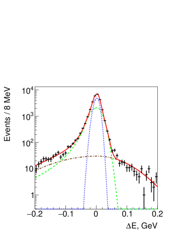
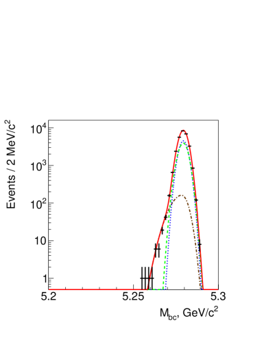
Figure 1: Projections of the resolution fit results onto $\Delta E$ and $M_{\text{bc}}$ for the channel $B^{+}\to\eta_{c2}(1D)K^{+}$ with $\eta_{c}\to K^{+}K^{0}_{S}\pi^{-}$. The points with error bars are truth-matched signal MC, the red solid curve is the fit result, the green dashed curve is the Crystal Ball component, the blue dotted curve is the first Gaussian component, and the brown dash-dotted curve is the second Gaussian component.

4.3 Fit to the $(\Delta E,M_{\text{bc}})$ distribution

The $(\Delta E,M_{\text{bc}})$ distribution is fitted in order to determine the expected number of the background events in the signal region. The distribution is fitted using the function

$$N_{S}S(\Delta E,M_{\text{bc}})+B(\Delta E,M_{\text{bc}}),$$ (5)

where $N_{S}$ is the number of signal events and $B$ is the background density function that is given by

$$B(\Delta E,M_{\text{bc}})=\sqrt{m_{0}-M_{\text{bc}}}\exp[-a(m_{0}-M_{\text{bc}})]P_{3}(\Delta E,M_{\text{bc}}),$$ (6)

where $m_{0}$ is the threshold mass, $a$ is a rate parameter and $P_{3}$ is a two-dimensional third-order polynomial. Example $(\Delta E,M_{\text{bc}})$ fit results (for the channel $B^{+}\to\eta_{c2}(1D)K^{+}$ with $\eta_{c}\to K^{+}K^{0}_{S}\pi^{-}$) are shown in figure 2.

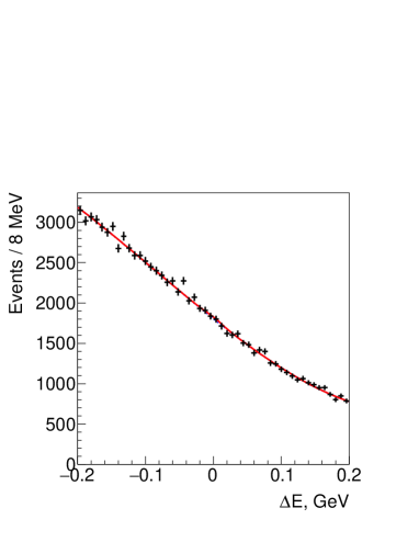
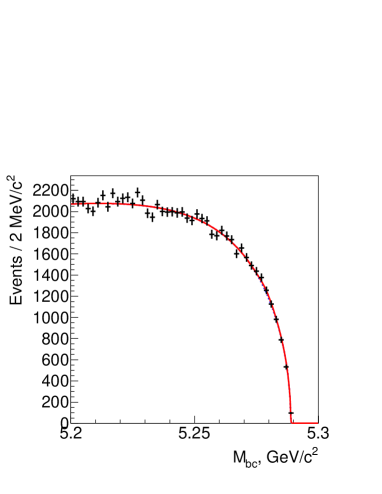
Figure 2: Projections of the results of the fit to the $(\Delta E,M_{\text{bc}})$ distribution onto $\Delta E$ (with $M_{\text{bc}}>5.272\ \text{GeV}/c^{2}$) and $M_{\text{bc}}$ (with $|\Delta E|<20\ \text{MeV}$) for the channel $B^{+}\to\eta_{c2}(1D)K^{+}$ with $\eta_{c}\to K^{+}K^{0}_{S}\pi^{-}$. The points with error bars are data, the red solid curve is the fit result, and the blue dotted curve is the background. Since there is no significant signal before the optimization of the selection requirements and for the entire $\eta_{c}\gamma$ mass range, the two curves almost coincide.

4.4 Multivariate analysis

To improve the separation of signal and background events, a multivariate analysis is performed for each individual $\eta_{c}$ decay channel. As in ref. Chilikin:2019wzy , the multivariate analysis is performed using the multilayer perceptron (MLP) neural network implemented in the tmva library tmva . However, the details of the procedure depend on the particular $B$ decay mode and, consequently, differ from ref. Chilikin:2019wzy .

The following variables are always included in the neural network: the angle between the thrust axes of the $B$ candidate and the remaining particles in the event, the angle between the thrust axes of all tracks and all photons in the event, the ratio of the Fox-Wolfram moments $F_{2}/F_{0}$, the $B$ production angle ($\Upsilon(4S)$ helicity angle), the quality of the vertex fit of all $B$ daughter tracks, $K^{0}_{S}$, and $\Lambda$ to a common vertex, the $h_{c}$ and $\eta_{c}$ masses, and the maximal $\pi^{0}$ likelihoods for the $\eta_{c2}(1D)$ and $h_{c}$ daughter photons combined with any other photon in the event. The $\pi^{0}$ likelihood is based on the energy and the polar angle of the transition-photon candidate in the laboratory frame and the $\pi^{0}$ invariant mass. Note that the ratio of the Fox-Wolfram moments is already required to be less than 0.3 at the event-selection stage. This requirement does not significantly modify the final selection results, because the rejection of background with $F_{2}/F_{0}>0.3$ can also be performed by the MLP. However, it lowers the fraction of the background that needs to be rejected by the MLP, which is helpful to reduce overtraining.

For the decays $B^{+}\to\eta_{c2}(1D)K^{+}$ and $B^{0}\to\eta_{c2}(1D)K^{0}_{S}$, the MLP also includes the $\eta_{c2}(1D)$ helicity angle and the $h_{c}$ daughter-photon azimuthal angle for every $\eta_{c}$ channel. The $\eta_{c2}(1D)$ helicity angle is defined as the angle between $-\vec{p}_{K}$ and $\vec{p}_{h_{c}}$, where $\vec{p}_{K}$ and $\vec{p}_{h_{c}}$ are the momenta of $K$ and $h_{c}$ in the $\eta_{c2}(1D)$ rest frame, respectively. The azimuthal angle of the $h_{c}$ daughter photon is defined as the angle between the planes of the $h_{c}$ and $\eta_{c2}(1D)$ daughter-photon momenta and the momenta of the $\eta_{c2}(1D)$ daughter photon and $K^{+}$ or $K^{0}_{S}$ in the $h_{c}$ rest frame. The definition is shown in figure 3.

Figure 3: Definition of the azimuthal angle $\varphi_{\gamma_{2}}$ of the $h_{c}$ daughter photon (in the $h_{c}$ rest frame). The $\eta_{c2}(1D)$ daughter photon is denoted as $\gamma_{1}$.

For the channels $\eta_{c}\to K^{+}K^{0}_{S}\pi^{-}$, $\eta_{c}\to K^{+}K^{-}\pi^{0}$, and $\eta_{c}\to K^{0}_{S}K^{0}_{S}\pi^{0}$, two invariant masses of the $\eta_{c}$ daughter particle pairs (both $K\pi$ combinations) are included in the neural network.

The following particle identification variables are included into the neural network if there are corresponding charged particles in the final state: the minimum likelihood ratio $R_{K/\pi}$ of the $\eta_{c}$ daughter kaons, the minimum of the two likelihood ratios $R_{p/K}$, $R_{p/\pi}$ of the $\eta_{c}$ daughter protons, and $R_{K/\pi}$ for the daughter $K^{+}$ of the $B$ meson (for the decays $B^{+}\to\eta_{c2}(1D)K^{+}$ and $B^{0}\to\eta_{c2}(1D)\pi^{-}K^{+}$).

If there is a $\pi^{0}$ or $\eta$ in the final state, four additional variables are included: the $\pi^{0}$ ($\eta$) mass, the minimal energy of the $\pi^{0}$ ($\eta$) daughter photons in the laboratory frame, and the number of $\pi^{0}$ candidates that include a $\pi^{0}$ ($\eta$) daughter photon as one of their daughters (for each of the $\pi^{0}$ ($\eta$) daughter photons). If the $\eta_{c}$ has an $\eta^{\prime}$ daughter, then the mass of the $\eta^{\prime}$ candidate is also included in the neural network.

The training and testing signal samples are taken from the signal MC. The background sample is taken from a two-dimensional $(\Delta E,M_{\text{bc}})$ sideband defined as all selected events outside the signal region defined by eq. 1. The background sample is divided into training and testing samples.

4.5 Global optimization of the selection requirements

The global selection-requirement optimization is performed by maximizing the value

$$F_{\text{opt}}=\frac{\sum\limits_{i}N_{\text{sig}}^{(i)}}{\displaystyle{\frac{a}{2}}+\sqrt{\sum\limits_{i}N_{\text{bg}}^{(i)}}},$$ (7)

where $i$ is the channel index, $N_{\text{sig}}^{(i)}$ and $N_{\text{bg}}^{(i)}$ are the expected numbers of the signal and background events for the $i$-th channel in the signal region, respectively, and $a=3$ is the target significance. This optimization method is based on ref. Punzi:2003bu .

The signal region is defined as

$$\left(\frac{\Delta E}{R_{\Delta E}^{(i)}}\right)^{2}+\left(\frac{M_{\text{bc}}-m_{B}}{R_{M_{\text{bc}}}^{(i)}}\right)^{2}<1.$$ (8)

where $R_{\Delta E}^{(i)}$ and $R_{M_{\text{bc}}}^{(i)}$ are the half-axes of the signal region ellipse. The parameters determined by the optimization are $R_{\Delta E}^{(i)}$, $R_{M_{\text{bc}}}^{(i)}$, and the minimal value of the MLP output ($v_{0}^{(i)}$) for each channel.

The expected number of signal events for $B^{+}\to\eta_{c2}(1D)K^{+}$ is calculated as

$$N_{\text{sig}}^{(i)}= 2N_{\Upsilon(4S)}\mathcal{B}(\Upsilon(4S)\to B^{+}B^{-})\mathcal{B}(B^{+}\to\eta_{c2}(1D)K^{+})\mathcal{B}(\eta_{c2}(1D)\to h_{c}\gamma)$$ (9)

$$\times\mathcal{B}(h_{c}\to\eta_{c}\gamma)\mathcal{B}(\eta_{c}\to i)\epsilon_{\text{SR}}^{(i)}\epsilon_{S}^{(i)}(v_{0}^{(i)}),$$

where $N_{\Upsilon(4S)}$ is the number of $\Upsilon(4S)$ events, $\mathcal{B}(\eta_{c}\to i)$ is the branching fraction of the $\eta_{c}$ decay to its $i$-th decay channel, $\epsilon_{\text{SR}}^{(i)}$ is the reconstruction efficiency for the specific signal region SR before the requirement ($v>v_{0}^{(i)}$) on the MLP output variable $v$ for the signal events, and $\epsilon_{S}^{(i)}(v_{0}^{(i)})$ is the efficiency of the MLP-output requirement. The number of $\Upsilon(4S)$ events is assumed to be equal to the number of $B\bar{B}$ pairs; the branching fraction $\mathcal{B}(\Upsilon(4S)\to B^{+}B^{-})$ is calculated under the same assumption in ref. Tanabashi:2018oca . The signal-region-dependent reconstruction efficiency is calculated as

$$\epsilon_{\text{SR}}^{(i)}=\epsilon_{R}^{(i)}\int\limits_{\text{SR}}S_{i}(\Delta E,M_{\text{bc}})d\Delta EdM_{\text{bc}},$$ (10)

where $\epsilon_{R}^{(i)}$ is the reconstruction efficiency, and $S_{i}$ is the signal probability density function for $i$-th $\eta_{c}$ decay channel (the integral of $S_{i}$ over the signal region is the efficiency of the signal region selection). The unknown branching-fraction product $\mathcal{B}(B^{+}\to\eta_{c2}(1D)K^{+})\times\mathcal{B}(\eta_{c2}(1D)\to h_{c}\gamma)$ can be set to an arbitrary value because the maximum of $F_{\text{opt}}$ does not depend on it. The expected number of signal events for $B^{0}\to\eta_{c2}(1D)K^{0}_{S}$ is calculated in a similar manner.

The expected number of background events is calculated as

$$N_{\text{bg}}^{(i)}=\epsilon_{B}^{(i)}(v_{0}^{(i)})\frac{N_{\eta_{c2}(1D)\text{ region}}}{N_{\text{full}}}\int\limits_{\text{SR}}B_{i}(\Delta E,M_{\text{bc}})d\Delta EdM_{\text{bc}},$$ (11)

where $\epsilon_{B}^{(i)}(v_{0}^{(i)})$ is the efficiency of the MLP output requirement for the background events, $N_{\eta_{c2}(1D)\text{ region}}$ is the number of background events in the $\eta_{c2}(1D)$ region defined by eq. (2), $N_{\text{full}}$ is the full number of background events, and $B_{i}$ is the background density function.

The results are shown in table 1 for the decay $B^{+}\to\eta_{c2}(1D)K^{+}$, in table 2 for the decay $B^{0}\to\eta_{c2}(1D)K^{0}_{S}$, in table 3 for the combination of $B^{+}\to\eta_{c2}(1D)K^{+}$ and $B^{0}\to\eta_{c2}(1D)K^{0}_{S}$, in table 4 for the decay $B^{0}\to\eta_{c2}(1D)\pi^{-}K^{+}$, and in table 5 for the decay $B^{+}\to\eta_{c2}(1D)\pi^{+}K^{0}_{S}$. To combine the decays $B^{+}\to\eta_{c2}(1D)K^{+}$ and $B^{0}\to\eta_{c2}(1D)K^{0}_{S}$, a separate optimization that includes all combinations of $B$ and $\eta_{c}$ channels is performed. To estimate the expected number of signal events in the combined sample, the partial widths of the decays $B^{+}\to\eta_{c2}(1D)K^{+}$ and $B^{0}\to\eta_{c2}(1D)K^{0}$ are assumed to be the same.

Table 1: Results of the optimization of the selection requirements for the channel $B^{+}\to\eta_{c2}(1D)K^{+}$. The expected number of signal events is calculated assuming $\mathcal{B}(B^{+}\to\eta_{c2}(1D)K^{+})\times\mathcal{B}(\eta_{c2}(1D)\to h_{c}\gamma)=1.0\times 10^{-5}$. The efficiencies and expected numbers of signal and background events are calculated for the training sample. The signal-region half-axes $R_{\Delta E}^{(i)}$ ($R_{M_{\text{bc}}}^{(i)}$) are in MeV ($\text{MeV}/c^{2}$); all other values are dimensionless.

Channel	Parameters		Efficiency			Events
	$R_{\Delta E}^{(i)}$	$R_{M_{\text{bc}}}^{(i)}$	$\epsilon_{\text{SR}}^{(i)}$	$\epsilon_{S}^{(i)}(v_{0}^{(i)})$	$\epsilon_{B}^{(i)}(v_{0}^{(i)})$	$N_{\text{sig}}^{(i)}$	$N_{\text{bg}}^{(i)}$
$K^{+}K^{0}_{S}\pi^{-}$	23.3	4.85	4.29%	51.3%	2.22%	2.16	9.82
$K^{+}K^{-}\pi^{0}$	18.4	4.11	2.76%	32.8%	0.37%	0.44	2.82
$K^{0}_{S}K^{0}_{S}\pi^{0}$	18.0	3.80	0.93%	21.5%	0.20%	0.02	0.17
$K^{+}K^{-}\eta$	21.5	4.70	2.93%	15.2%	0.07%	0.05	0.26
$K^{+}K^{-}K^{+}K^{-}$	20.0	4.33	3.47%	42.1%	1.97%	0.09	0.49
$\eta^{\prime}(\to\eta\pi^{+}\pi^{-})\pi^{+}\pi^{-}$	21.3	4.64	2.02%	24.1%	0.13%	0.09	0.47
$p\bar{p}$	30.1	5.61	12.53%	66.4%	4.50%	0.51	1.52
$p\bar{p}\pi^{0}$	19.5	4.24	3.36%	21.1%	0.16%	0.10	0.62
$p\bar{p}\pi^{+}\pi^{-}$	18.0	3.99	4.13%	21.1%	0.46%	0.19	1.18
$\Lambda\bar{\Lambda}$	30.4	5.67	2.71%	59.9%	3.16%	0.07	0.22

Table 2: Results of the optimization of the selection requirements for the channel $B^{0}\to\eta_{c2}(1D)K^{0}_{S}$. The expected number of signal events is calculated assuming $\mathcal{B}(B^{+}\to\eta_{c2}(1D)K^{+})\times\mathcal{B}(\eta_{c2}(1D)\to h_{c}\gamma)=1.0\times 10^{-5}$ and equal partial widths of the decays $B^{+}\to\eta_{c2}(1D)K^{+}$ and $B^{0}\to\eta_{c2}(1D)K^{0}$. The efficiencies and expected numbers of signal and background events are calculated for the training sample. The signal-region half-axes $R_{\Delta E}^{(i)}$ ($R_{M_{\text{bc}}}^{(i)}$) are in MeV ($\text{MeV}/c^{2}$); all other values are dimensionless.

Channel	Parameters		Efficiency			Events
	$R_{\Delta E}^{(i)}$	$R_{M_{\text{bc}}}^{(i)}$	$\epsilon_{\text{SR}}^{(i)}$	$\epsilon_{S}^{(i)}(v_{0}^{(i)})$	$\epsilon_{B}^{(i)}(v_{0}^{(i)})$	$N_{\text{sig}}^{(i)}$	$N_{\text{bg}}^{(i)}$
$K^{+}K^{0}_{S}\pi^{-}$	24.5	5.06	2.75%	61.2%	4.27%	0.73	4.88
$K^{+}K^{-}\pi^{0}$	19.2	4.12	1.77%	45.8%	1.09%	0.17	1.85
$K^{0}_{S}K^{0}_{S}\pi^{0}$	17.0	3.51	0.51%	33.5%	0.61%	0.01	0.12
$K^{+}K^{-}\eta$	20.0	4.43	1.72%	25.7%	0.29%	0.02	0.21
$K^{+}K^{-}K^{+}K^{-}$	22.5	4.73	2.24%	49.6%	3.06%	0.03	0.22
$\eta^{\prime}(\to\eta\pi^{+}\pi^{-})\pi^{+}\pi^{-}$	21.9	4.64	1.21%	32.7%	0.32%	0.03	0.29
$p\bar{p}$	34.7	6.06	8.23%	70.6%	6.73%	0.16	0.65
$p\bar{p}\pi^{0}$	19.5	4.29	2.08%	26.8%	0.34%	0.04	0.36
$p\bar{p}\pi^{+}\pi^{-}$	19.9	4.27	2.71%	30.1%	0.92%	0.08	0.74
$\Lambda\bar{\Lambda}$	34.0	6.06	1.71%	65.1%	4.66%	0.02	0.09

Table 3: Results of the optimization of the selection requirements for the combination of the channels $B^{+}\to\eta_{c2}(1D)K^{+}$ and $B^{0}\to\eta_{c2}(1D)K^{0}_{S}$. The expected number of signal events is calculated assuming $\mathcal{B}(B^{+}\to\eta_{c2}(1D)K^{+})\times\mathcal{B}(\eta_{c2}(1D)\to h_{c}\gamma)=1.0\times 10^{-5}$ and equal partial widths of the decays $B^{+}\to\eta_{c2}(1D)K^{+}$ and $B^{0}\to\eta_{c2}(1D)K^{0}$. The efficiencies and expected numbers of signal and background events are calculated for the training sample. The signal-region half-axes $R_{\Delta E}^{(i)}$ ($R_{M_{\text{bc}}}^{(i)}$) are in MeV ($\text{MeV}/c^{2}$); all other values are dimensionless.

Channel	Parameters		Efficiency			Events
	$R_{\Delta E}^{(i)}$	$R_{M_{\text{bc}}}^{(i)}$	$\epsilon_{\text{SR}}^{(i)}$	$\epsilon_{S}^{(i)}(v_{0}^{(i)})$	$\epsilon_{B}^{(i)}(v_{0}^{(i)})$	$N_{\text{sig}}^{(i)}$	$N_{\text{bg}}^{(i)}$
$B^{+}\to\eta_{c2}(1D)K^{+}$
$K^{+}K^{0}_{S}\pi^{-}$	24.3	4.93	4.37%	45.3%	1.55%	1.95	7.27
$K^{+}K^{-}\pi^{0}$	17.0	3.90	2.58%	32.8%	0.37%	0.41	2.48
$K^{0}_{S}K^{0}_{S}\pi^{0}$	16.8	3.52	0.86%	21.5%	0.20%	0.02	0.15
$K^{+}K^{-}\eta$	20.4	4.45	2.80%	15.2%	0.07%	0.05	0.23
$K^{+}K^{-}K^{+}K^{-}$	20.8	4.49	3.58%	34.3%	1.25%	0.07	0.33
$\eta^{\prime}(\to\eta\pi^{+}\pi^{-})\pi^{+}\pi^{-}$	20.2	4.47	1.94%	24.1%	0.13%	0.09	0.43
$p\bar{p}$	28.4	5.48	12.27%	66.4%	4.50%	0.50	1.40
$p\bar{p}\pi^{0}$	18.4	4.04	3.19%	20.8%	0.16%	0.10	0.54
$p\bar{p}\pi^{+}\pi^{-}$	16.7	3.83	3.88%	20.9%	0.45%	0.17	1.04
$\Lambda\bar{\Lambda}$	28.8	5.55	2.66%	59.9%	3.16%	0.07	0.20
$B^{0}\to\eta_{c2}(1D)K^{0}_{S}$
$K^{+}K^{0}_{S}\pi^{-}$	24.8	4.92	2.73%	44.9%	1.71%	0.53	1.91
$K^{+}K^{-}\pi^{0}$	17.6	3.87	1.64%	28.3%	0.40%	0.10	0.59
$K^{0}_{S}K^{0}_{S}\pi^{0}$	16.1	3.43	0.49%	9.0%	0.09%	0.00	0.02
$K^{+}K^{-}\eta$	14.0	3.17	1.17%	25.7%	0.29%	0.01	0.11
$K^{+}K^{-}K^{+}K^{-}$	19.2	4.18	2.00%	41.5%	2.04%	0.02	0.11
$\eta^{\prime}(\to\eta\pi^{+}\pi^{-})\pi^{+}\pi^{-}$	19.8	4.28	1.12%	24.7%	0.16%	0.02	0.12
$p\bar{p}$	32.7	5.57	8.00%	65.4%	4.57%	0.14	0.38
$p\bar{p}\pi^{0}$	16.0	3.62	1.72%	18.8%	0.18%	0.02	0.13
$p\bar{p}\pi^{+}\pi^{-}$	16.7	3.74	2.33%	22.8%	0.52%	0.05	0.30
$\Lambda\bar{\Lambda}$	35.5	6.15	1.73%	54.9%	1.78%	0.02	0.04

Table 4: Results of the optimization of the selection requirements for the channel $B^{0}\to\eta_{c2}(1D)\pi^{-}K^{+}$. The expected number of signal events is calculated assuming $\mathcal{B}(B^{0}\to\eta_{c2}(1D)\pi^{-}K^{+})\times\mathcal{B}(\eta_{c2}(1D)\to h_{c}\gamma)=1.0\times 10^{-5}$. The efficiencies and expected numbers of signal and background events are calculated for the training sample. The signal-region half-axes $R_{\Delta E}^{(i)}$ ($R_{M_{\text{bc}}}^{(i)}$) are in MeV ($\text{MeV}/c^{2}$); all other values are dimensionless.

Channel	Parameters		Efficiency			Events
	$R_{\Delta E}^{(i)}$	$R_{M_{\text{bc}}}^{(i)}$	$\epsilon_{\text{SR}}^{(i)}$	$\epsilon_{S}^{(i)}(v_{0}^{(i)})$	$\epsilon_{B}^{(i)}(v_{0}^{(i)})$	$N_{\text{sig}}^{(i)}$	$N_{\text{bg}}^{(i)}$
$K^{+}K^{0}_{S}\pi^{-}$	20.1	4.54	2.91%	40.3%	1.45%	1.09	33.26
$K^{+}K^{-}\pi^{0}$	15.6	3.64	1.83%	24.9%	0.26%	0.21	9.29
$K^{0}_{S}K^{0}_{S}\pi^{0}$	12.1	2.87	0.43%	20.3%	0.21%	0.01	0.56
$K^{+}K^{-}\eta$	13.6	3.32	1.44%	16.7%	0.11%	0.02	1.22
$K^{+}K^{-}K^{+}K^{-}$	16.8	3.92	2.22%	23.2%	0.61%	0.03	1.14
$\eta^{\prime}(\to\eta\pi^{+}\pi^{-})\pi^{+}\pi^{-}$	17.3	3.92	1.18%	20.7%	0.10%	0.04	1.75
$p\bar{p}$	25.0	5.23	9.01%	61.9%	5.24%	0.32	7.10
$p\bar{p}\pi^{0}$	14.4	3.48	1.97%	16.8%	0.14%	0.04	2.09
$p\bar{p}\pi^{+}\pi^{-}$	16.3	3.81	2.74%	9.8%	0.12%	0.05	2.23
$\Lambda\bar{\Lambda}$	24.8	5.23	1.82%	54.9%	3.48%	0.04	0.94

Table 5: Results of the optimization of the selection requirements for the channel $B^{+}\to\eta_{c2}(1D)\pi^{+}K^{0}_{S}$. The expected number of signal events is calculated assuming $\mathcal{B}(B^{0}\to\eta_{c2}(1D)\pi^{-}K^{+})\times\mathcal{B}(\eta_{c2}(1D)\to h_{c}\gamma)=1.0\times 10^{-5}$ and equal partial widths of the decays $B^{0}\to\eta_{c2}(1D)\pi^{-}K^{+}$ and $B^{+}\to\eta_{c2}(1D)\pi^{+}K^{0}$. The efficiencies and expected numbers of signal and background events are calculated for the training sample. The signal-region half-axes $R_{\Delta E}^{(i)}$ ($R_{M_{\text{bc}}}^{(i)}$) are in MeV ($\text{MeV}/c^{2}$); all other values are dimensionless.

Channel	Parameters		Efficiency			Events
	$R_{\Delta E}^{(i)}$	$R_{M_{\text{bc}}}^{(i)}$	$\epsilon_{\text{SR}}^{(i)}$	$\epsilon_{S}^{(i)}(v_{0}^{(i)})$	$\epsilon_{B}^{(i)}(v_{0}^{(i)})$	$N_{\text{sig}}^{(i)}$	$N_{\text{bg}}^{(i)}$
$K^{+}K^{0}_{S}\pi^{-}$	21.6	4.69	1.64%	40.0%	1.64%	0.299	16.82
$K^{+}K^{-}\pi^{0}$	15.6	3.57	0.94%	22.1%	0.33%	0.047	4.29
$K^{0}_{S}K^{0}_{S}\pi^{0}$	12.4	2.82	0.24%	11.1%	0.14%	0.002	0.17
$K^{+}K^{-}\eta$	15.8	3.67	0.90%	16.4%	0.12%	0.007	0.66
$K^{+}K^{-}K^{+}K^{-}$	17.9	4.11	1.24%	27.3%	0.85%	0.009	0.67
$\eta^{\prime}(\to\eta\pi^{+}\pi^{-})\pi^{+}\pi^{-}$	12.9	3.01	0.45%	21.3%	0.21%	0.008	0.85
$p\bar{p}$	27.4	5.39	5.06%	61.3%	5.40%	0.089	3.61
$p\bar{p}\pi^{0}$	16.1	3.67	1.14%	13.3%	0.11%	0.010	0.88
$p\bar{p}\pi^{+}\pi^{-}$	16.3	3.88	1.46%	11.9%	0.17%	0.017	1.39
$\Lambda\bar{\Lambda}$	26.1	5.36	0.99%	50.2%	3.42%	0.010	0.44

5 Fit to the data

5.1 Fit results in the default model

After the global optimization of the selection requirements, the selected events are merged into a single data sample. The best-candidate selection is performed for each $\eta_{c}$ channel separately by using the maximal MLP output value; the selection procedure is the same as in ref. Chilikin:2019wzy . The fraction of removed candidates is 10% to 23%, depending on the $\eta_{c}$ channel, for the two-body decays $B^{+}\to\eta_{c2}(1D)K^{+}$ and $B^{0}\to\eta_{c2}(1D)K^{0}_{S}$; for the three-body decays $B^{0}\to\eta_{c2}(1D)\pi^{-}K^{+}$ and $B^{+}\to\eta_{c2}(1D)\pi^{+}K^{0}_{S}$, the fraction is (21-42)%. Multiple candidates originating from different $\eta_{c}$ decay channels are allowed, however, no events with multiple candidates are observed in the signal region for any of the signal $B$ decays.

We perform an extended unbinned maximum likelihood fit to the data in the signal region. The $\eta_{c2}(1D)$ is represented by the Breit-Wigner amplitude:

$$A_{\eta_{c2}(1D)}(M_{\eta_{c2}(1D)})=\frac{1}{m_{\eta_{c2}(1D)}^{2}-M_{\eta_{c2}(1D)}^{2}-iM_{\eta_{c2}(1D)}\Gamma_{\eta_{c2}(1D)}},$$ (12)

where $\Gamma_{\eta_{c2}(1D)}$ is the $\eta_{c2}(1D)$ width. Since the $\eta_{c2}(1D)$ is expected to be narrower than the resolution, it is sufficient to use the constant-width parameterization given by eq. (12). The $M_{h_{c}\gamma}$ distribution is fitted to the function

$$S(M)=\left(N_{\eta_{c2}(1D)}|A_{\eta_{c2}(1D)}(M)|^{2}\right)\otimes R_{\eta_{c2}(1D)}(M)+P_{2}(M),$$ (13)

where $N_{\eta_{c2}(1D)}$ is the number of signal events, $R_{\eta_{c2}(1D)}(M)$ is the $\eta_{c2}(1D)$ mass resolution that is determined from MC and parameterized as a sum of two asymmetric Gaussians, and $P_{2}$ is a second-order polynomial representing the background shape. For the channel $B^{0}\to\eta_{c2}(1D)K^{0}_{S}$, that has the lowest number of events, the default order of the background polynomial is reduced to 1. The $\eta_{c2}(1D)$ width is fixed at $500\ \text{keV}$. The chosen default width value is approximately equal to the sum of individual partial widths predicted in ref. Eichten:2002qv : $\Gamma(\eta_{c2}(1D)\to h_{c}\gamma)+\Gamma(\eta_{c2}(1D)\to gg)+\Gamma(\eta_{c2}(1D)\to\eta_{c}\pi\pi)=458\ \text{keV}$. Another prediction of the $\eta_{c2}(1D)$ width was made in ref. Fan:2009cj ; it is estimated to be within the range from $660$ to $810\ \text{keV}$. The variation of the $\eta_{c2}(1D)$ width is considered as a source of systematic uncertainty.

The fit results corresponding to the most significant peaks within the $\eta_{c2}(1D)$ search region are shown in figure 4 for the decays $B^{+}\to\eta_{c2}(1D)K^{+}$ and $B^{0}\to\eta_{c2}(1D)K^{0}_{S}$, in figure 5 for their combination, and in figure 6 for the decays $B^{0}\to\eta_{c2}(1D)\pi^{-}K^{+}$ and $B^{+}\to\eta_{c2}(1D)\pi^{+}K^{0}_{S}$. The masses, yields, and local significances of the most significant peaks within the search region are listed in table 6. The local significances are calculated from the difference of $(-2\ln L)$ assuming that the mass is known (with one degree of freedom). There is no significant signal in any channel; since even the local significance does not exceed $3\sigma$, the global significance is not calculated.

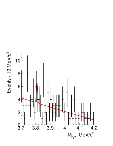
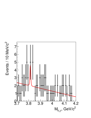
Figure 4: Fit results for the channels $B^{+}\to\eta_{c2}(1D)K^{+}$ (left) and $B^{0}\to\eta_{c2}(1D)K^{0}_{S}$ (right).

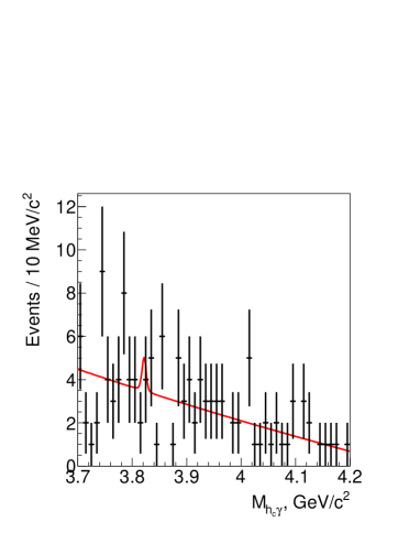
Figure 5: Fit results for the combination of channels $B^{+}\to\eta_{c2}(1D)K^{+}$ and $B^{0}\to\eta_{c2}(1D)K^{0}_{S}$.

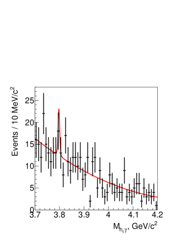
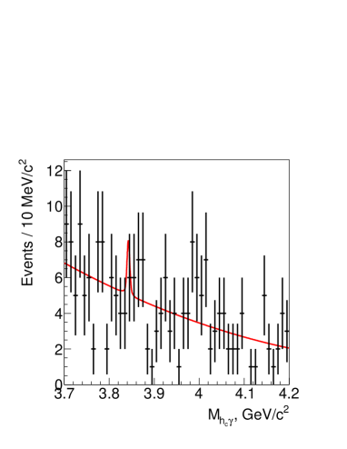
Figure 6: Fit results for the channels $B^{0}\to\eta_{c2}(1D)\pi^{-}K^{+}$ (left) and $B^{+}\to\eta_{c2}(1D)\pi^{+}K^{0}_{S}$ (right).

Table 6: The masses, yields, and local significances of the most significant peaks within the search region.

Channel	Mass, $\text{MeV}/c^{2}$	Yield	Local significance
$B^{+}\to\eta_{c2}(1D)K^{+}$	$3809.6\pm 4.3$	$3.3\pm 3.0$	$1.3\sigma$
$B^{0}\to\eta_{c2}(1D)K^{0}_{S}$	$3814.4\pm 2.7$	$2.7\pm 2.3$	$1.5\sigma$
$B^{+}\to\eta_{c2}(1D)K^{+}$ and $B^{0}\to\eta_{c2}(1D)K^{0}_{S}$	$3821.8\pm 4.4$	$1.6\pm 3.2$	$0.7\sigma$
$B^{0}\to\eta_{c2}(1D)\pi^{-}K^{+}$	$3797.0\pm 1.6$	$9.4\pm 5.1$	$2.1\sigma$
$B^{+}\to\eta_{c2}(1D)\pi^{+}K^{0}_{S}$	$3842.3\pm 3.4$	$2.6\pm 3.1$	$1.0\sigma$

5.2 Systematic uncertainties

The systematic errors in the branching-fraction products can be subdivided into three categories: branching-fraction scale errors, resolution errors, and model errors.

The sources of the systematic uncertainty in the branching-fraction scale include overtraining (the difference between the efficiency in the training and testing samples), the error on the difference of the particle-identification requirement efficiency between the data and MC, the tracking efficiency error, the difference between the MLP efficiency for data and MC, the unknown amplitude of the $B^{0}\to\eta_{c2}(1D)\pi^{-}K^{+}$ and $B^{+}\to\eta_{c2}(1D)\pi^{+}K^{0}_{S}$ decays, the number of $\Upsilon(4S)$ events, and the $\eta_{c}$, $h_{c}$, and $\Upsilon(4S)$ branching fractions.

The difference of the particle-identification requirement efficiency between the data and MC is estimated from several control samples, including $D^{*+}\to D^{0}(\to K^{-}\pi^{+})\pi^{+}$ for $K$ and $\pi$, $\Lambda\to p\pi^{-}$ for $p$, $\Lambda_{c}^{+}\to\Lambda\pi^{+}$ for $\Lambda$, $D^{0}\to K^{0}_{S}\pi^{+}\pi^{-}$ for $K^{0}_{S}$, and $\tau^{-}\to\pi^{-}\pi^{0}\nu_{\tau}$ for $\pi^{0}$ candidates, respectively.

The uncertainty due to the difference in the MLP efficiency between the data and MC is estimated using the decay mode $B^{0}\to\eta_{c}\pi^{-}K^{+}$. This decay is reconstructed using selection criteria that are as similar as possible to the signal mode $B^{+}\to\eta_{c2}(1D)K^{+}$. The MLP optimized for $B^{+}\to\eta_{c2}(1D)K^{+}$ is applied to the control channel. Some MLP input variables used for the signal channel are undefined for $B^{0}\to\eta_{c}\pi^{-}K^{+}$, for example, the $\pi^{0}$ likelihood for photons. Such variables are set to constants. The ratio of the number of signal candidates in all channels after the application of MLP selection and in the channel $\eta_{c}\to K^{+}K^{0}_{S}\pi^{-}$ before the application of MLP selection is extracted from a simultaneous fit to the $\eta_{c}$ mass distributions and compared to its value in MC. The control-channel events are weighted to reproduce the selection efficiencies in the signal channel. The resulting ratio of the number of $\eta_{c}$ candidates is $0.82\pm 0.10$, while the ratio in MC is $0.98$. The relative difference between the data and MC efficiency is 16.8% and the statistical error of its determination is 9.9%. The statistical error is also added in quadrature to the systematic uncertainty. The resulting uncertainty from the MLP selection efficiency difference in data and MC is 19.5%. Since only the channel $\eta_{c}\to K^{+}K^{0}_{S}\pi^{-}$ is used without the MLP selection, this error includes also the error of the branching fractions of other $\eta_{c}$ channels relative to the channel $\eta_{c}\to K^{+}K^{0}_{S}\pi^{-}$.

The MLP efficiency uncertainty does not include the uncertainty caused by the difference between the data and MC in the distributions of the variables that are not defined for the channel $B^{0}\to\eta_{c}\pi^{-}K^{+}$. There are six such variables: the $\eta_{c2}(1D)$ helicity angle, the $h_{c}$ daughter-photon azimuthal angle, the $h_{c}$ and $\eta_{c}$ masses, and the $\pi^{0}$ likelihoods of the $\eta_{c2}(1D)$ and $h_{c}$ daughter photons. The distributions of the angular variables are known assuming negligible contribution of higher multipole amplitudes. No additional systematic uncertainty for the difference of their distributions in data and MC is assigned.

The error due to the $\eta_{c}$ mass distribution uncertainty is estimated by varying the $\eta_{c}$ mass and width by $\pm 1\sigma$ and reweighting the selected MC events; the largest resulting efficiency difference is treated as the systematic uncertainty from the $\eta_{c}$ mass distribution. The $\eta_{c}$ width uncertainty is increased up to the difference of the $\eta_{c}$ input and measured widths in the channel $B^{0}\to\eta_{c}\pi^{-}K^{+}$ to take into account the possible difference of the resolution.

Since the $h_{c}$ has a daughter photon that is not included into any kinematic fits before the calculation of the $h_{c}$ mass, the uncertainty in the $h_{c}$ mass distribution is caused mostly by the difference of the resolution in the photon energy in data and MC. This uncertainty is estimated by varying the photon energy correction Tamponi:2015xzb by $\pm 1\sigma$, reconstructing the MC events again using the new correction, and calculating the difference between the resulting efficiencies.

The uncertainty associated with the photon $\pi^{0}$ likelihoods is estimated using the decay $B^{+}\to\psi(2S)(\to\chi_{c1}(\to J/\psi\gamma)\gamma)K^{+}$. A neural network consisting of only two likelihoods is used to select the events in data and MC. The number of $\psi(2S)$ events in the data is calculated from a fit to the $(\chi_{c1}\gamma)$ invariant mass both before and after the application of the MLP selection. The difference of the efficiencies in data and MC is found to be 4.6%.

The uncertainty related to the unknown amplitude of the $B^{0}\to\eta_{c2}(1D)\pi^{-}K^{+}$ and $B^{+}\to\eta_{c2}(1D)\pi^{+}K^{0}_{S}$ decays is estimated by considering several decay amplitudes. By default, the distribution is assumed to be uniform. As an alternative, the decay is assumed to proceed via the intermediate $K^{*}(892)$ resonance. Two possible $K^{*}(892)$ polarizations are considered: $\lambda_{K^{*}(892)}=\pm 1$ and $\lambda_{K^{*}(892)}=0$, where $\lambda_{K^{*}(892)}$ is the $K^{*}(892)$ helicity. The angular distribution of the $K^{*}(892)$ decay is given by $|d^{1}_{\lambda_{K^{*}(892)}\,0}(\theta_{K^{*}(892)})|^{2}$, where $d$ is the Wigner $d$-function, and $\theta_{K^{*}(892)}$ is the $K^{*}(892)$ helicity angle (the angle between $-\vec{p}_{\eta_{c2}(1D)}$ and $\vec{p}_{K}$, where $\vec{p}_{\eta_{c2}(1D)}$ and $\vec{p}_{K}$ are the momenta of the $\eta_{c2}(1D)$ and $K$ in the $K^{*}(892)$ rest frame, respectively). The maximal deviations of the efficiency for alternative amplitude models from the default one are considered as systematic uncertainty. The uncertainties are found to be 15.0% and 9.5% for $B^{0}\to\eta_{c2}(1D)\pi^{-}K^{+}$ and $B^{+}\to\eta_{c2}(1D)\pi^{+}K^{0}_{S}$, respectively.

All systematic errors related to the branching-fraction scale are listed in table 7. The errors of the tracking efficiency and the difference of the particle-identification requirement efficiency depend on the $h_{c}$ decay channel; the values presented in table 7 are weighted averages.

Table 7: The systematic uncertainties of the branching-fraction scale.

Error source	$\eta_{c2}(1D)K^{+}$	$\eta_{c2}(1D)K^{0}_{S}$	$\eta_{c2}(1D)\pi^{-}K^{+}$	$\eta_{c2}(1D)\pi^{-}K^{0}_{S}$
Overtraining	3.7%	4.2%	2.0%	3.4%
PID	4.2%	5.1%	5.0%	5.5%
Tracking	1.5%	1.9%	1.9%	2.2%
MLP efficiency	19.5%	19.5%	19.5%	19.5%
$\pi^{0}$ likelihoods	4.6%	4.6%	4.6%	4.6%
$\eta_{c}$ mass distribution	5.5%	5.3%	5.6%	5.6%
Photon energy resolution	2.5%	1.7%	2.7%	1.3%
Amplitude of $B\to\eta_{c2}(1D)\pi K$	—	—	15.0%	9.5%
Number of $\Upsilon(4S)$ events	1.4%	1.4%	1.4%	1.4%
$\mathcal{B}$ of $\eta_{c}$ and $h_{c}$	13.6%	13.6%	13.6%	13.6%
$\mathcal{B}(\Upsilon(4S)\to B\bar{B})$	1.2%	1.2%	1.2%	1.2%
Total	25.7%	25.9%	29.8%	27.6%

5.3 Branching fraction

Since no significant signal is observed, a mass scan is performed over the $\eta_{c2}(1D)$ search region with a step size of $0.5\ \text{MeV}/c^{2}$. The confidence intervals for the branching-fraction products are calculated at each point.

The resolution scaling coefficient $\mathcal{S}$ is measured by modifying the resolution function $R_{\eta_{c2}(1D)}$:

$$R_{\eta_{c2}(1D)}(\Delta M)\to\frac{1}{\mathcal{S}}R_{\eta_{c2}(1D)}\left(\frac{\Delta M}{\mathcal{S}}\right),$$ (14)

and similarly for other processes. The difference of the resolution in the data and MC is estimated using the decay $B\to\psi(2S)(\to\chi_{c1}(\to J/\psi\gamma)\gamma)K$. This decay has two radiative transitions similar to the signal processes. The selection of the control channel is performed using a similar neural network, which has the same photon-related variables as in the signal process. After the photon resolution correction, no significant difference is observed between the resolution in the $\chi_{c1}$ mass in data and MC. The $\chi_{c1}$ mass resolution scaling coefficient is found to be $(0.99\pm 0.18)$ from a fit to the $\chi_{c1}$ mass. However, the resolution in the $\psi(2S)$ mass in data is found to be worse than the resolution in MC. The resolution scaling coefficient determined from a fit to the $\chi_{c1}\gamma$ invariant mass distribution is $(1.31\pm 0.12)$.

Four resolution scaling coefficients are selected for analysis: the nominal resolution ($\mathcal{S}=1.00$), the scaling coefficient determined from $B\to\psi(2S)(\to\chi_{c1}(\to J/\psi\gamma)\gamma)K$ ($\mathcal{S}=1.31$), and the same result varied by $\pm 1\sigma$ ($\mathcal{S}=1.19$ and $\mathcal{S}=1.43$).

For each of the selected scaling coefficients, several signal models are considered. They include the default model, the model without the signal, the model with a higher-order (2 for $B^{0}\to\eta_{c2}(1D)K^{0}_{S}$ and 3 for other decays) background polynomial, a model with variations of the $M_{h_{c}\gamma}$ fitting region, and a model with alternative values of the $\eta_{c2}(1D)$ width ($\Gamma_{\eta_{c2}(1D)}=0\ \text{MeV}$ and $1\ \text{MeV}$).

The confidence intervals are calculated for each model taking the branching-fraction scale error into account. For the channel $B^{0}\to\eta_{c2}(1D)\pi^{-}K^{+}$, the yield and its error are determined from the fit. To take the systematic error into account, the Feldman-Cousins unified confidence intervals Feldman:1997qc for the branching-fraction distribution are used:

$$\mathcal{B} =N_{\eta_{c2}(1D)}k,$$ (15)

$$\sigma_{\mathcal{B}} =\sqrt{\sigma_{N_{\eta_{c2}(1D)}}^{2}k^{2}+N_{\eta_{c2}(1D)}^{2}(k\sigma_{\mathcal{B}}^{\text{(scale)}})^{2}+\sigma_{N_{\eta_{c2}(1D)}}^{2}(k\sigma_{\mathcal{B}}^{\text{(scale)}})^{2}},$$

where $\mathcal{B}$ and $\sigma_{\mathcal{B}}$ are the mean and variance of the branching-fraction distribution, respectively, $k$ is the ratio of the branching fraction and observed number of events, $\sigma_{N_{\eta_{c2}(1D)}}$ is the uncertainty in the $\eta_{c2}(1D)$ yield, and $\sigma_{\mathcal{B}}^{\text{(scale)}}$ is the relative branching-fraction scale error determined in section 5.2 (the total error from table 7). Since the $\eta_{c2}(1D)$ yield is determined from the fit, the model without the signal is excluded from the list of alternative models for $B^{0}\to\eta_{c2}(1D)\pi^{-}K^{+}$.

For other decays: $B^{+}\to\eta_{c2}(1D)K^{+}$, $B^{0}\to\eta_{c2}(1D)K^{0}_{S}$, and $B^{+}\to\eta_{c2}(1D)\pi^{+}K^{0}_{S}$, it is not possible to determine the yield at all masses from the fit, because the number of events is too small. There are gaps without any events, where the likelihood is a continuously increasing function of the signal yield for all allowed values of the yield (such values that the overall fitting function is positive). Thus, it is necessary to switch to event counting. The counting region is chosen to be within $\pm 1.5(\sigma_{1}+\sigma_{2})/2$ from the current value of mass, where $\sigma_{1}$ and $\sigma_{2}$ are the parameters of the narrow asymmetric Gaussian used in the resolution fit. The expected number of background events is determined from the fit. The profile-likelihood-based intervals described in ref. Rolke:2004mj are used. The confidence-interval calculation takes into account the branching-fraction scale error.

The results of the confidence-interval determination for all resolution scaling coefficients and signal models are merged. For a specific $M_{h_{c}\gamma}$, the minimal lower limit and the maximal upper limit are selected. The resulting confidence intervals are shown in figure 7 for the channels $B^{+}\to\eta_{c2}(1D)K^{+}$ and $B^{0}\to\eta_{c2}(1D)K^{0}_{S}$ and in figure 8 for the channels $B^{0}\to\eta_{c2}(1D)\pi^{-}K^{+}$ and $B^{+}\to\eta_{c2}(1D)\pi^{+}K^{0}_{S}$.

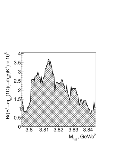
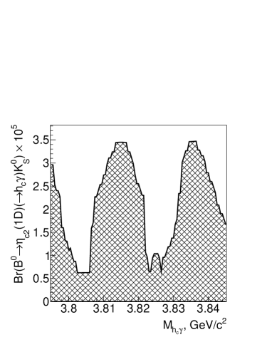
Figure 7: Confidence intervals (90% C. L.) for the branching-fraction products for the channels $B^{+}\to\eta_{c2}(1D)K^{+}$ (left) and $B^{0}\to\eta_{c2}(1D)K^{0}_{S}$ (right) including the systematic uncertainties.

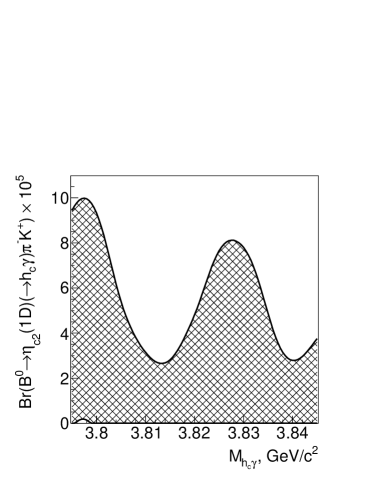
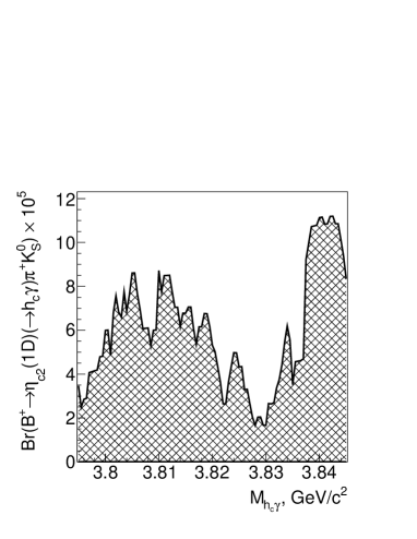
Figure 8: Confidence intervals (90% C. L.) for the branching-fraction products for the channels $B^{0}\to\eta_{c2}(1D)\pi^{-}K^{+}$ (left) and $B^{+}\to\eta_{c2}(1D)\pi^{+}K^{0}_{S}$ (right) including the systematic uncertainties.

6 Conclusions

A search for the $\eta_{c2}(1D)$ using the decays $B^{+}\to\eta_{c2}(1D)K^{+}$, $B^{0}\to\eta_{c2}(1D)K^{0}_{S}$, $B^{0}\to\eta_{c2}(1D)\pi^{-}K^{+}$ and $B^{+}\to\eta_{c2}(1D)\pi^{+}K^{0}_{S}$ has been carried out. No significant signal is found. Confidence intervals for branching fractions are determined in the $\eta_{c2}(1D)$ search range from 3795 to 3845 $\text{MeV}/c^{2}$. The scan results are shown in figure 7 and figure 8. The upper limits at 90% C. L. corresponding to $\eta_{c2}(1D)$ masses within the search range are

$$\mathcal{B}(B^{+}\to\eta_{c2}(1D)K^{+})\times\mathcal{B}(\eta_{c2}(1D)\to h_{c}\gamma) <3.7\times 10^{-5},$$

$$\mathcal{B}(B^{0}\to\eta_{c2}(1D)K^{0}_{S})\times\mathcal{B}(\eta_{c2}(1D)\to h_{c}\gamma) <3.5\times 10^{-5},$$

$$\mathcal{B}(B^{0}\to\eta_{c2}(1D)\pi^{-}K^{+})\times\mathcal{B}(\eta_{c2}(1D)\to h_{c}\gamma) <1.0\times 10^{-4},$$

$$\mathcal{B}(B^{+}\to\eta_{c2}(1D)\pi^{+}K^{0}_{S})\times\mathcal{B}(\eta_{c2}(1D)\to h_{c}\gamma) <1.1\times 10^{-4}.$$

The measured upper limit for $\mathcal{B}(B^{+}\to\eta_{c2}(1D)K^{+})\times\mathcal{B}(\eta_{c2}(1D)\to h_{c}\gamma)$ is consistent with the existing theoretical prediction of $(1.72\pm 0.42)\times 10^{-5}$ Xu:2016kbn . A data sample of about $10\ \text{ab}^{-1}$ is required to reach the expected value of branching-fraction product $\mathcal{B}(B^{+}\to\eta_{c2}(1D)K^{+})\times\mathcal{B}(\eta_{c2}(1D)\to h_{c}\gamma)\sim 1.0\times 10^{-5}$. Thus, the Belle II experiment should be able to observe the $\eta_{c2}(1D)$ or exclude the predicted branching fraction in the future Kou:2018nap .

References

- (1) P. A. Rapidis et al., Observation of a Resonance in Annihilation Just Above Charm Threshold, Phys. Rev. Lett. 39 (1977) 526, erratum: Phys. Rev. Lett. 39 (1977), 974.
- (2) S. Godfrey and N. Isgur, Mesons in a Relativized Quark Model with Chromodynamics, Phys. Rev. D 32 (1985) 189.
- (3) V. Bhardwaj et al. (Belle collaboration), Evidence of a new narrow resonance decaying to in , Phys. Rev. Lett. 111 (2013) 032001 [arXiv:1304.3975].
- (4) M. Ablikim et al. (BESIII Collaboration), Observation of the state in at BESIII, Phys. Rev. Lett. 115 (2015) 011803 [arXiv:1503.08203 [hep-ex]].
- (5) R. Aaij et al. (LHCb collaboration), Near-threshold spectroscopy and observation of a new charmonium state, JHEP 1907 (2019) 035 [arXiv:1903.12240].
- (6) L. P. Fulcher, Perturbative QCD, a universal QCD scale, long range spin orbit potential, and the properties of heavy quarkonia, Phys. Rev. D 44 (1991) 2079.
- (7) J. Zeng, J. W. Van Orden and W. Roberts, Heavy mesons in a relativistic model, Phys. Rev. D 52 (1995) 5229 [arXiv:hep-ph/9412269].
- (8) D. Ebert, R. N. Faustov and V. O. Galkin, Properties of heavy quarkonia and mesons in the relativistic quark model, Phys. Rev. D 67 (2003) 014027 [arXiv:hep-ph/0210381].
- (9) N. Brambilla et al. (Quarkonium Working Group), Heavy quarkonium physics, [arXiv:hep-ph/0412158].
- (10) D. Mohler, S. Prelovsek and R. M. Woloshyn, scattering and meson resonances from lattice QCD, Phys. Rev. D 87 (2013) 034501 [arXiv:1208.4059].
- (11) G. K. C. Cheung et al. (Hadron Spectrum collaboration), Excited and exotic charmonium, and meson spectra for two light quark masses from lattice QCD, JHEP 1612 (2016) 089 [arXiv:1610.01073].
- (12) E. J. Eichten, K. Lane and C. Quigg, B Meson Gateways to Missing Charmonium Levels, Phys. Rev. Lett. 89 (2002) 162002 [arXiv:hep-ph/0206018].
- (13) T. Barnes, S. Godfrey and E. S. Swanson, Higher charmonia, Phys. Rev. D 72 (2005) 054026 [arXiv:hep-ph/0505002].
- (14) Y. Fan, Z. G. He, Y. Q. Ma and K. T. Chao, Predictions of Light Hadronic Decays of Heavy Quarkonium 1D(2) States in NRQCD, Phys. Rev. D 80 (2009) 014001 [arXiv:0903.4572].
- (15) H. Xu, X. Liu and T. Matsuki, Understanding via rescattering mechanism and predicting , Phys. Rev. D 94 (2016) 034005 [arXiv:1605.04776].
- (16) K. Chilikin et al. (Belle Collaboration), Evidence for and observation of , Phys. Rev. D 100 (2019) 012001 [arXiv:1903.06414].
- (17) S. Kurokawa and E. Kikutani, Overview of the KEKB accelerators, Nucl. Instrum. Meth. A 499 (2003) 1.
- (18) T. Abe et al., Achievements of KEKB, PTEP 2013 (2013) 03A001.
- (19) A. Abashian et al. (Belle Collaboration), The Belle Detector, Nucl. Instrum. Meth. A 479 (2002) 117.
- (20) J. Brodzicka et al. (Belle Collaboration), Physics Achievements from the Belle Experiment, PTEP 2012 (2012) 04D001 [arXiv:1212.5342].
- (21) Z. Natkaniec et al., Status of the Belle silicon vertex detector, Nucl. Instrum. Meth. A 560 (2006) 1.
- (22) R. Brun, F. Bruyant, M. Maire, A. C. McPherson and P. Zanarini, Geant3, CERN-DD-EE-84-1.
- (23) D. J. Lange, The EvtGen particle decay simulation package, Nucl. Instrum. Methods Phys. Res., Sect. A 462 (2001) 152.
- (24) T. Kuhr et al. (Belle-II Framework Software Group), The Belle II Core Software, Comput. Softw. Big Sci. 3, (2019) 1 [arXiv:1809.04299].
- (25) M. Gelb et al., B2BII: Data Conversion from Belle to Belle II, Comput. Softw. Big Sci. 2 (2018) 9 [arXiv:1810.00019].
- (26) K. Hanagaki, H. Kakuno, H. Ikeda, T. Iijima and T. Tsukamoto, Electron identification in Belle, Nucl. Instrum. Methods Phys. Res., Sect. A 485 (2002) 490 [arXiv:hep-ex/0108044].
- (27) U. Tamponi et al. (Belle Collaboration), First observation of the hadronic transition and new measurement of the and parameters, Phys. Rev. Lett. 115 (2015) 142001 [arXiv:1506.08914].
- (28) M. Tanabashi et al. (Particle Data Group), Review of Particle Physics, Phys. Rev. D 98 (2018) 030001.
- (29) G. C. Fox and S. Wolfram, Observables for the Analysis of Event Shapes in e+ e- Annihilation and Other Processes, Phys. Rev. Lett. 41 (1978) 1581.
- (30) J. P. Lees et al. (BaBar Collaboration), Dalitz plot analysis of and in two-photon interactions, Phys. Rev. D 89 (2014) 112004 [arXiv:1403.7051].
- (31) T. Skwarnicki, A study of the radiative cascade transitions between the Upsilon-Prime and Upsilon resonances, DESY-F31-86-02.
- (32) H. Voss, A. Hocker, J. Stelzer and F. Tegenfeldt, TMVA - Toolkit for Multivariate Data Analysis, PoS ACAT (2007) 040 [arXiv:physics/0703039].
- (33) G. Punzi, Sensitivity of searches for new signals and its optimization, eConf C 030908 (2003) MODT002 [arXiv:physics/0308063].
- (34) G. J. Feldman and R. D. Cousins, A Unified approach to the classical statistical analysis of small signals, Phys. Rev. D 57 (1998) 3873 [arXiv:physics/9711021].
- (35) W. A. Rolke, A. M. Lopez and J. Conrad, Limits and confidence intervals in the presence of nuisance parameters, Nucl. Instrum. Meth. A 551 (2005) 493 [arXiv:physics/0403059].
- (36) E. Kou et al. (Belle II Collaboration), The Belle II Physics Book, PTEP 2019 (2019) 123C01 [arXiv:1808.10567].