Principal cycles of one dimensional foliations associated to a plane field in $\mathbbm{E}^{3}$.

Abstract

In this work it will be analyzed $\eta$-principal cycles (compact leaves) of one dimensional singular foliations associated to a plane field $\Delta_{\eta}$ defined by a unit and normal vector field ${\eta}$ in $\mathbbm{E}^{3}$. The leaves are orthogonal to the orbits of ${\eta}$ and are the integral curves corresponding to directions of extreme normal curvature of the plane field $\Delta_{\eta}$. It is shown that, generically, given a $\eta$-principal cycle it can be make hyperbolic (the derivative of the first return of the Poincaré map has all eigenvalues disjoint from the unit circle) by a small deformation of the vector field ${\eta}$. Also is shown that for a dense set of unit vector fields, with the weak $C^{r}$-topology of Whitney, the $\eta$-principal cycles are hyperbolic.

1 Introduction and Main Results

In this paper it will be analyzed the $\eta-$principal configuration defined by two one dimensional foliations associated to a plane field in $\mathbb{E}^{3}$ near a compact leaf. The $\eta-$principal configuration can be described as the extrinsic geometry of plane fields in $\mathbb{E}^{3}$. It consists of two orthogonal unidimensional singular foliations which are orthogonal to the orbits of the vector field defining the plane distribution.

This work was motivated by the extrinsic geometry of vector fields and plane fields $\Delta\eta$ as developed by Y. Aminov [1]. This approach came back to the classical works, G. Rogers [21], A. Voss [27] and others. See also [2], [13] and [18].

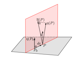
Let $\eta$ be a unit smooth vector field in $\mathbbm{E}^{3}$ and $\Delta_{\eta}$ be a plane field distribution orthogonal to $\eta.$ The second fundamental form of $\Delta_{\eta}$ is the bilinear form

$$II(X,Y)=\frac{1}{2}\langle\nabla_{X}Y+\nabla_{Y}X,\eta\rangle$$

where $X$ and $Y$ are smooth vector fields generating $\Delta_{\eta}$, see [13] and [18].

The normal curvature of $\Delta_{\eta}$ is given by

$$k_{\eta}(X)=\frac{II(X,X)}{I(X,X)},\;\;\;I(X,Y)=\langle X,Y\rangle$$

Following the classical approach of principal curvature lines (see [1], [23], [24], [26]) the extremal values of $k_{\eta}$ restricted to the plane field $\Delta_{\eta}$ are called $\eta-$principal curvatures (denoted by $k_{1}\leq k_{2}$) and the associated directions are called $\eta-$principal directions (denoted by $e_{1}$ and $e_{2}$). The integral curves of $e_{1}$ and $e_{2}$ are called $\eta-$principal lines, defining the two $\eta-$principal foliations $\mathcal{F}_{i}(\eta)$, $i=1,2$. 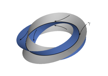The closed integral curves are called $\eta-$principal cycles.

The main results are:

Theorem 1.

Let $\gamma$ be a $\eta-$principal cycle of length $L$ of the $\eta$-principal foliation $\mathcal{F}_{1}(\eta)$. Given $\varepsilon>0$ small, there is a smooth vector field $\eta_{\varepsilon}$ in $\mathfrak{X}_{\mathfrak{R}}^{r}(\mathbbm{E}^{3})$, such that $\eta_{\varepsilon}$ is $\varepsilon-C^{r}$ close to $\eta$, with $\gamma$ being a hyperbolic $\eta_{\varepsilon}-$principal cycle of $\mathcal{F}_{1}(\eta_{\varepsilon})$.

Theorem 2.

Consider the set $\mathcal{G}$ of $\mathfrak{X}_{\mathfrak{R}}^{r}(\mathbbm{E}^{3})$ such that, for $\eta\in\mathcal{G}$, all $\eta-$principal cycles of $\mathcal{F}_{1}(\eta)$ and $\mathcal{F}_{2}(\eta)$ are hyperbolic. Then $\mathcal{G}$ is dense in $\mathfrak{X}_{\mathfrak{R}}^{r}(\mathbbm{E}^{3})$.

In section 2 the basic definitions will be introduced. The main concepts are the $\eta-$principal line fields, whose integral curves are called $\eta-$principal curvature lines. They are associated to the normal curvature of a plane distribution defined by an unit vector field $\eta$. See [1]. After that, it is obtained the differential equation of the $\eta-$principal line field directions.

When the plane distribution $\Delta_{\eta}$ is integrable these concepts coincide with the classical theory of principal lines on surfaces of $\mathbbm{E}^{3}$, a classical subject of differential geometry of surfaces which were introduced by G. Monge (1796), [15]. The qualitative theory and global aspects of principal lines were initiated by C. Gutierrez and J. Sotomayor (1982). See [6], [9] and [24].

In Section 3, the first return map associated to a $\eta-$principal cycle is considered and its first derivative is obtained as a solution of a linear differential equation. It will be shown that generically $\eta-$principal cycles are hyperbolic. In order to obtain the main result of Theorem 1 we will make use of ideas and results of geometric control theory as developed in [20] in the context of Hamiltonian systems and geodesics.

In Sections 4 and 5 will be presented the proofs of Theorems 1 and 2.

In Section 6 examples of hyperbolic $\eta$-principal cycles are analyzed.

In Section 7 some concluding remarks are discussed.

In A the main theorem involving geometric control theory, that will be used in Section 4 is stated for completeness and convenience to the reader.

In B the topology of $\mathfrak{X}_{\mathfrak{R}}^{r}(\mathbbm{E}^{3})$ will be reviewed.

2 $\eta-$Principal lines associated to a plane field $\Delta_{\eta}$

In this section, we present some notions concerning the extrinsic geometry of vector fields and plane fields and results that will be used in this work. This section is inspired in the Aminov’s book [1, Chapter 1].

2.1 Normal curvature of a plane field

Let $\mathfrak{X}_{\mathfrak{R}}^{r}(\mathbbm{E}^{3})$ be the set of unit regular vector fields of class $C^{r}$ in $\mathbbm{E}^{3}$ with the $C^{r}-$topology of Whitney, see [11] and [17].

Associated to a vector field $\eta=(\eta_{1},\eta_{2},\eta_{3})\in\mathfrak{X}_{\mathfrak{R}}^{r}(\mathbbm{E}^{3})$ we have a plane distribution, or a plane field, which will be denoted by $\Delta_{\eta}$. For each $p$, $\Delta(p)$ is the plane having $\eta(p)/|\eta(p)|$ as unit normal vector. The plane distribution $\Delta_{\eta}$ is completely integrable if, and only if, $\langle\rm{curl}{(\eta)},\eta\rangle=0$, where $\langle\cdot,\cdot\rangle$ denotes the usual inner product in $\mathbbm{E}^{3}$, see Frobenius Theorem [25, page 192].

Consider a plane $\Delta_{0}$ of the distribution $\Delta_{\eta}$ passing through a point $P_{0}$ and a vector $dr=(ds,dv,dw)$, written in classical notation, contained in the plane such that $P_{0}P=P-P_{0}$ is in the direction of $dr$. At the point $P$, take the orthogonal projection $\overline{\eta}(P)$ over the plane defined by the normal vector $\eta(P_{0})$ and the direction $dr$ which determines an angle $\varphi$ with $\eta(P_{0})$, as shown in the Fig. 1. For an unit vector field $\eta$, we define the normal curvature in the direction $dr$, or normal curvature of the distribution $\Delta_{\eta}$, by

$$\displaystyle k_{\eta}(dr)=\lim_{P\rightarrow P_{0}}{\dfrac{-\varphi}{|dr|}}.$$ (1)

When ${P\rightarrow P_{0}}$ we have that $\sin{\varphi}$ and $\varphi$ are of the same infinitesimal order. Once $\overline{\eta}(P)$ and the projection of $\eta(P)$ on the plane defined by $\eta(P_{0})$ and the directional vector $dr$ we have that $\dfrac{\langle\overline{\eta}(P),dr\rangle}{|\overline{\eta}(P)|}=\dfrac{\langle\eta(P),dr\rangle}{|\eta(P)|}$ and $\sin{\varphi}=\dfrac{\langle\overline{\eta}(P),dr\rangle}{|\overline{\eta}(P)|\cdot|dr|}$, in a neighborhood of $P_{0}$ and so we can write

$$\eta(P)=\eta(P_{0})+D\eta\cdot dr+\mathcal{O}(dr),$$ (2)

where $D\eta$ denotes the differential of the vector field $\eta$ and $D\eta\cdot v$ denotes the derivative of $\eta$ in the direction of $v$. It follows that

$$k_{\eta}(dr) = \displaystyle\lim_{P\rightarrow P_{0}}{\frac{-\varphi}{|dr|}}=\lim_{P\rightarrow P_{0}}\frac{-\sin{\varphi}}{|dr|}=\lim_{P\rightarrow P_{0}}\frac{-\langle\overline{\eta}(P),dr\rangle}{|\overline{\eta}(P)|\cdot|dr|}\cdot\frac{1}{|dr|}$$

$$= \displaystyle\lim_{P\rightarrow P_{0}}\frac{-\langle\eta(P_{0})+D\eta\cdot dr+{\mathcal{O}}(dr),dr\rangle}{|\overline{\eta}(P)|\cdot|dr|^{2}}=-\frac{\langle D\eta\cdot dr,dr\rangle}{\langle dr,dr\rangle},$$

since $|\overline{\eta}(P)|\longrightarrow|\eta(P_{0})|=1$ as $P\rightarrow P_{0}$. For more details see Y. Aminov [1, page 8].

Figure 1: Geometric definition of normal curvature of the unit vector field $\eta$.

The normal curvature of the vector field $\eta$ or of the plane distribution $\Delta_{\eta}$

$$k_{\eta}(dr)=-\dfrac{\langle D\eta\cdot dr,dr\rangle}{\langle dr,dr\rangle},$$ (3)

depends only on the direction $dr$ and not on its norm. In the holonomic case, that is, when the plane distribution $\Delta_{\eta}$ is completely integrable, the normal curvature of the plane field in the direction $dr$ coincides with the notion of normal curvature associated to a surface. If we consider the direction $dr$ restricted to the unit circle $\mathbbm{S}^{1}$ there are two directions which corresponds to the maximum and to the minimum curvature of the plane field and these directions can be determined as follows.

Given an unit vector field $\eta=(\eta_{1},\eta_{2},\eta_{3})$, with $\eta_{i}=\eta_{i}(r)$, $r=(s,v,w)\in\mathbbm{E}^{3}$, $i=1,2,3$, class $C^{k}$ functions, $k\geqslant 2$, denote by $D\eta\cdot dr=$ $(d\eta_{1}(r),d\eta_{2}(r),d\eta_{3}(r))$, $dr=(ds,dv,dw)$ and $d\eta_{i}(dr)=\langle\nabla\eta_{i},dr\rangle$. Consider the multiplier Lagrange problem:

$$\nabla k_{\eta}(dr)=\lambda\cdot\nabla G(dr),\ \ G(dr)=\langle\eta,dr\rangle.$$ (4)

Differentiation of equation (3) with respect to the variable $dr$ leads to

$$Dk_{\eta}\cdot dr(v)= -\displaystyle\dfrac{\left(\langle D\eta\cdot v,dr\rangle+\langle D\eta\cdot dr,v\rangle\right)\cdot\langle dr,dr\rangle-2\langle dr,v\rangle\langle D\eta\cdot dr,dr\rangle}{{\langle dr,dr\rangle}^{2}}$$

$$= \displaystyle\dfrac{1}{{\langle dr,dr\rangle}^{2}}\left\langle 2\langle D\eta\cdot dr,dr\rangle\cdot dr-\langle dr,dr\rangle\cdot(D\eta+D\eta^{t})\cdot dr,v\right\rangle.$$

Thus,

$$\nabla k_{\eta}(dr)=\dfrac{1}{{\langle dr,dr\rangle}^{2}}\left(2\langle D\eta\cdot dr,dr\rangle\cdot dr-{\langle dr,dr\rangle}\cdot(D\eta+D\eta^{t})\cdot dr\right).$$

As $\nabla G(dr)=\eta$, we get the eigenvector equation

$$\dfrac{1}{\langle dr,dr\rangle^{2}}\left(2\langle D\eta\cdot dr,dr\rangle\cdot dr-\langle dr,dr\rangle\cdot(D\eta+D\eta^{t})\cdot dr\right)=\lambda\cdot\eta.$$ (5)

As $|\eta|=1$ and using the fact that $\langle\eta,dr\rangle=0$, computing the inner product between equation (5) and $\eta$ we get

$$\lambda=-\left\langle\dfrac{(D\eta+D\eta^{t})\cdot dr}{\langle dr,dr\rangle},\eta\right\rangle,$$ (6)

which together with equation (5) gives

$$2\langle D\eta\cdot dr,dr\rangle\cdot dr-\langle dr,dr\rangle\cdot(D\eta+D\eta^{t})\cdot dr+\langle dr,dr\rangle\langle(D\eta+D\eta^{t})\cdot dr,\eta\rangle\cdot\eta=0.$$ (7)

Evaluating the inner product of equation (7) with the vector $dr\wedge\eta$, where $\wedge$ denotes the usual wedge product in $\mathbbm{R}^{3}$, it is obtained another equivalent form to the equation of eigenvectors

$$((D\eta+D\eta^{t})\cdot dr,dr,\eta)=0.$$ (8)

Using that $(D\eta^{t}-D\eta)\cdot dr=dr\wedge{\rm{curl}}(\eta)$, where $\rm{curl}(\eta)$ denotes the curl(rotational) of the vector field $\eta$ and $D\eta^{t}$ the transpose of $D\eta$, equation (8) can be written as

$$(2D\eta\cdot dr+D\eta^{t}\cdot dr-D\eta\cdot dr,dr,\eta)= 0$$

$$2(D\eta\cdot dr,dr,\eta)+(dr\wedge{\rm{curl}}(\eta),dr,\eta)= 0$$

$$2(D\eta\cdot dr,dr,\eta)+\left\langle\langle dr,dr\rangle\cdot{\rm{curl}}(\eta)-\langle dr,{\rm{curl}}(\eta)\rangle\cdot dr,\eta\right\rangle= 0,$$

and so the system

$$2(D\eta\cdot dr,dr,\eta)+\left\langle{\rm{curl}}(\eta),\eta\right\rangle\cdot\langle dr,dr\rangle= 0$$ (9)

$$\langle dr,\eta\rangle= 0$$

or equivalently,

$$((D\eta+D\eta^{t})\cdot dr,dr,\eta)= 0$$ (10)

$$\langle dr,\eta\rangle= 0$$

characterizes the maximum and minimum directions of the operator $k_{\eta}$ restricted to the plane defined by equation $\langle dr,\eta\rangle=0$.

Note that the term $(D\eta\cdot dr,dr,\eta)$ which appears in the first equation of the system (9) is related to the geodesic torsion $\tau_{g}=\dfrac{(D\eta\cdot dr,dr,\eta)}{\langle dr,dr\rangle}$ of the vector field $\eta$ in the direction $dr$, see [1, page 49]. Therefore, the system (9) can be rewritten as

$$2\tau_{g}+\left\langle{\rm{curl}}(\eta),\eta\right\rangle= 0$$ (11)

$$\langle dr,\eta\rangle= 0.$$

In the next lemma we will show that the vector field $\eta$ does not need to be unit in order to study the system of equations (9).

Lemma 1.

The system of equations (9) does not change when $\eta$ is multiplied by a non null scalar function $f(r)=f(s,v,w)$.

Proof.

Multiplying the vector field $\eta$ by the scalar function $f(r)$ it follows that

$$(2D(f(r)\eta)\cdot dr,dr,f(r)\eta)+\left\langle{\rm{curl}}(f(r)\eta),f(r)\eta\right\rangle\cdot\langle dr,dr\rangle= 0$$

$$2((\nabla f(r)\cdot dr)\eta+f(r)D\eta\cdot dr,dr,f(r)\eta)+\langle\nabla f(r)\wedge\eta+f(r){\rm{curl}}(\eta),f(r)\eta\rangle\cdot\langle dr,dr\rangle= 0$$

$$2(f(r))^{2}(D\eta\cdot dr,dr,\eta)+(f(r))^{2}\left\langle{\rm{curl}}(\eta),\eta\right\rangle\cdot\langle dr,dr\rangle= 0$$

$$(f(r))^{2}\cdot\left[(2D\eta\cdot dr,dr,\eta)+\left\langle{\rm{curl}}(\eta),\eta\right\rangle\cdot\langle dr,dr\rangle\right]= 0.$$

As $\langle dr,\eta\rangle=0$ and $f(r)\neq 0$, the Lemma is proved. $\square$

Recall that $\dfrac{\langle D\eta\cdot dr,dr\rangle}{\langle dr,dr\rangle}=-k_{\eta}$ and let $\bigg{(}\dfrac{D\eta+D\eta^{t}}{2}\bigg{)}\cdot dr=S(dr)$. We can interpret the equation (5) as an eigenvector equation:

$$S(dr)-\langle S(dr),\eta\rangle\eta=-k_{\eta}\cdot dr.$$ (12)

The next proposition describes some properties of the operator which defines the left hand side of the eigenvector equation(12).

Proposition 1.

Let $P:\mathbbm{E}^{3}\longrightarrow\mathbbm{E}^{3}$ be defined by $P(v)=S(v)-\langle S(v),\eta\rangle\cdot\eta$, where $S:\mathbbm{E}^{3}\longrightarrow\mathbbm{E}^{3}$ is a linear symmetric operator and $\pi=\{v\in\mathbbm{E}^{3}:\langle v,\eta\rangle=0\}$. Then the following holds:

• The kernel of the operator $P$, which is denoted by ker$(P)$, is generically ker$(S)+S^{-1}(\eta)$ and in general is transversal to the plane $\pi$.

• The plane $\pi$ is invariant by $P$, that is, $P(\pi)\subseteq\pi$ and $P$ restricted to $\pi$ is a symmetric operator.

Proof.

The Item 1) follows directly from the definition of $P$. To conclude 2), we observe that for $u,v\in\pi$, $\langle P(u),\eta\rangle=\langle P(v),\eta\rangle=0$ and $\langle P(u),v\rangle=\langle S(u),v\rangle=\langle u,S(v)\rangle=\langle u,P(v)\rangle.$ $\square$

The Lagrange multiplier problem, restricted to the plane, defined by equation (4) has two critical solutions $k_{1}=k_{1}(p)$ and $k_{2}=k_{2}(p)$ whose opposite values are called $\eta-$principal values or $\eta-$principal curvatures.

We associate to them three directions which are called $\eta-$principal directions. The tangent curves to these directions are called $\eta-$principal curvature lines or simply $\eta-$principal lines.

The points at which the $\eta$-principal curvatures coincide are called $\eta-$umbilic points and its set will be denoted by $\mathcal{U}(\eta)$, the points where only two principal curvatures coincide are called $\eta-$partially umbilic points.

The set of partially umbilic points of the plane field $\Delta_{\eta}$ is defined by $\mathcal{P}(\eta)=\{p\in\mathbbm{E}^{3}|\,k_{1}(p)=k_{2}(p)\}$.

Associated to the $\eta-$principal curvatures $k_{1}(p)$ and $k_{2}(p)$, the $\eta-$principal lines define two orthogonal foliations in $\mathbbm{E}^{3}-\mathcal{P}(\eta)$, which are denoted respectively by $\mathcal{F}_{1}(\eta)$ and $\mathcal{F}_{2}(\eta).$ They are called $\eta-$principal foliations of the plane field $\Delta_{\eta}$. The $\eta-$principal configuration is the triple $\mathbbm{P}(\eta)=\{\mathcal{F}_{1}(\eta),\mathcal{F}_{2}(\eta),\mathcal{P}(\eta)\}.$

The foliation defined by the integral curves of the vector field $\eta$, denoted by $\mathcal{F}_{\eta}$, is orthogonal to both $\eta-$principal foliations.

The system of equations (9) and (10) also characterizes the $\eta-$principal lines associated to the vector field $\eta$ or to the distribution $\Delta_{\eta}$.

The eigenvector equation obtained in (10) together with the condition $\langle\eta,dr\rangle=0$, is equivalent to the system of implicit differential equations

$$L_{1}\cdot ds^{2}+L_{2}\cdot dsdv+L_{3}\cdot dsdw+L_{4}\cdot dv^{2}+L_{5}\cdot dvdw+L_{6}\cdot dw^{2} =0$$ (13a)

$$\eta_{1}\cdot ds+\eta_{2}\cdot dv+\eta_{3}\cdot dw =0,$$ (13b)

where, $L_{i}$, $i=1,2,3,4,5,6$ are

$$L_{1} =\eta_{1}\left(\dfrac{\partial\eta_{3}}{\partial v}-\dfrac{\partial\eta_{2}}{\partial w}\right)+\eta_{2}\left(\dfrac{\partial\eta_{3}}{\partial s}+\dfrac{\partial\eta_{1}}{\partial w}\right)-\eta_{3}\left(\dfrac{\partial\eta_{2}}{\partial s}+\dfrac{\partial\eta_{1}}{\partial v}\right),$$

$$L_{2} =-2\eta_{1}\dfrac{\partial\eta_{3}}{\partial s}+2\eta_{2}\dfrac{\partial\eta_{3}}{\partial v}-2\eta_{3}\left(\dfrac{\partial\eta_{2}}{\partial v}-\dfrac{\partial\eta_{1}}{\partial s}\right),$$

$$L_{3} =2\eta_{1}\dfrac{\partial\eta_{2}}{\partial s}+2\eta_{2}\left(\dfrac{\partial\eta_{3}}{\partial w}-\dfrac{\partial\eta_{1}}{\partial s}\right)-2\eta_{3}\dfrac{\partial\eta_{2}}{\partial w},$$ (14)

$$L_{4} =-\eta_{1}\left(\dfrac{\partial\eta_{3}}{\partial v}+\dfrac{\partial\eta_{2}}{\partial w}\right)-\eta_{2}\left(\dfrac{\partial\eta_{3}}{\partial s}-\dfrac{\partial\eta_{1}}{\partial w}\right)+\eta_{3}\left(\dfrac{\partial\eta_{2}}{\partial s}+\dfrac{\partial\eta_{1}}{\partial v}\right),$$

$$L_{5} =2\eta_{1}\left(\dfrac{\partial\eta_{2}}{\partial v}-\dfrac{\partial\eta_{3}}{\partial w}\right)-2\eta_{2}\dfrac{\partial\eta_{1}}{\partial v}+2\eta_{3}\dfrac{\partial\eta_{1}}{\partial w},$$

$$L_{6} =\eta_{1}\left(\dfrac{\partial\eta_{3}}{\partial v}+\dfrac{\partial\eta_{2}}{\partial w}\right)-\eta_{2}\left(\dfrac{\partial\eta_{3}}{\partial s}+\dfrac{\partial\eta_{1}}{\partial w}\right)+\eta_{3}\left(\dfrac{\partial\eta_{2}}{\partial s}-\dfrac{\partial\eta_{1}}{\partial v}\right),$$

Equivalently, assuming that $\eta_{1}\neq 0$, we can determine $ds$ in (13b), and thus obtain the system

$$L(s,v,w)dw^{2}+M(s,v,w)dwdv+N(s,v,w)dv^{2}=0,$$ (15a)

$$\eta_{1}(s,v,w)ds+\eta_{2}(s,v,w)dv+\eta_{3}(s,v,w)dw=0.$$ (15b)

where, $L,M,N$ are

$$L(s,v,w) =\eta_{1}(\eta_{1}^{2}+\eta_{3}^{2})\left(\dfrac{\partial\eta_{3}}{\partial v}+\dfrac{\partial\eta_{2}}{\partial w}\right)-\eta_{3}(\eta_{1}^{2}+\eta_{3}^{2})\left(\dfrac{\partial\eta_{1}}{\partial v}+\dfrac{\partial\eta_{2}}{\partial s}\right)$$

$$+\eta_{2}(\eta_{3}^{2}-\eta_{1}^{2})\left(\dfrac{\partial\eta_{1}}{\partial w}+\dfrac{\partial\eta_{3}}{\partial s}\right)+2\eta_{1}\eta_{2}\eta_{3}\left(\dfrac{\partial\eta_{1}}{\partial s}-\dfrac{\partial\eta_{3}}{\partial w}\right),$$

$$M(s,v,w) =-2\eta_{2}(\eta_{1}^{2}+\eta_{3}^{2})\left(\dfrac{\partial\eta_{1}}{\partial v}+\dfrac{\partial\eta_{2}}{\partial s}\right)+2\eta_{3}(\eta_{1}^{2}+\eta_{2}^{2})\left(\dfrac{\partial\eta_{3}}{\partial s}+\dfrac{\partial\eta_{1}}{\partial w}\right)$$

$$+2\eta_{1}(\eta_{2}^{2}-\eta_{3}^{2})\dfrac{\partial\eta_{1}}{\partial s}+2\eta_{1}(\eta_{1}^{2}+\eta_{3}^{2})\dfrac{\partial\eta_{2}}{\partial v}-2\eta_{1}(\eta_{1}^{2}+\eta_{2}^{2})\dfrac{\partial\eta_{3}}{\partial w},$$

$$N(s,v,w) =-\eta_{1}(\eta_{1}^{2}+\eta_{2}^{2})\left(\dfrac{\partial\eta_{2}}{\partial w}+\dfrac{\partial\eta_{3}}{\partial v}\right)+\eta_{3}(\eta_{1}^{2}-\eta_{2}^{2})\left(\dfrac{\partial\eta_{1}}{\partial v}+\dfrac{\partial\eta_{2}}{\partial s}\right)$$

$$+\eta_{2}(\eta_{1}^{2}+\eta_{2}^{2})\left(\dfrac{\partial\eta_{1}}{\partial w}+\dfrac{\partial\eta_{3}}{\partial s}\right)+2\eta_{1}\eta_{2}\eta_{3}\left(\dfrac{\partial\eta_{2}}{\partial v}-\dfrac{\partial\eta_{1}}{\partial s}\right).$$

The singular set defined by $L(s,v,w)=$ $M(s,v,w)=$ $N(s,v,w)=0$ is the set of partially umbilic points.

In [8] was studied the behavior of the $\eta-$principal configuration $\mathbbm{P}(\eta)$ near the partially umbilic set when this set is a regular curve and under generic conditions. This configuration resemble that of principal curvature lines of hypersurfaces of $\mathbbm{E}^{4}$ near Darbouxian partially umbilic points, see [14].

Remark 1.

When the plane distribution $\Delta_{\eta}$ is Frobenius integrable, characterized by the condition $\langle{\rm{curl}}(\eta),\eta\rangle=0$, we are in the case of principal curvature lines of surfaces in $\mathbbm{E}^{3}$.

3 First return map associated to a $\eta$-principal cycle

In this section we will analyze the first return map associated to a closed $\eta$-principal line $\gamma$, determined by the system (10). We will assume that the curve $\gamma\colon\mathbbm{R}\longrightarrow\mathbbm{E}^{3}$ is parametrized by the arc length $s$ and has length $L$.

We will describe in this section the Poincaré map, or first return map, associated to a $\eta$-principal cycle $\gamma$ of the foliation $\mathcal{F}_{1}(\eta)$. Let us suppose, to fix the notation, that $\gamma$ is an orbit of a vector field $X_{1}$ defined in a tubular neighborhood of $\gamma$ and belonging to the plane field $\Delta_{\eta}$, that is, $X_{1}\in\Delta_{\eta}$.

Consider a vector field $\eta\in\mathfrak{X}_{\mathfrak{R}}^{r}(\mathbbm{E}^{3})$, $r\geqslant 2$, and let $\gamma$ be a closed $\eta-$principal line of the $\eta-$principal foliation $\mathcal{F}_{1}(\eta)$ and $X_{1}$ be a vector field in the plane distribution $\Delta_{\eta}$, such that $X_{1}(s)=X_{1}(\gamma(s))=\gamma^{\prime}(s)$, and $X_{2}(s)$ be the normal unit vector along the curve $\gamma$, $L-$periodic, such that $\{X_{1}(s),X_{2}(s)\}$ is a positively oriented basis of the plane of the distribution $\Delta_{\eta}$ which passes through $\gamma(s)$. Define a positively oriented orthonormal frame along $\gamma(s)$ given by $\{X_{1}(s),X_{2}(s),N(s)\}$, where $N(s)=X_{1}(s)\wedge X_{2}(s)$ and $N(s)=N(\gamma(s))=\eta(s)$. The Darboux equations are given by

$$DX_{1}\cdot X_{1} =k_{1}X_{2}+k_{2}N,$$

$$DX_{2}\cdot X_{1} =-k_{1}X_{1}+k_{3}N,$$ (16)

$$DN\cdot X_{1} =-k_{2}X_{1}-k_{3}X_{2}.$$

In the sequence will assume that the frame $\{X_{1}(s),X_{2}(s),N(s)\}$ is $L$-periodic, where $L$ is the length of $\gamma.$ Taking a double covering, always there exists a frame $\{X_{1}(s),X_{2}(s),N(s)\}$ which is $2L$-periodic. In this case it is necessary to consider the second return Poincaré map. See remark 3.

Let $V_{\delta}(\gamma)$ be a tubular neighborhood of the integral curve $\gamma$ as above and a parametrization $\alpha$ in the chart $(s,v,w)$, $L-$periodic in the variable $s$, given by

$$\alpha(s,v,w)=\gamma(s)+v\cdot X_{2}(s)+w\cdot N(s),$$ (17)

whose Jacobian matrix $D\alpha(s,v,w)$ relative to the basis $\{ds,dv,dw\}$ and $\{X_{1},$ $X_{2},N\}$ is given by

$$D\alpha(s,v,w)=\left(\begin{array}[]{ccc}1-k_{1}(s)v-k_{2}(s)w&0&0\\ -k_{3}(s)w&1&0\\ k_{3}(s)v&0&1\\ \end{array}\right).$$

Let $\mathbf{X}_{1}$ and $\mathbf{X}_{2}$ be $C^{r}$ local vector fields generating the plane field distribution $\Delta_{\eta}$ in a neighborhood $V_{\delta}(\gamma)$ of $\gamma$.

As $p=\alpha(s,v,w)$ and $dp=D\alpha(s,v,w)\cdot(ds,dv,dw)$, it follows from Hadamard’s Lemma that $\mathbf{X}_{1}$ and $\mathbf{X}_{2}$ are given in the chart $(s,v,w)$ by:

$$\mathbf{X}_{1}(p) =X_{1}(s)$$

$$+\bigg{(}A_{1}(s)v+A_{2}(s)w+\dfrac{1}{2}A_{10}(s)v^{2}+A_{11}(s)vw+\dfrac{1}{2}A_{01}(s)w^{2}+{\mathcal{O}}(3)\bigg{)}X_{2}(s)$$

$$+\bigg{(}B_{1}(s)v+B_{2}(s)w+\dfrac{(1}{2}B_{10}(s)v^{2}+B_{11}(s)vw+\dfrac{1}{2}B_{01}(s)w^{2}+{\mathcal{O}}(3)\bigg{)}N(s),\$$ (18)

$$\mathbf{X}_{2}(p) =(C_{1}(s)v+C_{2}(s)w+\dfrac{1}{2}C_{10}(s)v^{2}+C_{11}(s)vw+\dfrac{1}{2}C_{01}(s)w^{2}+{\mathcal{O}}(3)\bigg{)}X_{1}(s)$$

$$+\bigg{(}1+E_{1}(s)v+E_{2}(s)w+\dfrac{1}{2}E_{10}(s)v^{2}+E_{11}(s)vw+\dfrac{1}{2}E_{01}(s)w^{2}+{\mathcal{O}}(3)\bigg{)}X_{2}(s)$$

$$+\bigg{(}F_{1}(s)v+F_{2}(s)w+\dfrac{1}{2}F_{10}(s)v^{2}+F_{11}(s)vw+\dfrac{1}{2}F_{01}(s)w^{2}+{\mathcal{O}}(3)\bigg{)}N(s).$$ (19)

The unit vector field $\mathbf{N}(p)=N(\alpha(s,v,w))$ in the neighborhood $V_{\delta}(\gamma)$ is therefore given by

$$\mathbf{N}(p)=\dfrac{\mathbf{X}_{1}(p)\wedge\mathbf{X}_{2}(p)}{|\mathbf{X}_{1}(p)\wedge\mathbf{X}_{2}(p)|}=\mathbf{N}_{1}(p)\cdot X_{1}(s)+\mathbf{N}_{2}(p)\cdot X_{2}(s)+\mathbf{N}_{3}(p)\cdot N(s),$$ (20)

with

$$\mathbf{N}_{1}(p)= -B_{1}(s)v-B_{2}(s)w+(A_{1}(s)F_{1}(s)-\frac{B_{10}(s)}{2})v^{2}$$

$$+ (A_{1}(s)F_{2}(s)+A_{2}(s)F_{1}(s)-B_{11}(s))vw+b_{01}(s)w^{2}+{\mathcal{O}}(3),$$ (21)

$$\mathbf{N}_{2}(p)= -F_{1}(s)v-F_{2}(s)w+f_{10}(s)v^{2}+f_{11}(s)vw+f_{01}(s)w^{2}+{\mathcal{O}}(3),$$ (22)

$$\mathbf{N}_{3}(p)= \ 1-\frac{F_{1}(s)^{2}+B_{1}(s)^{2}}{2}v^{2}-(F_{2}(s)F_{1}(s)+B_{2}(s)B_{1}(s))vw$$

$$- \frac{F_{2}(s)^{2}+B_{2}(s)^{2}}{2}w^{2}+{\mathcal{O}}(3),$$ (23)

and

$$b_{01}= \frac{1}{2}\big{(}2A_{2}(s)F_{2}(s)-B_{01}(s)\big{)}$$

$$f_{01}= \frac{1}{2}\big{(}2F_{2}(s)E_{2}(s)+2B_{2}(s)C_{2}(s)-F_{01}(s)\big{)}$$

$$f_{11}= F_{1}(s)E_{2}(s)+F_{2}(s)E_{1}(s)+B_{1}(s)C_{2}(s)+B_{2}(s)C_{1}(s)-F_{11}(s)$$

$$f_{10}= \frac{1}{2}\big{(}2F_{1}(s)E_{1}(s)+2B_{1}(s)C_{1}(s)-F_{10}(s)\big{)}.$$

Evaluating the derivatives of $\mathbf{N}$ with respect to $s$, $v$ and $w$, it follows that:

$$\dfrac{\partial}{\partial s}\mathbf{N}(p) =\bigg{(}-k_{2}(s)+\Big{(}F_{1}(s)k_{1}(s)-\dfrac{d}{ds}(B_{1}(s)\Big{)}v+\Big{(}F_{2}(s)k_{1}(s)-\dfrac{d}{ds}(B_{2}(s)\Big{)}w$$

$$+{\mathcal{O}}(2)\bigg{)}\cdot X_{1}(s)+\bigg{(}-k_{3}(s)-\Big{(}B_{1}(s)k_{1}(s)+\dfrac{d}{ds}F_{1}(s)\Big{)}v-\Big{(}k_{1}(s)B_{2}(s)$$

$$+\dfrac{d}{ds}(F_{2}(s)\Big{)}w+{\mathcal{O}}(2)\bigg{)}\cdot X_{2}(s)+\bigg{(}\Big{(}-F_{1}(s)k_{3}(s)-B_{1}(s)k_{2}(s))\Big{)}v$$

$$+\Big{(}-F_{2}(s)k_{3}(s)-B_{2}(s)k_{2}(s)\Big{)}w+{\mathcal{O}}(2)\bigg{)}\cdot N(s),$$

$$\dfrac{\partial}{\partial v}\mathbf{N}(p)= \bigg{(}-B_{1}(s)+\Big{(}2A_{1}(s)F_{1}(s)-B_{10}(s)\Big{)}v+\Big{(}A_{2}(s)F_{1}(s)+A_{1}(s)F_{2}(s)-B_{11}(s)\Big{)}w$$

$$+{\mathcal{O}}(2)\bigg{)}\cdot X_{1}(s)+\bigg{(}-F_{1}(s)+2f_{10}(s)v+f_{11}(s)w+{\mathcal{O}}(2)\bigg{)}\cdot X_{2}(s)$$

$$+\bigg{(}-\Big{(}F_{1}(s)^{2}+B_{1}(s)^{2}\Big{)}v-\Big{(}F_{2}(s)F_{1}(s)+B_{2}(s)B_{1}(s)\Big{)}w+{\mathcal{O}}(2)\bigg{)}\cdot N(s),$$

$$\dfrac{\partial}{\partial w}\mathbf{N}(p)= \bigg{(}-B_{2}(s)+\Big{(}A_{2}(s)F_{1}(s)+A_{1}(s)F_{2}(s)-B_{11}(s)\Big{)}v+2b_{01}(s)w+{\mathcal{O}}(2)\bigg{)}\cdot X_{1}(s)$$

$$+ \bigg{(}-F_{2}(s)+f_{11}(s)v+2f_{01}(s)w+{\mathcal{O}}(2)\Bigg{)}\cdot X_{2}(s)$$

$$+ \bigg{(}-\Big{(}F_{2}(s)F_{1}(s)+B_{2}(s)B_{1}(s)\Big{)}v-\Big{(}F_{2}(s)^{2}+B_{2}(s)^{2}\Big{)}w+{\mathcal{O}}(2)\bigg{)}\cdot N(s).$$

As $p=\alpha(s,v,w)$, we have that $dp=D\alpha(s,v,w)\cdot(ds,dv,dw)$. Evaluating the mixed product and the equation of the plane (10) which characterizes the $\eta-$principal lines, given by $\Big{(}(D\mathbf{N}+D\mathbf{N}^{t})\cdot dp,dp,\mathbf{N}(p)\Big{)}=0$ and $\langle\mathbf{N}(p),dp\rangle=0$, we obtain

$$L_{1}\cdot ds^{2}+L_{2}\cdot dsdv+L_{3}\cdot dsdw+L_{4}\cdot dv^{2}+L_{5}\cdot dvdw+L_{6}\cdot dw^{2} =0,$$ (24)

$$M_{1}\cdot ds+M_{2}\cdot dv+M_{3}\cdot dw =0.$$ (25)

where $L_{i}=L_{i}(s,v,w)$, $i=1,2,3,4,5,6$ and $M_{i}=M_{i}(s,v,w)$, $i=1,2,3$ are given by

$$M_{1}(s,v,w) =(k_{3}(s)-B_{1}(s))v-B_{2}(s)w$$

$$+\Big{(}B_{1}(s)k_{1}(s)+A_{1}(s)F_{1}(s)-\frac{B_{10}(s)}{2}\Big{)}v^{2}$$

$$+(B_{2}(s)k_{1}(s)+B_{1}(s)k_{2}(s)+F_{1}(s)k_{3}(s)+A_{1}(s)F_{2}(s)$$

$$+A_{2}(s)F_{1}(s)-B_{11}(s))vw$$

$$+(k_{2}(s)B_{2}(s)+F_{2}(s)k_{3}(s)+b_{01}(s))w^{2}+{\mathcal{O}}(3),$$

$$M_{2}(s,v,w) =-F_{1}(s)v-F_{2}(s)w+f_{10}(s)v^{2}+f_{11}(s)vw+f_{01}(s)w^{2}+{\mathcal{O}}(3),$$

$$M_{3}(s,v,w) =1-\frac{F_{1}(s)^{2}+B_{1}(s)^{2}}{2}v^{2}-(F_{2}(s)F_{1}(s)+B_{2}(s)B_{1}(s))vw$$

$$-\frac{F_{2}(s)^{2}+B_{2}(s)^{2}}{2}w^{2}+{\mathcal{O}}(3).$$

$$L_{1}(s,v,w) =B_{1}(s)+k_{3}(s)-\Big{(}\big{(}B_{1}(s)+2k_{3}(s)\big{)}k_{1}(s)-F_{2}(s)k_{3}(s)-\big{(}2A_{1}(s)-B_{2}(s)\big{)}F_{1}(s)$$

$$+B_{10}(s)+\dfrac{d}{ds}F_{1}(s)\Big{)}v-\Big{(}\big{(}A_{2}(s)-2k_{3}(s)\big{)}F_{1}(s)+(A_{1}(s)-B_{2}(s))F_{2}(s)$$

$$+2B_{1}(s)k_{2}(s)-B_{2}(s)k_{1}(s)-B_{11}(s)-\dfrac{d}{ds}F_{2}(s)\Big{)}w+{\mathcal{O}}(2),$$

$$L_{2}(s,v,w) =+2\big{(}F_{1}(s)-k_{2}(s)\big{)}+\Big{(}2k_{1}(s)k_{2}(s)-\big{(}B_{1}(s)+k_{3}(s)\big{)}B_{2}(s)+F_{1}(s)F_{2}(s)$$

$$-4f_{10}(s)-2\dfrac{d}{ds}B_{1}(s)\Big{)}v+\Big{(}2B_{1}(s)k_{3}(s)+2k_{2}(s)^{2}-2k_{3}(s)^{2}-2F_{1}(s)k_{2}(s)$$

$$+2F_{2}(s)k_{1}(s)+F_{2}(s)^{2}-B_{2}(s)^{2}+2f_{11}(s)-2\dfrac{d}{ds}B_{2}(s)\Big{)}w+{\mathcal{O}}(2),$$

$$L_{3}(s,v,w) =F_{2}(s)+\Big{(}2B_{1}(s)^{2}+F1(s)^{2}+B_{1}(s)k_{3}(s)-2F_{1}(s)k_{2}(s)-F_{2}(s)k_{1}(s)$$

$$-f_{11}(s)\Big{)}v+\Big{(}F_{2}(s)F_{1}(s)+2B_{1}(s)B_{2}(s)-3F_{2}(s)k_{2}(s)+2B_{2}(s)k_{3}(s)$$

$$-2f_{01}(s)\Big{)}w+{\mathcal{O}}(2),$$

$$L_{4}(s,v,w) =-B_{1}(s)-k_{3}(s)+\Big{(}2A_{1}(s)F_{1}(s)-F_{2}(s)B_{1}(s)-B_{1}(s)k_{1}(s)-B_{10}(s)$$

$$-\dfrac{d}{ds}F_{1}(s)\Big{)}v+\Big{(}A_{1}(s)F_{2}(s)-F_{2}(s)B_{2}(s)-k_{1}(s)B_{2}(s)+A_{2}(s)F_{1}(s)$$

$$-B_{11}(s)-\dfrac{d}{ds}F_{2}(s)\Big{)}w+{\mathcal{O}}(2),$$

$$L_{5}(s,v,w) =-B_{2}(s)+\Big{(}A_{1}(s)F_{2}(s)+F_{1}(s)B_{1}(s)-B_{1}(s)k_{2}(s)-2F_{1}(s)k_{3}(s)$$

$$+A_{2}(s)F_{1}(s)-B_{11}(s)\Big{)}v+\Big{(}2F_{1}(s)B_{2}(s)-F_{2}(s)B_{1}(s)-2F_{2}(s)k_{3}(s)$$

$$-B_{2}(s)k_{2}(s)+2b_{01}(s)\Big{)}w+{\mathcal{O}}(2),$$

$$L_{6}(s,v,w) =\Big{(}F_{2}(s)B_{1}(s)-F_{1}(s)B_{2}(s)\Big{)}v+{\mathcal{O}}(2).$$

In the chart $(s,v,w)$ consider two transversal sections, $\Sigma_{1}=\{s=0\}$ and $\Sigma_{2}=\{s=L\}$. By construction, $\alpha(\Sigma_{1})=\alpha(\Sigma_{2})=\Sigma$ is a transversal section. Let $\gamma$ and a tubular neighborhood $V_{\delta}(\gamma)$, being $\gamma$ a $\eta-$principal cycle defined implicitly by the system of equations

$$\Big{(}(D\mathbf{N}(p)+D\mathbf{N}^{t}(p))\cdot dp,dp,\mathbf{N}(p)\Big{)} =0,$$ (26)

$$\langle\mathbf{N}(p),dp\rangle =0.$$ (27)

Define the Poincaré first return map in the chart $(s,v,w)$ by $\pi\colon\Sigma_{1}\longrightarrow\Sigma_{2}$, by $\pi(v_{0},w_{0})=\Big{(}v(L,v_{0},w_{0}),w(L,v_{0},w_{0})\Big{)}$, with $v(0,v_{0},w_{0})=v_{0}$ and $w(0,v_{0},w_{0})=w_{0}$. In order to calculate the derivative of the Poincaré map, we consider the system defined by equations (24) and (25) rewritten as

$$L_{1}+L_{2}\cdot\dfrac{dv}{ds}+L_{3}\cdot\dfrac{dw}{ds}+L_{4}\cdot\bigg{(}\dfrac{dv}{ds}\bigg{)}^{2}+L_{5}\cdot\dfrac{dv}{ds}\dfrac{dw}{ds}+L_{6}\cdot\bigg{(}\dfrac{dw}{ds}\bigg{)}^{2} =0,$$ (28)

$$M_{1}+M_{2}\cdot\dfrac{dv}{ds}+M_{3}\cdot\dfrac{dw}{ds} =0.$$ (29)

Differentiating implicitly the equations (28) and (29) in relation to the initial conditions $v_{0}$ and $w_{0}$ and evaluating at $(s,0,0)$, we have

$$\left(\begin{array}[]{cc}L_{2}&L_{3}\\ \cr M_{2}&M_{3}\end{array}\right)\cdot\dfrac{d}{ds}\left(\begin{array}[]{cc}\frac{\partial v}{\partial v_{0}}&\frac{\partial v}{\partial w_{0}}\\ \cr\frac{\partial w}{\partial v_{0}}&\frac{\partial w}{\partial w_{0}}\end{array}\right)=\left(\begin{array}[]{cc}-\dfrac{\partial L_{1}}{\partial v}&-\dfrac{\partial L_{1}}{\partial w}\\ \cr-\dfrac{\partial M_{1}}{\partial v}&-\dfrac{\partial M_{1}}{\partial w}\end{array}\right)\left(\begin{array}[]{cc}\frac{\partial v}{\partial v_{0}}&\frac{\partial v}{\partial w_{0}}\\ \cr\frac{\partial w}{\partial v_{0}}&\frac{\partial w}{\partial w_{0}}\end{array}\right).$$ (30)

For simplicity, we write the equation (30) as

$$A(s)\cdot\dfrac{d}{ds}U(s)=B(s)\cdot U(s).$$ (31)

Proposition 2.

Let $\gamma$ be a $\eta-$principal line parametrized by arc length $s$ of the foliation $\mathcal{F}_{1}(\eta).$ Suppose that there is a neighborhood $V_{\delta}(\gamma)$ of $\gamma$ such that the orthonormal frame $\{{X}_{1},{X}_{2},N\}$, $L-$periodic, is defined along $\gamma$ and the vector fields $\mathbf{X}_{1}(p)$ and $\mathbf{X}_{2}(p)$ given by (18) and (19) are defined in a neighborhood $V_{\delta}(\gamma)$. Then the following holds.

i) $B_{1}(s)=-k_{3}(s)$ and $F_{1}(s)-k_{2}(s)\neq 0$.

ii) The Poincaré return map $\pi\colon\Sigma_{1}\longrightarrow\Sigma_{2}$, where $\Sigma_{1}=\{s=0\}$ and $\Sigma_{2}=\{s=L\}$ are transversal sections to $\gamma$, in neighborhood $V_{\delta}(\gamma)$ is such that $D\pi(0)=U(L)$, where $U$ is the solution of the linear differential equation

$$\dot{U}=MU,$$ (32)

$$U(0)=I_{2},$$

with

$$M(s)=\left(\begin{array}[]{cc}M_{11}(s)&M_{12}(s)\\ &\\ -2k_{3}(s)&B_{2}(s)\end{array}\right),$$ (33)

and

$$M_{11}(s) =\dfrac{-\Big{(}F_{2}(s)+k_{1}(s)\Big{)}k_{3}(s)+\Big{(}B_{2}(s)-2A_{1}(s)\Big{)}F_{1}(s)+B_{10}(s)+\dfrac{d}{ds}F_{1}(s)}{2\Big{(}k_{2}(s)-F_{1}(s)\Big{)}},$$

$$M_{12}(s) =k_{3}(s)+\dfrac{k_{1}(s)B_{2}(s)-A_{2}(s)F_{1}(s)+\Big{(}2B_{2}(s)-A_{1}(s)\Big{)}F_{2}(s)+B_{11}(s)+\dfrac{d}{ds}F_{2}(s)}{2\Big{(}k_{2}(s)-F_{1}(s)\Big{)}}.$$

Proof.

As $\gamma$ is an integral curve of a vector field, implicitly defined by the system of equations

$$\Big{(}(D\mathbf{N}(p)+D\mathbf{N}^{t}(p))\cdot dp,dp,\mathbf{N}(p)\Big{)} =0,$$ (34)

$$\langle\mathbf{N}(p),dp\rangle =0,$$ (35)

we have that $dp=(ds,0,0)$ satisfies the equation (24), and therefore $L_{1}(s,0,0)$ $=L_{4}(s,0,0)=0$. As $\gamma$ is disjoint of the partially umbilic set we have $L_{2}(s,0,0)$ $\neq 0$. Therefore, it follows that $B_{1}(s)=-k_{3}(s)$ and $F_{1}(s)-k_{2}(s)\neq 0,$ which proofs ${\rm i)}$.

To prove item ${\rm ii)}$, consider the system of differential equations obtained in (30), with a simplified notation of (31). By item ${\rm i)}$ we have that $\det(A(s))=2\Big{(}F_{1}(s)-k_{2}(s)\Big{)}\neq 0$ and so the matrix $A(s)$ is invertible. With the initial conditions $v(0,v_{0},w_{0})=v_{0}$ and $w(0,v_{0},w_{0})=w_{0}$ we have $U(0)=I_{2}$ and therefore we can conclude that

$$\dfrac{d}{ds}U(s) =(A(s))^{-1}B(s)\cdot U(s)$$

$$U(0) =I_{2}.$$

This leads to the result since $(A(s))^{-1}B(s)=M(s)$. $\square$

Proposition 3.

In the case where the distribution $\Delta_{\eta}$ is completely integrable, we have:

i) $k_{3}(s)\equiv 0$.

ii) The derivative of the Poincaré map $D\pi(0)=U(L)$ is given by

$$U(L)=\left(\begin{array}[]{cc}\frac{\partial v}{\partial v_{0}}(L)&\frac{\partial v}{\partial w_{0}}(L)\\ \frac{\partial w}{\partial v_{0}}(L)&\frac{\partial w}{\partial w_{0}}(L)\end{array},\right)$$ (36)

where,

$$\frac{\partial w}{\partial v_{0}}(L) =0,$$

$$\frac{\partial w}{\partial w_{0}}(L) =\exp\bigg{(}\displaystyle\int_{0}^{L}B_{2}(s)ds\bigg{)},$$

$$\frac{\partial v}{\partial v_{0}}(L) =\exp\bigg{(}\displaystyle\int_{0}^{L}\frac{-\frac{d}{ds}F_{1}(s)}{F_{1}(s)-k_{2}(s)}ds\bigg{)},$$ (37)

$$\frac{\partial v}{\partial w_{0}}(L) =\frac{\partial v}{\partial v_{0}}(L)\int_{0}^{L}\frac{\partial v}{\partial v_{0}}(s)\frac{\partial w}{\partial w_{0}}(s)\frac{-B_{2}(s)\Big{(}2F_{2}(s)+k_{1}(s)\Big{)}-\frac{d}{ds}F_{2}(s)}{F_{1}(s)-k_{2}(s)}\ ds,$$

with   $\frac{\partial w}{\partial w_{0}}(s)=\exp\bigg{(}\displaystyle\int_{0}^{s}B_{2}(t)dt\bigg{)}$ and   $\frac{\partial v}{\partial v_{0}}(s)=\exp\bigg{(}\displaystyle\int_{0}^{s}\frac{-\frac{d}{dt}F_{1}(t)}{F_{1}(t)-k_{2}(t)}dt\bigg{)}$.

Proof.

From the equation $\omega=\langle\mathbf{N}(p),dp\rangle=0$ which defines the plane distribution $\Delta_{\eta}$ in a tubular neighborhood of the $\eta-$principal cycle $\gamma$ and evaluating $\omega$ in the system of coordinates $(s,v,w)$, we have

$$\omega(s,v,w)=M_{1}(s,v,w)\cdot ds+M_{2}(s,v,w)\cdot dv+M_{3}(s,v,w)\cdot dw$$ (38)

with $M_{1}(s,v,w)$, $M_{2}(s,v,w)$ and $M_{3}(s,v,w)$ as in equation (25).

Differentiating the differential form $\omega$ given by equation (38), we have

$$d\omega=-\dfrac{\partial M_{1}}{\partial v}ds\wedge dv-\dfrac{\partial M_{2}}{\partial w}ds\wedge dw+\Big{(}\dfrac{\partial M_{3}}{\partial v}-\dfrac{\partial M_{2}}{\partial w}\Big{)}dv\wedge dw.$$ (39)

Performing the calculations we have

$$\omega\wedge d\omega=f(s,v,w)\cdot ds\wedge dv\wedge dw=0,$$

where,

$$f(s,v,w)=M_{1}\cdot\bigg{(}\dfrac{\partial M_{3}}{\partial v}-\dfrac{\partial M_{2}}{\partial w}\bigg{)}+M_{2}\cdot\bigg{(}\dfrac{\partial M_{1}}{\partial w}-\dfrac{\partial M_{3}}{\partial s}\bigg{)}+M_{3}\cdot\bigg{(}\dfrac{\partial M_{2}}{\partial s}-\dfrac{\partial M_{1}}{\partial v}\bigg{)}.$$ (40)

Making use of the condition of integrability ($\omega\wedge d\omega=0$) we have $f(s,v,w)\equiv 0$. Thus, as $f(s,0,0)=-2k_{3}(s)=0$, the item i) is proved. Differentiating $f$ in relation to the variables $v$ and $w$ and evaluating at $(v,w)=(0,0)$, with $k_{3}(s)=0$, we have

$$f_{v}(s,0,0) =F_{1}(s)\Big{(}B_{2}(s)-2A_{1}(s)\Big{)}+B_{10}(s)-\dfrac{d}{ds}F_{1}(s),$$

$$f_{w}(s,0,0) =-F_{2}(s)A_{1}(s)-F_{1}(s)A_{2}(s)-B_{2}(s)k_{1}(s)+B_{11}(s)-\dfrac{d}{ds}F_{2}(s).$$

Solving equations $f_{v}(s,0,0)=0$ and $f_{w}(s,0,0)=0$, respectively in $B_{10}(s)$ and $B_{11}(s)$ and replacing in the system (32), with the condition $k_{3}(s)=0$, it is obtained

$$\dfrac{d}{ds}\left(\begin{array}[]{cc}\frac{\partial v}{\partial v_{0}}&\frac{\partial v}{\partial w_{0}}\\ \frac{\partial w}{\partial v_{0}}&\frac{\partial w}{\partial w_{0}}\end{array}\right)=\left(\begin{array}[]{cc}-\frac{\frac{d}{ds}F_{1}(s)}{F_{1}(s)-k_{2}(s)}&\frac{-B_{2}(s)\Big{(}F_{2}(s)+k_{1}(s)\Big{)}-\frac{d}{ds}F_{2}(s)}{F_{1}(s)-k_{2}(s)}\\ 0&B_{2}(s)\end{array}\right)\left(\begin{array}[]{cc}\frac{\partial v}{\partial v_{0}}&\frac{\partial v}{\partial w_{0}}\\ \frac{\partial w}{\partial v_{0}}&\frac{\partial w}{\partial w_{0}}\end{array}\right)$$

which can be solved using the initial conditions $\frac{\partial v}{\partial v_{0}}(0,0,0)=1$, $\frac{\partial v}{\partial w_{0}}(0,0,0)=0$, $\frac{\partial w}{\partial v_{0}}(0,0,0)=0$ and $\frac{\partial w}{\partial w_{0}}(0,0,0)=1$, getting the result. $\square$

Remark 2.

It is worth to note that equation (37) which determines $\dfrac{\partial v}{\partial v_{0}}(L)$ is exactly the derivative of the Poincaré map associated to a principal cycle $c:[0,L]\rightarrow\mathbbm{M}^{2}$ of principal curvature lines of surfaces obtained by Gutierrez and Sotomayor [24].

3.1 Hyperbolicity of a $\eta$-principal cycle

In this subsection we will present results on the hyperbolicity of $\eta$-principal cycles of a plane distribution in $\mathbb{E}^{3}$. We will say that a closed $\eta$-principal line $\gamma$ of length $L$ it is a hyperbolic $\eta$-principal cycle, if the derivative of the Poincaré map $D\pi(0)=U(L)$, obtained in the proposition 2, has no eigenvalues in the unit circle $\mathbbm{S}^{1}.$

Lemma 2.

With the same hypotheses as in Proposition (2), consider the perturbation $\eta_{\varepsilon}$ of the vector field $\eta$ in the neighborhood $V_{\delta}(\gamma)$ given by

$$\eta_{\varepsilon}(p)=\mathbf{N}_{\varepsilon}(p)=\frac{\mathbf{X}_{1\varepsilon}(p)\wedge\mathbf{X}_{2}(p)}{|\mathbf{X}_{1\varepsilon}(p)\wedge\mathbf{X}_{2}(p)|},$$ (41)

with

$$\mathbf{X}_{1\varepsilon}(p)= \mathbf{X}_{1}(p)+\varepsilon\Big{(}\phi_{1}(s)\cdot w+\phi_{2}(s)\cdot v^{2}+\phi_{3}(s)\cdot vw\Big{)}N(s),$$ (42)

and $\phi_{i}(s)$ of class $C^{\infty}$ for $i=1,2,3$. Then the conditions $B_{1}(s)=-k_{3}(s)$ and $F_{1}(s)-k_{2}(s)\neq 0$ are invariant by this perturbation and $\gamma$ is a closed $\eta$-principal line of length $L$ of $\mathcal{F}_{1}(\eta_{\varepsilon})$. The derivative of the Poincaré map $\pi_{\varepsilon}$ defined in $V_{\delta}(\gamma)\cap\Sigma$, where $\Sigma$ is a transversal section to $\gamma$, is given by $D\pi_{\varepsilon}(0)=V(L)$, and $V$ is a solution to Cauchy problem

$${}\dot{V}(s)= M_{\varepsilon}(s)V(s),$$

$$V(0)= I_{2},\ \ M_{\varepsilon}(s)=M_{\varepsilon}(s+L),$$ (43)

with

$$M_{\varepsilon}(s)=M(s)+\varepsilon\cdot\left(\begin{array}[]{cc}\dfrac{\phi_{1}(s)F_{1}(s)+2\phi_{2}(s)}{2\Big{(}k_{2}(s)-F_{1}(s)\Big{)}}&\dfrac{\Big{(}2F_{2}(s)+k_{1}(s)\Big{)}\phi_{1}(s)+\phi_{3}(s)}{2\Big{(}k_{2}(s)-F_{1}(s)\Big{)}}\\ &\\ 0&\phi_{1}(s)\end{array}\right),$$ (44)

and $M(s)$ is given by equation (33) of Proposition 2.

Proof.

Consider the vector fields $\mathbf{X}_{1\varepsilon}(p)$ (42) and $\mathbf{X}_{2}(p)$ (19) and the vector field

$$\mathbf{N}_{\varepsilon}(p)= \mathbf{N}(p)+\varepsilon\bigg{(}-\phi_{1}(s)w-\phi_{2}(s)v^{2}-\phi_{3}(s)vw+{\mathcal{O}}(3)\bigg{)}\cdot X_{1}(s)$$

$$+\varepsilon\bigg{(}\phi_{1}(s)C_{1}(s)vw+\phi_{1}(s)C_{2}(s)w^{2}+{\mathcal{O}}(3)\bigg{)}\cdot X_{2}(s)$$

$$\varepsilon\bigg{(}-\phi_{1}(s)B_{1}(s)vw-\Big{(}\phi_{1}(s)B_{2}(s)-\frac{\phi_{1}(s)^{2}\varepsilon}{2}\Big{)}w^{2}\bigg{)}\cdot N(s).$$

Calculating the derivatives of $\mathbf{N}_{\varepsilon}(p)$ in the directions $s$, $v$ and $w$, respectively, we have

$$\dfrac{\partial}{\partial s}\mathbf{N}_{\varepsilon}(p)= \dfrac{\partial}{\partial s}\mathbf{N}(p)+\varepsilon\cdot\Big{(}-\dfrac{d}{ds}\phi_{1}(s)w+{\mathcal{O}}(2)\Big{)}\cdot X_{1}(s)-\varepsilon\cdot\Big{(}\phi_{1}(s)k_{1}(s)w+{\mathcal{O}}(2)\Big{)}\cdot X_{2}(s)$$

$$- \varepsilon\cdot\Big{(}k_{2}(s)\phi_{1}(s)w+{\mathcal{O}}(2)\Big{)}\cdot N(s),$$

$$\dfrac{\partial}{\partial v}\mathbf{N}_{\varepsilon}(p)= \dfrac{\partial}{\partial v}\mathbf{N}(p)-\varepsilon\cdot\bigg{(}2\phi_{2}(s)v+\phi_{3}(s)w+{\mathcal{O}}(2)\bigg{)}\cdot X_{1}(s)$$

$$+ \varepsilon\cdot\Big{(}\phi_{1}(s)C_{1}(s)w+{\mathcal{O}}(2)\Big{)}\cdot X_{2}(s)-\varepsilon\cdot\Big{(}\phi_{1}(s)B_{1}(s)w+{\mathcal{O}}(2)\Big{)}\cdot N(s)$$

$$\dfrac{\partial}{\partial w}\mathbf{N}_{\varepsilon}(p) =\dfrac{\partial}{\partial w}\mathbf{N}(p)-\varepsilon\cdot\bigg{(}\phi_{1}(s)+\phi_{3}(s)v+{\mathcal{O}}(2)\bigg{)}\cdot X_{1}(s)$$

$$+\varepsilon\cdot\Big{(}\phi_{1}(s)C_{1}(s)v+2\phi_{1}(s)C_{2}(s)+{\mathcal{O}}(2)\Big{)}\cdot X_{2}(s)$$

$$-\varepsilon\bigg{(}\phi_{1}(s)B_{1}(s)v+\Big{(}2\phi_{1}(s)B_{2}(s)+\varepsilon\phi_{1}(s)^{2}\Big{)}w+{\mathcal{O}}(2)\bigg{)}\cdot N(s).$$

Calculating the mixed product and the equation of the plane that characterize the $\eta$-principal lines obtained in equation (10), given, respectively, by $\Big{(}(D\mathbf{N}_{\varepsilon}+D\mathbf{N}_{\varepsilon}^{t})\cdot dp,dp,\mathbf{N}_{\varepsilon}(p)\Big{)}=0$ and $\langle\mathbf{N}_{\varepsilon}(p),dp\rangle=0$, it follows that

$$L_{\varepsilon 1}\cdot ds^{2}+L_{\varepsilon 2}\cdot dsdv+L_{\varepsilon 3}\cdot dsdw+L_{\varepsilon 4}\cdot dv^{2}+L_{\varepsilon 5}\cdot dvdw+L_{\varepsilon 6}\cdot dw^{2} =0,$$

$$M_{\varepsilon 1}\cdot ds+M_{\varepsilon 2}\cdot dv+M_{\varepsilon 3}\cdot dw =0,$$ (45)

with $L_{\varepsilon i}=L_{\varepsilon i}(s,v,w)$, $i=1,2,3,4,5,6$ and $M_{\varepsilon i}=M_{\varepsilon i}(s,v,w)$, $i=1,2,3$, given by

$$M_{\varepsilon 1}(s,v,w) =(k_{3}(s)-B_{1}(s))v-\Big{(}B_{2}(s)+\varepsilon\phi_{1}(s)\Big{)}w+{\mathcal{O}}(2),$$

$$M_{\varepsilon 2}(s,v,w) =-F_{1}(s)v-F_{2}(s)w+{\mathcal{O}}(2),$$

$$M_{\varepsilon 3}(s,v,w) =1+{\mathcal{O}}(2),$$

$$L_{\varepsilon 1}(s,v,w) =L_{1}(s,v,w)+\varepsilon\cdot\bigg{(}\Big{(}\phi_{1}(s)F_{1}(s)+2\phi_{2}(s)\Big{)}v+\Big{(}\phi_{1}(s)\big{(}k_{1}(s)+F_{2}(s)\big{)}+\phi_{3}(s)\Big{)}w+{\mathcal{O}}(2)\bigg{)},$$

$$L_{\varepsilon 2}(s,v,w) =L_{2}(s,v,w)+\varepsilon\cdot\bigg{(}-\phi_{1}(s)\Big{(}B_{1}(s)+k_{3}(s)\Big{)}v-\Big{(}2\phi_{1}^{2}(s)\varepsilon+2\phi_{1}(s)B_{2}(s)$$

$$+2\phi_{1}(s)C_{1}(s)+2\dfrac{d}{ds}\phi_{1}(s)\Big{)}w+{\mathcal{O}}(2)\bigg{)},$$

$$L_{\varepsilon 3}(s,v,w) =L_{3}(s,v,w)-\varepsilon\cdot\bigg{(}\phi_{1}(s)C_{1}(s)v+2\phi_{1}(s)\Big{(}C_{2}(s)-k_{3}(s)-B_{1}(s)\Big{)}w+{\mathcal{O}}(2)\bigg{)},$$

$$L_{\varepsilon 4}(s,v,w) =L_{4}(s,v,w)+\varepsilon\cdot\bigg{(}-2\phi_{2}(s)v-\Big{(}\phi_{1}(s)F_{2}(s)+\phi_{1}(s)k_{1}(s)+\phi_{3}(s)\Big{)}w+{\mathcal{O}}(2)\bigg{)},$$

$$L_{\varepsilon 5}(s,v,w) =L_{5}(s,v,w)-\varepsilon\cdot\bigg{(}\phi_{1}(s)+\phi_{3}(s)v+\phi_{1}(s)\Big{(}k_{2}(s)-2F_{1}(s)\Big{)}w+{\mathcal{O}}(2)\bigg{)},$$

$$L_{\varepsilon 6}(s,v,w) =L_{6}(s,v,w)-\varepsilon\cdot\Big{(}F_{1}(s)\phi_{1}(s)v+{\mathcal{O}}(2)\Big{)}.$$

Substituting in the variational equation (30), we get

$$\left(\begin{array}[]{cc}L_{\varepsilon 2}&L_{\varepsilon 3}\\ \cr M_{\varepsilon 2}&M_{\varepsilon 3}\end{array}\right)\cdot\dfrac{d}{ds}\left(\begin{array}[]{cc}\frac{\partial v}{\partial v_{0}}&\frac{\partial v}{\partial w_{0}}\\ \cr\frac{\partial w}{\partial v_{0}}&\frac{\partial w}{\partial w_{0}}\end{array}\right)=\left(\begin{array}[]{cc}-\dfrac{\partial L_{\varepsilon 1}}{\partial v}&-\dfrac{\partial L_{\varepsilon 1}}{\partial w}\\ \cr-\dfrac{\partial M_{\varepsilon 1}}{\partial v}&-\dfrac{\partial M_{\varepsilon 1}}{\partial w}\end{array}\right)\left(\begin{array}[]{cc}\frac{\partial v}{\partial v_{0}}&\frac{\partial v}{\partial w_{0}}\\ \cr\frac{\partial w}{\partial v_{0}}&\frac{\partial w}{\partial w_{0}}\end{array}\right),$$ (46)

which we shall denote by

$$A_{\varepsilon}(s)\cdot\dfrac{d}{ds}U(s)=B_{\varepsilon}(s)\cdot U(s).$$ (47)

Evaluating in $(s,0,0)$, we have $L_{\varepsilon 1}(s)=L_{2}(s)$, $L_{\varepsilon 2}(s)=L_{2}(s)$, which ensure the invariance of the conditions $B_{1}(s)=-k_{3}$ and $F_{1}(s)-k_{2}(s)\neq 0$.

We also have in $(s,0,0)$ what $L_{\varepsilon 3}(s)=L_{3}(s)$, $M_{\varepsilon 2}(s)=M_{2}(s)$ and $M_{\varepsilon 3}(s)=M_{3}(s)$, and therefore the determinant $\det(A_{\varepsilon}(s))=2\Big{(}F_{1}(s)-k_{2}(s)\Big{)}\neq 0$. Therefore, the matrix $A_{\varepsilon}(s)$ is invertible. Let $v(0,v_{0},w_{0})=v_{0}$, $w(0,v_{0},w_{0})=w_{0}$ and $U(0)=I_{2}$. Therefore we conclude that

$$\dfrac{d}{ds}U(s) =(A_{\varepsilon}(s))^{-1}B_{\varepsilon}(s)\cdot U(s)$$

$$U(0) =I_{2}.$$

This leads to the result, since $(A_{\varepsilon}(s))^{-1}B_{\varepsilon}(s)=M_{\varepsilon}(s)$. $\square$

4 Proof of Theorem 1

Suppose that $\gamma$ is not a hyperbolic $\eta-$principal cycle of $\mathcal{F}_{1}(\eta)$ and consider a chart $(s,v,w)$, $L-$periodic in $s$, defined by equation (17). We will show that there is an vector field $\eta_{\varepsilon}$ sufficiently close to the vector field $\eta$, such that $\gamma$ is a hyperbolic $\eta_{\varepsilon}-$principal cycle of $\mathcal{F}_{1}(\eta_{\varepsilon})$, that is, suppose that an eigenvalue of $U(L)$ is in the unit circle $\mathbbm{S}^{1}$, being $U$ the solution of the Cauchy problem

$$\dot{U}(s)=M(s)\cdot U(s),$$ (48)

$$U(0)=I_{2},M(s)=M(s+L)$$

with $M(s)$ given by equation (33). The Cauchy problem (2) of Lemma 2 can be interpreted as a geometric control problem

$$\dot{V}(s)=M(s)V(s)+\sum_{i=1}^{3}u_{i}(s)E_{i}(s)V(s)=\left(M(s)+\sum_{i=1}^{3}u_{i}(s)E_{i}(s)\right)V(s),\ \ k\geqslant 1,$$ (49)

with controls

$$u_{1}(s) =\varepsilon\cdot\dfrac{\phi_{1}(s)F_{1}(s)+2\phi_{2}(s)}{2\Big{(}F_{1}(s)-k_{2}(s)\Big{)}},$$

$$u_{2}(s) =\varepsilon\cdot\dfrac{\phi_{1}(s)\Big{(}2F_{2}(s)+k_{1}(s)\Big{)}+\phi_{3}(s)}{2\Big{(}F_{1}(s)-k_{2}(s)\Big{)}},$$

$$u_{3}(s) =\varepsilon\cdot\phi_{1}(s),$$

with $\varepsilon$ $\in$ $\mathbbm{R}$, $\phi_{i}$ of compact support, and

$$E_{1}(s)=\left(\begin{array}[]{cc}1&0\\ 0&0\end{array}\right),\ \ \ E_{2}(s)=\left(\begin{array}[]{cc}0&1\\ 0&0\end{array}\right)\ \ \ E_{3}(s)=\left(\begin{array}[]{cc}0&0\\ 0&1\end{array}\right).$$

Let $\{B_{i}^{j}(s)\}$, $i=1,2,3$ and $j=1,2$ defined by

$$B_{i}^{1}(s)= E_{i}(s),$$

$$B_{i}^{2}(s)= [E_{i}(s),A(s)]=A(s)E_{i}(s)-E_{i}(s)A(s).$$

So it follows that,

$$B_{1}^{2}(s)=A(s)E_{1}(s)-E_{1}(s)A(s)=\left(\begin{array}[]{cc}0&*\\ -2k_{3}(s)&0\end{array}\right).$$

Taking $\overline{s}$ $\in$ $[0,L]$ such that $k_{3}(\overline{s})\neq 0$, we have that $\{E_{1}(\overline{s}),E_{2}(\overline{s}),E_{2}(\overline{s}),B_{1}^{2}(\overline{s})\}$ is a basis of the vector space $M_{2}(\mathbbm{R})$(matrices of order 2 with real coefficients). Therefore,

$${\rm Span}\{B_{i}^{j}(\overline{s})\ |\ i\in\{1,\ldots 3\},j=1,2\}=T_{I_{2}}M_{2}(\mathbbm{R}),$$ (50)

and so by the Theorem 3 in Appendix, the control system (49) is controllable in $[0,L]$. Therefore, we can get a vector field $\eta_{\varepsilon}$, $\varepsilon-C^{r}$ close to $\eta$, such that the eigenvalues of $D\pi_{\varepsilon}(0)=V(L)$, solution of the Cauchy problem (2) of Lemma 2, are not in the unit circle $\mathbbm{S}^{1}$. This ends the proof.

Remark 3.

The case where the orthonormal frame $\{X_{1}(s),X_{2}(s),N(s)\}$ is $2L$-periodic, we can consider the second return map to develop the analysis. This case happens when the derivative of the first return map is hyperbolic and has two negative real eigenvalues and so there are two non orientable invariant surfaces (Möbius strips) containing $\gamma$. See [12] or [16].

Figure 2: Invariant surfaces having topological type of Möbius strips.

Remark 4.

As it is well established in geometric theory of dynamical systems, a hyperbolic compact leaf $\gamma$ of an one dimensional foliation is stable under small deformations and the invariant manifolds (stable and unstable) asymptotic to $\gamma$ are smooth, see [5], [12] and [16]. For higher dimensional phenomena see [10] for example.

5 Proof of Theorem 2

Consider $\mathbbm{E}^{3}$ with the exhaustion of compacts $\{K_{m},m=1,\ldots,\infty\}$ defining the $C^{r}$ topology, $r\geq 3.$ See B.

Define the sets $\mathcal{G}(K_{m},L)$ of $\eta\in\mathfrak{X}_{\mathfrak{R}}^{r}(\mathbbm{E}^{3})$ such that all $\eta-$principal cycles of $\mathcal{F}_{i}(\eta)$ ($i=1,2$), with length smaller than $L$ and passing through the compact $K_{m}$ are hyperbolic.

Lemma 3.

The set $\mathcal{G}(K_{m},L)$ is residual in $\mathfrak{X}_{\mathfrak{R}}^{r}(\mathbbm{E}^{3})$.

Proof.

It is similar to the case of vector fields, see [16] and [17]. $\square$

Lemma 4.

The set

$$\mathcal{G}=\bigcap_{L=0}^{\infty}\bigcap_{m=1}^{\infty}\mathcal{G}(K_{m},L).$$

is dense in $\mathfrak{X}_{\mathfrak{R}}^{r}(\mathbbm{E}^{3})$.

Proof.

This is direct consequence of the fact that $\mathfrak{X}_{\mathfrak{R}}^{r}(\mathbbm{E}^{3})$ is a Baire space. See B or [17]. $\square$

6 Examples

In this section will be given examples of hyperbolic $\eta-$principal cycles of saddle and nodal type. Also a semi hyperbolic $\eta-$principal cycle is given.

Consider the vector fields $X_{1}=(-v+\lambda s(1-s^{2}-v^{2}),\ s+\lambda v(1-s^{2}-v^{2}),\ -aw)$, $X_{2}=(s+\varepsilon v,-\varepsilon s+v,0)\wedge X_{1}$ and let $\eta=(X_{1}\wedge X_{2})/|X_{1}\wedge X_{2}|$ a unitary vector field defined in an open set of $\mathbbm{R}^{3}$.

Proposition 4.

In the conditions above the unit circle $\gamma(t)=(\cos t,\sin t,0)$ is a $\eta$-principal cycle of the principal foliation $\mathcal{F}_{1}(\eta)$. Moreover, the eigenvalues of the Poincaré map are $\lambda_{1}=\exp(-4\pi\lambda)$ and $\lambda_{2}=\exp(\frac{2\pi a\varepsilon(\lambda-a)}{a\varepsilon+1})$ and this cycle is:

1. Hyperbolic of nodal type when $a\varepsilon>0$ and $\lambda(\lambda-a)<0$.

2. Hyperbolic of saddle type when $a\varepsilon>0$ and $\lambda(\lambda-a)>0$.

3. Semi hyperbolic of saddle node type when $a=0$ and $\lambda\neq 0$ or $a\neq 0$ and $\lambda=0$.

Proof.

Consider the change of coordinates given by:

$$s =(1-v_{1})\cos{t}$$

$$v =(1-v_{1})\sin{t}$$

$$w =w.$$

From equations (24) and (25), we obtain

$$L_{1}\cdot dt^{2}+L_{2}\cdot dtdv+L_{3}\cdot dtdw+L_{4}\cdot dv^{2}+L_{5}\cdot dvdw+L_{6}\cdot dw^{2} =0,$$ (51)

$$M_{1}\cdot dt+M_{2}\cdot dv+M_{3}\cdot dw =0,$$ (52)

with $L_{i}=L_{i}(t,v,w)$, $i=1,2,\ldots,6$ and $M_{i}=M_{i}(t,v,w)$, $i=1,2,3$. Here the new variable $v_{1}$ is written in the old notation. It can be verified, by straightforward calculations, that:

$$L_{3}(t,0,0)=2(a\varepsilon+1),\ \ L_{4}(t,0,0)=-2\lambda,\;\;\text{and}\;\;L_{i}(t,0,0)=0,\;\;i\neq 3,4.$$

$$M_{1}(t,0,0)=M_{3}(t,0,0)=0\;\;\text{and}\;\;M_{2}(t,0,0)=-1,$$

$$(L_{1})_{v}(t,0,0)=0,\;(L_{1})_{w}(t,0,0)=2a\varepsilon(a-\lambda),$$

$$(M_{1})_{v}(t,0,0)=-2\lambda,\;(M_{1})_{w}=(t,0,0)=0.$$

The calculations were corroborated with symbolic computations and we omitted these long expressions. We have that $\eta(\cos t,\sin t,0)=(\cos t,\sin t,0)$ and so the unit circle $\gamma$ is a $\eta-$principal cycle. The $\eta-$principal curvatures are $k_{1}=-1$ and $k_{2}=a\varepsilon.$

Differentiating equations (51) and (52) with respect to the initial conditions $v_{0}$ and $w_{0}$ and evaluating at $(t,0,0)$, we obtain the variational equation

$$\left(\begin{array}[]{cc}0&2(a\varepsilon+1)\\ \cr-1&0\end{array}\right)\cdot\dfrac{d}{dt}\left(\begin{array}[]{cc}\frac{\partial v}{\partial v_{0}}&\frac{\partial v}{\partial w_{0}}\\ \cr\frac{\partial w}{\partial v_{0}}&\frac{\partial w}{\partial w_{0}}\end{array}\right)=\left(\begin{array}[]{cc}0&2a\varepsilon(\lambda-a)\\ \cr 2\lambda&0\end{array}\right)\left(\begin{array}[]{cc}\frac{\partial v}{\partial v_{0}}&\frac{\partial v}{\partial w_{0}}\\ \cr\frac{\partial w}{\partial v_{0}}&\frac{\partial w}{\partial w_{0}}\end{array}\right).$$ (53)

or equivalently,

$$\dfrac{d}{dt}\left(\begin{array}[]{cc}\frac{\partial v}{\partial v_{0}}&\frac{\partial v}{\partial w_{0}}\\ \cr\frac{\partial w}{\partial v_{0}}&\frac{\partial w}{\partial w_{0}}\end{array}\right)=\left(\begin{array}[]{cc}-2\lambda&0\\ \cr 0&\frac{a\varepsilon(\lambda-a)}{a\varepsilon+1}\end{array}\right)\left(\begin{array}[]{cc}\frac{\partial v}{\partial v_{0}}&\frac{\partial v}{\partial w_{0}}\\ \cr\frac{\partial w}{\partial v_{0}}&\frac{\partial w}{\partial w_{0}}\end{array}\right).$$ (54)

Solving the linear differential equation (54) it follows that:

$$D\pi(0)=\left(\begin{array}[]{cc}\exp(-4\pi\lambda)&0\\ \cr 0&\exp\Big{(}\frac{2\pi a\varepsilon(\lambda-a)}{a\varepsilon+1}\Big{)}\end{array}\right),$$

which concludes the proof. $\square$

7 Concluding Remarks

The extrinsic geometry of vector fields and flows can be applied in the dynamic of mechanical systems, control systems, theoretical elasticity and fluid flows, see [1] and [4]. Also, in foliation theory the extrinsic geometry of leaves and flows is present, see [22] for a recent exposition on this subject.

In the case where $\Delta_{\eta}$ is integrable these foliations are exactly the principal curvature lines of an one parameter family of surfaces in $\mathbbm{E}^{3},$ a classical subject of differential geometry of surfaces which was introduced by G. Monge [15]. The qualitative theory and global aspects of principal lines were initiated by C. Gutierrez and J. Sotomayor [24] and is a current subject of research.

A correlated result, which corresponds to closed principal lines of three dimensional manifolds immersed in $\mathbbm{E}^{4}$ was obtained in [7].

The results of this work can be extended to regular plane fields defined in three dimensional Riemannian manifolds, following the natural concepts of curvature tensor and second fundamental forms of plane fields [18].

Appendix A Control Theory Concepts

We will now discuss some preliminary results of the control theory used in the previous section. For a broader reading in control theory we indicate Coron[Chapter 1] [3] and Rifford[Chapter 2] [19].

Consider a homogeneous linear differential equation control system $M_{n}(\mathbbm{R})$ (real matrices of order$n\geqslant 1$) of the form

$$\dot{X}(s)=A(s)X(s)+\sum_{i=1}^{k}u_{i}(s)B_{i}(s)X(s),\ \ k\geqslant 1,$$ (55)

with $X(s)$ in $M_{n}(\mathbbm{R})$; the controls $u_{i}(s)$ in $L^{1}([0,L]:\mathbbm{R}^{k})$, $k\geqslant 1$ and $s\in[0,L]$, $L>0$. The functions $A(s)$, $B_{i}(s)$ are continuous applications in $M_{n}(\mathbbm{R})$, with $i=1,2,\cdots,k$. Consider the Cauchy problem

$$\dot{X}(s)= A(s)X(s)+\sum_{i=1}^{k}u_{i}(s)B_{i}(s)X(s),\ \ k\geqslant 1,$$ (56)

$$X(0)= X_{0}.$$

Definition 1.

The control system (55) is completely controllable or controllable if, for each $(X_{0},X_{1})\in M_{n}(\mathbbm{R})\times M_{n}(\mathbbm{R})$, there exists a control $u(t)=(u_{1}(s),\ldots,u_{k}(s))$ in $L^{\infty}([0,L]\colon\mathbbm{R}^{k})$, such that the solution $X\in$ $C^{0}([0,L],M_{n}(\mathbbm{R}))$ of the Cauchy problem (56) satisfies $X(L)=X_{1}$.

The following theorem ensure us a sufficient condition for the controllability of (55), and is in Rifford and Ruggiero [20]. See also See also [3, Chapters 1,10] .

Theorem 3.

Let $L>0$, and smooth maps $s\in[0,L]\rightarrow$ $A(s)$, $B_{1}(s)\ldots$ $B_{k}(s)$ $\in$ $M_{n}(\mathbbm{R})$. Define $k$ sequences of maps

$$\{B_{1}^{j}\},\ldots\{B_{k}^{j}\}\colon[0,L]\rightarrow T_{I_{n}}M_{n}(\mathbbm{R}),$$

by

$${B_{i}^{0}(s)}:= {B_{i}(s)},$$

$$\vdots$$ (57)

$${B_{i}^{j}(s)}:= \frac{d}{ds}B_{i}^{j-1}(s)-[B_{i}^{j-1}(s),A(s)].$$

for all $s\in[0,L]$ and each $i\in\{1,\ldots k\}$. Suppose that there is a $\overline{s}\in[0,L]$ such that

$${\rm Span}\{B_{i}^{j}(\overline{s})\ |\ i\in\{1,\ldots k\},j\in\mathbbm{N}\}=T_{I_{n}}M_{n}(\mathbbm{R}).$$ (58)

Then, the control system (55) is controllable in $[0,L]$.

Appendix B Topology of unit vector fields in $\mathbbm{E}^{3}$

Here we will present, following Peixoto [17], a topology for the space of vector fields defined in non-compact manifolds.

Let $M^{n}=M$ a $n-$dimensional non-compact, the topology $C^{r}$ of Whitney $r\geqslant 1$, in space $\mathfrak{X}^{r}(M)$ of vectors fields in $M$ is defined as follows.

Let

$$K_{1}\subset K_{2}\subset K_{3}\subset\cdots\subset K_{i}\subset K_{i+1}\subset\cdots\subset M,$$ (59)

a decomposition of $M$ due to compact exhaustion $K_{i}$, with non-empty interior $\accentset{\circ}{K}_{i}\subset K_{i+1}$. If $X$is a vector field in $\mathfrak{X}^{r}(M)$ and $\delta(x)>0$ is a positive function in $M$, Let

$$\delta_{i}=\inf\left\{\delta(x),\ \ \ x\in K_{i}-\accentset{\circ}{K}_{i-1}\right\},\ \ \ K_{0}=\phi.$$

$$\mathcal{A}\Big{(}X,\delta(x)\Big{)}=\bigcap_{i=1}^{\infty}\{Y:d\Big{(}X,Y,K_{i}-\accentset{\circ}{K}_{i-1}\Big{)}<\delta_{i}\},$$ (60)

where $d$ is usual distance $C^{r}$ in compacts, see [11].

The set $\mathcal{A}\Big{(}X,\delta(x)\Big{)}$ forms a base of a neighborhood of $X$ in the topology in $\mathfrak{X}^{r}(M)$.

Remark 5.

An important observation is that this base does not depends on the decomposition of $M$, nor on the chosen of metric in each compact $K_{i}$.

Theorem 4.

The set $\mathfrak{X}^{r}(M)$, with the topology defined above, is a Baire space.

Proof.

See [11, Chapter 2] and [17].

Corollary 1.

The set $\mathfrak{X}_{\mathfrak{R}}^{r}(\mathbbm{E}^{3})$ of unit regular vector fields, with the induced topology of $\mathfrak{X}^{r}(\mathbbm{E}^{3})$, is a Baire space.

Proof.

See [11, Chapter 2]. $\square$

References

- Aminov [2000] Aminov, Y., 2000. The geometry of vector fields. Gordon and Breach Publishers, Amsterdam.
-
Boersma and Dray [1995]
Boersma, S., Dray, T., 1995. Parametric manifolds. I. Extrinsic approach.
J. Math. Phys. 36 (3), 1378–1393.
URL https://doi.org/10.1063/1.531127 - Coron [2007] Coron, J.-M., 2007. Control and nonlinearity. Vol. 136 of Mathematical Surveys and Monographs. American Mathematical Society, Providence, RI.
- Davydov [1994] Davydov, A. A., 1994. Qualitative theory of control systems. Vol. 141 of Translations of Mathematical Monographs. American Mathematical Society, Providence, RI, translated from the Russian manuscript by V. M. Volosov.
- Fenichel [1971/1972] Fenichel, N., 1971/1972. Persistence and smoothness of invariant manifolds for flows. Indiana Univ. Math. J. 21, 193–226.
- Garcia and Sotomayor [2009] Garcia, R., Sotomayor, J., 2009. Differential equations of classical geometry, a qualitative theory. Publicações Matemáticas. IMPA, Rio de Janeiro, 27o Colóquio Brasileiro de Matemática.
Garcia [1993]
Garcia, R. A., 1993. Hyperbolic principal cycles on hypersurfaces of . Ann. Global Anal. Geom. 11 (2), 185–196.
URL http://dx.doi.org/10.1007/BF00773456 - Gomes [2016] Gomes, A. J., 2016. Geometria extrínseca de campos de vetores em . http://repositorio.bc.ufg.br/tede/handle/tede/8636.
- Gutierrez and Sotomayor [1991] Gutierrez, C., Sotomayor, J., 1991. Lines of Curvature and Umbilic Points on Surfaces. Brasilian Math. Colloquium. IMPA.
- Hirsch [1973] Hirsch, M. W., 1973. Stability of compact leaves of foliations. Dynamical systems, (Proc. Sympos., Univ. Bahia, Salvador, 1971), 135–153.
- Hirsch [1976] Hirsch, M. W., 1976. Differential topology. Springer-Verlag, New York-Heidelberg, graduate Texts in Mathematics, No. 33.
- Hirsch et al. [1977] Hirsch, M. W., Pugh, C. C., Shub, M., 1977. Invariant manifolds. Lecture Notes in Mathematics, Vol. 583. Springer-Verlag, Berlin-New York.
Krouglov [2008]
Krouglov, V., 2008. The curvature of contact structures on 3-manifolds. Algebr.
Geom. Topol. 8 (3), 1567–1579.
URL https://doi.org/10.2140/agt.2008.8.1567 -
Lopes et al. [2015]
Lopes, D., Sotomayor, J., Garcia, R., 2015. Partially umbilic singularities of
hypersurfaces of . Bull. Sci. Math. 139 (4), 431–472.
URL https://doi.org/10.1016/j.bulsci.2014.10.005 - Monge [1796] Monge, G., 1796. Sur les lignes de courbure de la surface de l’ellipsoide. Journ. Ecole Polytech. II cah., 145–165.
- Palis and de Melo [1982] Palis, Jr., J., de Melo, W., 1982. Geometric theory of dynamical systems. Springer-Verlag, New York-Berlin, an introduction, Translated from the Portuguese by A. K. Manning.
Peixoto [1967]
Peixoto, M. M., 1967. On an approximation theorem of Kupka and Smale. J.
Differential Equations 3, 214–227.
URL https://doi.org/10.1016/0022-0396(67)90026-5 -
Reinhart [1977]
Reinhart, B. L., 1977. The second fundamental form of a plane field. J.
Differential Geom. 12 (4), 619–627.
URL http://projecteuclid.org/euclid.jdg/1214434230 -
Rifford [2014]
Rifford, L., 2014. Sub-Riemannian geometry and optimal transport.
SpringerBriefs in Mathematics. Springer, Cham.
URL http://dx.doi.org/10.1007/978-3-319-04804-8 - Rifford and Ruggiero [2012] Rifford, L., Ruggiero, R. O., 2012. Generic properties of closed orbits of Hamiltonian flows from Mañé’s viewpoint. Int. Math. Res. Not. IMRN (22), 5246–5265.
- Rogers [1911/1912] Rogers, G., 1911/1912. Some differential properties of the orthogonal trajectories of a congruence of curves. Proceedings of the Royal Irish Academy. Section A: Mathematical and Physical Sciences 29 (6), 92–117.
Rovenski and Walczak [2011]
Rovenski, V., Walczak, P., 2011. Topics in extrinsic geometry of
codimension-one foliations. SpringerBriefs in Mathematics. Springer, New
York, with a foreword by Izu Vaisman.
URL https://doi.org/10.1007/978-1-4419-9908-5 -
Sánchez-Bringas and Ramírez-Galarza [1995]
Sánchez-Bringas, F., Ramírez-Galarza, A. I., 1995. Lines of curvature
near umbilical points on surfaces immersed in . Ann. Global
Anal. Geom. 13 (2), 129–140.
URL https://doi.org/10.1007/BF01120328 - Sotomayor and Gutierrez [1982] Sotomayor, J., Gutierrez, C., 1982. Structurally stable configurations of lines of principal curvature. In: Bifurcation, ergodic theory and applications (Dijon, 1981). Vol. 98 of Astérisque. Soc. Math. France, Paris, pp. 195–215.
- Spivak [1999a] Spivak, M., 1999a. A comprehensive introduction to differential geometry V.1, 3rd Edition. Publish or Perish, INC.
- Spivak [1999b] Spivak, M., 1999b. A comprehensive introduction to differential geometry V.3, 3rd Edition. Publish or Perish, INC.
Voss [1880]
Voss, A., 1880. Geometrische Interpretation der Differentialgleichung
. Math. Ann. 16 (4), 556–559.
URL http://dx.doi.org/10.1007/BF01446224