Bottom quark mass effects in associated $WH$ production
with $H\to{b\bar{b}}$ decay through NNLO QCD

Abstract

We present a computation of NNLO QCD corrections to the production of a Higgs boson in association with a $W$ boson at the LHC followed by the decay of the Higgs boson to a ${b\bar{b}}$ pair. At variance with previous NNLO QCD studies of the same process, we treat $b$ quarks as massive. An important advantage of working with massive $b$ quarks is that it makes the use of flavor jet algorithms unnecessary and allows us to employ conventional jet algorithms to define $b$ jets. We compare NNLO QCD descriptions of the associated $WH({b\bar{b}})$ production with massive and massless $b$ quarks and also contrast them with the results provided by parton showers. We find ${\cal O}(5\%)$ differences in fiducial cross sections computed with massless and massive $b$ quarks. We also observe that much larger differences between massless and massive results, as well as between fixed-order and parton-shower results, can arise in selected kinematic distributions.

I Introduction

Detailed investigation of Higgs boson production in association with a $W$ boson is an important part of the LHC research program that aims at a comprehensive exploration of Higgs boson properties and electroweak symmetry breaking Chatrchyan:2013zna ; Aaboud:2017xsd ; Sirunyan:2017elk ; Aaboud:2018zhk ; Sirunyan:2018kst . Indeed, associated Higgs boson production gives us direct access to the $HWW$ coupling which is completely fixed in the Standard Model but can be modified in its extensions. Moreover, studies of the $pp\to WH$ process provide a unique way to study the Higgs coupling to $b$ quarks since, by selecting Higgs bosons with relatively high transverse momenta, one can identify $H\to{b\bar{b}}$ decays using substructure techniques Butterworth:2008iy ; Marzani:2019hun .

Interest in associated $WH$ production has inspired a large number of theoretical computations that provide refined descriptions of this process including QCD Han:1991ia ; Baer:1992vx ; Ohnemus:1992bd ; Mrenna:1997wp ; Spira:1997dg ; Djouadi:1999ht ; Brein:2003wg ; Brein:2011vx ; Brein:2012ne ; Ferrera:2011bk ; Ferrera:2013yga ; Campbell:2016jau ; Ferrera:2017zex ; Caola:2017xuq ; Gauld:2019yng and electroweak radiative corrections Ciccolini:2003jy ; Denner:2011id . The more recent theoretical efforts Ferrera:2011bk ; Ferrera:2013yga ; Campbell:2016jau ; Ferrera:2017zex ; Caola:2017xuq ; Gauld:2019yng focused on a comprehensive fully-differential description of associated production which consistently combines QCD corrections to the production and decay processes.

All fully-differential NNLO QCD computations mentioned above have the common feature that the decay of the Higgs boson to $b$ quarks is described under the assumption that $b$ quarks are massless. The same approximation is employed in the production subprocesses which involve gluon splitting into a ${b\bar{b}}$ pair or $b$ quarks that come directly from the proton. Although, given the high energy of the LHC, the massless approximation should be fairly adequate, there are a few reasons that make it interesting to explore $b$-quark mass effects in this process.

The first reason is that the phase space of the $pp\to WH$ process is large and that there are important kinematic distributions which can be sensitive to energy scales smaller than the total (partonic) energy of the process. In those cases the dependence on the $b$-quark mass can become more pronounced. A comparison of fixed-order computations, including higher-order ones, for $pp\to WH$ performed with massless and massive $b$ quarks will allow us to identify distributions and phase-space regions with enhanced sensitivity to the $b$-quark mass.

The second reason to employ massive $b$ quarks in a calculation is that in this case the splitting $g^{*}\to{b\bar{b}}$ becomes non-singular. This feature makes it possible to employ conventional jet algorithms to define $b$ jets. We remind the reader that in case of massless $b$ quarks, this is not possible and that a special partonic flavor jet algorithm Banfi:2006hf has to be used. The possibility to apply conventional jet algorithms is an important improvement since it makes theoretical computations and experimental analyses more aligned.

The third reason is the appearance of certain contributions in the $H\to{b\bar{b}}$ decay which cannot be properly described if $b$ quarks are treated as massless. It was pointed out in Ref. Caola:2017xuq that an interference of singlet $H\to g(g^{*}\to{b\bar{b}})$ and non-singlet $H\to(b^{*}\to bg)\bar{b}$ decay amplitudes forces us to keep the mass of the $b$ quark different from zero throughout the computation since otherwise unconventional soft quark divergences appear. Such studies have already been carried out in Ref. Primo:2018zby .

Motivated by these considerations, we extended the computation of NNLO QCD radiative corrections reported in Ref. Caola:2017xuq to include $b$-quark mass effects in the theoretical description of Higgs production in association with a vector boson. To this end, we combined the recent NNLO QCD description of the Higgs boson decay into two massive $b$ quarks Behring:2019oci with the computation of NNLO QCD corrections to the production process  Caola:2017xuq ; Caola:2019nzf which required small modifications because of the $b$-quark mass.

In addition to fixed-order computations, parton showers are widely used to provide theoretical predictions for collider experiments. In the context of associated Higgs production, they have been employed in Refs. Frixione:2005gz ; Hamilton:2009za ; Granata:2017iod ; Luisoni:2013kna ; Astill:2018ivh ; Bizon:2019tfo ; Alioli:2019qzz . For this reason, it is interesting to compare fixed-order and parton-shower results with each other. Although this has already been done in Ref. Caola:2017xuq , the need to use different jet algorithms in fixed-order massless and parton-shower computations did not allow a direct comparison of the two. The NNLO QCD computation with massive $b$ quarks described in this paper allows us to remedy this problem and compare fixed-order and parton-shower predictions using identical jet algorithms.

The remainder of the paper is organized as follows. In Section II we briefly review the NNLO QCD computation of radiative corrections to $pp\to WH$ Caola:2017xuq and $H\to{b\bar{b}}$ Behring:2019oci and discuss modifications needed in the computation of NNLO QCD corrections to the production process to accommodate massive $b$ quarks. In Section III we show numerical results for NNLO QCD corrections to $pp\to WH({b\bar{b}})$ with massive $b$ quarks and compare them to results of the massless computation. In Section IV we compare a parton-shower description of associated $WH$ production with fixed-order results. We conclude in Section V. A detailed discussion of modifications required to accommodate massive $b$ quarks in the NNLO QCD computation of Ref. Caola:2017xuq can be found in two appendices.

II Summary of NNLO QCD computations

In this section, we briefly review the computation of NNLO QCD radiative corrections to the associated production $pp\to WH$ and the $H\to{b\bar{b}}$ decay processes. An earlier computation of NNLO QCD corrections to $pp\to WH$ was described in Ref. Caola:2017xuq using the formulation of the nested soft-collinear subtraction scheme presented in Ref. Caola:2017dug . Since then, simple analytic formulas for the NNLO QCD corrections to the production of a color-singlet final state in hadron collisions were published in Ref. Caola:2019nzf . These formulas employ results for integrated double-unresolved soft and collinear subtraction terms computed in Refs. Caola:2018pxp and Delto:2019asp , respectively. To accommodate these developments, the code that allows us to compute NNLO QCD corrections to $pp\to WH$ was updated. In addition, we refined the description of the $H\to{b\bar{b}}$ decay with massless $b$ quarks using analytic results for NNLO QCD corrections to decays of color-singlet particles derived in Ref. Caola:2019pfz .

To accommodate massive $b$ quarks, we employed a recent computation Behring:2019oci of the NNLO QCD corrections to $H\to{b\bar{b}}$ that fully accounts for the $b$-quark mass. That computation is based on the nested soft-collinear subtraction scheme adapted to deal with massive particles. On the production side, a consistent description of $b$ quarks as massive particles forces us to work in a four-flavor scheme so that $b$ quarks are excluded from parton distributions. This feature leads to some changes to the renormalization procedure that we discuss in Appendix A. In addition, we have to modify the computation of NNLO QCD corrections to $pp\to WH$ to describe the splitting of a gluon into a massive ${b\bar{b}}$ pair, and the gluon vacuum polarization contributions due to massive $b$-quark loop.

We note that the gluon splitting contribution refers to the process $q_{i}q_{j}\to WH+(g^{*}\to{b\bar{b}})$ which is free of soft and collinear singularities thanks to the finite mass of the $b$ quark. The resulting logarithmically enhanced terms of the form $\log(s/m_{b}^{2})$ may, potentially, be large, but they do not appear to be particularly problematic from a numerical viewpoint. Hence, to describe these contributions, we calculate helicity amplitudes for the $q_{i}q_{j}\to WH{b\bar{b}}$ process, parametrize the $WH{b\bar{b}}$ phase space and perform numerical integration to compute observables of our choice.

Two-loop corrections to the $q_{i}\bar{q}_{j}W$ vertex caused by the gluon vacuum polarization due to a massive quark loop can be extracted from Refs. Kniehl:1989kz ; Rijken:1995gi ; Blumlein:2016xcy . We recomputed these contributions and found full agreement with the results presented in Ref. Kniehl:1989kz . For completeness, we provide the details of our calculation in Appendix B.

III The process $pp\to WH({b\bar{b}})$

In this section we present results for the associated production $pp\to WH({b\bar{b}})$ including $b$-quark mass effects. We begin by specifying how corrections to production and decay processes are combined. Since the Higgs boson is a scalar particle, these corrections can be put together in a straightforward manner. The only subtlety worth discussing is how to treat the total decay width of the Higgs boson that appears in the differential cross section for $pp\to WH({b\bar{b}})$ when it is computed in the narrow-width approximation. We begin by writing the cross section as follows Ferrera:2013yga

$${\rm d}\sigma_{WH({b\bar{b}})}={} {\rm d}\sigma_{WH}\times\frac{{\rm d}\Gamma_{{b\bar{b}}}}{\Gamma_{H}{}}={}{\rm Br}(H\to{b\bar{b}}){}\times{\rm d}\sigma_{WH}\times\frac{{\rm d}\Gamma_{{b\bar{b}}}}{\Gamma_{{b\bar{b}}}}\,.$$ (1)

We treat ${\rm Br}(H\to{b\bar{b}})$ as an input parameter and do not expand it in a series in $\alpha_{s}$. For numerical computations we take ${\rm Br}(H\to{b\bar{b}})=0.5824$, as recommended by the Higgs Cross Section Working Group deFlorian:2016spz .

Keeping the branching fraction fixed, we compute an expansion of Eq. (1) in $\alpha_{s}$ by first expanding the $WH$ cross section and the decay rate

$${\rm d}\sigma_{WH}={} \sum_{i=0}^{\infty}{\rm d}\sigma_{WH}^{(i)}\,, {\rm d}\Gamma_{{b\bar{b}}}={} \sum_{i=0}^{\infty}{\rm d}\Gamma_{{b\bar{b}}}^{(i)}\,,$$ (2)

then introducing normalized quantities to describe the decays

$${\rm d}\gamma^{(i)}={} \frac{\sum\limits_{k=0}^{i}{\rm d}\Gamma_{{b\bar{b}}}^{(k)}}{\sum\limits_{k=0}^{i}\Gamma_{{b\bar{b}}}^{(k)}}\,,$$ (3)

and, finally, defining physical cross sections computed through different orders in QCD perturbation theory

$$\begin{aligned} {\rm d}\sigma_{WH({b\bar{b}})}^{\rm LO}={}&{\rm Br}(H\to{b\bar{b}}){}\big{[}{\rm d}\sigma^{(0)}{\rm d}\gamma^{(0)}\big{]}\,,\\ {\rm d}\sigma_{WH({b\bar{b}})}^{\rm NLO}={}&{\rm Br}(H\to{b\bar{b}}){}\big{[}{\rm d}\sigma^{(0)}{\rm d}\gamma^{(1)}+{\rm d}\sigma^{(1)}{\rm d}\gamma^{(0)}\big{]}\,,\\ {\rm d}\sigma_{WH({b\bar{b}})}^{\rm NNLO}={}&{\rm Br}(H\to{b\bar{b}}){}\big{[}{\rm d}\sigma^{(0)}{\rm d}\gamma^{(2)}+{\rm d}\sigma^{(1)}{\rm d}\gamma^{(1)}+{\rm d}\sigma^{(2)}{\rm d}\gamma^{(0)}\big{]}\,.\end{aligned}$$ (4)

We note that ${\int}{\rm d}\gamma^{(i)}=1$ provided that the integration is performed over unrestricted phase space. An identical definition of the cross section was used in an earlier massless computation reported in Ref. Caola:2017xuq .

To present the results of our computation, we focus on the associated production process

$$pp\to W^{+}H\to(\nu_{e}\bar{e})({b\bar{b}}).$$ (5)

We treat both decay processes $W^{+}\to\nu_{e}\bar{e}$ and $H\to{b\bar{b}}$ in the narrow-width approximation. We set the Higgs boson mass to $M_{H}=125\leavevmode\nobreak\ \rm GeV$, the $W$-boson mass to $M_{W}=80.399\leavevmode\nobreak\ \rm GeV$ and the on-shell $b$-quark mass to $m_{b}=4.78\leavevmode\nobreak\ \rm GeV$. We note that the $b$-quark Yukawa coupling that enters the $H\to{b\bar{b}}$ decay is computed using the $\overline{\rm MS}$ $b$-quark mass calculated at $\mu=M_{H}$. However, since physical cross sections in Eq. (4) are proportional to the ratio ${\rm d}\Gamma_{{b\bar{b}}}/\Gamma_{{b\bar{b}}}$, the dependence on the Yukawa coupling cancels out (almost) completely in the results that are presented below. The top-quark mass is set to $m_{t}=173.2\leavevmode\nobreak\ \rm GeV$. We use the Fermi constant $G_{F}=1.16639\times 10^{-5}\leavevmode\nobreak\ \rm GeV^{-2}$ and the sine squared of the weak mixing angle $\sin^{2}\theta_{W}=0.2226459$. The width of the $W$ boson is taken to be $\Gamma_{W}=2.1054\leavevmode\nobreak\ \rm GeV$. Finally, we approximate the CKM matrix by an identity matrix.

We also need to specify the selection criteria that are used to define the $W(\nu_{e}\bar{e})\;H({b\bar{b}})$ final state. To this end, we require that an event contains at least two $b$ jets that are defined with the anti-$k_{t}$ jet algorithm Cacciari:2008gp ; Cacciari:2011ma . For the sake of comparison, we also calculate $WH({b\bar{b}})$ cross sections for massless $b$ quarks. In that case, we employ the flavor-$k_{t}$ jet algorithm Banfi:2006hf to describe massless $b$ jets. In both cases, we choose the jet radius $R=0.4$. Moreover, we impose the following cuts on pseudo-rapidities and transverse momenta of leptons and $b$ jets

$$\begin{aligned} &|\eta_{l}|<2.5\,,\quad p_{t,l}>15\leavevmode\nobreak\ \rm GeV\,,\\ &|\eta_{j,b}|<2.5\,,\quad p_{t,jb}>25\leavevmode\nobreak\ \rm GeV\,.\end{aligned}$$ (6)

Finally, following experimental analyses, we may employ an additional requirement that the vector boson has a transverse momentum of $p_{t,W}>150\leavevmode\nobreak\ \rm GeV$. We always state explicitly when this cut is used.

To present numerical results we use the five- and four-flavor parton distribution function sets NNPDF31_nnlo_as_0118 and NNPDF31_nnlo_as_0118_nf_4 for computations with massless and massive $b$ quarks, respectively. We employ NNLO PDFs to compute LO, NLO and NNLO cross sections in what follows. Moreover, both in massive and massless cases, we use $\alpha_{s}(M_{Z})=0.118$ and perform the running of the strong coupling at three loops with five active flavors.

For all cross sections the central value of the renormalization and factorization scales in the production process is set to one half of the invariant mass of the $WH$ system, i.e. $\mu_{r}=\mu_{f}=\tfrac{1}{2}\sqrt{(p_{W}+p_{H})^{2}}$, whereas the renormalization scale for the decay process is set to the Higgs boson mass, $\mu_{r,\rm{dec}}=M_{H}$. The uncertainty of the cross sections is obtained by varying the scale in the production process by a factor of two and, independently, by changing the decay scale by a factor of two as well. The total uncertainty is taken to be an envelope of these nine numbers.

Order	$b$ quarks	$\sigma_{\rm fid}\leavevmode\nobreak\ [\rm fb]$	$\sigma_{\rm fid}({\rm boosted})\leavevmode\nobreak\ [\rm fb]$
$\rm LO$	massive	$22.623^{+0.845}_{-1.047}$	$3.735^{+0.000}_{-0.016}$
	massless	$22.501^{+0.796}_{-1.007}$	$3.638^{+0.000}_{-0.009}$
$\rm NLO$	massive	$25.364(1)^{+0.778}_{-0.756}$	$4.586(1)^{+0.158}_{-0.141}$
	massless	$24.421(1)^{+0.852}_{-0.879}$	$4.333(1)^{+0.165}_{-0.154}$
$\rm NNLO$	massive	$24.225(4)^{+0.642}_{-0.742}$	$4.530(2)^{+0.071}_{-0.096}$
	massless	$22.781(3)^{+0.791}_{-0.898}$	$4.207(1)^{+0.097}_{-0.116}$

Table 1: Fiducial cross sections for $pp\to W^{+}H({b\bar{b}})$ at the $13\leavevmode\nobreak\ {\rm TeV}$ LHC at various orders of QCD perturbation theory calculated for massive and massless $b$ quarks. The label “boosted” implies that an additional cut is imposed on the $W$ boson’s transverse momentum, $p_{t,W}>150\leavevmode\nobreak\ \rm GeV$. The uncertainty is estimated using scale variation. The numerical integration error is reported in round brackets. See main text for details.

We begin by presenting fiducial cross sections for the process $pp\to W^{+}H({b\bar{b}})$ at the $13$ TeV LHC in Table 1. Comparing these results with massless predictions, we observe that the massive cross sections are systematically larger than the massless ones. The difference is very small at LO but increases when radiative corrections are included. At NLO, the differences range from about four percent, in case of the basic fiducial cuts, to six percent, if the additional $p_{t,W}>150\leavevmode\nobreak\ \rm GeV$ cut is applied. At NNLO, the differences between massive and massless results increase further and reach $6-7$ percent.

We note that these differences may be obscured by the scale variation uncertainties. This is indeed what happens at leading and, to some extent, also at next-to-leading order, whereas at NNLO the massive and massless cross sections differ from each other even if their scale variation uncertainties are accounted for.

We emphasize that the NNLO scale variation uncertainties shown in Table 1 are likely to be too conservative Gauld:2019yng . Indeed, it was shown in Ref. Gauld:2019yng that upon including a perturbative expansion of the $H\to b\bar{b}$ branching ratio in the definition of ${\rm d}\sigma_{WH}$, see Eq. (3), the NNLO scale uncertainty of the so-defined cross section reduces to a sub-percent level and becomes close to the uncertainty that is associated with the scale variation in the $WH$ production process without the decay. With this in mind, when discussing kinematic distributions, we only show results obtained with the central scale choice.

The ${\cal O}(5\%)$ differences between massive and massless fiducial cross sections can be traced back to gluon radiation in $H\to{b\bar{b}}$ decays. Indeed, it is well-known that the collinear radiation pattern of massive and massless $b$ quarks differs significantly. In case of massless $b$ quarks, we expect a logarithmic enhancement of the collinear gluon emission probability ${\rm d}{\cal P}\sim{\rm d}\theta^{2}/\theta^{2}$, where $\theta$ is the relative angle between the $b$ quark and the gluon momenta. This feature leads to a logarithmic dependence of the fiducial cross section on the clustering radius $R$. At the same time, when massive $b$ quarks radiate, the probability distribution becomes ${\rm d}{\cal P}\sim{\rm d}\theta^{2}/(\theta^{2}+m_{b}^{2}/E_{b}^{2})$, where $E_{b}$ is the energy of the radiating quark. This probability distribution implies that the collinear singularity is screened by the $b$-quark mass and that the cross-section dependence on the jet radius changes if $\Delta R<m_{b}/p_{t,b}$. We have checked that for the chosen value of the jet radius, the amount of radiation included in a $b$ jet is different for massless and massive quarks. This means that, in the case of radiative decay of the Higgs boson $H\to{b\bar{b}}g$, the acceptance of events with massless $b$ quarks is smaller, by about a factor of two, than the acceptance computed with massive $b$ quarks, when fiducial cuts described above are applied. We also observe that this difference is reduced if we consider larger jet radii or reduce the transverse momentum cut on $b$ jets.

Finally, it turns out that the ${\cal O}(y_{t}y_{b})$ interference of singlet $H\to g(g^{*}\to{b\bar{b}})$ and non-singlet $H\to(b^{*}\to bg)\bar{b}$ decay amplitudes, discussed in Ref. Caola:2017xuq , is a minor effect. For the fiducial cuts discussed above, it contributes to cross sections only at a sub-percent level and is, therefore, below the scale uncertainty and much smaller than the differences between massive and massless computations.

We will now proceed with the discussion of kinematic distributions. Since in an experimental analysis the Higgs boson can only be observed through its decay products, we will study kinematic distributions of the $b$- and $\bar{b}$-jet pair whose invariant mass is closest to the Higgs boson mass. Throughout this paper, we refer to such pairs of jets with the subscript $H({b\bar{b}})$, e.g. their four-momenta are written as $p_{H({b\bar{b}})}$ and their invariant masses as $M_{H({b\bar{b}})}$.

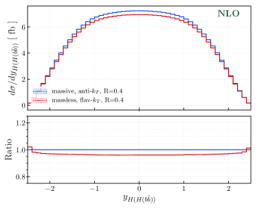
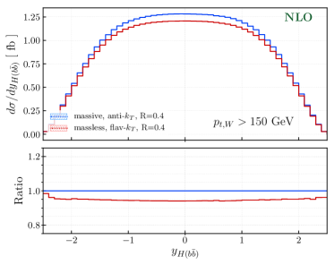
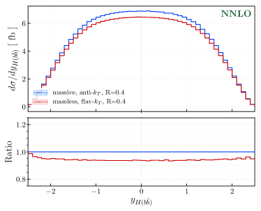
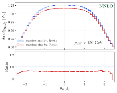
Figure 1: The rapidity distribution of the reconstructed Higgs boson calculated at NLO (upper plots) and NNLO (lower plots) for central values of the renormalization and factorization scales. Lower panes show ratios of massless to massive results. See text for details.

We begin by presenting the rapidity distribution of pairs of $b$ jets in Fig. 1. We observe that the distributions computed with massive and massless $b$ quarks are very similar and differ, to a good approximation, by an overall rescaling factor that can be inferred from the results for the cross sections reported in Table 1. Such behavior is expected given the well-known inclusiveness of rapidity distributions.

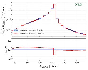
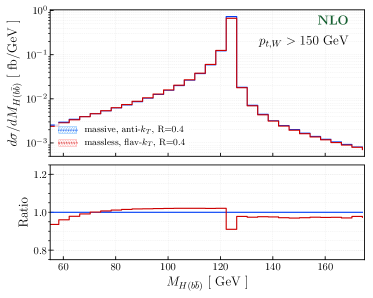
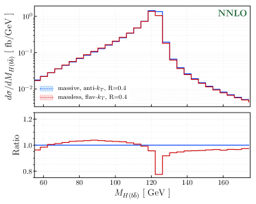
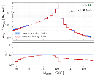
Figure 2: The invariant mass distribution of the two $b$ jets that best reconstruct the Higgs boson mass calculated at NLO (upper plots) and NNLO (lower plots) for central values of the renormalization and factorization scales. Lower panes show ratios of massless to massive results. See text for details.

We proceed with the invariant mass distribution of the two $b$ jets, $M_{H({b\bar{b}})}$, which is presented in Fig. 2. At leading order this distribution is described by a $\delta$-function, $\delta(M_{H({b\bar{b}})}^{2}-M_{H}^{2})$, but the situation becomes more complex when higher-order corrections are considered. In particular, if a $b$ quark from the decay is clustered with a gluon emitted in the production process, the invariant mass of two $b$ jets can exceed $M_{H}$ and, conversely, a three-body decay $H\to{b\bar{b}}g$ leads to two $b$ jets with an invariant mass that is smaller than $M_{H}$. Hence, already at NLO, the $M_{H({b\bar{b}})}$ distribution is non-vanishing both below and above $M_{H}$. We present the $M_{H({b\bar{b}})}$ distributions obtained at NLO and NNLO in Fig. 2. If the $p_{t,W}>150\leavevmode\nobreak\ \rm GeV$ cut is not applied, we observe that below the Higgs peak, the massless results are larger than the massive ones except at very low invariant masses. In the region above the peak, which is populated by events with radiative corrections to the production process, the two results are very similar to each other. In the most populated bin, adjacent to the Higgs boson mass, $M_{H({b\bar{b}})}=M_{H}$, the massive result is larger than the massless one; this feature drives the observed behavior for fiducial cross sections discussed earlier, c.f. Table 1. When the additional $p_{t,W}>150\leavevmode\nobreak\ \rm GeV$ cut is applied, the massless result stays below the massive one; we observe an $\mathcal{O}(15\%)$ difference at very low invariant masses which decreases when getting closer to the peak. Above the Higgs mass, we see a constant difference of about $10\%$.

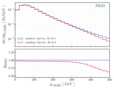
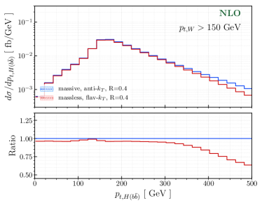
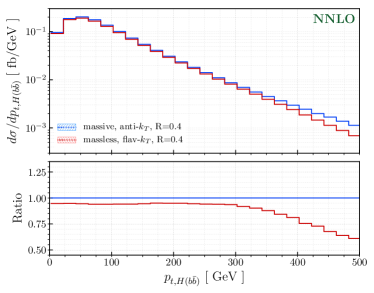
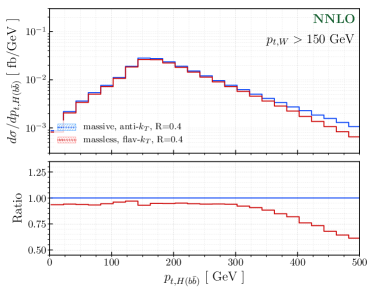
Figure 3: Reconstructed Higgs boson transverse momentum, see text for details, calculated at NLO (upper plots) and NNLO (lower plots) for central values of the renormalization and factorization scales. Lower panes show ratios of massless to massive results. See text for details.

Next, we consider the transverse momentum distribution of those $b$-jet pairs whose invariant mass is closest to the mass of the Higgs boson. The corresponding NLO and NNLO distributions are shown in Fig. 3. For standard fiducial cuts and for $p_{t,H(b\bar{b})}\lesssim 300\leavevmode\nobreak\ \rm GeV$, we observe that distributions computed with massive and massless $b$ quarks only differ by a re-scaling factor whose magnitude follows from the ratios of the fiducial cross sections. However, for higher transverse momenta, the difference between massive and massless calculations grows rapidly and becomes as large as $\mathcal{O}(25\%)$ at about $p_{t,H(b\bar{b})}\sim 400\leavevmode\nobreak\ \rm GeV$. This effect is driven by differences in clustering sequences of the employed jet algorithms and it is present already at leading order. Indeed, at very high transverse momenta, decay products of the Higgs boson are collimated and can be clustered within a single jet with zero bottom quantum number. Such events are then rejected by fiducial cuts since (at least) two $b$ jets are required. Since such a clustering starts to occur earlier in case of the flavor-$k_{t}$ jet algorithm, the massless result falls off more rapidly than the massive one. To some extent, this difference can be mitigated if a smaller clustering radius for the flavor-$k_{t}$ jet algorithm is chosen while the jet radius for the usual anti-$k_{t}$ algorithm is kept fixed. We have verified that such choices lead to increased values of $p_{t,H(b\bar{b})}$ at which massive and massless results start to depart from each other.

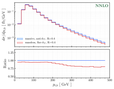
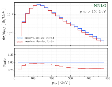
Figure 4: The transverse momentum distribution of the leading $b$ jet calculated at NNLO for central values of the renormalization and factorization scales. Lower panes show ratios of massless to massive results. See text for details.

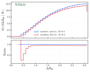
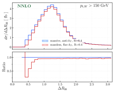
Figure 5: The distance $\Delta R_{H({b\bar{b}})}$ between the two $b$ jets used for Higgs boson reconstruction calculated at NNLO for central values of the renormalization and factorization scales. Lower panes show ratios of massless to massive results. See text for details.

Finally, we show the transverse-momentum distribution of the leading $b$ jet in Fig. 4 and the angular distance between the two $b$ jets $\Delta R_{H({b\bar{b}})}$ in Fig. 5. We observe significant differences between massive and massless results at large values of $p_{t,b}$ and at $\Delta R_{H({b\bar{b}})}\sim R$. Deviations at large transverse momenta in the $p_{t,b}$ distribution have the same origin as differences observed in $p_{t,H(b\bar{b})}$ distributions. As we discussed earlier, they are related to differences in the clustering of two $b$ jets into a single jet in the massive and massless cases.

In case of the $\Delta R_{H({b\bar{b}})}$ distributions, the massless to massive ratio is flat for large $\Delta R_{H({b\bar{b}})}\gtrsim 0.75$ jet separation but they become different for smaller values of $\Delta R_{H({b\bar{b}})}$. Again, these features are closely related to the behavior of the $p_{t,H(b\bar{b})}$ distributions since a small angular separation of the two $b$ jets corresponds to a boosted configuration from a Higgs boson with large transverse momentum.

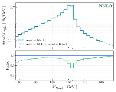
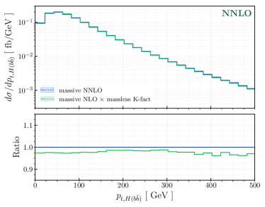
Figure 6: Comparison of approximate and exact NNLO distributions for central values of the renormalization and the factorization scales. Lower panes show ratios of the two distributions with respect to the exact calculation. See text for details.

As we already pointed out, some differences in kinematic distributions computed with massive and massless quarks arise already at leading order. If we assume that radiative effects are similar in massive and massless cases, one can construct approximate NNLO distributions from massive NLO computations and massless differential $K$-factors defined as ${\rm d}K={\rm d}\sigma_{\rm NNLO}/{\rm d}\sigma_{\rm NLO}$. We compare the (so constructed) approximate and exact NNLO distributions for $M_{H({b\bar{b}})}$ and $p_{t,H(b\bar{b})}$ in Fig. 6. We observe that such an approximation is only partially successful; it provides a decent description of the true $p_{t,H(b\bar{b})}$ distribution but does not capture all the details of the $M_{H({b\bar{b}})}$ spectrum.

IV Comparison with parton shower

Having discussed fixed-order calculations with massive and massless $b$ quarks, we turn to a comparison of these calculations with parton showers. Such a comparison is important because experimental analyses often rely on parton showers and one needs to understand their reliability by comparing them to fixed-order computations.

For our purposes, we use the POWHEG-BOX-V2 framework Nason:2004rx ; Frixione:2007vw ; Alioli:2010xd with the publicly available HWJ event generator Luisoni:2013kna constructed using the improved MiNLO method Hamilton:2012rf . It allows us to simulate the $pp\to W^{+}Hj$ process with NLO QCD accuracy. Moreover, upon integration over the resolved radiation, the NLO QCD result for $pp\to W^{+}H$ is obtained. For the parton shower we use Pythia8 Sjostrand:2007gs with the Monash tune Skands:2014pea . We simulate the $H\to{b\bar{b}}$ decay with Pythia8 that includes the matrix element correction that allows to describe $H\to{b\bar{b}}g$ decay in a reliable way. To stay as close as possible to fixed-order calculations, we use parton-shower results at the parton level, without hadronization and multi-parton interactions effects.

Using the POWHEG+Pythia8 setup and our fiducial cuts described in Sec. III, we obtain the following values for the cross sections

$$\sigma_{\rm fid}^{\texttt{PWHG+Pythia8}}={} 23.934(9)\leavevmode\nobreak\ \rm fb\,, \sigma_{\rm fid,boost}^{\texttt{PWHG+Pythia8}}={} 4.368(4)\leavevmode\nobreak\ \rm fb\,.$$ (7)

The second result shown in Eq. (7) is obtained by requiring that, in addition to standard fiducial cuts, the transverse momentum of the $W$ boson $p_{t,W}$ exceeds $150\leavevmode\nobreak\ {\rm GeV}$. The uncertainties shown in Eq. (7) correspond to numerical integration errors.

The parton-shower cross sections Eq. (7) differ from NNLO cross sections computed with massive $b$ quarks by about $2\%$ in the full fiducial region and by about $4\%$ if the additional $p_{t,W}$ cut is applied (c.f. Table 1). These differences are only natural given that the POWHEG+Pythia8+MiNLO setup is different compared to what we use to obtain fixed-order predictions, see Ref. Luisoni:2013kna for further details.

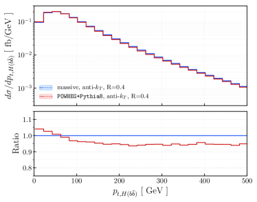
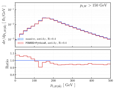
Figure 7: The transverse momentum distribution of two $b$ jets whose invariant mass is closest to the Higgs boson mass for central values of the renormalization and factorization scales. Lower panes show ratios of parton shower to massive fixed-order results. See text for details.

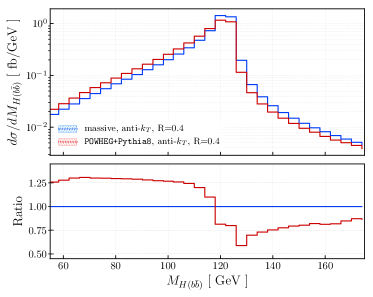
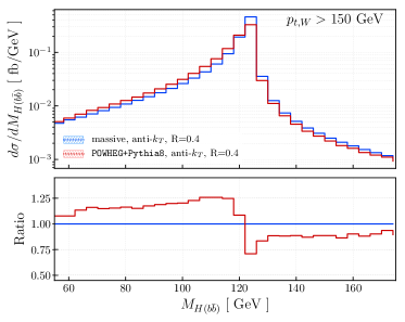
Figure 8: The invariant mass distribution of the two $b$ jets that best reconstruct the Higgs boson mass for central values of the renormalization and factorization scales. Lower panes show ratios of parton shower to massive fixed-order results. See text for details.

We proceed with the comparison of fixed-order and the parton-shower descriptions of selected kinematic distributions for a pair of $b$ jets whose invariant mass is closest to the mass of the Higgs boson. We present the transverse momentum distribution of such $b$-jet pairs in Fig. 7, and their invariant mass distribution in Fig. 8. In the case of the transverse momentum distribution, both with and without the additional $p_{t,W}$ cut, we see that in the region $p_{t,H(b\bar{b})}\gtrsim 100\leavevmode\nobreak\ \rm GeV$ the parton-shower result is smaller than the massive NNLO result by about five percent, whereas for transverse momenta below the peak of the distribution, $p_{t,H(b\bar{b})}\lesssim 50\leavevmode\nobreak\ \rm GeV$, the parton-shower prediction exceeds the fixed-order result by about five percent. We note that such behavior is expected since additional QCD radiation, simulated by a parton shower, reduces energies of the $b$ jets leading to a softer spectrum.

Differences between parton-shower predictions and the massive fixed-order NNLO result for the invariant mass of the ${b\bar{b}}$-system are more significant than in case of the transverse momentum distribution, c.f. Fig. 8. Below the Higgs peak we observe a $\mathcal{O}(25\%)$ excess of the parton-shower result over the fixed-order result; above the peak, parton-shower results are $\mathcal{O}(25\%)$ smaller than fixed-order results. We note that the parton-shower and the fixed-order distributions can be made well aligned provided that the fixed-order distribution is shifted along the $x$ axis by $\delta M_{{b\bar{b}}}\sim-4\leavevmode\nobreak\ {\rm GeV}$.

V Conclusions

In this paper, we discussed the associated production of the Higgs boson, $pp\to WH$, and the decay of the Higgs boson to ${b\bar{b}}$ pairs at the LHC. We included the NNLO QCD corrections to the production and decay processes, retaining the dependence on the $b$-quark mass. The inclusion of the $b$-quark mass in the calculation is important as it allows us to use realistic jet algorithms to describe $b$ jets, making theoretical and experimental analyses more aligned.

We compared theoretical predictions for the associated production that are obtained with massive and massless $b$ quarks. We observed ${\cal O}(6\%)$ differences between the two results once fiducial cuts are applied. Such relatively large differences can be traced back to different acceptances in radiative decays of the Higgs boson $H\to{b\bar{b}}g$ when they are computed in the massive and in the massless approximations for a standard set of fiducial volume cuts. We also found that radiative corrections to the production process are less sensitive to $b$-quark mass effects.

Interestingly, mass effects can become much more pronounced in kinematic distributions. For example, we observed large differences between massive and massless predictions in kinematic regions where $b$ jets have large transverse momenta. In these cases, differences in clustering algorithms employed with massive and massless partons, needed to unambiguously define a jet’s flavor, combine with rapidly changing distributions and lead to ${\cal O}(20\%)$ discrepancies between the theoretical predictions.

We note that in some cases such large discrepancies are driven by differences in lower-order distributions while massive and massless $K$-factors turn out to be similar. If this is the case, an approximate massive NNLO result may be constructed from massive NLO result and massless NNLO/NLO $K$-factor. We have identified the transverse momentum $p_{t,H(b\bar{b})}$ as one such observable. However, there are also other cases where the differences in NNLO distributions are driven by different (massive and massless) $K$-factors; if this is the case, the approximate distribution will not provide a decent description of the true result. This is the case, e.g., for the invariant mass $M_{H({b\bar{b}})}$.

Differences between massive NNLO QCD and parton-shower computations, discussed in Sec. IV, are easily understood if we assume that parent $b$ quarks lose more energy in a parton-shower computation than in a fixed-order one. This implies that shapes of, at least some, distributions in both cases are similar but the distributions themselves are shifted relative to each other, e.g. ${\rm d}\sigma^{(PS)}/{\rm d}x\;(x)\sim{\rm d}\sigma^{(FO)}/{\rm d}x\;(x+\delta_{x})$. We have found that, in case of the invariant mass of two hardest $b$ jets, $\delta_{x}\sim 4\leavevmode\nobreak\ {\rm GeV}$ which appears to be a rather natural value.

In summary, we studied effects of the $b$-quark mass on associated production of the Higgs boson, $pp\to WH$, followed by decay of the Higgs boson into a ${b\bar{b}}$ pair. Although such effects are not large, we found that they are typically larger than naively expected and that they can affect both fiducial cross sections and kinematic distributions in a somewhat unexpected way. We look forward to future studies of such effects in other processes relevant for the LHC phenomenology.

Acknowledgments: We would like to thank Gavin Salam for useful discussions as well as providing us with his private implementation of the flavor-$k_{t}$ algorithm Banfi:2006hf . This research is partially supported by BMBF grant 05H18VKCC1 and by the Deutsche Forschungsgemeinschaft (DFG, German Research Foundation) under grant 396021762 - TRR 257. The research of F.C. was partially supported by the ERC Starting Grant 804394 hipQCD.

Appendix A Renormalization

In this appendix, we discuss the details of the renormalization scheme that we adopt in this calculation. We work with $n_{f}=4$ active flavors in the proton, but we renormalize the strong coupling constant $\alpha_{s}$ with $n_{f}=5$, in the $\overline{\rm MS}$ scheme. As was already mentioned in the main text we renormalize the $b$-quark mass $m_{b}$ on the mass shell, but use the $\overline{\rm MS}$ mass at the scale $M_{H}$ in the calculation of the bottom Yukawa coupling that enters the Higgs decay rate computation.

The renormalization of the $H\to{b\bar{b}}$ decay process was discussed at length in Ref. Behring:2019oci and we do not repeat it here. Instead, in this appendix, we focus on the production process. We start by discussing the renormalization of the $q\bar{q}\to VH$ amplitude $\mathcal{A}$ with $q$ being a massless quark, i.e. $q\neq b$. Neglecting $b$-quark contributions altogether and considering $n_{f}=4$ massless flavors, we write the $\overline{\rm MS}$-renormalized amplitude as

$$\mathcal{A}^{(n_{f}=4)}=\mathcal{A}_{0}+\left(\frac{\alpha_{s}^{(4)}}{2\pi}\right)\mathcal{A}_{1}+\left(\frac{\alpha_{s}^{(4)}}{2\pi}\right)^{2}\mathcal{A}_{2}^{(n_{f}=4)}+\mathcal{O}(\alpha_{s}^{3})\,,$$ (8)

where by $\alpha_{s}^{(n_{f})}$ we denote the $\overline{\rm MS}$-renormalized strong coupling constant defined in a theory with $n_{f}$ massless flavors and evaluated at a scale $\mu$. We note that an explicit dependence on the number of active flavors appears in the renormalized amplitude only at the 2-loop level, cf. Eq. (8).

(a) Electromagnetic vertex

(b) Light-quark self-energy

(c) Gluon self-energy

Figure 9: The $b$-quark contribution to the electromagnetic vertex (a) and to the light quark self-energy (b). In both cases, corrections can be expressed in terms of the $b$-contribution to the gluon self-energy (c). In this figure, massive quarks are denoted by a thick line. See text for details.

We continue by expressing Eq. (8) through the bare coupling constant $\alpha_{s,b}$ and find

$$\mathcal{A}^{(n_{f}=4)}={} \mathcal{A}_{0}+\left(\frac{\alpha_{s,b}S_{\epsilon}}{2\pi}\right)\mathcal{A}_{1}+\left(\frac{\alpha_{s,b}S_{\epsilon}}{2\pi}\right)^{2}\left\{\mathcal{A}_{2}^{(n_{f}=4)}+\frac{\beta_{0}^{(n_{f}=4)}}{\epsilon}\mathcal{A}_{1}\right\}+\mathcal{O}(\alpha_{s,b}^{3}),$$ (9)

where $S_{\epsilon}=(4\pi)^{\epsilon}e^{-\epsilon\gamma_{E}}$ is the standard $\overline{\rm MS}$ factor and

$$\beta_{0}^{(n_{f})}={} \frac{11}{6}C_{A}-\frac{2}{3}T_{R}n_{f}\,.$$ (10)

In order to include the $b$-quark contribution to Eq. (8), we need to add the gluon vacuum polarization diagram Fig. 9(a) and to account for additional contributions to renormalization constants that arise in the theory due to loops with massive $b$ quarks. For the amplitude ${\cal A}$ an additional renormalization factor is the wave function renormalization constant of a massless quark $Z_{q}$ that receives $b$-quark contributions at two loops, see Fig. 9(b). Another contribution that arises in the theory with massive $b$ quarks is the gluon wave function renormalization constant $Z_{A}$, see Fig. 9(c).

Starting from Eq. (9), we re-express the renormalized amplitude through the coupling constant defined in a theory with five active flavors. We find

$$\begin{split}\mathcal{A}^{(n_{f}=5)}={}Z_{q}\Bigg{\{}\mathcal{A}_{0}&+\left(\frac{\alpha_{s}^{(5)}}{2\pi}\right)\mathcal{A}_{1}+\left(\frac{\alpha_{s}^{(5)}}{2\pi}\right)^{2}\left[\mathcal{A}_{2}^{(n_{f}=4)}+\frac{1}{\epsilon}\left(\beta_{0}^{(n_{f}=4)}-\beta_{0}^{(n_{f}=5)}\right)\mathcal{A}_{1}\right]\\ &+\left(\frac{\alpha_{s}^{(5)}}{2\pi}\right)^{2}\mathcal{A}_{2}^{(b,\rm bare)}+\mathcal{O}(\alpha_{s}^{3})\Bigg{\}}.\end{split}$$ (11)

From now on, we will always work with $\alpha_{s}$ renormalized in a theory with $n_{f}=5$ massless flavors at a scale $\mu$. Therefore, unless stated otherwise, we will use the short-hand notation $\alpha_{s}=\alpha_{s}^{(5)}(\mu)$.

To proceed further, it is convenient to express $\mathcal{A}^{(n_{f}=5)}$ through two-loop contributions to the wave function renormalization constants $Z_{q}$ and $Z_{A}$. To this end, we write

$$\begin{aligned} Z_{q}={}&1+\left(\frac{\alpha_{s,b}S_{\epsilon}}{2\pi}\right)^{2}\tilde{\Sigma}_{2}(0)+\mathcal{O}(\alpha_{s}^{3})\,,\\ Z_{A}={}&1-\left(\frac{\alpha_{s,b}S_{\epsilon}}{2\pi}\right)\Pi_{1}(0)+\mathcal{O}(\alpha_{s}^{2})\,.\end{aligned}$$ (12)

We leave the discussion of the massless quark and gluon self-energies, $\tilde{\Sigma}_{2}(0)$ and $\Pi_{1}(0)$, to Appendix B. Here, we only remark that the difference of the two $\beta$-functions in Eq. (11) can be expressed through $\Pi_{1}(0)$ and an additional constant term, cf. Eq. (39). Hence, we write

$$\frac{1}{\epsilon}\left(\beta_{0}^{(n_{f}=4)}-\beta_{0}^{(n_{f}=5)}\right)=\Pi_{1}(0)+K_{1},$$ (13)

with $K_{1}\equiv\frac{2}{3}T_{R}\ln\left(m_{b}^{2}/\mu^{2}\right)+{\cal O}(\epsilon)$.

Using Eqs. (13) and (12) we write Eq. (11) as

$$\begin{aligned} \mathcal{A}^{(n_{f}=5)}=\mathcal{A}_{0}+\left(\frac{\alpha_{s}}{2\pi}\right)\mathcal{A}_{1}+\left(\frac{\alpha_{s}}{2\pi}\right)^{2}\left\{\mathcal{A}_{2}^{(n_{f}=4)}+K_{1}\mathcal{A}_{1}+\mathcal{A}_{2}^{b\rm,reg}\right\}+\mathcal{O}(\alpha_{s}^{3}),\end{aligned}$$ (14)

where we introduced

$$\mathcal{A}_{2}^{b\rm,reg}=\mathcal{A}_{2}^{b\rm,bare}+\tilde{\Sigma}_{2}(0)\mathcal{A}_{0}+\Pi_{1}(0)\mathcal{A}_{1}.$$ (15)

The square of the amplitude $\mathcal{A}^{(n_{f}=5)}$ expanded to second order in $\alpha_{s}$ gives the following contribution to the cross section

$$\begin{aligned} \int\left|\mathcal{A}^{(n_{f}=5)}\right|^{2}\;{\rm dLips}\sim{}&{\rm d}\sigma^{\rm LO}+\left(\frac{\alpha_{s}}{2\pi}\right){\rm d}\sigma^{\rm V}+\left(\frac{\alpha_{s}}{2\pi}\right)^{2}\left({\rm d}\sigma^{{\rm VV},(n_{f}=4)}+K_{1}{\rm d}\sigma^{\rm V}+{\rm d}\sigma^{{\rm VV},(b,\rm reg)}\right),\end{aligned}$$ (16)

where ${\rm d}\sigma^{\rm V}$ and ${\rm d}\sigma^{\rm VV}$ are the one- and the two-loop contributions to cross sections, respectively, and ${\rm d}\sigma^{{\rm VV},(b,\rm reg)}$ is the two-loop contribution proportional to $2{\rm Re}\left(\mathcal{A}_{0}^{\dagger}A_{2}^{(b,\rm reg)}\right)$. For completeness, we report the explicit result for $\mathcal{A}_{2}^{(b,\rm reg)}$ in Appendix B.

We now discuss the amplitude $q\bar{q}\to VH+g$ which is needed to describe real and real-virtual contributions to NLO and NNLO cross sections. As in the previous case, we start with the amplitude computed in a theory with $n_{f}=4$ massless quarks and write

$$\mathcal{A}_{j}^{(n_{f}=4)}={} g_{s}^{(4)}\left\{\mathcal{A}_{0,j}+\left(\frac{\alpha_{s}^{(4)}}{2\pi}\right)\mathcal{A}_{1,j}^{(n_{f}=4)}+\mathcal{O}(\alpha_{s}^{2})\right\}.$$ (17)

In Eq. (17) $g_{s}^{(4)}$ stands for the strong coupling constant in the theory with four massless flavors, $g_{s}^{(4)}=\sqrt{4\pi\alpha_{s}^{(4)}}$. Equivalently, we re-express Eq. (17) using the bare coupling constant

$$\mathcal{A}_{j}^{(n_{f}=4)}={} g_{s,b}\sqrt{S_{\epsilon}}\left\{\mathcal{A}_{0,j}+\left(\frac{\alpha_{s,b}S_{\epsilon}}{2\pi}\right)\left[\mathcal{A}_{1,j}^{(n_{f}=4)}+\frac{\beta_{0}^{(n_{f}=4)}}{2\epsilon}\mathcal{A}_{0,j}\right]+\mathcal{O}(\alpha_{s}^{2})\right\}.$$ (18)

In this case, there are no explicit $n_{f}$-dependent contributions to the unrenormalized amplitude so that all the $b$-quark effects only enter through the renormalization. Since $Z_{q}=1+\mathcal{O}(\alpha_{s}^{2})$, we only need to renormalize the strong coupling constant $\alpha_{s}$ and to multiply the unrenormalized amplitude by the gluon renormalization factor $\sqrt{Z_{A}}$. We obtain

$$\mathcal{A}_{j}^{(n_{f}=5)}=g_{s}\left\{\mathcal{A}_{0,j}+\left(\frac{\alpha_{s}}{2\pi}\right)\left[\mathcal{A}_{1,j}^{(n_{f}=4)}+\frac{K_{1}}{2}\mathcal{A}_{0}\right]+\mathcal{O}(\alpha_{s}^{2})\right\},$$ (19)

where $g_{s}=g_{s}^{(5)}(\mu)$ is the strong coupling constant defined in the theory with five flavors and renormalized at a scale $\mu$. We finally write the contribution of the renormalized $q\bar{q}\to VH+g$ amplitude Eq. (19) to the cross section

$$\int\left|\mathcal{A}_{j}^{(n_{f}=5)}\right|^{2}\;{\rm dLips}\sim{} \left(\frac{\alpha_{s}}{2\pi}\right){\rm d}\sigma^{\rm R}+\left(\frac{\alpha_{s}}{2\pi}\right)^{2}\left[{\rm d}\sigma^{{\rm RV},(n_{f}=4)}+K_{1}{\rm d}\sigma^{\rm R}\right]+...$$ (20)

The last two contributions that we need to discuss are the double-real emission processes and the PDFs renormalization term. The double-real emission processes do not require any renormalization and can be obtained as a direct sum of $n_{f}=4$ contributions that we discussed earlier Caola:2017dug ; Caola:2019nzf and an additional finite contribution where a virtual gluon splits into a massive ${b\bar{b}}$ pair.

In the context of PDF renormalization, we stress that we work in a theory with four active massless flavors in the proton, but we write the result using the QCD coupling constant computed in a theory with $n_{f}=5$ flavors. Taking into account the change in the coupling constant,

$$\alpha_{s}^{(4)}={} \alpha_{s}^{(5)}\left(1+\left(\frac{\alpha_{s}}{2\pi}\right)K_{1}+\mathcal{O}(\alpha_{s}^{3})\right),$$ (21)

we find an additional contribution to the NNLO cross section that reads

$${\rm d}\sigma^{{\rm PDF},(n_{f}=5)}={} {\rm d}\sigma^{{\rm PDF},(n_{f}=4)}+\left(\frac{\alpha_{s}}{2\pi}\right)\frac{K_{1}}{\epsilon}\left[\hat{P}^{(0)}\otimes{\rm d}\sigma^{\rm LO}+{\rm d}\sigma^{\rm LO}\otimes\hat{P}^{(0)}\right],$$ (22)

where $\hat{P}^{(0)}$ are the LO Altarelli-Parisi splitting functions and “$\otimes$” denotes the standard convolution product, see Ref. Caola:2017dug for more details.

The resulting NNLO cross section is obtained by combining Eqs. (16), (20) and (22). We find that the terms proportional to $K_{1}$ assemble themselves into a finite NLO cross section. Therefore, we write

$${\rm d}\sigma^{{\rm NNLO},(n_{f}=5)}={} {\rm d}\sigma^{{\rm NNLO},(n_{f}=4)}+K_{1}{\rm d}\sigma^{\rm NLO}+{\rm d}\sigma^{{\rm VV},(b,\rm reg)}+{\rm d}\sigma^{{\rm RR},{b\bar{b}}},$$ (23)

where ${\rm d}\sigma^{{\rm NNLO},(n_{f}=4)}$ is the standard $\overline{\rm MS}$ result in a theory with $n_{f}=4$ massless flavors, $K_{1}$ is the decoupling constant reported in Eq. (13), ${\rm d}\sigma^{{\rm VV},(b,\rm reg)}$ is the purely virtual contribution proportional to $2{\rm Re}\left(\mathcal{A}_{0}^{\dagger}A_{2}^{(b,\rm reg)}\right)$, see Eq. (15) and ${\rm d}\sigma^{{\rm RR},{b\bar{b}}}$ is the contribution of the real-emission process $q\bar{q}\to WH+{b\bar{b}}$. We discuss the calculation of ${\rm d}\sigma^{{\rm VV},(b,\rm reg)}$ in Appendix B. Finally, we emphasize that no modifications are required to compute leading and next-to-leading order $WH$ production cross sections.

Appendix B Contributions of a massive $b$ quark to a two-loop form factor of a massless quark

In this appendix, we calculate the contribution of a massive $b$ quark to the two-loop amplitude $\mathcal{A}_{2}^{(b,\rm reg)}$ defined in Eq. (15). We note that such a calculation was performed in Refs. Kniehl:1989kz ; Rijken:1995gi ; Blumlein:2016xcy ; we discuss it here for completeness.

We begin by considering $\mathcal{A}_{2}^{(b,\rm bare)}$, which corresponds to Fig. 9(a). Since helicity of a massless quark is conserved and since flavor-changing currents are anomaly-free, there is no difference between the form factors of a vector and of a vector-axial current. Therefore, for simplicity we consider radiative corrections to a matrix element of a generic vector current $J^{\mu}=\bar{q}\gamma^{\mu}q$ between the vacuum state and a $q\bar{q}$ pair $\langle q(p_{1})\bar{q}(p_{2})|J_{\mu}(0)|0\rangle$.

We compute the color factors and write the corresponding amplitude as

$$i\mathcal{A}_{2}^{(b,\rm bare)}={}ig_{s}^{2}C_{F}\times\int\frac{d^{d}k}{(2\pi)^{d}}\frac{\bar{u}_{1}\gamma_{\alpha}\hat{k}_{1}\gamma^{\mu}\hat{k}_{2}\gamma_{\beta}v_{2}}{k^{2}k_{1}^{2}k_{2}^{2}}\left[g^{\alpha\beta}-\frac{k^{\alpha}k^{\beta}}{k^{2}}\right]\Pi(k^{2}),$$ (24)

where $k_{1,2}=k\pm p_{1,2}$ and we use the notation $\hat{k}=k_{\mu}\gamma^{\mu}$. $\Pi(k^{2})$ is the ${\cal O}(\alpha_{s})$ gluon vacuum polarization contribution. It is defined through the following equations

$$i\Pi_{\mu\nu}(p)={} -g_{s}^{2}T_{R}\int\frac{d^{d}k}{(2\pi)^{d}}\frac{{\rm Tr}\big{[}\gamma_{\nu}(\hat{k}+m_{b})\gamma_{\mu}(\hat{k}-\hat{p}+m_{b})\big{]}}{\big{[}k^{2}-m_{b}^{2}\big{]}\big{[}(k-p)^{2}-m_{b}^{2}\big{]}}\,,$$ (25)

$$i\Pi_{\mu\nu}(p^{2})={} -i\left(g^{\mu\nu}p^{2}-p^{\mu}p^{\nu}\right)\Pi(p^{2})\,, \Pi(p^{2})={} \left(\frac{\alpha_{s}}{2\pi}\right)\Pi_{1}(p^{2}).$$ (26)

The gluon self-energy $\Pi(k^{2})$ satisfies the once-subtracted dispersion relation

$$\Pi(k^{2})=\Pi(0)+\frac{k^{2}}{\pi}\int\limits_{4m_{b}^{2}}^{\infty}\frac{dq^{2}}{q^{2}}\left[\frac{{\rm Im}\left[\Pi(q^{2})\right]}{q^{2}-k^{2}-i\epsilon}\right].$$ (27)

We now insert this dispersion relation into Eq. (24). The $\Pi(0)$ term gives rise to a contribution proportional to the one loop amplitude $\mathcal{A}_{1}$ in the Landau gauge. However, since $\mathcal{A}_{1}$ is gauge-independent, we can write

$$\begin{aligned} i\mathcal{A}_{2}^{(b,\rm bare)}=&-i\left(\frac{\alpha_{s,b}S_{\epsilon}}{2\pi}\right)^{2}\Pi_{1}(0)\mathcal{A}_{1}-\int\limits_{4m_{b}^{2}}^{\infty}\frac{dq^{2}}{q^{2}}{\rm Im}[\Pi(q^{2})]\\ &\times\frac{ig_{s}^{2}C_{F}}{\pi}\int\frac{d^{d}k}{(2\pi)^{d}}\frac{\bar{u}_{1}\gamma_{\alpha}\hat{k}_{1}\gamma^{\mu}\hat{k}_{2}\gamma_{\beta}v_{2}}{[k^{2}-q^{2}+i0]k_{1}^{2}\;k_{2}^{2}}\left[g^{\alpha\beta}-\frac{k^{\alpha}k^{\beta}}{k^{2}}\right].\end{aligned}$$ (28)

The term in the second line of Eq. (28) is proportional to the one-loop vertex correction due to an exchange of a gluon with the mass $q^{2}$ in the Landau gauge. As a consequence, it is both UV and IR finite. After simple manipulations, we cast Eq. (28) into the following form

$$i\mathcal{A}_{2}^{(b,\rm bare)}+i\left(\frac{\alpha_{s,b}S_{\epsilon}}{2\pi}\right)^{2}\Pi_{1}(0)\mathcal{A}_{1}=\left(\frac{\alpha_{s,b}S_{\epsilon}}{2\pi}\right)\left[\bar{u}_{1}\gamma^{\mu}v_{2}\right]\frac{C_{F}}{\pi}\int\limits_{4m_{b}^{2}}^{\infty}\frac{dq^{2}}{q^{2}}\;{\rm Im}\Pi(q^{2})\;\widetilde{\rm Tri}(d,q^{2},s).$$ (29)

We note that in the limit $q^{2}\to\infty$, both $\Pi(q^{2})$ and $\widetilde{\rm Tri}(d,q^{2},s)$ approach constants, so that the integration over $q^{2}$ diverges. To remove this divergence, we need to incorporate the wave function renormalization constant of a light quark, $(Z_{q}-1)\sim\tilde{\Sigma}_{2}(0)$, cf Eq. (12), into the computation.

To compute $\tilde{\Sigma}_{2}(0)$, we evaluate the self-energy in Fig. 9(b) and write

$$\begin{split}-i\Sigma(p)&=g_{s}^{2}C_{F}\int\frac{d^{d}k}{(2\pi)^{d}}\frac{\gamma^{\alpha}\big{(}\hat{p}+\hat{k}\big{)}\gamma^{\beta}}{k^{2}\;(k+p)^{2}}\times\left(g^{\alpha\beta}-\frac{k^{\alpha}k^{\beta}}{k^{2}}\right)\Pi(k^{2}).\end{split}$$ (30)

We note that, thanks to helicity conservation, the self-energy $\hat{\Sigma}$ is proportional to $\hat{p}$

$$\Sigma(p)=\hat{p}\tilde{\Sigma}(p^{2}),\leavevmode\nobreak\ \leavevmode\nobreak\ \leavevmode\nobreak\ \leavevmode\nobreak\$$ (31)

We extract $\tilde{\Sigma}$ from Eq. (30) and use dispersion relations, Eq. (27), to arrive at

$$-i\tilde{\Sigma}(0)=-i\left(\frac{\alpha_{s,b}S_{\epsilon}}{2\pi}\right)\frac{(3-2\epsilon)\Gamma(1+\epsilon)}{(4-2\epsilon)(1-\epsilon)}\;\frac{C_{F}}{\pi}\int\limits_{4m_{b}^{2}}^{\infty}\frac{dq^{2}}{q^{2}}\;{\rm Im}\Pi(q^{2})(q^{2})^{-\epsilon}.$$ (32)

Combining Eq. (32) with Eq. (29), we find that

$$\lim_{q^{2}\to\infty}\left[\frac{(3-2\epsilon)\Gamma(1+\epsilon)}{(4-2\epsilon)(1-\epsilon)}(q^{2})^{-\epsilon}+\widetilde{\rm Tri}(d,q^{2},s)\right]\sim{\cal O}(q^{-2}),$$ (33)

which implies that in a combination of the relevant vertex correction and the wave-function renormalization contribution the constant asymptotic at large $q^{2}$ cancels out and the $q^{2}$ integration becomes convergent. This allows us to take the $d\to 4$ limit in $\Pi(q^{2})$. Following this discussion, we write the regulated $b$-quark amplitude in Eq. (15) as

$$i\mathcal{A}_{2}^{(b\rm,reg)}=\left(\frac{\alpha_{s,b}S_{\epsilon}}{2\pi}\right)\left[\bar{u}_{1}\gamma^{\mu}v_{2}\right]\frac{C_{F}}{\pi}\int\limits_{4m_{b}^{2}}^{\infty}\frac{dq^{2}}{q^{2}}\;{\rm Im}\Pi(q^{2})\;\left(\widetilde{\rm Tri}(d=4,q^{2},s)+\frac{3}{4}\right).$$ (34)

It follows from Eq. (34) that we only need the imaginary part of the gluon self-energy in four dimensions. It reads

$${\rm Im}\;\Pi(p^{2})=\frac{2\pi}{3}T_{R}\sqrt{1-\frac{4m_{b}^{2}}{p^{2}}}\left(1+\frac{2m_{b}^{2}}{p^{2}}\right)\theta(p^{2}-4m_{b}^{2}).$$ (35)

Inserting Eq. (35) into Eq. (34) and integrating over $q^{2}$, we obtain the final result

$$\mathcal{A}_{2}^{(b\rm,reg)}={} \left(\frac{\alpha_{s}}{2\pi}\right)^{2}C_{F}T_{R}\mathcal{A}_{0}\,\times$$

$$\Bigg{\{} \left(-\frac{110}{9(1-y)^{2}}+\frac{110}{9(1-y)}-\frac{265}{54}\right)\left(\ln\frac{s}{m_{b}^{2}}-i\pi\right)+$$

$$\left(\frac{184}{9(1-y)^{3}}-\frac{92}{3(1-y)^{2}}+\frac{56}{3(1-y)}-\frac{38}{9}\right)\left[\frac{1}{2}i\pi\ln(y)+\text{Li}_{2}(y)+\frac{\ln^{2}(y)}{4}-\frac{\pi^{2}}{6}\right]$$

$$+ \left(-\frac{8}{(1-y)^{4}}+\frac{16}{(1-y)^{3}}-\frac{8}{(1-y)^{2}}+\frac{4}{3}\right)\bigg{[}\frac{1}{4}i\pi\ln^{2}(y)+\text{Li}_{3}(y)+\frac{\ln^{3}(y)}{12}$$

$$-\frac{1}{6}\pi^{2}\ln(y)-\zeta_{3}\bigg{]}+\frac{238}{9(1-y)^{2}}-\frac{238}{9(1-y)}+\frac{3355}{324}\Bigg{\}},$$ (36)

where we have introduced two variables

$$y=\frac{2+z-2\sqrt{1+z}}{z},\leavevmode\nobreak\ \leavevmode\nobreak\ \leavevmode\nobreak\ \leavevmode\nobreak\ z=\frac{4m_{b}^{2}}{s}.$$ (37)

In hadron collisions, it is typical that $s\gg 4m_{b}^{2}$. In this case $y\approx m_{b}^{2}/s\ll 1$. We expand Eq. (36) in powers of $y$ and find the leading term

$$\begin{split}\mathcal{A}_{2}^{(b\rm,reg)}=\left(\frac{\alpha_{s}}{2\pi}\right)^{2}C_{F}T_{R}\mathcal{A}_{0}\times\Bigg{(}&\frac{1}{9}\ln^{3}y+\left(\frac{19}{18}+i\frac{\pi}{3}\right)\ln^{2}y+\left(\frac{265}{54}-\frac{2\pi^{2}}{9}+i\frac{19}{9}\right)\ln y\\ &+\frac{3355}{324}-\frac{4}{3}\zeta_{3}-\frac{19\pi^{2}}{27}+i\frac{265\pi}{54}\Bigg{)}+{\cal O}(y).\end{split}$$ (38)

To conclude, we report the result for $\Pi_{1}(0)$, which is required for the gluon wave-function renormalization. From Eq. (25), it is straightforward to obtain

$$\Pi(0)=\left(\frac{\alpha_{s,b}S_{\epsilon}}{2\pi}\right)\frac{2T_{R}}{3}\frac{\big{[}\Gamma(1+\epsilon)e^{\epsilon\gamma_{E}}\big{]}}{\epsilon}m_{b}^{-2\epsilon},\leavevmode\nobreak\ \leavevmode\nobreak\ \leavevmode\nobreak\$$ (39)

where $S_{\epsilon}=(4\pi)^{\epsilon}e^{-\epsilon\gamma_{E}}$.

References

- (1) CMS Collaboration, S. Chatrchyan et al., “Search for the Standard Model Higgs Boson Produced in Association with a W or a Z Boson and Decaying to Bottom Quarks,” Phys. Rev. D89 no. 1, (2014) 012003, arXiv:1310.3687 [hep-ex].
- (2) ATLAS Collaboration, M. Aaboud et al., “Evidence for the decay with the ATLAS detector,” JHEP 12 (2017) 024, arXiv:1708.03299 [hep-ex].
- (3) CMS Collaboration, A. M. Sirunyan et al., “Evidence for the Higgs boson decay to a bottom quark–antiquark pair,” Phys. Lett. B780 (2018) 501–532, arXiv:1709.07497 [hep-ex].
- (4) ATLAS Collaboration, M. Aaboud et al., “Observation of decays and production with the ATLAS detector,” Phys. Lett. B786 (2018) 59–86, arXiv:1808.08238 [hep-ex].
- (5) CMS Collaboration, A. M. Sirunyan et al., “Observation of Higgs boson decay to bottom quarks,” Phys. Rev. Lett. 121 no. 12, (2018) 121801, arXiv:1808.08242 [hep-ex].
- (6) J. M. Butterworth, A. R. Davison, M. Rubin, and G. P. Salam, “Jet substructure as a new Higgs search channel at the LHC,” Phys. Rev. Lett. 100 (2008) 242001, arXiv:0802.2470 [hep-ph].
- (7) S. Marzani, G. Soyez, and M. Spannowsky, “Looking inside jets: an introduction to jet substructure and boosted-object phenomenology,” arXiv:1901.10342 [hep-ph]. [Lect. Notes Phys.958,pp.(2019)].
- (8) T. Han and S. Willenbrock, “QCD correction to the and total cross-sections,” Phys. Lett. B273 (1991) 167–172.
- (9) H. Baer, B. Bailey, and J. F. Owens, “ Monte Carlo approach to W + Higgs associated production at hadron supercolliders,” Phys. Rev. D47 (1993) 2730–2734.
- (10) J. Ohnemus and W. J. Stirling, “ corrections to the differential cross-section for the W H intermediate mass Higgs signal,” Phys. Rev. D47 (1993) 2722–2729.
- (11) S. Mrenna and C. P. Yuan, “Effects of QCD resummation on and production at the Tevatron,” Phys. Lett. B416 (1998) 200–207, arXiv:hep-ph/9703224 [hep-ph].
- (12) M. Spira, “QCD effects in Higgs physics,” Fortsch. Phys. 46 (1998) 203–284, arXiv:hep-ph/9705337 [hep-ph].
- (13) A. Djouadi and M. Spira, “SUSY - QCD corrections to Higgs boson production at hadron colliders,” Phys. Rev. D62 (2000) 014004, arXiv:hep-ph/9912476 [hep-ph].
- (14) O. Brein, A. Djouadi, and R. Harlander, “NNLO QCD corrections to the Higgs-strahlung processes at hadron colliders,” Phys. Lett. B579 (2004) 149–156, arXiv:hep-ph/0307206 [hep-ph].
- (15) O. Brein, R. Harlander, M. Wiesemann, and T. Zirke, “Top-Quark Mediated Effects in Hadronic Higgs-Strahlung,” Eur. Phys. J. C72 (2012) 1868, arXiv:1111.0761 [hep-ph].
- (16) O. Brein, R. V. Harlander, and T. J. E. Zirke, “vh@nnlo - Higgs Strahlung at hadron colliders,” Comput. Phys. Commun. 184 (2013) 998–1003, arXiv:1210.5347 [hep-ph].
- (17) G. Ferrera, M. Grazzini, and F. Tramontano, “Associated WH production at hadron colliders: a fully exclusive QCD calculation at NNLO,” Phys. Rev. Lett. 107 (2011) 152003, arXiv:1107.1164 [hep-ph].
- (18) G. Ferrera, M. Grazzini, and F. Tramontano, “Higher-order QCD effects for associated WH production and decay at the LHC,” JHEP 04 (2014) 039, arXiv:1312.1669 [hep-ph].
- (19) J. M. Campbell, R. K. Ellis, and C. Williams, “Associated production of a Higgs boson at NNLO,” JHEP 06 (2016) 179, arXiv:1601.00658 [hep-ph].
- (20) G. Ferrera, G. Somogyi, and F. Tramontano, “Associated production of a Higgs boson decaying into bottom quarks at the LHC in full NNLO QCD,” Phys. Lett. B780 (2018) 346–351, arXiv:1705.10304 [hep-ph].
- (21) F. Caola, G. Luisoni, K. Melnikov, and R. Röntsch, “NNLO QCD corrections to associated production and decay,” Phys. Rev. D97 no. 7, (2018) 074022, arXiv:1712.06954 [hep-ph].
- (22) R. Gauld, A. Gehrmann-De Ridder, E. W. N. Glover, A. Huss, and I. Majer, “Associated production of a Higgs boson decaying into bottom quarks and a weak vector boson decaying leptonically at NNLO in QCD,” JHEP 10 (2019) 002, arXiv:1907.05836 [hep-ph].
- (23) M. L. Ciccolini, S. Dittmaier, and M. Krämer, “Electroweak radiative corrections to associated WH and ZH production at hadron colliders,” Phys. Rev. D68 (2003) 073003, arXiv:hep-ph/0306234 [hep-ph].
- (24) A. Denner, S. Dittmaier, S. Kallweit, and A. Mück, “Electroweak corrections to Higgs-strahlung off W/Z bosons at the Tevatron and the LHC with HAWK,” JHEP 03 (2012) 075, arXiv:1112.5142 [hep-ph].
- (25) A. Banfi, G. P. Salam, and G. Zanderighi, “Infrared safe definition of jet flavor,” Eur. Phys. J. C47 (2006) 113–124, arXiv:hep-ph/0601139 [hep-ph].
- (26) A. Primo, G. Sasso, G. Somogyi, and F. Tramontano, “Exact Top Yukawa corrections to Higgs boson decay into bottom quarks,” Phys. Rev. D99 no. 5, (2019) 054013, arXiv:1812.07811 [hep-ph].
- (27) A. Behring and W. Bizoń, “Higgs decay into massive b-quarks at NNLO QCD in the nested soft-collinear subtraction scheme,” JHEP 01 (2020) 189, arXiv:1911.11524 [hep-ph].
- (28) W. Bernreuther, L. Chen, and Z.-G. Si, “Differential decay rates of CP-even and CP-odd Higgs bosons to top and bottom quarks at NNLO QCD,” JHEP 07 (2018) 159, arXiv:1805.06658 [hep-ph].
- (29) F. Caola, K. Melnikov, and R. Röntsch, “Analytic results for color-singlet production at NNLO QCD with the nested soft-collinear subtraction scheme,” Eur. Phys. J. C79 no. 5, (2019) 386, arXiv:1902.02081 [hep-ph].
- (30) S. Frixione and B. R. Webber, “The MC@NLO 3.1 event generator,” arXiv:hep-ph/0506182 [hep-ph].
- (31) K. Hamilton, P. Richardson, and J. Tully, “A Positive-Weight Next-to-Leading Order Monte Carlo Simulation for Higgs Boson Production,” JHEP 04 (2009) 116, arXiv:0903.4345 [hep-ph].
- (32) F. Granata, J. M. Lindert, C. Oleari, and S. Pozzorini, “NLO QCD+EW predictions for HV and HV +jet production including parton-shower effects,” JHEP 09 (2017) 012, arXiv:1706.03522 [hep-ph].
- (33) G. Luisoni, P. Nason, C. Oleari, and F. Tramontano, “ + 0 and 1 jet at NLO with the POWHEG BOX interfaced to GoSam and their merging within MiNLO,” JHEP 10 (2013) 083, arXiv:1306.2542 [hep-ph].
- (34) W. Astill, W. Bizoń, E. Re, and G. Zanderighi, “NNLOPS accurate associated HZ production with decay at NLO,” JHEP 11 (2018) 157, arXiv:1804.08141 [hep-ph].
- (35) W. Bizoń, E. Re, and G. Zanderighi, “NNLOPS description of the H decay with MiNLO,” arXiv:1912.09982 [hep-ph].
- (36) S. Alioli, A. Broggio, S. Kallweit, M. A. Lim, and L. Rottoli, “Higgsstrahlung at NNLL’NNLO matched to parton showers in GENEVA,” Phys. Rev. D100 no. 9, (2019) 096016, arXiv:1909.02026 [hep-ph].
- (37) F. Caola, K. Melnikov, and R. Röntsch, “Nested soft-collinear subtractions in NNLO QCD computations,” Eur. Phys. J. C77 no. 4, (2017) 248, arXiv:1702.01352 [hep-ph].
- (38) F. Caola, M. Delto, H. Frellesvig, and K. Melnikov, “The double-soft integral for an arbitrary angle between hard radiators,” Eur. Phys. J. C78 no. 8, (2018) 687, arXiv:1807.05835 [hep-ph].
- (39) M. Delto and K. Melnikov, “Integrated triple-collinear counter-terms for the nested soft-collinear subtraction scheme,” JHEP 05 (2019) 148, arXiv:1901.05213 [hep-ph].
- (40) F. Caola, K. Melnikov, and R. Röntsch, “Analytic results for decays of color singlets to and final states at NNLO QCD with the nested soft-collinear subtraction scheme,” Eur. Phys. J. C79 no. 12, (2019) 1013, arXiv:1907.05398 [hep-ph].
- (41) B. A. Kniehl, “Two Loop QED Vertex Correction From Virtual Heavy Fermions,” Phys. Lett. B237 (1990) 127–129.
- (42) P. J. Rijken and W. L. van Neerven, “Heavy flavor contributions to the Drell-Yan cross-section,” Phys. Rev. D52 (1995) 149–161, arXiv:hep-ph/9501373 [hep-ph].
- (43) J. Blümlein, G. Falcioni, and A. De Freitas, “The Complete Non-Singlet Heavy Flavor Corrections to the Structure Functions , , and the Associated Sum Rules,” Nucl. Phys. B910 (2016) 568–617, arXiv:1605.05541 [hep-ph].
- (44) LHC Higgs Cross Section Working Group Collaboration, D. de Florian et al., “Handbook of LHC Higgs Cross Sections: 4. Deciphering the Nature of the Higgs Sector,” arXiv:1610.07922 [hep-ph].
- (45) M. Cacciari, G. P. Salam, and G. Soyez, “The anti- jet clustering algorithm,” JHEP 04 (2008) 063, arXiv:0802.1189 [hep-ph].
- (46) M. Cacciari, G. P. Salam, and G. Soyez, “FastJet User Manual,” Eur. Phys. J. C72 (2012) 1896, arXiv:1111.6097 [hep-ph].
- (47) V. Bertone, S. Carrazza, and J. Rojo, “Doped Parton Distributions,” in 27th Rencontres de Blois on Particle Physics and Cosmology Blois, France, May 31-June 5, 2015. 2015. arXiv:1509.04022 [hep-ph].
- (48) P. Nason, “A New method for combining NLO QCD with shower Monte Carlo algorithms,” JHEP 11 (2004) 040, arXiv:hep-ph/0409146 [hep-ph].
- (49) S. Frixione, P. Nason, and C. Oleari, “Matching NLO QCD computations with Parton Shower simulations: the POWHEG method,” JHEP 11 (2007) 070, arXiv:0709.2092 [hep-ph].
- (50) S. Alioli, P. Nason, C. Oleari, and E. Re, “A general framework for implementing NLO calculations in shower Monte Carlo programs: the POWHEG BOX,” JHEP 06 (2010) 043, arXiv:1002.2581 [hep-ph].
- (51) K. Hamilton, P. Nason, C. Oleari, and G. Zanderighi, “Merging H/W/Z + 0 and 1 jet at NLO with no merging scale: a path to parton shower + NNLO matching,” JHEP 05 (2013) 082, arXiv:1212.4504 [hep-ph].
- (52) T. Sjöstrand, S. Mrenna, and P. Z. Skands, “A Brief Introduction to PYTHIA 8.1” Comput. Phys. Commun. 178 (2008) 852–867, arXiv:0710.3820 [hep-ph].
- (53) P. Skands, S. Carrazza, and J. Rojo, “Tuning PYTHIA 8.1: the Monash 2013 Tune,” Eur. Phys. J. C74 no. 8, (2014) 3024, arXiv:1404.5630 [hep-ph].