A Predictor-Corrector Type Algorithm for the Pseudospectral Abscissa Computation of Time-Delay Systems

Abstract

The pseudospectrum of a linear time-invariant system is the set in the complex plane consisting of all the roots of the characteristic equation when the system matrices are subjected to all possible perturbations with a given upper bound. The pseudospectral abscissa is defined as the maximum real part of the characteristic roots in the pseudospectrum and, therefore, it is for instance important from a robust stability point of view. In this paper we present an accurate method for the computation of the pseudospectral abscissa of retarded delay differential equations with discrete pointwise delays. Our approach is based on the connections between the pseudospectrum and the level sets of an appropriately defined complex function. The computation is done in two steps. In the prediction step, an approximation of the pseudospectral abscissa is obtained based on a rational approximation of the characteristic matrix and the application of a bisection algorithm. Each step in this bisection algorithm relies on checking the presence of the imaginary axis eigenvalues of a complex matrix, similar to the delay free case. In the corrector step, the approximate pseudospectral abscissa is corrected to any given accuracy, by solving a set of nonlinear equations that characterize extreme points in the pseudospectrum contours.

,

1 Introduction

The pseudospectrum provides information about the characteristic roots of a system when the system matrices in the characteristic equation are subject to perturbations. It is closely related to the robust stability of a system and to the distance to instability, [18]. We consider the time-delay system

$$\dot{x}(t)=\sum_{i=0}^{m}A_{i}x(t-\tau_{i}),$$ (1)

where $A_{i}\in\mathbb{R}^{n\times n}$, $\tau_{0}=0$ $\tau_{i}\in\mathbb{R}_{0}^{+}$ for $i=1,\ldots,m$ and define $\tau_{\max}$ as the maximum delay of the time-delay system,

$$\tau_{\max}:=\max\{\tau_{0},\ldots,\tau_{m}\}.$$

Note that this type of time-delay system is of retarded type [16].

The characteristic equation of the time-delay system (1) is:

$$\det F(\lambda)=0$$ (2)

where

$$F(\lambda):=\lambda I_{n}-\left(\sum_{i=0}^{m}A_{i}e^{-\lambda\tau_{i}}\right).$$ (3)

The characteristic equation (2) has infinitely many roots extending to the complex left half-plane, yet a finite number of roots in any right half plane [16]. Therefore the maximum of the real parts of the characteristic roots is well defined, and called the spectral abscissa

$$\alpha(F):=\max_{\lambda\in\mathbb{C}}\{\Re(\lambda):\det F(\lambda)=0\}.$$ (4)

The $\epsilon$-pseudospectrum of the function $F$ is the collection of characteristic roots of (1) when the system matrices are subject to all possible perturbations with a given upper bound determined by $\epsilon>0$ and individual weights on the system matrices. More precisely, it is defined as

$$\Lambda_{\epsilon}(F):=\left\{\lambda\in\mathbb{C}:\det\left(\lambda I_{n}-\left(\sum_{i=0}^{m}(A_{i}+\delta A_{i})e^{-\lambda\tau_{i}}\right)\right)=0\right.\\ \text{ for some }(\delta A_{0},\ldots,\delta A_{m})\in\mathbb{C}^{n\times n\times(m+1)}\\ \left.\text{ satisfying }\sigma_{\max}(\delta A_{i})\leq\frac{\epsilon}{w_{i}}\text{ for }\mbox{i=0,\ldots,m}\right\}.$$ (5)

Here the numbers $w_{i}\in\mathbb{R}_{0}^{+}\cup\{\infty\},$ $i=0,\ldots,m$, are weights on the perturbations of the system matrices $A_{i}$ which can be chosen a priori. A weight equal to infinity means that no perturbations on the corresponding matrix are assumed. Note the $\epsilon$-pseudospectrum of the function $F$ depends on $\epsilon$ and the chosen weights on system matrices $w_{i}$ for $i=0,\ldots,m$.

The maximum real part in the pseudospectrum is the pseudospectral abscissa which is defined as

$$\alpha_{\epsilon}(F)=\sup_{\lambda\in\mathbb{C}}\{\Re(\lambda):\lambda\in\Lambda_{\epsilon}(F)\}.$$ (6)

The pseudospectral abscissa is a bound characterizing the stability robustness of the system. All characteristic roots of the time-delay system (2) are on the left complex half-plane for all possible perturbations as in (5) if and only if $\alpha_{\epsilon}<0$, therefore, the system (1) is robustly stable. Similarly, the inequality $\alpha_{\epsilon}<-\sigma_{0}$ (where $\sigma_{0}>0$) is a necessary and sufficient condition guaranteeing that all characteristic roots lie to the left of $\Re(s)=-\sigma_{0}$. This type of stability is known as $\Gamma$-stability in the literature where the $\Gamma$-region is the half-plane $\Re(s)<\sigma_{0}$ and it gives an upper bound for the exponential rate of convergence of a system. Note that there are many sufficient conditions to check robust stability or $\Gamma$-stability in the presence of perturbations at system matrices in the literature, for instance, conditions based on Lyapunov functional approach as in [17], [14] or conditions based on matrix measures as in [8], [19].

In the finite-dimensional, delay-free case, (3) reduces to

$$F_{0}(\lambda)=\lambda I_{n}-A_{0},$$ (7)

and the pseudospectrum (for a unity weight) can be equivalently expressed as

$$\Lambda_{\epsilon}(F_{0})=\left\{\lambda\in\mathbb{C}:\sigma_{\max}\left(F_{0}(\lambda)^{-1}\right)>\frac{1}{\epsilon}\right\},$$ (8)

(see [2]). Thus, the boundaries of the pseudospectrum can be computed as the level set of a resolvent norm. This connection is used to compute the distance to instability and the pseudospectral abscissa via a bisection algorithm in [7] and [5] respectively. A quadratically convergent algorithm for the pseudospectral abscissa computation is given in [6], based on a ‘criss-cross’ procedure.

In [15] the formula (8) is generalized from (7) to a broad class of matrix functions including (3). In particular, from Theorem $1$ of [15] it follows that the $\epsilon$-pseudospectrum of (3), as defined by (5), can be equivalently expressed as

$$\Lambda_{\epsilon}(F)=\left\{\lambda\in\mathbb{C}:f(\lambda)>\frac{1}{\epsilon}\right\}$$ (9)

where

$$f(\lambda)=w(\lambda)\sigma_{\max}(F(\lambda)^{-1}),\ \ w(\lambda)=\sum_{i=0}^{m}\frac{e^{-\Re(\lambda)\tau_{i}}}{w_{i}}.$$ (10)

Using the formula (9), the pseudospectral abscissa (6) can be rewritten as

$$\alpha_{\epsilon}(F)=\max_{\lambda\in\mathbb{C}}\left\{\Re(\lambda):f(\lambda)=\frac{1}{\epsilon}\right\}.$$ (11)

Note that the maximum in (11) is well-defined since $F(\lambda)^{-1}$ is a strictly proper function and $w(\lambda)$ is uniformly bounded on any complex right half-plane.

Our main contribution is the extension of the pseudospectral abscissa computation to infinite-dimensional time-delay systems. Both in the definition of the pseudospectrum and in the computational scheme the structure of the delay equation is fully exploited. The numerical methods in [5], [6] consider the finite-dimensional, delay-free case. Our algorithm for the pseudospectral abscissa computation of time-delay systems is implemented in two steps: a prediction and a correction step. First the transcendental function (3) is approximated by a rational function in Section 2, and an approximation of the pseudospectral abscissa is computed using this rational approximation in Section 3. Second, in Section 4 the approximate result is corrected using a locally convergent method which is based on solving equations characterizing extreme values in the pseudospectrum contour. The overall algorithm for the pseudospectral abscissa computation is outlined in Section 5. A numerical example and concluding remarks can be found in Sections 6 and 7.

Notation:
The notations in the paper are standard and given below.

${\textstyle\sigma_{\max}(A)}$	: the largest singular value of the matrix $A$
$A^{*}$	: complex conjugate transpose of the matrix $A$
$I_{n}$	: identity matrix with dimensions $n\times n$
$0_{n}$	: zero matrix with dimension $n\times n$
$\mathbb{C},\mathbb{R}$	: the field of the complex and real numbers
$\mathbb{R}_{0}^{+}$	: the positive real numbers, excluding zero
$\Re(u)$	: real part of the complex number $u$
$\Im(u)$	: imaginary part of the complex number $u$
$|u|$	: magnitude of the complex number $u$
$\bar{u}$	: conjugate of the complex number $u$
$\mathcal{D}(.)$	: domain of an operator
$\mathcal{C},\mathcal{L}_{2}$	: the space of continuous and square integrable
	complex functions, i.e., $\mathcal{L}_{2}([-\tau_{\max},0],\mathbb{C}^{n}):=$
	$\{f:[-\tau_{\max},0]\rightarrow\mathbb{C}^{n}:\int_{-\tau_{\max}}^{0}|f(t)|^{2}dt<\infty\}$
$\|F\|_{\infty}$	: $\mathcal{L}_{\infty}$ norm of the transfer function $F(j\omega)$
$\alpha(G)$	: the spectral abscissa of $G$, i.e.,
	$\sup_{\lambda\in\mathbb{C}}\left\{\Re(\lambda):\det(G(\lambda))=0\right\}$.

2 FINITE DIMENSIONAL APPROXIMATION

We derive a rational approximation of the function $F(\lambda)$, given by $(\ref{eq:F})$, which is instrumental to the algorithm developed in the next sections. It is based on a finite-dimensional approximation of the system

$$\dot{x}(t) = \sum_{i=0}^{m}A_{i}x(t-\tau_{i})+u(t),\ y(t)=x(t),$$ (12)

whose input-output map is characterized by the transfer function $F(\lambda)^{-1}$.

We start by reformulating the system (12) as an infinite-dimensional linear system in the standard form, [9]. When defining the space $X:=\mathbb{C}^{n}\times\mathcal{L}_{2}([-\tau_{\max},0],\mathbb{C}^{n})$ equipped with the inner product

$$<(y_{0},y_{1}),(z_{0},z_{1})>_{X}=<y_{0},z_{0}>_{\mathbb{C}^{n}}+<y_{1},z_{1}>_{\mathcal{L}_{2}},$$

we can rewrite (12) as

$$\dot{z}(t) = \mathcal{A}z(t)+\mathcal{B}u(t),$$ (13)

$$y(t) = \mathcal{C}z(t),$$

where

$$\mathcal{D}(\mathcal{A})=\{z=(z_{0},z_{1})\in X:z_{1}\textrm{ is absolutely continuous}\\ \textrm{on }[-\tau_{\max},0],\frac{dz_{1}}{d\theta}\in\mathcal{C}([-\tau_{\max},0],\mathbb{C}^{n}),z_{0}=z_{1}(0)\},\\$$ (14)

$$\mathcal{A}z = \left(\begin{array}[]{c}A_{0}z_{0}+\sum_{i=1}^{m}A_{i}z_{1}(-\tau_{i})\\ \frac{dz_{1}}{d\theta}(.)\end{array}\right),z\in\mathcal{D}(\mathcal{A}),$$ (17)

$$\mathcal{B}u = \left(\begin{array}[]{c}u\\ 0\end{array}\right),u\in\mathbb{C}^{n},\ \ \mathcal{C}z=z_{0},\ z\in X.$$ (20)

The connection between (12) and (13) is that $z_{0}(t)\equiv x(t)$, $z_{1}(t)\equiv x(t+\theta),\theta\in[-\tau_{\max},0]$.

Next, we discretize the infinite-dimensional system (13). We use a spectral method, as in [3, 4]. Given a positive integer $N$, we consider a mesh $\Omega_{N}$ of $N+1$ distinct points in the interval $[-\tau_{\max},\ 0]$,

$$\Omega_{N}=\left\{\theta_{N,i},\ i=-N,\ldots,0\right\},$$ (21)

where we assume that $\theta_{N,0}=0$. With the Lagrange polynomials $l_{N,k}$ defined as real valued polynomials of degree $N$ satisfying

$$l_{N,k}(\theta_{N,i})=\left\{\begin{array}[]{ll}1&i=k\\ 0&i\neq k\end{array}\right.$$

where $i,k\in\{-N,\ldots,0\}$. We can construct a $N+1$ by $N+1$ differentiation matrix on the mesh $\Omega_{N}$,

$$D:=\left[\begin{array}[]{ccc|c}d_{-N,-N}&\cdots&d_{-N,-1}&d_{-N,0}\\ \vdots&&\vdots&\vdots\\ d_{-1,-N}&\cdots&d_{-1,-1}&d_{-1,0}\\ \hline\cr d_{0,-N}&\cdots&d_{0,-1}&d_{0,0}\end{array}\right]=\left[\begin{array}[]{c|c}D_{1,1}&D_{1,2}\\ \hline\cr D_{2,1}&D_{2,2}\end{array}\right],$$ (22)

where

$$d_{i,k}=l^{\prime}_{N,k}(\theta_{N,i}),\ \ \ \ i,k\in\{-N,\ldots,0\}.$$ (23)

Then, similarly as in [3], the delay differential equation can be approximated by the finite-dimensional system:

$$\begin{array}[]{l}\dot{z}(t)={\bf A_{N}}z(t)+{\bf B_{N}}u(t),\ z(t)\in\mathbb{R}^{(N+1)n\times 1}\\ y(t)={\bf B_{N}}^{*}z(t)\end{array}$$ (24)

where

$$\begin{array}[]{l}{\bf A_{N}}=\left[\begin{array}[]{llll}d_{-N,-N}I_{n}&\ldots&d_{-N,-1}I_{n}&d_{-N,0}I_{n}\\ \vdots&&\vdots&\vdots\\ d_{-1,-N}I_{n}&\ldots&d_{-1,-1}I_{n}&d_{-1,0}I_{n}\\ \Gamma_{-N}&\ldots&\Gamma_{-1}&\Gamma_{0}\end{array}\right],\end{array}$$ (25)

$$\begin{array}[]{lll}\Gamma_{0}&=&A_{0}+\sum_{l=1}^{m}A_{l}l_{N,0}(-\tau_{l}),\\ \Gamma_{k}&=&\sum_{l=1}^{m}A_{l}l_{N,k}(-\tau_{l}),\ \ \ k\in\{-N,\ldots,-1\},\\ {\bf B_{N}}&=&[0_{n}\ \ldots\ 0_{n}\ I_{n}]^{*}.\end{array}$$

In order to explain the effects of the approximation of (12) by (24) in the frequency domain, we need the following definition.

Definition 2.1.

For $\lambda\in\mathbb{C}$, let $p_{N}(\cdot;\ \lambda)$ be the polynomial of degree $N$ satisfying

$$\begin{array}[]{l}p_{N}(0;\ \lambda)=1,\\ p_{N}^{\prime}(\theta_{N,i};\ \lambda)=\lambda p_{N}(\theta_{N,i};\ \lambda),\ \ i\in\{-N,\ldots,-1\}.\end{array}$$ (26)

Note that the polynomial $p_{N}(t;\ \lambda)$ is an approximation of $e^{\lambda t}$ on the interval $[-1;\ 0]$. Indeed, the first equation of (26) is an interpolation requirement at zero, the other equations are collocation conditions for the differential equation $\dot{z}=\lambda z$, of which $e^{\lambda t}$ is a solution.

We can now state the main result of this section:

Theorem 2.2.

The transfer function of the system (24) is given by

$${\bf B_{N}}^{*}(\lambda I_{(N+1)n}-{\bf A_{N}})^{-1}{\bf B_{N}}\\ =\left(\lambda I_{n}-A_{0}-\sum_{i=1}^{m}A_{i}p_{N}(-\tau_{i};\ \lambda)\right)^{-1},$$ (27)

where the function $p_{N}$ is given by Definition 2.1.

For the proof of the theorem we refer to Section A of the appendix.

Recall that the transfer function of (12) is given by $F(\lambda)^{-1}$. Therefore, the effect of approximating (12) by the finite-dimensional system (24) can be interpreted as the effect of approximating the function $F(\lambda)$ by

$$F_{N}(\lambda):=\lambda I_{n}-A_{0}-\sum_{i=1}^{m}A_{i}p_{N}(-\tau_{i},\lambda).$$ (28)

In Proposition 54 of the appendix it is shown that the functions

$$\lambda\mapsto p_{i}(-\tau_{i};\ \lambda)$$

are proper rational functions. Hence, the function $F_{N}(\lambda)$ can be considered as a rational approximation of $F(\lambda)$.

Remark: It follows from Theorem 2.2 that

$$\alpha(F_{N})=\sup_{\lambda\in\mathbb{C}}\{\Re(\lambda):\det(\lambda I_{(N+1)n}-{\bf A_{N}})=0\}.$$

3 Approximation of the Pseudospectral Abscissa

Given the approximation (28) of $F(\lambda)$ and the characterization (11) we can obtain an approximation of the pseudospectral abscissa $\alpha_{\epsilon}(F)$ by computing

$$\alpha_{\epsilon}^{N}(F):=\max_{\lambda\in\mathbb{C}}\left\{\Re(\lambda):f_{N}(\lambda)=\frac{1}{\epsilon}\right\},$$ (29)

where

$$f_{N}(\lambda)=w(\lambda)\sigma_{\max}(F_{N}(\lambda)^{-1}),\ \ w(\lambda)=\sum_{i=0}^{m}\frac{e^{-\Re(\lambda)\tau_{i}}}{w_{i}}.$$ (30)

This is outlined in what follows.

Let the function $\alpha_{f}^{N}$ be defined on the interval $(\alpha(F_{N}),\ \infty)$ by

$$\alpha_{f}^{N}(\sigma)=\sup_{\omega\in\mathbb{R}}f_{N}(\sigma+j\omega).$$ (31)

Proposition 1.

The function $\alpha_{f}^{N}$ has the following properties.

1. It is strictly decreasing.

2. $\lim_{\sigma\rightarrow\alpha(F_{N}){+}}\alpha_{f}^{N}(\sigma)=+\infty.$

3. $\lim_{\sigma\rightarrow+\infty}\alpha_{f}^{N}(\sigma)=0.$

4. $\alpha_{\epsilon}^{N}(F)=\left\{\sigma\in(\alpha(F_{N}),\ \infty):\ \alpha_{f}^{N}(\sigma)=\frac{1}{\epsilon}\right\}.$

Proof.  We have

$$\alpha_{f}^{N}(\sigma)=w(\sigma)\sup_{\omega\in\mathrm{R}}\sigma_{\max}\left(F_{N}(\sigma+j\omega)^{-1}\right).$$

For the first assertion, note that the function $\sigma\mapsto w(\sigma)$ is strictly decreasing. Furthermore, the function

$$\sigma\mapsto\sup_{\omega\in\mathrm{R}}\sigma_{\max}\left(F_{N}(\sigma+j\omega)^{-1}\right)$$

cannot be increasing because this would be in contradiction with the fact that the sets

$$\left\{\lambda\in\mathbb{C}:\ \sigma_{\max}(F_{N}(\lambda)^{-1})>\frac{1}{\epsilon}\right\}$$

can be interpreted as pseudospectrum of the function $F_{N}$, where only $A_{0}$ is perturbed (see [15] for the details).

The second assertion follows from the fact that $F_{N}$ has a zero on the boundary $\Re(\lambda)=\alpha(F_{N})$. The third assertion is due to the fact that $F_{N}^{-1}$ is strictly proper. The last assertion follows from the other assertions. $\Box$

Proposition 1 directly leads to a bisection algorithm over the interval $(\alpha(F_{N}),\ \infty)$ for the computation of $\alpha_{\epsilon}^{N}(F)$, where the main step consists of checking whether or not the inequality

$$\alpha_{f}^{N}(\sigma)>\frac{1}{\epsilon}$$ (32)

is satisfied. Using Theorem 2.2, we get

$$\alpha_{f}^{N}(\sigma)>\frac{1}{\epsilon}\Leftrightarrow w(\sigma)\sup_{\omega\in\mathbb{R}}\sigma_{\max}\left(F_{N}(\sigma+j\omega)^{-1}\right)>\frac{1}{\epsilon}\Leftrightarrow\\ \sup_{\omega\in\mathbb{R}}\sigma_{\max}\left({\bf B_{N}}^{*}\left(j\omega I_{(N+1)n}-\left({\bf A_{N}}-\sigma I_{n(N+1)}\right)\right)^{-1}{\bf B_{N}}\right)\\ >\frac{1}{\epsilon w(\sigma)}.$$ (33)

It follows that the inequality (32) is satisfied if and only if the matrix

$${\bf B_{N}}^{*}\left(j\omega I_{(N+1)n}-\left({\bf A_{N}}-\sigma I_{n(N+1)}\right)\right)^{-1}{\bf B_{N}}$$ (34)

has a singular value equal to $\frac{1}{w(\sigma)\epsilon}$ for some value of $\omega$. According to [7], this is equivalent to requiring that the Hamiltonian matrix

$$H_{N,\sigma}:=\left[\begin{array}[]{cc}{\bf A_{N}}-\sigma I_{n(N+1)}&(w(\sigma)\epsilon){\bf B_{N}B_{N}}^{*}\\ -(w(\sigma)\epsilon){\bf B_{N}B_{N}}^{*}&-\left(({\bf A_{N}}-\sigma I_{n(N+1)}\right)^{*}\\ \end{array}\right]$$ (35)

has imaginary axis eigenvalues.

Putting together the above results we arrive at the following algorithm for computing $\alpha_{\epsilon}^{N}(F)$, the approximation of $\alpha_{\epsilon}(F)$.

Algorithm 1.

Input: system data, tolerance for the prediction step, tol, and number of discretization points, $N$
Output: the approximate pseudospectral abscissa, $\alpha_{\epsilon}^{N}(F)$, and the corresponding frequencies, $j\tilde{\omega}_{i}$

1. $\sigma_{L}=\alpha(F_{N})$, $\sigma_{R}=\infty$, $\Delta\sigma=$tol,

2. while $(\sigma_{R}-\sigma_{L})>\textrm{tol}$

   1. if $(\sigma_{R}=\infty)$
      then $\Delta\sigma=2\times\Delta\sigma$, $\sigma_{M}=\sigma_{L}+\Delta\sigma$,
      else $\sigma_{M}=\frac{\sigma_{L}+\sigma_{R}}{2}$.

   2. if $H_{N,\sigma_{M}}$ has imaginary axis eigenvalues
      then $\sigma_{L}=\sigma_{M}$,
      else $\sigma_{R}=\sigma_{M}$.

3. {result: $\alpha_{\epsilon}^{N}(F)=\sigma_{L}$, $j\tilde{\omega}_{i}$: imaginary axis eigenvalues of
   $H_{N,{\sigma}_{L}}$}

It is important to note that the algorithm does not require an explicit computation of the rational function $F_{N}$. This is due to Theorem 2.2.

4 Correcting the pseudospectral abscissa

Algorithm 1 finds the complex points

$$\tilde{\lambda}_{i}=\alpha_{\epsilon}^{N}(F)+j\tilde{\omega}_{i},\ i=1,\ldots,\tilde{n},$$

which are approximations of the rightmost elements of the pseudospectrum $\Lambda_{\epsilon}(F)$, the accuracy depending on the tolerance and the number of discretization points, $N$. These approximations can be corrected by solving a set of equations inferred from a nonlinear eigenvalue problem. This is detailed in what follows.

The function $\alpha_{f}(\sigma)$ can be defined in a similar way as the function $\alpha_{f}^{N}(\sigma)$ as

$$\alpha_{f}(\sigma):=\sup_{\omega\in\mathbb{R}}f(\sigma+j\omega),$$ (36)

where $\sigma\in(\alpha(F),\ \infty)$. Using the arguments as spelled out in the proof of Proposition 1 it can be shown that

$$\alpha_{f}(\sigma)=\frac{1}{\epsilon}$$ (37)

if and only if $\sigma=\alpha_{\epsilon}(F)$.

Using the definition (10) of $f(\lambda)$ , the equality (37) can be written as

$$\sup_{\omega\in\mathbb{R}}\sigma_{\max}\left(\left((\sigma+j\omega)I_{n}-\sum_{i=0}^{m}A_{i}e^{-(\sigma+j\omega)\tau_{i}}\right)^{-1}\right)\cdot\\ w(\sigma)=\frac{1}{\epsilon},$$ (38)

or, equivalently,

$$\|F_{\sigma}(j\omega)^{-1}\|_{\infty}=\frac{1}{\epsilon w(\sigma)},$$ (39)

where

$$F_{\sigma}(j\omega)=j\omega I_{n}-A_{\sigma,0}-\sum_{i=1}^{m}A_{\sigma,i}e^{-j\tau_{i}\omega}$$ (40)

and

$$A_{\sigma,0}=A_{0}-\sigma I_{n},\quad A_{\sigma,i}=A_{i}e^{-\tau_{i}\sigma},\ i=1,\ldots,m.$$ (41)

Similarly the connection between a transfer function and the spectrum of a corresponding Hamiltonian matrix in the finite dimensional case, the following lemma establishes connections between the singular value curves of $F_{\sigma}(j\omega)^{-1}$ and the spectrum of a nonlinear eigenvalue problem.

Lemma 4.1.

Let $\xi>0$ and $\sigma\in(\alpha(F),\ \infty)$. The matrix $F_{\sigma}(j\omega)^{-1}$ has a singular value equal to $\xi$ for some $\omega\geq 0$ if and only if $\lambda=j\omega$ is a solution of the equation

$$\det H(\lambda,\sigma,\xi)=0,$$ (42)

where

$$H(\lambda,\sigma,\xi):=\lambda I-M_{\sigma,0}-\sum_{i=1}^{m}\left(M_{\sigma,i}e^{-\lambda\tau_{i}}+M_{\sigma,-i}e^{\lambda\tau_{i}}\right),$$ (43)

with

$$\begin{array}[]{l}M_{\sigma,0}=\left[\begin{array}[]{cc}A_{\sigma,0}&\xi^{-2}I_{n}\\ -I_{n}&-A_{\sigma,0}^{*},\end{array}\right],\\ M_{\sigma,i}=\left[\begin{array}[]{cc}A_{\sigma,i}&0\\ 0&0\end{array}\right],\ \ M_{\sigma,-i}=\left[\begin{array}[]{cc}0&0\\ 0&-A_{\sigma,i}^{*}\end{array}\right],\ \ 1\leq i\leq N,\end{array}$$

Proof.  The proof is similar to the proof of Proposition 22 in [11]. For all $\omega\in\mathbb{R}$, we have the relation

$$\det H(j\omega,\sigma,\xi)\det(-\xi^{2}I_{n})=\\ \det((F_{\sigma}^{-1}(j\omega))^{*}F_{\sigma}^{-1}(j\omega)-\xi^{2}I)\\ \det\left(\left[\begin{array}[]{cc}F_{\sigma}(j\omega)&0\\ -I_{n}&-(F_{\sigma}(j\omega))^{*}\end{array}\right]\right),$$ (44)

because both left and right hand side can be interpreted as expressions for the determinant of the 2-by-2 block matrix

$$\left[\begin{array}[]{cc|c}F_{\sigma}(j\omega)&0&I_{n}\\ -I_{n}&-(F_{\sigma}(j\omega))^{*}&0_{n}\\ \hline\cr 0_{n}&I_{n}&-\xi^{2}I_{n}\end{array}\right]$$

using Schur complements. We get from (44):

$$\det((F_{\sigma}^{-1}(j\omega))^{*}F_{\sigma}^{-1}(j\omega)-\xi^{2}I)=0\Leftrightarrow\det H(j\omega,\sigma,\xi)=0.$$

This is equivalent to the assertion of the theorem. $\Box$

For a given value of $\xi$ and $\sigma$ the solutions of (42) can be found by solving the nonlinear eigenvalue problem

$$H(\lambda,\sigma,\xi)\ v=0,\ \ v\in\mathbb{C}^{2n},\ v\neq 0,$$ (45)

which in general has an infinite number of solutions.

The correction method is based on the property that if $\sigma$ is such that

$$\|F_{\sigma}(j\omega)^{-1}\|_{\infty}=\frac{1}{\epsilon\omega(\sigma)},$$

then the nonlinear eigenvalue problem (45) has a multiple non-semisimple eigenvalue for $\xi=\frac{1}{\epsilon w(\sigma)}$, as clarified in Figure 1.

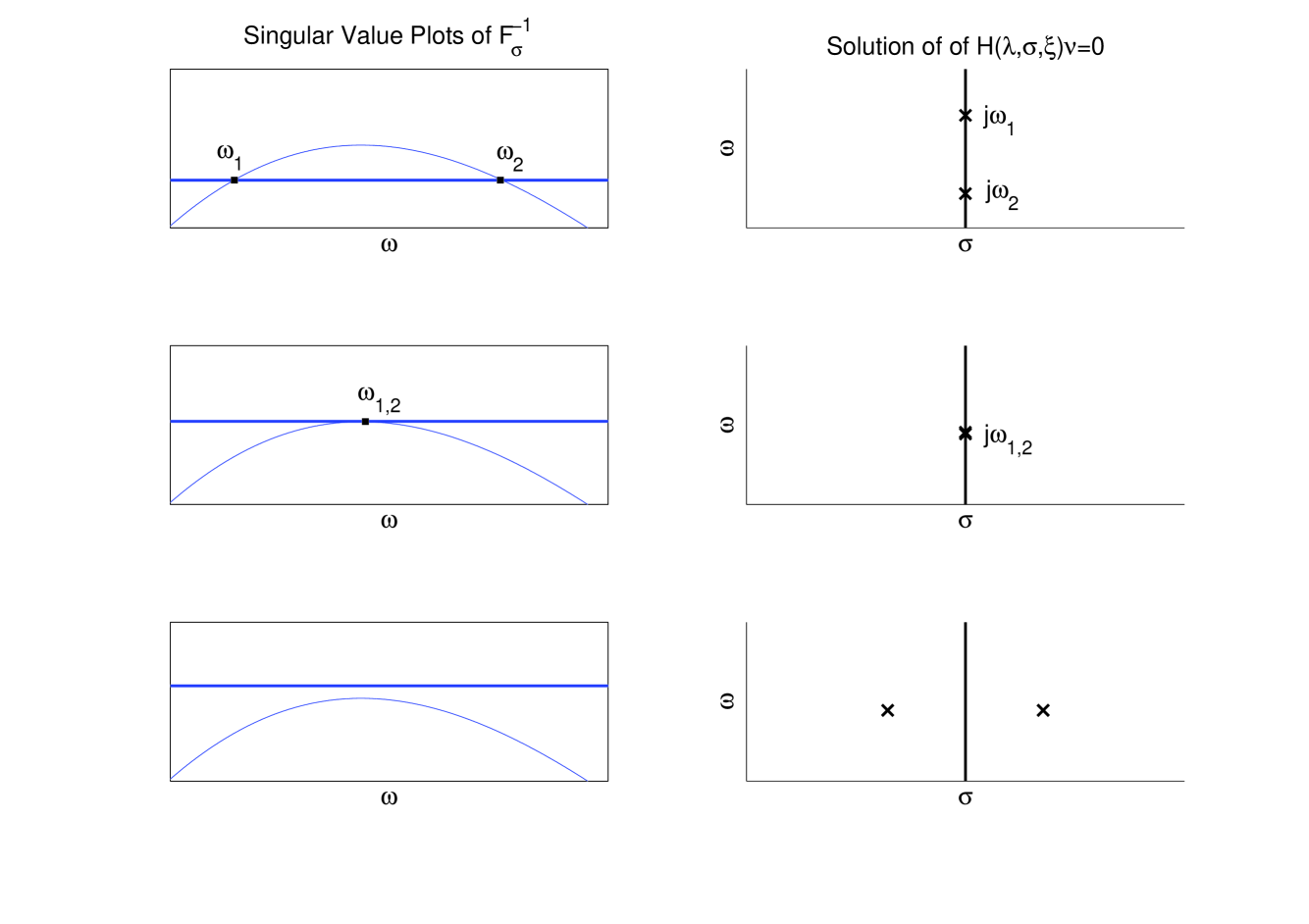
Figure 1: (left) Intersections of the singular value plot of $F_{\sigma}^{-1}$ with the horizontal line $\frac{1}{\epsilon w(\sigma)}$ for the cases where (top) $\|F_{\sigma}(j\omega)^{-1}\|_{\infty}>\frac{1}{\epsilon w(\sigma)}$, (middle) $\|F_{\sigma}^{-1}(j\omega)\|_{\infty}=\frac{1}{\epsilon w(\sigma)}$ and (bottom) $\|F_{\sigma}^{-1}(j\omega)\|_{\infty}<\frac{1}{\epsilon w(\sigma)}$. (right) Corresponding eigenvalues of the problem (45) where $\xi=\frac{1}{\epsilon w(\sigma)}$.

Let $\alpha_{\epsilon}(F)+j\omega_{\epsilon}$ be a rightmost element of $\Lambda_{\epsilon}(F)$. Setting

$$h_{\sigma}(\lambda)=\det H\left(\lambda,\sigma,\frac{1}{\epsilon w(\sigma)}\right),$$

the pair $(\omega,\sigma)=(\omega_{\epsilon},\alpha_{\epsilon}(F))$ satisfies

$$h_{\sigma}(j\omega)=0,\ \ h_{\sigma}^{\prime}(j\omega)=0.$$ (46)

These complex-valued equations seem over-determined but this is not the case due to the spectral properties of $H$, which imply the following result.

Proposition 2.

For $\omega\geq 0$, we have

$$\Im\ h_{\sigma}(j\omega)=0$$ (47)

and

$$\Re\ h_{\sigma}^{\prime}(j\omega)=0.$$ (48)

Proof.  It can easily be shown that

$$h_{\sigma}(\lambda)=h_{\sigma}(-\lambda),\ \ \ h_{\sigma}^{\prime}(\lambda)=-h_{\sigma}^{\prime}(-\lambda).$$

Substituting $\lambda=j\omega$ yields

$$\begin{array}[]{l}h_{\sigma}(j\omega)=h_{\sigma}(-j\omega)=\left(h_{\sigma}(j\omega)\right)^{*},\\ h_{\sigma}^{\prime}(j\omega)=-h_{\sigma}^{\prime}(-j\omega)=-\left(h_{\sigma}^{\prime}(j\omega)\right)^{*},\end{array}$$

and the assertions follow. $\Box$

Using Proposition 2 we can simplify the conditions (46) to:

$$\left\{\begin{array}[]{l}\Re\ h_{\sigma}(j\omega)=0,\\ \Im\ h_{\sigma}^{\prime}(j\omega)=0.\end{array}\right.$$ (49)

Hence, the pair $(\omega_{\epsilon},\alpha_{\epsilon}(F))$ can be directly computed by solving the two equations (49) for $\omega$ and $\sigma$, e.g. using Newton’s method, provided that good starting values are available.

The drawback of working directly with (49) is that an explicit expression for the determinant of $H$ is required. To avoid this, let $u,v\in\mathbb{C}^{n}$ be such that

$$H\left(j\omega,\sigma,(\epsilon w(\sigma))^{-1}\right)\left[\begin{array}[]{c}u\\ v\end{array}\right]=0,\ \ \ \hat{n}(u,v)=0,$$ (50)

where $\hat{n}(u,v)=0$ is a normalizing condition. Given the structure of $H$ it can be verified that a corresponding left eigenvector is given by $[-v^{*}\ u^{*}]$. According to [13], we get

$$h_{\sigma}^{\prime}(j\omega)=0\Leftrightarrow[-v^{*}\ u^{*}]\ \frac{\partial}{\partial\lambda}H(j\omega,\sigma,(\epsilon w(\sigma))^{-1})\left[\begin{array}[]{c}u\\ v\end{array}\right]=0.$$

A simple computation yields:

$$[-v^{*}\ u^{*}]\ \frac{\partial}{\partial\lambda}H(j\omega,\sigma,(\epsilon w(\sigma))^{-1})\left[\begin{array}[]{c}u\\ v\end{array}\right]=\\ 2\Im\left\{v^{*}\left(I+\sum_{i=1}^{m}A_{\sigma,i}\tau_{i}e^{-j\omega\tau_{i}}\right)u\right\},$$ (51)

which is always real. This is a consequence of the property (48).

Taking into account the above results, we end up with $4n+3$ real equations

$$\left\{\begin{array}[]{l}H(j\omega,\ \sigma,\ (\epsilon w(\sigma))^{-1})\left[\begin{array}[]{c}u,\\ v\end{array}\right]=0,\quad\hat{n}(u,v)=0\\ \Im\left\{v^{*}\left(I+\sum_{i=1}^{m}A_{\sigma,i}\tau_{i}e^{-j\omega\tau_{i}}\right)u\right\}=0\\ \end{array}\right.$$ (52)

in the $4n+2$ unknowns $\Re(v),\Im(v),\Re(u),\Im(u),\omega$ and $\sigma$. These equations are still overdetermined because the property (47) is not explicitly exploited in the formulation, unlike the property (48). However, it makes the equations (52) exactly solvable, and the $(\omega,\sigma)$ components have a one-to-one-correspondence with the solutions of (49).

In our implementation the equations (52) are solved using the Gauss-Newton method. This method exhibits quadratic convergence because the residual in the solution is zero, i.e., an exact solution exists [1]. The starting values are generated using the approach outlined in the previous section.

5 Algorithm

The overall algorithm for computing the pseudospectral abscissa is as follows.

Algorithm 2.

Input: system data, tolerance for prediction step, tol, and number of discretization points, $N$
Output: pseudospectral abscissa $\alpha_{\epsilon}(F)$

Prediction Step:

1. Calculate the spectral abscissa $\alpha(F_{N})$

2. $\sigma_{L}=\alpha(F_{N})$, $\sigma_{R}=\infty$, $\Delta\sigma=$tol,

3. while $(\sigma_{R}-\sigma_{L})>\textrm{tol}$

   1. if $(\sigma_{R}=\infty)$
      then $\Delta\sigma=2\times\Delta\sigma$, $\sigma_{M}=\sigma_{L}+\Delta\sigma$,
      else $\sigma_{M}=\frac{\sigma_{L}+\sigma_{R}}{2}$.

   2. if $H_{N,\sigma_{M}}$ has imaginary axis eigenvalues
      then $\sigma_{L}=\sigma_{M}$,
      else $\sigma_{R}=\sigma_{M}$.

4. {result: $\alpha_{\epsilon}^{N}(F)=\sigma_{L}$ and $j\tilde{\omega}_{i},i=1,\ldots,\tilde{n}$: imaginary axis eigenvalues of $H_{N,{\sigma}_{L}}$}

Correction Step:

1. calculate the approximate null vectors $\left\{x_{1},\ldots,x_{\tilde{n}}\right\}$ of $H(j\tilde{\omega}_{i},\alpha_{\epsilon}^{N}(F),(\epsilon w(\alpha_{\epsilon}^{N}(F)))^{-1})$ $i=1,\ldots,\tilde{n}$,

2. for all $i\in\{1,\ldots,\tilde{n}\}$, solve (52) with starting values

   $$\left[\begin{array}[]{c}u\\ v\end{array}\right]=x_{i},\ \omega=\tilde{\omega}_{i},\ \ \sigma=\alpha_{\epsilon}^{N}(F)$$

   denote the solution with $(u_{\epsilon,i},v_{\epsilon,i},\omega_{\epsilon,i},\sigma_{\epsilon,i})$.

3. set $\alpha_{\epsilon}(F):=\max_{1\leq i\leq\tilde{n}}\sigma_{\epsilon,i}$.

The two steps are the prediction step explained in Section 3 and the correction step explained in Section 4. The first step requires a repeated computation of the eigenvalues of the $2n(N+1)\times 2n(N+1)$ Hamiltonian matrix $H_{N,\sigma}$ (35). The second step solves (52), i.e. a set of $4n+3$ nonlinear equations. Our implementation chooses $N$ large enough and the tolerance in the prediction step small enough such that the results of the prediction step are good starting values for the correction step.

Note that by increasing $N$ and reducing the tolerance, the approximate pseudospectral abscissa can be computed arbitrarily close to $\alpha_{\epsilon}(F)$ by applying the prediction step only. However, this approach typically has a much larger numerical cost than the combined approach, not only because it requires a much larger value of $N$ than necessary for the corrector (to assure that $|\alpha_{\epsilon}(F)-\alpha_{\epsilon}^{N}(F)|$ sufficiently small), but also because the tolerance in the prediction step must be chosen very small (to assure that $\alpha_{\epsilon}^{N}(F)$ is computed sufficiently accurately). The latter implies that the number of iterations becomes very large. Hence, working with the prediction step only requires a much larger number of much more expensive iterations than working with the combined approach.

In our implementation, the mesh points in the approximation of $F$, discussed in Section 2, are chosen as scaled and shifted Chebyshev extremal points, i.e.,

$$\theta_{N,i}=\frac{\tau_{\max}}{2}\left(\cos\left(\frac{i\pi}{N}\right)-1\right),\ \ i=-N,\ldots,0$$ (53)

since the corresponding interpolating polynomial has less oscillation towards the end of the interval compared to choices of grid points different from (53), see [4].

Finally, we note that the prediction step is based on approximating $F$ by $F_{N}$, defined in (28), hence, on approximating the exponential functions $\lambda\mapsto\exp(-\lambda\tau_{i})$ by the rational functions $\lambda\mapsto p_{N}(-\tau_{i};\ \lambda)$. Because these approximations are essentially approximations around $\lambda=0$, our implementation incorporates the following substitution in $F(\lambda)$ to shift the center of the approximation to $\lambda=\alpha(F(\lambda))$:

$$\lambda\leftarrow\lambda+\alpha(F(\lambda)),$$

as well as a corresponding adaptation of the weights in the pseudospectrum definition. For the computation of the spectral abscissa $\alpha(F)$ we use the package DDE-BIFTOOL, [10].

6 Example

We tested the numerical method on several benchmark problems. We chose the following high-order example with many delays to give further details about the algorithm. We consider a time-delay system in (1) with the dimensions $m=7$, $n=10$ with delays $\tau_{1}=0.1$, $\tau_{2}=0.2$, $\tau_{3}=0.3$, $\tau_{4}=0.4$, $\tau_{5}=0.5$, $\tau_{6}=0.6$, $\tau_{7}=0.8$. The weights $w_{i}$ are set to $1$ and $\epsilon=0.1$. The pseudospectrum is shown with black lines and black stars indicate part of the characteristic roots of (2) in Figure 2.

Figure 2: The pseudospectrum and the pseudospectral abscissa. The stars indicate the characteristic roots of the time-delay system and the black curves are the pseudospectra contours. Vertical lines are lower and upper bounds in the bisection algorithm shown as dashed and solid lines respectively.

The tolerance in the bisection algorithm is set to $0.1$ and the discretization parameter is chosen as $N=10$. Each iteration of the while loop in the prediction step computes $\sigma_{M}$ and updates $\sigma_{L}$ or $\sigma_{R}$ shown as the vertical dashed and solid lines respectively. The approximate pseudospectral abscissa as a result of the prediction step is $\alpha_{\epsilon}^{N}(F)=-0.0525$ and the corresponding critical frequencies are $\tilde{\omega}_{1}=1.4069$, $\tilde{\omega}_{2}=1.6718$. These approximate values are improved in the correction step and the computed pseudospectral abscissa is $\alpha_{\epsilon}(F)=-0.0307$ at $\omega_{\epsilon}=1.5383$ shown as black dots in Figure 2.

In Table 1 we present the results of benchmarking of our code with $10$ time-delay plants with various perturbation sizes and perturbation weights. The second column shows the size of matrices $A_{i}$, $n$, and the number of state delays, $m$. The third column gives the minimum value of $N$ such that in the correction step the desired solution is computed. The fourth and fifth columns contain the predicted and corrected pseudospectral abscissa of the corresponding time-delay system. The last column shows the computation time for each plant in seconds on a PC with an Intel Core Duo 2.53 GHz processor with 2 GB RAM. The plant $6$ corresponds to the problem considered in this section.

Plants	$(n,m)$	$N$	$\alpha_{\epsilon}^{N}$	$\alpha_{\epsilon}$	time
$1$	$(3,1)$	$6$	$1.7784$	$1.7790$	$0.047$
$2$	$(1,1)$	$6$	$4.1497$	$4.1498$	$0.048$
$3$	$(3,3)$	$3$	$5.5034$	$5.5131$	$0.061$
$4$	$(4,9)$	$6$	$6.4172$	$6.4173$	$0.075$
$5$	$(8,20)$	$5$	$7.2918$	$7.2496$	$0.27$
$6$	$(10,7)$	$3$	$-0.02840$	$-0.03071$	$0.19$
$7$	$(20,9)$	$7$	$3.4569$	$3.4570$	$3.05$
$8$	$(40,3)$	$4$	$1.2104$	$1.2105$	$4.66$
$9^{*}$	$(5,1)$	$3$	$1.9985$	$1.9985$	$0.10$
$10^{*}$	$(4,3)$	$20$	$1.5170$	$1.5172$	$0.60$

Table 1: Benchmarks for the pseudospectral abscissa computation.

For the plant $9$ a warning is generated when using the default tolerance value of the prediction step $tol=10^{-3}$, indicating that the difference between final lower and upper bound values for the approximate pseudospectral abscissa is too large for the problem. The warning is removed when a smaller tolerance is chosen $tol=10^{-4}$. The plant $10$ gives a warning when the number of discretization points is set to the default value $N=15$. The warning is removed when $N=20$ is set. We note that both examples, plants $9$ and $10$, are difficult constructed cases. For most practical problems, the default values for the number of discretization points $N=15$ and the tolerance of the prediction step $tol=10^{-3}$ is sufficient.

The problem data for the above benchmark examples (system matrices $A_{i}$, state delays $\tau_{i}$, perturbation weights $w_{i}$ for $i=0,\ldots,m$, the perturbation size $\epsilon$ and options if necessary) and a MATLAB implementation of our code for the pseudospectral abscissa computation are available at the website

http://www.cs.kuleuven.be/~wimm/software/psa/

7 Concluding Remarks

An accurate method to compute the pseudospectral abscissa of retarded time-delay systems with an arbitrary number of delays is given. The method is based on two steps: the prediction step calculates an approximation of the pseudospectral abscissa based on a finite-dimensional approximation of the problem. The correction step computes the pseudospectral abscissa by solving nonlinear equations that characterize the rightmost points of the pseudospectrum. The method has been successfully applied to benchmark problems demonstrating its effectiveness.

After the pseudospectral abscissa of the time-delay plant is computed, the gradient of the pseudospectral abscissa with respect to system matrices and delays can be calculated for the complex point where pseudospectral abscissa is achieved. By embedding the pseudospectral abscissa computation in an optimization loop, a fixed structure controller minimizing the pseudospectral abscissa can be designed inspired by the approach of [12] for the finite dimensional case. This is our future research direction.

This article present results of the Belgian Programme on Interuniversity Poles of Attraction, initiated by the Belgian State, Prime Minister’s Office for Science, Technology and Culture, and of OPTEC, the Optimization in Engineering Centre of the K.U.Leuven.

Appendix A Proof of Theorem 2.2

We need the following proposition to prove the Theorem 2.2.

Proposition A.1.

We can express

$$p_{N}(-\tau_{i};\ \lambda)=\frac{r_{i}(\lambda)}{s(\lambda)},\ 1=1,\ldots,m,$$ (54)

where $s$ is a monic polynomial of degree $N$ and $r_{i},\ i=1,\ldots,m$ are polynomials of degree smaller than or equal to $N$. Furthermore, we have

$$s(\lambda)=\det(\lambda I-D_{1,1})$$ (55)

and

$$\left[\begin{array}[]{c}p_{N}(\theta_{N,-N};\ \lambda)\\ \vdots\\ p_{N}(\theta_{N,-1};\ \lambda)\end{array}\right]=(\lambda I-D_{1,1})^{-1}D_{1,2}.$$ (56)

where $D_{1,1}$ and $D_{1,2}$ are given in (22).

Proof.  In a Lagrange basis we can express

$$p_{N}(t;\ \lambda)=\sum_{i=-N}^{0}c_{i}l_{N,i}(t),$$

where, for the simplicity of the notations, we suppress the dependence of the coefficients $c_{i}$ on $\lambda$. The conditions (26) can be expressed as $c_{0}=1$ and

$$(\lambda I-D_{1,1})\left[\begin{array}[]{l}c_{-N}\\ \vdots\\ c_{-1}\end{array}\right]=D_{1,2},$$

which implies that

$$p_{N}(t;\ \lambda)=l_{N,0}(t)+[l_{N,-N}(t)\ \cdots\ l_{N,-1}](\lambda I-D_{1,1})^{-1}D_{1,2}.$$

The assertions follow. $\Box$

Proof of Theorem 2.2.  Using the formula for the determinant of a two-by-two block matrix based on Schur complements and with ${\bf A_{N}}$ and $D$ given in (25) and (22) respectively, it follows that

$$\det(\lambda I-{\bf A_{N}})=\det((\lambda I_{N}-D_{1,1})\otimes I_{n})\det(\lambda I_{n}-\Gamma_{0}\\ -[\Gamma_{-N}\cdots\Gamma_{-1}]((\lambda I_{N}-D_{1,1})\otimes I_{n})^{-1}(D_{1,2}\otimes I_{n})),$$ (57)

$$=s(\lambda)^{n}\det\left(\lambda I_{n}-\Gamma_{0}-\sum_{i=-N}^{-1}\Gamma_{i}I_{n}\ p_{N}(\theta_{N,i};\ \lambda)\right),$$

$$=s(\lambda)^{n}\det\left(\lambda I_{n}-A_{0}\right.\\ \left.-\sum_{i=-N}^{0}\sum_{l=1}^{m}A_{l}l_{N,i}(-\tau_{l})p_{N}(\theta_{N,i};\ \lambda)\right),$$ (58)

$$=s(\lambda)^{n}\det\left(\lambda I_{n}-A_{0}-\sum_{l=1}^{m}A_{l}\right.\\ \left.\sum_{i=-N}^{0}l_{N,i}(-\tau_{l})p_{N}(\theta_{N,i};\ \lambda)\right),$$ (59)

$$=s(\lambda)^{n}\det\left(\lambda I_{n}-A_{0}-\sum_{l=1}^{m}A_{l}p_{N}(-\tau_{l};\ \lambda)\right).$$ (60)

Furthermore, using the same approach, we can derive for $k,l\in\{1,\ldots,n\}$:

$$\Delta^{k,l}_{N}(\lambda):=\left\{{\bf B_{N}}^{*}\ \mathrm{adj}(\lambda I_{(N+1)n}-{\bf A_{N}}){\bf B_{N}}\right\}_{k,l},\\ =\det((\lambda I_{N}-D_{1,1})\otimes I_{n})\det(\lambda\tilde{I}_{n-1}-\tilde{\Gamma}_{0}-[\tilde{\Gamma}_{-N}\cdots\tilde{\Gamma}_{-1}]\\ ((\lambda I_{N}-D_{1,1})\otimes I_{n})^{-1}(D_{1,2}\otimes\tilde{I}_{n})),$$ (61)

where the superscript ~ denotes that an appropriate row and/or column have been removed. Using Proposition A.1 and following the steps in (60), this expression can be written as

$$\begin{array}[]{l}\Delta_{N}^{k,l}(\lambda)=s(\lambda)^{n}\det\left(\lambda\tilde{I}-\tilde{\Gamma}_{0}-\sum_{i=-N}^{-1}\tilde{\Gamma}_{i}\tilde{I}\ p_{N}(\theta_{N,i};\ \lambda)\right)\\ =s(\lambda)^{n}\left\{\mathrm{adj}\left(\lambda I-A_{0}-\sum_{l=1}^{m}A_{l}\ p_{N}(-\tau_{l};\ \lambda)\right)\right\}_{k,l}.\end{array}$$ (62)

Using (60)-(62) we can derive:

$$\begin{array}[]{l}{\bf B_{N}}^{T}(\lambda I-{\bf A_{N}})^{-1}{\bf B_{N}}={\bf B_{N}}^{T}\frac{\mathrm{adj}(\lambda I-{\bf A_{N}})}{\det(\lambda I-{\bf A_{N}})}{\bf B_{N}}\\ =\frac{\mathrm{adj}\left(\lambda I-A_{0}-\sum_{i=1}^{m}A_{i}p_{N}(-\tau_{i};\ \lambda)\right)}{\det\left(\lambda I-A_{0}-\sum_{i=1}^{m}A_{i}p_{N}(-\tau_{i};\ \lambda)\right)}\\ =(\lambda I-A_{0}-\sum_{i=1}^{m}A_{i}p_{N}(-\tau_{i};\ \lambda))^{-1}.\end{array}$$

This completes the proof. $\Box$

References

• [1] A. Björck. Numerical methods for least squares problems. SIAM, 1996.
• [2] S. Boyd, V. Balakrishnan, and P. Kabamba. A bisection method for computing the $\mathcal{H}_{\infty}$-norm of a transfer matrix and related problems. Mathematics of Control, Signals, and Systems, 2:207–219, 1989.
• [3] D. Breda, S. Maset, and R. Vermiglio. Pseudospectral differencing methods for characteristic roots of delay differential equations. SIAM Journal on Scientific Computing, 27:482–495, 2005.
• [4] D. Breda, S. Maset, and R. Vermiglio. Pseudospectral approximation of eigenvalues of derivative operators with non-local boundary conditions. Applied Numerical Mathematics, 56:318–331, 2006.
• [5] J.V. Burke, A.S. Lewis, and M.L. Overton. Optimization and pseudospectra, with applications to robust stability. SIAM Journal on Matrix Analysis and Applications, 25:80–104, 2003.
• [6] J.V. Burke, A.S. Lewis, and M.L. Overton. Robust stability and a criss-cross algorithm for pseudospectra. IMA Journal of Numerical Analysis, 23:359–375, 2003.
• [7] R. Byers. A bisection method for measuring the distance of a stable matrix to the unstable matrices. SIAM Journal on Scientific and Statistical Computing, 9:875–881, 1988.
• [8] DQ Cao, P He, and K Zhang. Exponential stability criteria of uncertain systems with multiple time delays. Journal Of Mathematical Analysis And Applications, 283(2):362–374, 2003.
• [9] R. Curtain and H. Zwart. An Introduction to Infinite-Dimensional Linear Systems Theory. Texts In Applied Mathematics vol. 21, Springer, 1995.
• [10] K. Engelborghs, T. Luzyanina, and D. Roose. Numerical bifurcation analysis of delay differential equations using dde-biftool. ACM Transactions on Mathematical Software, 28:1–21, 2002.
• [11] Y. Genin, R. Stefan, and P. Van Dooren. Real and complex stability radii of polynomial matrices. Linear Algebra and its Applications, 351-352:381–410, 2002.
• [12] Suat Gumussoy, Didier Henrion, M. Millstone, and M.L. Overton. Multiobjective robust control with hifoo 2.0. In Proceedings of the 6th IFAC Symposium on Robust Control Design, 2009.
• [13] R. Hryniv and P. Lancaster. On the perturbation of analytic matrix functions. Integral Equations and Operator Theory, 34:325–338, 1999.
• [14] V Kharitonov, J Collado, and S Mondie. Exponential estimates for neutral time delay systems with multiple delays. International Journal Of Robust And Nonlinear Control, 16(2):71–84, 2006.
• [15] W. Michiels, K. Green, T. Wagenknecht, and S.-I. Niculescu. Pseudospectra and stability radii for analytic matrix functions with application to time-delay systems. Linear Algebra and its Applications, 418:315–335, 2006.
• [16] W. Michiels and S.-I. Niculescu. Stability and Stabilization of Time-Delay Systems. An Eigenvalue Based Approach. SIAM, 2007.
• [17] Zhan Shu, James Lam, and Shengyuan Xu. Improved exponential estimates for neutral systems. Asian Journal Of Control, 11(3):261–270, 2009.
• [18] L. Trefethen. Pseudospectra of linear operators. SIAM Review, 39:383–406, 1997.
• [19] WJ Wang and RJ Wang. Robust stability for noncommensurate time-delay systems. IEEE Transactions On Circuits And Systems I-Fundamental Theory And Applications, 45(4):507–511, 1998.