CAFENet: Class-Agnostic Few-Shot
Edge Detection Network

Abstract

We tackle a novel few-shot learning challenge, which we call few-shot semantic edge detection, aiming to localize crisp boundaries of novel categories using only a few labeled samples. We also present a Class-Agnostic Few-shot Edge detection Network (CAFENet) based on meta-learning strategy. CAFENet employs a semantic segmentation module in small-scale to compensate for lack of semantic information in edge labels. The predicted segmentation mask is used to generate an attention map to highlight the target object region, and make the decoder module concentrate on that region. We also propose a new regularization method based on multi-split matching. In meta-training, the metric-learning problem with high-dimensional vectors are divided into small subproblems with low-dimensional sub-vectors. Since there is no existing dataset for few-shot semantic edge detection, we construct two new datasets, FSE-1000 and SBD-$5^{i}$, and evaluate the performance of the proposed CAFENet on them. Extensive simulation results confirm the performance merits of the techniques adopted in CAFENet.

ew-shot edge detection, few-shot learning, semantic edge detection

1 Introduction

Semantic edge detection aims to identify pixels that belong to boundaries of predefined categories. It is shown that semantic edge detection is useful for a variety of computer vision tasks such as semantic segmentation [3, 5, 6, 8, 55], object reconstruction [14, 46, 59], image generation [25, 49] and medical imaging [1, 36]. Early edge detection algorithms interpret the problem as a low-level grouping problem exploiting hand-crafted features and local information [7, 19, 44]. Recently, there have been significant improvements on edge detection thanks to the advances in deep learning [4, 21, 24, 51]. Moreover, beyond previous boundary detection, category-aware semantic edge detection became possible [2, 23, 54, 56]. However, it is impossible to train deep neural networks without massive amounts of annotated data.

To overcome the data scarcity issue in image classification, few-shot learning has been actively discussed for recent years [16, 31, 43, 47]. Few-shot learning algorithms train machines to learn previously unseen classification tasks using only a few relevant labeled examples. More recently, the idea of few-shot learning is applied to computer vision tasks requiring highly laborious and expensive data labeling such as semantic segmentation [12, 42, 48] and object detection [17, 26, 27]. Based on meta-learning across varying tasks, the machines can adapt to unencountered environments and demonstrate robust performance in various computer vision problems. In this paper, we consider a novel few-shot learning challenge, few-shot semantic edge detection, to detect the semantic boundaries using only a few labeled samples. To tackle this elusive challenge, we also propose a class-agnostic few-shot edge detector (CAFENet) and present new datasets for evaluating few-shot semantic edge detection.

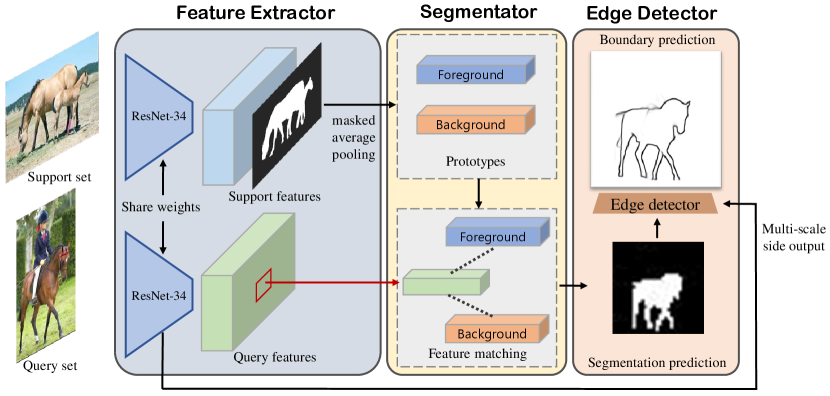
Figure 1: Architecture overview of the proposed CAFENet. The feature extractor or encoder extracts feature from the image, the segmentator generates a segmentation mask based on metric learning, and the edge detector detects semantic boundaries using the segmentation mask and query features.

Fig. 1 shows the architecture of the proposed CAFENet. Since the edge labels do not contain enough semantic information due to the sparsity of labels, performance of the edge detector severely degrades when the training dataset is very small. To overcome this, we adopt the segmentation process in advance of detecting edge with downsized feature and segmentation labels generated from boundaries labels. We utilize a simple metric-based segmentator generating a segmentation mask through pixel-wise non-parametric feature matching with class prototypes, which are computed by masked average pooling of [58]. The predicted segmentation mask provides the semantic information to the edge detector. The multi-scale attention maps are generated from the segmentation mask, and applied to corresponding multi-scale features. The edge detector predicts the semantic boundaries using the attended features. Using this attention mechanism, the edge detector can focus on relevant regions while alleviating the noise effect of external details.

For meta-training of CAFENet, we introduce a simple yet powerful regularization method, Multi-Split Matching Regularization (MSMR), performing metric learning on multiple low-dimensional embedding sub-spaces. During meta-training, the model is meta-learned to minimize distances between the pixels of query features and the prototype of same class for segmentation. At the same time, the prototypes and pixels of feature vectors are divided into multiple low-dimensional splits and the model also learns to minimize distances between the pixels of query feature splits and their corresponding prototype splits of the same class. The proposed MSMR method can achieve significant performance gain without additional learnable parameters.

To sum up, the main contributions of this paper are as follows:

$\bullet$ 

We introduce the few-shot semantic edge detection problem for performing semantic edge detection on previously unseen objects using only a few training examples.

$\bullet$ 

We propose to generate an attention map using a segmentation prediction mask and attend convolutional features so as to localize semantically important regions prior to edge detection.

$\bullet$ 

We introduce a novel MSMR regularization method dividing high-dimensional vectors into low-dimensional sub-vectors and conduct metric-learning sub-problems for few-shot semantic edge detection.

$\bullet$ 

We introduce two datasets for few-shot semantic edge detection and validate the proposed CAFENet techniques.

2 Related Work

2.1 Few-shot Learning

To tackle the few-shot learning challenge, many methods have been proposed based on meta-learning. Optimization-based methods [16, 40, 41] train the meta-learner which updates the parameters of the actual learner so that the learner can easily adapt to a new task within a few labeled samples. Metric-based methods [15, 29, 43, 45, 47, 52] train the feature extractor to assemble features from the same class together on the embedding space while keeping features from different classes far apart. Recent metric-based approaches propose dense classification [22, 30, 31, 38]. Dense classification trains an instance-wise classifier on pixel-wise classification loss which imposes coherent predictions over the spatial dimension and prevents overfitting as a result. Our model adopts the metric-based method for few-shot learning. Inspired by dense classification, we propose multi-split matching regularization which divides the feature vector into sub-vector splits and performs split-wise classification for regularization in meta-learning

2.2 Few-shot Semantic Segmentation

The goal of few-shot segmentation is to perform semantic segmentation within a few labeled samples based on meta-learning [12, 39, 42, 48, 57]. OSLSM of [42] adopts a two-branch structure: conditioning branch generating element-wise scale and shift factor using the support set and segmentation branch performing segmentation with a fully convolutional network and task-conditioned features. Co-FCN [39] also utilizes a two-branch structure. The globally pooled prediction is generated using support set in conditioning branch, and fused with query features to predict segmentation mask in segmentation branch. SG-One of [58] proposes a masked average pooling to compute prototypes from pixels of support features. The cosine similarity scores are computed between the prototypes and pixels of query feature, and the similarity map guides the segmentation process. CANet of [57] also adopts masked average pooling to generate the global feature vector, and concatenate it with every location of the query feature for dense comparison in predicting the segmentation mask. PANet of [48] introduces prototype alignment for regularization, to predict the segmentation mask of support samples using query prediction results as labels of query samples.

2.3 Semantic Edge Detection

Semantic edge detection aims to find the boundaries of objects from image and classify the objects at the same time. The history of semantic edge detection [2, 20, 23, 33, 37, 54, 56] dates back to the work of [37] which adopts the support vector machine as a semantic classifier on top of the traditional canny edge detector. Recently, many semantic edge detection algorithms rely on deep neural network and multi-scale feature fusion. CASENET of [54] addresses the semantic edge detection as a multi-label problem where each boundary pixel is labeled into categories of adjacent objects. Dynamic Feature Fusion (DFF) of [23] proposes a novel way to leverage multi-scale features. The multi-scale features are fused by weighted summation with fusion weights generated dynamically for each images and each pixel. Meanwhile, Simultaneous Edge Alignment and Learning (SEAL) of [56] deals with severe annotation noise of the existing edge dataset [20]. SEAL treats edge labels as latent variables and jointly trains them to align noisy misaligned boundary annotations. Semantically Thinned Edge Alignment Learning (STEAL) of [2] improves the computation efficiency of edge label alignment through a lightweight level set formulation. In addition, STEAL optimizes the model for non-maximum suppression (NMS) during training while previous works use NMS at the postprocessing step.

3 Problem Setup

For few-shot semantic edge detection, we use train set $D_{train}$ and test set $D_{test}$ consisting of non-overlapping categories $C_{train}$ and $C_{test}$. The model is trained only using $C_{train}$, and the test categories $C_{test}$ are never seen during the training phase. For meta-training of the model, we adopt episodic training as done in many previous few-shot learning works. Each episode is composed of a support set with a few-labeled samples and a query set. When an episode is given, the model adapts to the given episode using the support set and detect semantic boundaries of the query set. By episodic training, the model is learned so that it adapts to the unseen class using only a few labeled samples and predict semantic edges of query samples.

For $N_{c}$-way $N_{s}$-shot setting, each training episode is constructed by $N_{c}$ classes sampled from $C_{train}$. When $N_{c}$ categories are given, $N_{s}$ support samples and $N_{q}$ query samples are randomly chosen from $D_{train}$ for each class. In evaluation, the performance of the model is evaluated using test episodes. The test episodes are constructed in the same way as the training episodes, except $N_{c}$ classes and corresponding support and query samples are sampled from $C_{test}$ and $D_{test}$.

In this work, we address $N_{c}$-way $N_{s}$-shot semantic edge detection. The goal is training the model to generalize to $N_{c}$ unseen classes given only $N_{s}$ images and their edge labels. Based on the few labeled support samples, the model should produce edge predictions of query images which belong to $N_{c}$ unencountered classes.

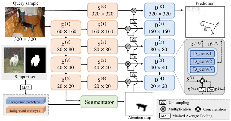
Figure 2: Network architecture overview of proposed CAFENet. ResNet-34 encoder $E^{(1)}\sim E^{(4)}$ extracts multi-level semantic features. The segmentator module generates a segmentation prediction using query feature from $E^{(4)}$ and prototypes $P_{FG},P_{BG}$ from support set features. Small bottleneck blocks ${S}^{(0)}\sim{S}^{(4)}$ transform the original image and multi-scale features from encoder blocks to be more suitable for edge detection. The attention maps generated from segmentation prediction are applied to multi-scale features to localize the semantically related region. Decoder $D^{(0)}\sim D^{(4)}$ takes attentive multi-scale features to give edge prediction.

4 Method

We propose a novel algorithm for few-shot semantic edge detection. Fig. 2 illustrates the network architecture of the proposed method. The proposed CAFENet adopts the semantic segmentation module to compensate for the lack of semantic information in edge labels. The predicted segmentation mask is utilized for attention in skip connection. The final edge detection is done using attentive multi-scale features.

4.1 Semantic Segmentator

Most previous works on semantic edge detection directly predict edges from the given input image. However, direct edge prediction is a hard task when only a few labeled samples are given. To overcome this difficulty in few-shot edge detection, we adopt a semantic segmentation module in advance of edge prediction. With the assistance of the segmentation module, CAFENet can effectively localize the target object and extract semantic features from query samples. For few-shot segmentation, we employ the metric-learning which utilizes prototypes for foreground and background as done in [12, 48]. Given the support set $S=\{x^{s}_{i},y^{s}_{i}\}^{N_{s}}_{i=1}$, the encoder $E$ extracts features $\{E(x^{s}_{i})\}^{N_{s}}_{i=1}$ from $S$. Also, for support labels $\{y^{s}_{i}\}^{N_{s}}_{i=1}$, we generate the dense segmentation mask $\{M^{s}_{i}\}^{N_{s}}_{i=1}$ using a rule-based preprocessor, considering the pixels inside the boundary as foreground pixels in the segmentation label. Using down-sampled segmentation labels $\{m^{s}_{i}\}^{N_{s}}_{i=1}$, the prototype for foreground pixels $P_{FG}$ is computed as

$$P_{FG}=\frac{1}{N_{s}}\frac{1}{H\times{W}}\sum_{i}\sum_{j}E_{j}(x^{s}_{i})m^{s}_{i,j}$$ (1)

where $j$ indexes the pixel location, $E_{j}(x)$ and $m^{s}_{i,j}$ denote the $j$th pixel of feature $E(x)$ and segmentation mask $m^{s}_{i}$. $H,W$ denote height and width of the images. Likewise, the background prototype $P_{BG}$ is computed as

$$P_{BG}=\frac{1}{N_{s}}\frac{1}{H\times{W}}\sum_{i}\sum_{j}E_{j}(x^{s}_{i})(1-m^{s}_{i,j}).$$ (2)

Following the prototypical networks of [43], the probability that pixel $j$ belongs to foreground for the query sample $x^{q}_{i}$ is

$$p(y_{i,j}^{q}=FG|x^{q}_{i};E)=\frac{exp(-\tau d(E_{j}(x^{q}_{i}),P_{FG}))}{exp(-\tau d(E_{j}(x^{q}_{i}),P_{FG}))+exp(-\tau d(E_{j}(x^{q}_{i}),P_{BG}))}$$ (3)

where $d(\cdot,\cdot)$ is squared Euclidean distance between two vectors and $\tau$ is a learnable temperature parameter used in [18, 38]. With query samples $\{x^{q}_{i}\}^{N_{q}}_{i=1}$ and the down-sampled segmentation labels for query $\{m^{q}_{i}\}^{N_{q}}_{i=1}$, the segmentation loss $L_{Seg}$ is calculated as the mean-squared error (MSE) loss between predicted probabilities and the down-sized segmentation mask

$$L_{Seg}=\frac{1}{N_{q}}\frac{1}{H\times{W}}\sum_{i=1}^{N_{q}}\sum_{j=1}^{H\times{W}}\{(p(y_{i,j}^{q}=FG|x^{q}_{i};E)-m_{i,j}^{q})^{2}\}.$$ (4)

Note that the segmentation mask is generated in down-sized scale so that any pixel near the boundaries can be classified into the foreground to some extent, as well as the background. Therefore, we approach the problem as a regression using MSE loss rather than cross entropy loss.

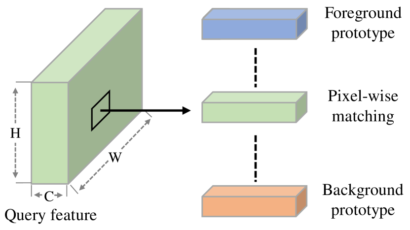
(a) High-dimensional Matching

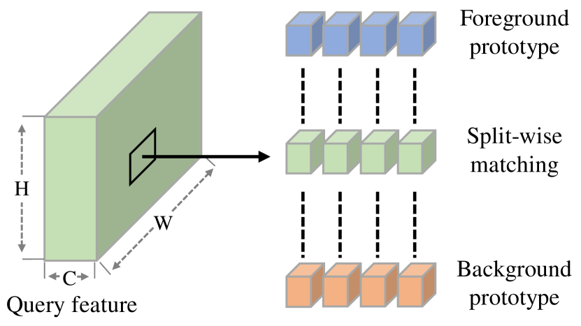
(b) Split-wise Matching

Figure 3: Comparison between (a) High-dimensional feature matching used in [12, 48] and (b) split-wise feature matching in MSMR

4.2 Multi-Split Matching Regularization

The metric-based few-shot segmentation method utilizes distance metrics between the high-dimensional feature vectors and prototypes, as seen in Fig. 3(a). However, this approach is prone to overfit due to the massive number of parameters in feature vectors. To get around this issue, we propose a novel regularization method, multi-split matching regularization (MSMR). MSMR inherits the spirit of dense feature matching [30] where pixel-wise feature matching acts as a regularizer for high-dimensional embedding. In MSMR, high-dimensional feature vectors are split into several low-dimensional feature vectors, and the metric learning is conducted on each vector split as Fig. 3(b).

With the query feature $E(x_{i}^{q})\in\mathbb{R}^{C\times{W}\times{H}}$, where $C$ is channel dimension and $H,W$ are spatial dimensions, we divide $E(x_{i}^{q})$ into $K$ sub-vectors $\{E^{k}(x_{i}^{q})\}^{K}_{k=1}$ along channel dimension. Each sub-vector $E^{k}(x_{i}^{q})$ is in $\mathbb{R}^{\frac{C}{K}\times{W}\times{H}}$. Likewise, the prototypes $P_{FG}$ and $P_{BG}$ are also disassembled into $K$ sub-vectors $\{P^{k}_{FG}\}^{K}_{k=1}$ and $\{P^{k}_{BG}\}^{K}_{k=1}$ along channel dimension where $P^{k}_{FG},P^{k}_{BG}\in{\mathbb{R}^{\frac{C}{K}}}$ . For the $k^{th}$ sub-vector of query feature $E^{k}(x_{i}^{q})$, the probability that the $j^{th}$ pixel belongs to the foreground class is computed as follows:

$$p^{k}(y_{i,j}^{q}=FG|x_{i}^{q};E)=\frac{exp(-\tau d(E_{j}^{k}(x^{q}_{i}),P^{k}_{FG}))}{exp(-\tau d(E_{j}^{k}(x^{q}_{i}),P^{k}_{FG}))+exp(-\tau d(E_{j}^{k}(x^{q}_{i}),P^{k}_{BG}))}.$$ (5)

Multi-split matching regularization divides the original metric learning problem into $K$ small sub-problems composed of a fewer parameters and acts as regularizer for high-dimensional embeddings. The prediction results of $K$ sub-problems are reflected on learning by combining the split-wise segmentation losses to original segmentation loss in Eq.(4). The total segmentation loss is calculated as

$$L_{Seg}=\frac{1}{N_{q}}\frac{1}{H\times{W}}\sum_{i=1}^{N_{q}}\sum_{j=1}^{H\times{W}}\{(p_{i,j}-m_{i,j}^{q})^{2}+\sum_{i=1}^{K}(p^{k}_{i,j}-m_{i,j}^{q})^{2}\}.$$ (6)

where $p_{i,j}=p(y_{i,j}^{q}=FG|x^{q}_{i};E)$ and $p^{k}_{i,j}=p^{k}(y_{i,j}^{q}=FG|x^{q}_{i};E)$.

4.3 Attentive Edge Detector

As shown in Fig. 2, we adopt the nested encoder structure of [34, 51] to extract rich hierarchical features. The multi-scale side outputs from encoder $E^{(1)}\sim E^{(4)}$ are post-processed through bottleneck blocks $S^{(1)}\sim S^{(4)}$. Since ResNet-34 gives side outputs of down-sized scale, we pass the original image through bottleneck block $S^{(0)}$ to extract local details in original scale. In front of $S^{(3)}$, we employ the Atrous Spatial Pyramid Pooling (ASPP) block of [9]. We have empirically found that locating ASPP there shows better performance.

In utilizing multi-scale features, we employ the predicted segmentation mask $\hat{M}$ from the segmentator where the $j^{th}$ pixel of $\hat{M}$ is the predicted probability from Eq. (3). Note that we generate $\hat{M}$ based on the entire feature vectors and the prototypes instead of utilizing sub-vectors, since the split-wise metric learning is used only for regularizing the segmentation module. For each layer $l$, $\hat{M}^{(l)}$ denotes the segmentation mask upscaled to the corresponding feature size by bilinear interpolation. Using segmentation prediction mask $\hat{M}^{(l)}$, we generate attention map $A^{(l)}$, as follows. First, the prediction with a value lower than threshold $\lambda$ is rounded down to zero, to ignore activation in regions with low confidence. Second, we broaden the attention map using morphological dilation of [13] as a second chance, since the segmentation module may not always guarantee fine results. The final attention map of $l^{th}$ layer $A^{(l)}$ is computed as follows

$$A^{(l)}=\mathds{1}(\hat{M}^{(l)}>\lambda){\hat{M}}^{(l)}+Dilation(\mathds{1}(\hat{M}^{(l)}>\lambda){\hat{M}}^{(l)})$$ (7)

where $\mathds{1}(\hat{M}^{(l)}>\lambda){\hat{M}}^{(l)}$ is the rounded value of prediction mask $\hat{M}^{(l)}$. The attention maps are applied to the multi-scale features of corresponding bottleneck blocks $S^{(0)}\sim S^{(4)}$. We apply the residual attention of [22], where the initial multi-level side outputs from $S^{(l)}$ are pixel-wisely weighted by $1+A^{(l)}$, to strengthen the activation value of the semantically important region. We visualize the effect of semantic attention in Fig. 4.

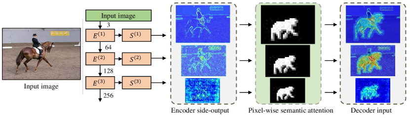
Figure 4: An example of activation map of [53] before and after pixel-wise semantic attention (warmer color has higher value). As seen, the attention mechanism makes encoder side-outputs attend to the regions of the target object (horse in the figure).

As shown in Fig. 2, the decoder network is composed of five consecutive convolutional blocks. Each decoder block $D^{(l)}$ contains three $3\times{3}$ convolution layers. The outputs of decoder blocks $D^{(1)}\sim D^{(4)}$ are bilinearly upsampled by two and passed to the next block. Similar to [13], the up-sampled decoder outputs are then concatenated to the skip connection features from bottleneck blocks $S^{(0)}\sim S^{(4)}$ and previous decoder blocks. Multi-scale semantic information and local details are transmitted through skip architectures. The hierarchical decoder network in turn refines the outputs of the previous decoder blocks and finally produces the edge prediction $\hat{y}^{q}_{i}$ of query samples $x^{q}_{i}$.

Following the work of [11], we combine cross-entropy loss and Dice loss to produce crisp boundaries. Given a query set $Q=\{x^{q}_{i},y^{q}_{i}\}^{N_{q}}_{i=1}$ and prediction mask $\hat{y}^{q}_{i}$, the cross-entropy loss is computed as

$$L_{CE}=-\sum_{i=1}^{N_{q}}\{\sum_{j\in Y_{+}}log(\hat{y}^{q}_{i})+\sum_{j\in Y_{-}}log(1-\hat{y}^{q}_{i})\}$$ (8)

where $Y_{+}$ and $Y_{-}$ denote the sets of foreground and background pixels. The Dice loss is then computed as

$$L_{Dice}=\sum_{i=1}^{N_{q}}\{\frac{\sum_{j}(\hat{y}^{q}_{i,j})^{2}+\sum_{j}({y}^{q}_{i,j})^{2}}{2\sum_{j}\hat{y}^{q}_{i,j}{y}^{q}_{i,j}}\}$$ (9)

where j denotes the pixels of a label. The final loss for meta-training is given by

$$L_{final}=L_{Seg}+L_{CE}+L_{Dice}.$$ (10)

5 Experiments

5.1 Datasets

5.1.1 FSE-1000

The datasets used in previous semantic edge detection research such as SBD of [20] and Cityscapes of [10] are not suitable for few-shot learning as they have only 20 and 30 classes, respectively. We propose a new dataset for few-shot edge detection, which we call FSE-1000, based on FSS-1000 of [50]. FSS-1000 is a dataset for few-shot segmentation and composed of 1000 classes and 10 images per class with foreground-background segmentation annotation. From the images and segmentation masks of FSS-1000, we build FSE-1000 by extracting boundary labels from segmentation masks. In the light of difficulty associated with few-shot setting, we extract thick edges of which thickness is around 2 $\sim$ 3 pixels on average. For dataset split, we split 1000 classes into 800 training classes and 200 test classes. We will provide the detailed class configuration in the Supplementary Material.

Figure 5: Qualitative examples of 5-shot edge detection on FSE-1000 dataset.

5.1.2 SBD-$5^{i}$

Based on the SBD dataset of [20] for semantic edge detection, we propose a new SBD-$5^{i}$ dataset. With reference to the setting of Pascal-$5^{i}$, 20 classes of the SBD dataset are divided into 4 splits. In the experiment with split $i$, 5 classes in the $i$th split are used as test classes $C_{test}$. The remaining 15 classes are utilized as training classes $C_{train}$. The training set $D_{train}$ is constructed with all image-annotation pairs whose annotation include at least one pixel from the classes in $C_{train}$. For each class, the boundary pixels which do not belong to that class are considered as background. The test set $D_{test}$ is also constructed in the same way as $D_{train}$, using $C_{test}$ this time. Considering the difficulty of few-shot setting and severe annotation noise of the SBD dataset, we extract thicker edges as done in FSE-1000. We utilize edges extracted from the segmentation mask as ground truth instead of original boundary labels of the SBD dataset, and thickness of extracted edge lies between $3\sim 4$ pixels on average. We conduct 4 experiments with each split of $i=0\sim 3$, and report performance of each split as well as the averaged performance. Note that unlike Pascal-$5^{i}$, we do not consider division of training and test samples of the original SBD dataset. As a result, the images in $D_{train}$ might appear in $D_{test}$ with different annotation from class in $C_{test}$.

Figure 6: Qualitative examples of 5-shot edge detection on SBD-$5^{i}$ dataset.

5.2 Evaluation Settings

We use two evaluation metrics to measure the few-shot semantic edge detection performance of our approach: the Average Precision (AP) and the maximum F-measure (MF) at optimal dataset scale(ODS).

In evaluation, we compare the unthinned raw prediction results and the ground truths without Non-Maximum Suppression (NMS) following [2, 56]. For the evaluation of edge detection, an important parameter is matching distance tolerance which is an error threshold between the prediction result and the ground truth. Prior works on edge detection such as [2, 20, 54, 56] adopt non-zero distance tolerance to resolve the annotation noise of edge detection datasets. However, the proposed datasets for few-shot edge detection utilize thicker boundaries to overcome the annotation noise issue instead of adopting distance tolerance. Moreover, evaluation with non-zero distance tolerance requires additional heavy computation. This becomes more problematic under few-shot setting where the performance should be measured on the same test image multiple times due to the variation in the support set. For these reasons, we set distance tolerance to be 0 for both FSE-1000 and SBD-$5^{i}$. In addition, we evaluate the positive predictions from the area inside an object and zero-padded region as false positives, which is stricter than the evaluation protocol in prior works of [20, 54].

5.3 Implementation Detail

We implement our framework using Pytorch library and adopt Scikit-learn library to construct the precision-recall curve and compute average precision (AP). For the encoder, ResNet-34 pretrained on ImageNet is adopted. All parameters except the encoder parameters are learned from scratch. The entire network is trained using the Adam optimizer of [28] with weight decay regularization of [35]. In both experiments on FSE-1000 and SBD-$5^{i}$, we use a learning rate of $10^{-4}$ and an $l2$ weight decay rate of $10^{-2}$. For FSE-1000 experiments, the model is trained with 40,000 episodes and the learning rate is decayed by 0.1 after training 38,000 episodes. For SBD-$5^{i}$ experiments, 30,000 episodes are used for training, and the learning rate is decayed by 0.1 after training 28,000 episodes. Higher shot training of [32] is employed in 1-shot experiments for both datasets. In every experiment of our paper, single NVIDIA GeForce GTX 1080ti GPU is used for computation.

5.3.1 Data preprocessing

During training, we adopt data augmentation with random rotation by multiples of 90 degrees for both FSE-1000 and SBD-5i. We additionally resize SBD-$5^{i}$ data to 320$\times$320, while no such resizing is performed on FSE-1000. During evaluation, images of SBD-$5^{i}$ are zero-padded to 512$\times$512. Again, the original image size is used for FSE-1000.

5.4 Experiment Result

Table 1 shows the experiment results on the FSE-1000 dataset. To examine the impact of proposed MSMR and attentive decoder, we show the results of ablation experiments together. The baseline method conducts edge prediction in low resolution and utilizes the loss from edge prediction for meta-training. The edge prediction is done using a metric-based method utilizing prototypes which are computed using down-sampled edge labels. The method dubbed as Seg utilizes a segmentation module without MSMR or attentive decoding. Seg directly matches high-dimensional query feature vectors with prototypes in both training and evaluation. In Seg, the segmentation module is utilized only to provide the segmentation loss that assists for model learning to extract semantic features. Seg + Att employs the predicted segmentation mask for the additional attention process in skip architecture. Seg + MSMR + Att additionally utilizes the MSMR regularization for training. For fair comparison, all methods use the same network architecture and training hyperparameters. For SBD-$5^{i}$ datasets, the ablation experiments are done with same model variations as FSE-1000. The results on SBD-$5^{i}$ are shown in Table 2.

Table 1: 1-way 1-shot and 1-way 5-shot results of proposed CAFENet on FSE-1000. 1000 randomly sampled test episodes are used for evaluation. MF and AP scores are measured by %

Metric	Method	1-way 1-shot	1-way 5-shot
MF (ODS)	baseline	52.71	53.52
	Seg	56.89	59.65
	Seg + Att	58.00	60.14
	Seg + Att + MSMR	58.47	60.63
AP	baseline	53.66	54.59
	Seg	58.80	61.87
	Seg + Att	59.81	62.37
	Seg + Att + MSMR	60.54	63.92

Table 2: Evaluation results of proposed CAFENet on SBD-$5^{i}$. 1000 randomly sampled test episodes are used for evaluation. MF and AP scores are measured by %

i=0	i=1	i=2	i=3
aeroplane,bike,bird,boat,bottle	bus,car,cat,chair,cow	table,dog,horse,mbike,person	plant,sheep,sofa,train,tv

Metric	Method(5-shot)	SBD-$5^{0}$	SBD-$5^{1}$	SBD-$5^{2}$	SBD-$5^{3}$	Mean
MF (ODS)	baseline	22.27	19.64	20.41	20.41	20.20
	Seg	30.61	31.62	28.06	24.97	28.82
	Seg + Att	31.75	33.41	28.44	26.03	29.91
	Seg + Att + MSMR	34.71	36.81	32.02	28.37	32.98
AP	baseline	18.68	15.57	14.97	14.05	15.82
	Seg	26.14	26.78	21.92	18.43	23.32
	Seg + Att	27.61	28.39	22.66	20.11	24.69
	Seg + Att + MSMR	30.47	32.40	27.01	23.06	28.24

Metric	Method(1-shot)	SBD-$5^{0}$	SBD-$5^{1}$	SBD-$5^{2}$	SBD-$5^{3}$	Mean
MF (ODS)	baseline	21.81	19.49	20.34	18.06	19.93
	Seg	29.89	31.64	27.89	24.41	28.46
	Seg + Att	30.72	33.03	28.63	25.04	29.36
	Seg + Att + MSMR	31.54	34.75	29.47	26.68	30.61
AP	baseline	18.11	15.47	14.73	13.89	15.55
	Seg	25.16	26.15	21.52	18.52	22.84
	Seg + Att	26.10	27.21	22.47	18.81	23.65
	Seg + Att + MSMR	26.81	29.08	23.77	20.44	25.03

Tables 1 and 2 demonstrate that the use of the segmentation module in Seg gives significant performance advantages over baseline for both FSE-1000 and SBD-$5^{i}$ datasets. It is also seen that the additional use of attentive decoding, Seg + Att, generally improves the performance over Seg. Finally, adding the effect of MSMR regularization gives substantial extra gains, as seen by the scores associated with Seg + MSMR + Att. Clearly, when compared with baseline, our overall approach Seg + MSMR + Att provides large gains.

5.5 Experiments on Multi-Split Matching Regularization

5.5.1 Feature matching method for segmentation

In Table 3, we have compared various feature matching methods between prototypes and query feature vectors for producing segmentation prediction on SBD-$5^{i}$. The method baseline refers to the original method generating segmentation prediction using only the similarity metric between high-dimensional vectors as done in Eq. (3). For the method average, segmentation predictions from low-dimensional feature splits (Eq.(5)) and original high-dimensional feature vectors (Eq.(5)) are averaged to generate the final prediction mask. The average method can be understood as a method utilizing MSMR not only for regularization, but also for inference. In the weighted sum method, the above five segmentation masks are combined using a weighted sum with learnable weights. As we can see in Table 3, the MSMR method shows the best performance when employed for regularization.

Table 3: Comparison of different feature matching method on SBD-$5^{i}$ under 1-way 5-shot setting. MF and AP scores are averaged over 4 splits

Feature matching method	baseline	average	weighted sum
AP	34.61	31.05	31.44
MF(ODS)	29.91	26.20	26.46

5.5.2 Number of vector splits

MSMR divides the high-dimensional feature into multiple splits. Table 4 shows the performance of proposed CAFENet with varying numbers of splits $K$. Comparing the $K=1$ case with other cases, we can see that applying MSMR regularization consistently improves performance. We can see that $K=4$ results in the best AP and MF performance. The performance gain is marginal when we divide the embedding dimension into too small ($K=16$) or too big ($K=2$) a pieces.

Table 4: Comparison of different numbers of vector splits $K$ on SBD-$5^{i}$ under 1-way 5-shot setting. MF and AP scores are averaged over 4 splits

Number of splits	$K=1$	$K=2$	$K=4$	$K=8$	$K=16$
AP	24.69	26.48	29.91	27.68	23.83
MF(ODS)	29.91	31.62	32.30	31.58	30.77

6 Conclusion

In this paper, we establish the few-shot semantic edge detection problem. We proposed the Class-Agnostic Few-shot Edge detector (CAFENet) based on a skip architecture utilizing multi-scale features. To compensate the shortage of semantic information in edge labels, CAFENet employs a segmentation module in low resolution and utilizes segmentation masks to generate attention maps. The attention maps are applied to multi-scale skip connection to localize the semantically related region. We also present the MSMR regularization method splitting the feature vectors and prototypes into several low-dimension sub-vectors and solving multiple metric-learning sub-problems with the sub-vectors. We built two novel datasets of FSE-1000 and SBD-$5^{i}$ well-suited to few-shot semantic edge detection. Experimental results demonstrate that the proposed techniques significantly improve the few-shot semantic edge detection performance relative to a baseline approach.

See pages - of supp.pdf

References

- [1] Abbass, H.H., Mousa, Z.R.: Edge detection of medical images using markov basis. Applied Mathematical Sciences 11(37), 1825–1833 (2017)
- [2] Acuna, D., Kar, A., Fidler, S.: Devil is in the edges: Learning semantic boundaries from noisy annotations. In: Proceedings of the IEEE Conference on Computer Vision and Pattern Recognition. pp. 11075–11083 (2019)
- [3] Arbelaez, P., Maire, M., Fowlkes, C., Malik, J.: Contour detection and hierarchical image segmentation. IEEE transactions on pattern analysis and machine intelligence 33(5), 898–916 (2010)
- [4] Bertasius, G., Shi, J., Torresani, L.: Deepedge: A multi-scale bifurcated deep network for top-down contour detection. In: Proceedings of the IEEE conference on computer vision and pattern recognition. pp. 4380–4389 (2015)
- [5] Bertasius, G., Shi, J., Torresani, L.: High-for-low and low-for-high: Efficient boundary detection from deep object features and its applications to high-level vision. In: Proceedings of the IEEE International Conference on Computer Vision. pp. 504–512 (2015)
- [6] Bertasius, G., Shi, J., Torresani, L.: Semantic segmentation with boundary neural fields. In: Proceedings of the IEEE conference on computer vision and pattern recognition. pp. 3602–3610 (2016)
- [7] Canny, J.: A computational approach to edge detection. IEEE Transactions on pattern analysis and machine intelligence (6), 679–698 (1986)
- [8] Chen, L.C., Barron, J.T., Papandreou, G., Murphy, K., Yuille, A.L.: Semantic image segmentation with task-specific edge detection using cnns and a discriminatively trained domain transform. In: Proceedings of the IEEE conference on computer vision and pattern recognition. pp. 4545–4554 (2016)
- [9] Chen, L.C., Papandreou, G., Kokkinos, I., Murphy, K., Yuille, A.L.: Deeplab: Semantic image segmentation with deep convolutional nets, atrous convolution, and fully connected crfs. IEEE transactions on pattern analysis and machine intelligence 40(4), 834–848 (2017)
- [10] Cordts, M., Omran, M., Ramos, S., Rehfeld, T., Enzweiler, M., Benenson, R., Franke, U., Roth, S., Schiele, B.: The cityscapes dataset for semantic urban scene understanding. In: Proceedings of the IEEE conference on computer vision and pattern recognition. pp. 3213–3223 (2016)
- [11] Deng, R., Shen, C., Liu, S., Wang, H., Liu, X.: Learning to predict crisp boundaries. In: Proceedings of the European Conference on Computer Vision (ECCV). pp. 562–578 (2018)
- [12] Dong, N., Xing, E.: Few-shot semantic segmentation with prototype learning. In: BMVC. vol. 3 (2018)
- [13] Feng, M., Lu, H., Ding, E.: Attentive feedback network for boundary-aware salient object detection. In: Proceedings of the IEEE Conference on Computer Vision and Pattern Recognition. pp. 1623–1632 (2019)
- [14] Ferrari, V., Fevrier, L., Jurie, F., Schmid, C.: Groups of adjacent contour segments for object detection. IEEE transactions on pattern analysis and machine intelligence 30(1), 36–51 (2007)
- [15] Fink, M.: Object classification from a single example utilizing class relevance metrics. In: Advances in neural information processing systems. pp. 449–456 (2005)
- [16] Finn, C., Abbeel, P., Levine, S.: Model-agnostic meta-learning for fast adaptation of deep networks. In: Proceedings of the 34th International Conference on Machine Learning-Volume 70. pp. 1126–1135. JMLR. org (2017)
- [17] Fu, K., Zhang, T., Zhang, Y., Yan, M., Chang, Z., Zhang, Z., Sun, X.: Meta-ssd: Towards fast adaptation for few-shot object detection with meta-learning. IEEE Access 7, 77597–77606 (2019)
- [18] Gidaris, S., Komodakis, N.: Dynamic few-shot visual learning without forgetting. In: Proceedings of the IEEE Conference on Computer Vision and Pattern Recognition. pp. 4367–4375 (2018)
- [19] Hancock, E.R., Kittler, J.: Edge-labeling using dictionary-based relaxation. IEEE Transactions on Pattern Analysis and Machine Intelligence 12(2), 165–181 (1990)
- [20] Hariharan, B., Arbeláez, P., Bourdev, L., Maji, S., Malik, J.: Semantic contours from inverse detectors. In: 2011 International Conference on Computer Vision. pp. 991–998. IEEE (2011)
- [21] He, J., Zhang, S., Yang, M., Shan, Y., Huang, T.: Bi-directional cascade network for perceptual edge detection. In: Proceedings of the IEEE Conference on Computer Vision and Pattern Recognition. pp. 3828–3837 (2019)
- [22] Hou, R., Chang, H., Bingpeng, M., Shan, S., Chen, X.: Cross attention network for few-shot classification. In: Advances in Neural Information Processing Systems. pp. 4005–4016 (2019)
- [23] Hu, Y., Chen, Y., Li, X., Feng, J.: Dynamic feature fusion for semantic edge detection. arXiv preprint arXiv:1902.09104 (2019)
- [24] Hwang, J.J., Liu, T.L.: Pixel-wise deep learning for contour detection. arXiv preprint arXiv:1504.01989 (2015)
- [25] Isola, P., Zhu, J.Y., Zhou, T., Efros, A.A.: Image-to-image translation with conditional adversarial networks. In: Proceedings of the IEEE conference on computer vision and pattern recognition. pp. 1125–1134 (2017)
- [26] Kang, B., Liu, Z., Wang, X., Yu, F., Feng, J., Darrell, T.: Few-shot object detection via feature reweighting. In: Proceedings of the IEEE International Conference on Computer Vision. pp. 8420–8429 (2019)
- [27] Karlinsky, L., Shtok, J., Harary, S., Schwartz, E., Aides, A., Feris, R., Giryes, R., Bronstein, A.M.: Repmet: Representative-based metric learning for classification and few-shot object detection. In: Proceedings of the IEEE Conference on Computer Vision and Pattern Recognition. pp. 5197–5206 (2019)
- [28] Kingma, D.P., Ba, J.: Adam: A method for stochastic optimization. arXiv preprint arXiv:1412.6980 (2014)
- [29] Koch, G., Zemel, R., Salakhutdinov, R.: Siamese neural networks for one-shot image recognition. In: ICML deep learning workshop. vol. 2. Lille (2015)
- [30] Kye, S.M., Lee, H.B., Kim, H., Hwang, S.J.: Transductive few-shot learning with meta-learned confidence (2020)
- [31] Lifchitz, Y., Avrithis, Y., Picard, S., Bursuc, A.: Dense classification and implanting for few-shot learning. In: Proceedings of the IEEE Conference on Computer Vision and Pattern Recognition. pp. 9258–9267 (2019)
- [32] Liu, Y., Lee, J., Park, M., Kim, S., Yang, E., Hwang, S., Yang, Y.: Learning to propagate labels: Transductive propagation network for few-shot learning. In: International Conference on Learning Representations (2019), https://openreview.net/forum?id=SyVuRiC5K7
- [33] Liu, Y., Cheng, M.M., Fan, D.P., Zhang, L., Bian, J., Tao, D.: Semantic edge detection with diverse deep supervision. arXiv preprint arXiv:1804.02864 (2018)
- [34] Liu, Y., Cheng, M.M., Hu, X., Wang, K., Bai, X.: Richer convolutional features for edge detection. In: Proceedings of the IEEE conference on computer vision and pattern recognition. pp. 3000–3009 (2017)
- [35] Loshchilov, I., Hutter, F.: Decoupled weight decay regularization. arXiv preprint arXiv:1711.05101 (2017)
- [36] Mehena, J.: Medical image edge detection using modified morphological edge detection approach (2019)
- [37] Prasad, M., Zisserman, A., Fitzgibbon, A., Kumar, M.P., Torr, P.H.: Learning class-specific edges for object detection and segmentation. In: Computer Vision, Graphics and Image Processing, pp. 94–105. Springer (2006)
- [38] Qi, H., Brown, M., Lowe, D.G.: Low-shot learning with imprinted weights. In: Proceedings of the IEEE conference on computer vision and pattern recognition. pp. 5822–5830 (2018)
- [39] Rakelly, K., Shelhamer, E., Darrell, T., Efros, A., Levine, S.: Conditional networks for few-shot semantic segmentation (2018)
- [40] Ravi, S., Larochelle, H.: Optimization as a model for few-shot learning (2016)
- [41] Santoro, A., Bartunov, S., Botvinick, M., Wierstra, D., Lillicrap, T.: Meta-learning with memory-augmented neural networks. In: International conference on machine learning. pp. 1842–1850 (2016)
- [42] Shaban, A., Bansal, S., Liu, Z., Essa, I., Boots, B.: One-shot learning for semantic segmentation. arXiv preprint arXiv:1709.03410 (2017)
- [43] Snell, J., Swersky, K., Zemel, R.: Prototypical networks for few-shot learning. In: Advances in neural information processing systems. pp. 4077–4087 (2017)
- [44] Sugihara, K.: Machine interpretation of line drawings. The Massachusetts Institute of Technology (1986)
- [45] Sung, F., Yang, Y., Zhang, L., Xiang, T., Torr, P.H., Hospedales, T.M.: Learning to compare: Relation network for few-shot learning. In: Proceedings of the IEEE Conference on Computer Vision and Pattern Recognition. pp. 1199–1208 (2018)
- [46] Ullman, S., Basri, R.: Recognition by linear combination of models. Tech. rep., MASSACHUSETTS INST OF TECH CAMBRIDGE ARTIFICIAL INTELLIGENCE LAB (1989)
- [47] Vinyals, O., Blundell, C., Lillicrap, T., Wierstra, D., et al.: Matching networks for one shot learning. In: Advances in neural information processing systems. pp. 3630–3638 (2016)
- [48] Wang, K., Liew, J.H., Zou, Y., Zhou, D., Feng, J.: Panet: Few-shot image semantic segmentation with prototype alignment. In: Proceedings of the IEEE International Conference on Computer Vision. pp. 9197–9206 (2019)
- [49] Wang, T.C., Liu, M.Y., Zhu, J.Y., Tao, A., Kautz, J., Catanzaro, B.: High-resolution image synthesis and semantic manipulation with conditional gans. In: Proceedings of the IEEE conference on computer vision and pattern recognition. pp. 8798–8807 (2018)
- [50] Wei, T., Li, X., Chen, Y.P., Tai, Y.W., Tang, C.K.: Fss-1000: A 1000-class dataset for few-shot segmentation. arXiv preprint arXiv:1907.12347 (2019)
- [51] Xie, S., Tu, Z.: Holistically-nested edge detection. In: Proceedings of the IEEE international conference on computer vision. pp. 1395–1403 (2015)
- [52] Yoon, S.W., Seo, J., Moon, J.: Tapnet: Neural network augmented with task-adaptive projection for few-shot learning. arXiv preprint arXiv:1905.06549 (2019)
- [53] Yosinski, J., Clune, J., Nguyen, A., Fuchs, T., Lipson, H.: Understanding neural networks through deep visualization. arXiv preprint arXiv:1506.06579 (2015)
- [54] Yu, Z., Feng, C., Liu, M.Y., Ramalingam, S.: Casenet: Deep category-aware semantic edge detection. In: Proceedings of the IEEE Conference on Computer Vision and Pattern Recognition. pp. 5964–5973 (2017)
- [55] Yu, Z., Liu, W., Liu, W., Peng, X., Hui, Z., Kumar, B.V.: Generalized transitive distance with minimum spanning random forest. In: IJCAI. pp. 2205–2211. Citeseer (2015)
- [56] Yu, Z., Liu, W., Zou, Y., Feng, C., Ramalingam, S., Vijaya Kumar, B., Kautz, J.: Simultaneous edge alignment and learning. In: Proceedings of the European Conference on Computer Vision (ECCV). pp. 388–404 (2018)
- [57] Zhang, C., Lin, G., Liu, F., Yao, R., Shen, C.: Canet: Class-agnostic segmentation networks with iterative refinement and attentive few-shot learning. In: Proceedings of the IEEE Conference on Computer Vision and Pattern Recognition. pp. 5217–5226 (2019)
- [58] Zhang, X., Wei, Y., Yang, Y., Huang, T.: Sg-one: Similarity guidance network for one-shot semantic segmentation. arXiv preprint arXiv:1810.09091 (2018)
- [59] Zhu, D., Li, J., Wang, X., Peng, J., Shi, W., Zhang, X.: Semantic edge based disparity estimation using adaptive dynamic programming for binocular sensors. Sensors 18(4), 1074 (2018)