Anomalous thermalisation in quantum collective models

Abstract

We show that apparently thermalised states still store relevant amounts of information about their past, information that can be tracked by experiments involving non-equilibrium processes. We provide a condition for the microcanonical quantum Crook’s theorem, and we test it by means of numerical experiments. In the Lipkin-Meshkov-Glick model, two different procedures leading to the same equilibrium states give rise to different statistics of work in non-equilibrium processes. In the Dicke model, two different trajectories for the same non-equilibrium protocol produce different statistics of work. Microcanonical averages provide the correct results for the expectation values of physical observables in all the cases; the microcanonical quantum Crook’s theorem fails, in some of them. We conclude that testing quantum fluctuation theorems is mandatory to verify if a system is properly thermalised.

Introduction.- The amazing development of experimental techniques during the last two decades Bloch:08 ; Langen:15 has spurred on the research on the foundations of quantum thermodynamics Gemmer:09 . An important number of these techniques deal with coherent atomic systems, with Hilbert spaces growing not exponentially, but linearly, with the number of atoms. As paradigmatic examples, we highlight recent experimental results involving systems with just one Greiner:02 ; Gross:10 ; Albiez:05 ; Trenkwalder:15 ; Martin:13 ; Gerving:12 ; Will:10 , and two semiclassical degrees of freedom Baumann:10 . Non-usual thermodynamics have been already reported on some of them Alcalde:12 ; Bastarrachea:16 ; Perez-Fernandez:17 . In this Letter we show that the process of equilibration and thermalisation is also anomalous in the Dicke Dicke:54 and the Lipkin-Meshkov-Glick (LMG) Lipkin:65 models, realized in some of the previously quoted experiments Gross:10 ; Albiez:05 ; Baumann:10 . Apparently thermalised states keep relevant amounts of information about their past, information that can be tracked by experiments dealing with non-equilibrium protocols.

Consider an isolated quantum system evolving from a pure initial state, $\left|\psi(0)\right>$. Although the time-evolved state, $\rho(t)=\left|\psi(t)\right>\left<\psi(t)\right|$, remains always pure, it does stay close to an effective equilibrium state, $\overline{\rho}=\lim_{T\rightarrow\infty}(1/T)\int_{0}^{T}dt\rho(t)=\sum_{n}\left|\left<\psi(0)\right|\left.E_{n}\right>\right|^{2}\left|E_{n}\right>\left<E_{n}\right|$, during the majority of the time Cazalilla:10 ; Polkovnikov:11 ; Eisert:15 ; Gogolin:16 , being $\left|E_{n}\right>$ the eigenstate with energy $E_{n}$. As a consequence, the expected values of representative observables ${\mathcal{O}}$ are well described by $\overline{{\mathcal{O}}}=\text{Tr}\left[\overline{\rho}{\mathcal{O}}\right]$ Neumann:29 ; Equilibrium . But in general $\overline{{\mathcal{O}}}$ is different from the microcanonical average, $\left<{\mathcal{O}}\right>_{\text{mic}}={\mathcal{O}}(E)$; they are similar only if $\left(\Delta E\right)^{2}\left|{\mathcal{O}}^{\prime\prime}\left(E\right)/{\mathcal{O}}\left(E\right)\right|\ll 1$ Srednicki:96 , where $\left(\Delta E\right)^{2}=\sum_{n}\left|C_{n}\right|^{2}\left(E-E_{n}\right)^{2}$ measures the energy width of the initial state. This requirement is usually fulfilled in chaotic systems, in which the majority of the eigenstates are typical Neumann:29 , and ${\mathcal{O}}\left(E_{n}\right)$ is almost equal to the microcanonical average ${\mathcal{O}}(E)$ for every eigenstate around the system energy $E$ —what is called Eigenstate Themalisation Hypothesis (ETH) ETH .

Proper thermalisation also entails important consquences for non-equilibrium processes. A number of fluctuation theorems Jarzynski:97 ; Crooks:99 ; Talkner:07 ; Campisi:11 state that the statistics of work only depend on the properties of the initial equilibrium states. Let us consider a forward process, $\alpha_{i}\rightarrow\alpha_{f}$, starting from an eigenstate $E$ of an intial Hamiltonian $H\left(\alpha_{i}\right)$, and the corresponding backwards one, $\alpha_{f}\rightarrow\alpha_{i}$, starting from an eigenstate with $E+w$ of a final Hamiltonian $H\left(\alpha_{f}\right)$. Under almost any circumstances, the following equality always holds, independenly of the trajectory followed by the protocol Dalessio:16 ,

$$\frac{P_{f}(E,\alpha_{i},w)}{P_{b}(E+w,\alpha_{f},-w)}=\frac{g(E+w,\alpha_{f})}{g(E,\alpha_{i})}.$$ (1)

$P_{f}(E,\alpha_{i},w)$ is the probability of investing the work $w$ in the forward protocol; $P_{b}(E+w,\alpha_{f},-w)$, the probability of obtaining the same quantity in the backwards; $g(E,\alpha_{i})$, the density of states of the initial Hamiltonian at energy $E$; and $g(E+w,\alpha_{f})$, the one of the final Hamiltonian at energy $E+w$. If both initial states are exact microcanonical ensembles, the same equality holds; this is called the microcanonical quantum Crook’s theorem Talkner:08 ; nota1 .

Condition for the microcanonical quantum Crook’s theorem.- Let us now consider that the same protocol is performed from the actual equilibrium state, $\overline{\rho}$. Eq. (1) is only applicable if

$$\begin{split}\left|g^{\prime\prime}(E)/g(E)+P^{\prime\prime}(E)/P(E)+\right.\\ \left.+P^{\prime}(E)g^{\prime}(E)/\left[P(E)g(E)\right]\right|\left(\Delta E\right)^{2}\ll 1,\end{split}$$ (2)

where $g(E)\equiv g(E+w,\alpha_{f})$ ($g(E)\equiv g(E,\alpha_{i})$) for the forward (backwards) process, and $P(E)$ is the probability of the transition from $\left|E\left(\alpha_{i}\right)\right>$ to $\left|E+w\left(\alpha_{f}\right)\right>$, which is assumed to be a smooth function of the energy $E$ Supl . Eq. (2) depends on both the density of states and the transition probabilities, so this condition might be more or less demanding for different trajectories of the same protocol.

Different initial states.- In this part of the Letter we test the consequences of Eq. (2) on the LMG model Lipkin:65 , applicable to a number of physical situations Gross:10 ; Unanyan:03 ; Micheli:03 ; Morrison:08 ; Larson:10 . It decribes the dynamics of $N$ two-level atoms, each level represented by a kind of scalar bosons, $s$ and $t$,

$$H=\alpha t^{\dagger}t-\frac{1-\alpha}{N}Q\cdot Q,$$ (3)

where $Q=s^{\dagger}t+t^{\dagger}s$; $N$ is the number of atoms (which is conserved), and $\alpha$ is the only external parameter of the model. In the thermodynamical limit, $N\rightarrow\infty$, this model is well described by a semiclassical Hamiltonian with just one degree of freedom Vidal:06 ; ESQPT_LMG

$$H(q,p)=\alpha p^{2}+\left(5\alpha-4\right)p\left(1-p\right)-4\left(1-\alpha\right)p\left(1-p\right)\sin^{2}q.$$ (4)

As a consequence, both the level density, $g(E,\alpha)=\int dqdp\,\delta\left[E-H(q,p)\right]$, and the microcanonical averages, $\left<{\mathcal{O}}(E,\alpha)\right>=\int dqdq\,{\mathcal{O}}(q,p)\delta\left[E-H(q,p)\right]/g(E,\alpha)$, can be analytically calculated Supl .

The consequences of Eq. (2) are tested by preparing the system at particular values of $E$ and $\alpha$, by means of two different procedures: (i) The system is quenched to the final value of the external parameter, $\alpha_{\text{ini}}\rightarrow\alpha$. (ii) The system is first pre-quenched to an intermediate value of the external parameter, $\alpha_{\text{ini}}\rightarrow\alpha_{\text{int}}\sim\alpha$. Then, it is agitated by repeteadly quenching $\alpha_{\text{int}}\rightarrow\alpha$ (and viceversa), letting it relax after any of these quenches. The procedure is repeated until the required value of the energy $E$ is reached, at the final value of $\alpha$.

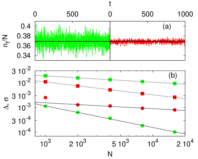
Figure 1: Panel (a). Expected values for $n_{t}/N$ in the LMG model, for $\alpha=0.5$, $E/N=-0.24$, and $N=1.6\cdot 10^{4}$. Left column (green online), state prepared following procedure (i); right column (red online), with procedure (ii). Black dotted line, analytical expected values, $\left<{\mathcal{O}}(E,\alpha)\right>$. Panel (b). Scaling as a function of the system size. Solid circles represent the distance between long-time averages and microcanonical expected values, $\Delta=\left|\overline{{\mathcal{O}}}-{\mathcal{O}}_{\text{mic}}(E,\alpha)\right|$. Solid squares, the variance of the fluctuations around the equilibrium state, $\sigma^{2}=(1/T)\int_{0}^{T}dt\,\left({\mathcal{O}}(t)-\overline{{\mathcal{O}}}\right)^{2}$. Light symbols (green online), results obtained following procedure (i); dark symbols (red online), results obtained following procedure (ii). Results are double-averaged: over the four selected observables, and over $10$ different sets of points: $\alpha=0.2$ and $E/N=-0.6$ together with $9$ different cases for $\alpha=0.5$: from $E/N=-0.26$ to $E/N=-0.22$, with steps $\Delta E/N=0.005$. Dotted and dashed lines represent fits to power-law behaviors $N^{-\gamma}$. (See main text for details).

To test if the system is properly thermalised we focus on four observables $n_{t}/N=p$, $n_{t}^{2}/N^{2}=p^{2}$, $n_{t}n_{s}/N^{2}=p(1-p)$, and $Q\cdot Q/N^{2}=4p(1-p)\cos^{2}q$. In panel (a) of Fig. 1 we show long-time dynamics of $n_{t}/N$, together with the corresponding microcanonical averages (see caption for details), for both the procedure (i) (left part), and the procedure (ii) (right part). In all the cases, $\alpha_{\text{ini}}$ depends on the target energy. For procedure (ii), $\alpha_{\text{int}}=0.25$ if $\alpha=0.2$, and $\alpha_{\text{int}}=0.53$ if $\alpha=0.5$ Supl . In panel (b), we present a quantitative test to corroborate that the system is properly thermalised. We display how the size of the fluctuations (squares) and the distance between long-time and microcanonical averages (circles) scale with the system size. Displayed data are the result of a double averaging: over $10$ different initial states $(E,\alpha)$ (see caption of Fig. 1 for details), chosen according to the findings coming from Fig. 2, and over the four selected observables. The size of the fluctuations around the equilibrium state decreases with the system size following power laws, $N^{-\gamma}$, with $\gamma=0.253(3)$ for procedure (i), and $\gamma=0.517(9)$, for procedure (ii). This means that the system remains close to the equilibrium state during the majority of the time. The distance between microcanonical and long-time averages also decreases with the system size following power laws, with exponents $\gamma=0.87(2)$ for procedure (i), and $\gamma=0.24(2)$ for procedure (ii) nota . So, we can infer that the system seems thermalised.

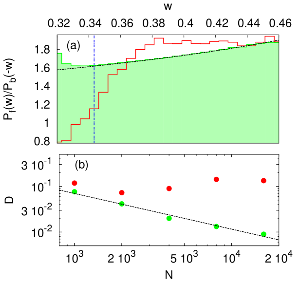
Figure 2: Panel (a). Statistics of work resulting from forward $\alpha_{i}=0.2\rightarrow\alpha_{f}=0.5$, and backwards $\alpha_{i}=0.5\rightarrow\alpha_{f}=0.2$ processes, in the LMG model with $N=1.6\cdot 10^{4}$. Filled histogram (green online), initial equilibrium states prepared following procedure (i). Empty histogram (red online), following procedure (ii). Dotted black line, results of Eq. (1). Vertical line, particular case studied in panel (a) of Fig. 4. Panel (b). Scaling of the distance, $D=(1/N)\sum_{i}\left|h(w_{i})-h_{\text{QFR}}(w_{i})\right|/h_{\text{QFR}}(w_{i})$, where $h(w_{i})$ is the height of the actual histogram at work $w_{i}$; $h_{\text{QFR}}$ the theoretical value, Eq. (1), and $N$ the number of bins. Light circles (green online), results following procedure (i). Dark circles (red online), results following procedure (ii). Dashed black line, power-law fit, $N^{-\gamma}$.

In Fig. 2 we summarize the statistics of work during non-equilibrium processes. We perform a forward process, $\alpha_{i}=0.2\rightarrow\alpha_{f}=0.5$, and the corresponding backwards one, $\alpha_{i}=0.5\rightarrow\alpha_{f}=0.2$. For the first one, we prepare two different initial states, with $E/N=-0.6$, by means of procedures (i) and (ii). For the second one, we prepare $50$ different initial states, with $25$ different energies, from $E/N=-0.26$ to $E/N=-0.14$, with steps $\Delta E/N=5\cdot 10^{-3}$ note2 , by means of procedures (i) and (ii). All the processes are performed following a TPM scheme Supl . The quotient $P_{f}(E,\alpha_{i};w)/P_{b}(E+w,\alpha_{f},-w)$ is displayed in panel (a) of Fig. 2 (see caption for details). Procedure (i) gives rise to statistics compatible with Eq. (1), but fluctuations of work coming from procedure (ii) are totally different from the expected. In panel (b) we show how the distance between numerics and Eq. (1) scales with the system size. Whereas this distance decresases following a power law for procedure (i), $N^{-\gamma}$ with $\gamma=0.78(6)$, we see no such decreasing for procedure (ii); the relative error, $D$, in the last case is quite large, around $10\%$, for system sizes between $N=10^{3}$ and $N=1.6\cdot 10^{4}$. It is worth to remark that the region in which this error is largest, $w=0.34-0.38$, is precisely the one that seemed perfectly thermalised in Fig. 1.

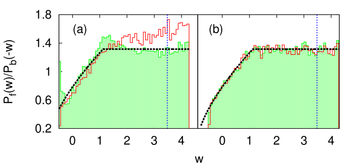
Figure 3: Statistics of work of the procedures $\alpha=1.2$ $\rightarrow$ $\alpha=2.0$ $\rightarrow$ $\alpha=0.6$ (empty histograms, red online), and $\alpha=1.2$ $\rightarrow$ $\alpha=0.0$ $\rightarrow$ $\alpha=0.6$ (full histograms, green online), in the Dicke model. Panel (a). Fock initial states. Panel (b) Microcanonical initial ensembles. The dotted black line represents the theoretical result from Eq. (1). Vertical dotted line (blue online) indicate the cases displayed on panel (b) of Fig. 4.

Different trajectories.- Here, we rely on the Dicke model Dicke:54 , experimentally realized in Baumann:10 ; dicke_exp , to test how the statistics of work depend on the trajectory, if non-equilibrium processes start from actual equilibrium states, $\overline{\rho}$. The Dicke Hamiltonian models a system of $N$ two-level atoms in a monochromatic radiation field,

$$H=\omega_{o}J_{z}+\omega a^{\dagger}a+\frac{\alpha}{\sqrt{N}}\left(J_{+}+J_{-}\right)\left(a^{\dagger}+a\right).$$ (5)

$\vec{J}$ is the pseudo-spin representation of $N$ two-level atoms, with $N=2j$ (conserved). $a^{\dagger}$ ($a$) creates (annihilates) a photon with frequency $\omega$. In all the calculations, $N=50$, $\omega=\omega_{o}=1$, and the maximum number of photons is $n_{\text{max}}=700$.

The Dicke model is known to be chaotic for large values of the coupling constant $\alpha$ and energies above the ground-state region Bastarrachea:16c ; Relano:16 ; Buijsman:17 . In the thermodynamical limit it is described by a classical Hamiltonian with two degrees of freedom,

$$H=\omega_{o}j_{z}+\frac{\omega}{2}\left(q^{2}+p^{2}\right)+2\alpha\sqrt{j}\sqrt{1-\frac{j_{z}^{2}}{j^{2}}}\cos\phi,$$ (6)

allowing to obtain the density of states, $g\left(E,\alpha\right)$, as we have done with the LMG model.

In this case, the consequences of Eq. (2) are tested by means of two different protocols, both starting from and ending at the same values of the coupling constant: (i) $\alpha=1.2$ $\rightarrow$ $\alpha=2.0$ $\rightarrow$ $\alpha=0.6$, and (ii) $\alpha=1.2$ $\rightarrow$ $\alpha=0.0$ $\rightarrow$ $\alpha=0.6$. Actual equilibrium states are obtained from initial Fock states, $\left|n,m_{j}\right>$, giving rise to an energy $E=\omega_{0}m_{j}+\omega n$; between all of them, we choose the best thermalised one, for each energy. Thermalisation is tested by means of $J_{z}$, $J_{x}^{2}$, $a^{\dagger}a$, and $\left(a^{\dagger}+a\right)^{2}$; we compare the exact long-time average with the quantum microcanonical average over a set of $51$ consecutive energy levels around the actual energy $E$ nota3 . The average relative error for the four observables and all the cases used to test Eq. (1) (see below for details) is $1.6\cdot 10^{-2}$. A measure of chaos is also performed. The average of $r_{n}=\text{min}\left(s_{n}/s_{n-1},s_{n-1}/s_{n}\right)$, where $s_{n}=E_{n-1}-E_{n}$, is obtained within a window of $200$ levels around $E/j=-0.12$, for the case with $\alpha=1.2$, $\left<r\right>=0.515(19)$. For the case with $\alpha=0.6$, $\left<r\right>=0.536(6)$ for the whole region $-0.6\leq E/j\leq 4.2$. Since $\left<r\right>=0.5307(1)$ for ergodic quantum systems, and $\left<r\right>=2\text{ln}2-1\sim 0.386$ for integrable ones Atas:13 , we can safely conlude that all our numerical experiments are done within the chaotic region Supl .

In panel (a) of Fig. 3 we summarize the statistics of work of both procedures (see caption for details). The initial energy for the forward process is $E/j=-0.12$; for the backward, we prepare $60$ different initial states, with $-0.6\leq E/j\leq 4.2$, with $\Delta E/j=0.08$. In panel (b) we show the same calculation, but starting from the microcanonical ensembles composed by $51$ consecutive levels around the target energy, the same used to test thermalisation. Results in panel (a) show that statistics of work clearly depend on the trajectory, contrary to what states the microcanonical quantum Crook’s theorem; in particular, the first one gives poor results for large values of the work. On the contrary, panel (b) clearly show that both trajectories are totally equivalent if the initial states are narrow microcanonical ensembles. For the microcanonical initial states (obtained for $w\in(0,4.3)$, to avoid data with few statistics), the average relative errors form Eq. (1) are $3.6\%$, for trajectory (i), and $3.2\%$, for trajectory (ii). The same errors are $12.3\%$ and $8.0\%$, for Fock initial states.

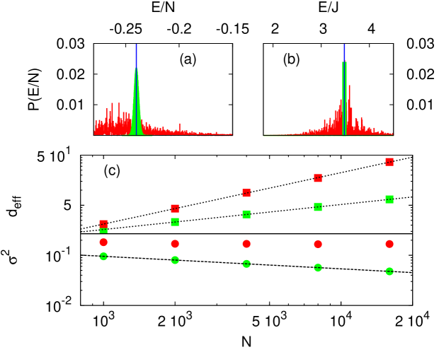
Figure 4: Panel (a). Energy distributions resulting from procedure (i), filled curve (green online), and (ii), empty curve (red online); both are obtained with the LMG model with $\alpha=0.5$, $E/N=-0.24$ and $N=1.6\cdot 10^{4}$. Dotted black line display the corresponding energies. Panel (b). Energy distribution for the Dicke model with $\alpha=0.6$ and $E/j=3.48$: empty curve (red online) correspond to initial Fock state; filled curve (green online), to microcanonical ensemble. Again, dotted black line display the corresponding energies. Panel (c). Scaling of the variance of the energy distribution, $\sigma^{2}$, as a function of the number of atoms, $N$ (solid circles); and scaling of the effective dimension of the Hilbert space, $d_{\text{eff}}$ (solid squares). Both are obtained with the LMG model. Light symbols (green online), results from procedure (i); dark symbols (red online), from procedure (ii). Dashed black line, power-law fit, $N^{-\gamma}$; dotted black line, power-law fit, $N^{\beta}$.

Discussion.- Fig. 4 provides a deeper insight on these results. Panels (a) and (b) show the energy distributions for the cases enhanced in Figs. 2 and 3 (see caption for details). Panel (a) shows the results for the LMG model. Procedure (i) gives rise to a narrow and smooth energy distribution, whereas the one corresponding to procedure (ii) is wide and erratic. Panel (b) displays the results for the Dicke model. The initial Fock state gives rise to a distribution similar to the one corresponding to procedure (ii) in panel (a), whereas the microcanonical ensemble is pretty similar to the corresponding to procedure (i). A quantitative test is performed in the LMG model, and shown in panel (c). The variance of the distribution decreases following a power law, $\sigma\sim N^{-\gamma}$, $\gamma=0.25003(3)$, if the state is prepared with procedure (i), as it is expected Schliemann:15 , but it remains approximately constant with procedure (ii). A measure of the number of populated levels, $d_{\text{eff}}=1/\sum_{n}p_{n}^{2}$, where $p_{n}$ is the probability of occupation of the level with energy $E_{n}$, is also displayed in the Figure (see caption for details). In both cases, $d_{\text{eff}}\sim N^{\beta}$, with $\beta=0.50013(3)$ for procedure (i), again as it is expected Bastarrachea:16b , and $\beta=1.027(7)$, for procedure (ii). In both cases, $d_{\text{eff}}$ grows with the number of atoms, as it is required for equilibration Gogolin:16 , but only in the case of procedure (i) $d_{\text{eff}}$ represents a negligible part of the spectrum, $d_{\text{eff}}/N\rightarrow 0$; in the case of procedure (ii) the ratio $d_{\text{eff}}/N$ is approximately the same for very different system sizes.

All these findings show that both procedure (ii) for the LMG model, and Fock initial states for the Dicke model, produce initial states too wide to fulfill the condition for the microcanonical quantum Crook’s theorem, Eq. (2), but narrow enough to seem properly thermalised. So, we conclude that

The microcanonical quantum Crook’s theorem consititues a more stringent test of thermalisation than the expected values of observables in equilibrium.

Hence, experiments involving quantum fluctuation theorems Chiara:15 ; An:15 can disclose non-proper thermalisation.

- (1) I. Bloch, J. Dalibard, and W. Zwerger, Rev. Mod. Phys. 80, 885 (2008).
- (2) T. Langen, R. Geiger, and J. Schmiedmayer, Ann. Rev. Cond. Mat. Phys. 6, 201 (2015).
- (3) J. Gemmer, M. Michel, and G. Mahler, Quantum Thermodynamics, Lecture Notes in Physics 784, Berlin Springer (2009).
- (4) M. Greiner, O. Mandel, T. W. Hänsch, and I. Bloch, Nature 419, 51 (2002).
- (5) C. Gross, T. Zibold, E. Nicklas, J. Esteve, and M. K. Oberthaler, Nature 464, 1165 (2010); T. Zibold, E. Nicklas, C. Gross, and M. K. Oberthaler, Phys. Rev. Lett. 105, 204101 (2010).
- (6) M. Albiez, R. Gati, J. Fölling, S. Hunsmann, M. Cristiani, and M. K. Oberthaler, Phys. Rev. Lett. 95, 010402 (2005).
- (7) A. Trenkwalder, G. Spagnolli, G. Semeghini, S. Coop, M. Landini, P. Castiho, L. Pezzé, G. Modugno, M. Inguscio, A. Smerzi, and M. Fattori, Nat. Phys. 12, 826 (2015).
- (8) M. J. Martin, M. Bishof, M. D. Swallows, X. Zhang, C. Benko, J. von-Stecher, A. V. Gorshkov, A. M. Rey, and J. Ye, Science 341, 632 (2013).
- (9) C. S. Gerving, T. M. Hoang, M. Anquez, C. D. Hamley, and M. S. Chapman, Nat. Comm. 3, 1169 (2012).
- (10) S. Will, T. Best, U. Schneider, L. Hacermüller, D.-S. Lühmann, and I. Bloch, Nature 465, 197 (2010).
- (11) K. Baumann, C. Guerlin, F. Brennecke, and T. Esslinger, Nature 464, 1301 (2010); K. Baumann, R. Mottl, F. Brennecke, and T. Esslinger, Phys. Rev. Lett. 107, 140402 (2011).
- (12) M. A. Alcalde, M. Bucher, C. Emary, and T. Brandes, Phys. Rev. E 86, 012101 (2012).
- (13) M. A. Bastarrachea-Magnani, S. Lerma-Hernńdez, and J. G. Hirsch, J. Stat. Mech. (2016) 093105.
- (14) P. Pérez-Fernández and A. Relaño, Phys. Rev. E 96, 012121 (2017).
- (15) R. H. Dicke, Phys. Rev. 93, 99 (1954).
- (16) H. J. Lipkin, N. Meshkov, and A. J. Glick, Nucl. Phys. 62, 188 (1965).
- (17) M. A. Cazalilla and M. Rigol, New. J. Phys. 12, 55006 (2010).
- (18) A. Polkovnikov, K. Sengupta, A. Silva, and M. Vengalattore, Rev. Mod. Phys. 83, 863 (2011).
- (19) J. Eisert, M. Friesdorf, and C. Gogolin, Nat. Phys. 11, 124 (2015).
- (20) C. Gogolin and J. Eisert, Rep. Prog. Phys. 79, 056001 (2016).
- (21) J. Neumann, Z. Phys. 57, 30 (1929); J. Neumann, Eur. Phys. J. H 35, 201 (2010); S. Goldstein, J. L. Lebowitz, C. Mastrodonato, R. Tumulka, and N. Zanghi, Proc. R. Soc. A 466, 3203 (2010).
- (22) A. J. Short, New. J. Phys. 13, 053009 (2011); A. J. Short and T. C. Farrelly, New. J. Phys. 14, 013063 (2012); P. Reimann and M. Kastner, New. J. Phys. 14, 043020 (2012).
- (23) M. Srednicki, J. Phys. A 29, 175 (1996).
- (24) R. V. Jensen and R. Shankar, Phys. Rev. Lett. 54, 1879 (1985); J. M. Deutsch, Phys. Rev. A 43, 2046 (1991); M. Srednicki, Phys. Rev. E 50, 888 (1994); H. Tasaki, Phys. Rev. Lett. 80, 1373 (1998); M. Rigol, V. Dunjko, and M. Olshanii, Nature 452, 854 (2008).
- (25) C. Jarzynski, Phys. Rev. Lett. 78, 2690 (1997).
- (26) G. E. Crooks, Phys. Rev. E 60, 2721 (1999).
- (27) P. Talkner, E. Lutz, and P. Hänggi, Phys. Rev. E 75, 050102 (2007).
- (28) M. Campisi, P. Hänggi, and P. Talkner, Rev. Mod. Phys. 83, 1653 (2011).
- (29) L. D’Alessio, Y. Kafri, A. Polkovnikov, and M. Rigol, Adv. Phys. 65, 239 (2016).
- (30) P. Talkner, P. Hänggi, and M. Morillo, Phys. Rev. E 77, 051131 (2008).
- (31) There is some controversy about the definition of work and the way to meassure it, in a non-equilibrium protocol (see, for example, Perarnau:17 ). Here, we assume that a two-projective measurement (TPM) scheme is used. All our calculations are fully compatible with this scheme.
- (32) M. Perarnau-Llobet, E. Bäumer, K. V. Hovhannisyan, M. Huber, and A. Acin, Phys. Rev. Lett. 118, 070601 (2017); M. Lostaglio, Phys. Rev. Lett. 120, 040602 (2018).
- (33) More details are given in the Supplementary Material to this Letter.
- (34) We find power laws instead of exponential decays due to the collective nature of the system, making the dimension of the Hilbert space grow linearly (instead of exponentially) with the number of atoms. Anyhow, both distances are small even at moderate system sizes, .
- (35) R. G. Unanyan and M. Fleischhauer, Phys. Rev. Lett. 90, 133601 (2003).
- (36) A. Micheli, D. Jaksch, J. I. Cirac, and P. Zoller, Phys. Rev. A 67, 013607 (2003).
- (37) S. Morrison and A. S. Parkins, Phys. Rev. Lett. 100, 040403 (2008); Phys. Rev. A 77, 043810 (2008).
- (38) J. Larson, EPL 90, 54001 (2010).
- (39) J. Vidal, J. M. Arias, J. Dukelsky, and J. E. García-Ramos, Phys. Rev. C 73, 054305 (2006).
- (40) M. A. Caprio, P. Cejnar, and F. Iachello, Ann. Phys. (N.Y.) 323, 1106 (2008); A. Relaño, J. M. Arias, J. Dukelsky, J. E. García-Ramos, and P. Pérez-Fernández, Phys. Rev. A 78, 060102(R) (2008); P. Pérez-Fernández, A. Relaño, J. M. Arias, J. Dukelsky, and J. E. García-Ramos, Phys. Rev. A 80, 032111 (2009).
- (41) Note that Eq. (1) requires that the backward process starts at the energy resulting from the forward. If initial energy is , and the measured work, , the backward process must start from a thermalised state with energy to properly test Eq. (1). Hence, we require just an initial state with energy for the forward process, but a number of initial states with energies , covering all the measured values for the work, .
- (42) M. P. Baden, K. J. Arnold, A. L. Grimsmo, S. Parkins, and M. D Barrett, Phys. Rev. Lett. 113, 020408 (2014), ibid 118, 199901 (2017); C. Hamner, C. Qu, Y. Zhang, J. Chang, M. Gong, C. Zhang, and P. Engels, Nat. Comm. 5, 4023 (2014).
- (43) M. A. Bastarrachea-Magnani, S. Lerma-Hernández, and J. G. Hirsch, Phys. Rev. A 89, 032101 (2014).
- (44) A. Relaño, M. A. Bastarrachea-Magnani, and S. Lerma-Hernández, EPL 116, 050005 (2016); M. A. Bastarrachea-Magnani, A. Relaño, S. Lerma-Hernández, B. López del Carpio, J. Chávez-Carlos, and J. Hirsch, J. Phys. A 50, 144002 (2017).
- (45) W. Buijsman, V. Gritsev, and R. Sprik, Phys. Rev. Lett. 118, 080601 (2017).
- (46) In this case, we do not rely on a classical microcanonical average, as we have done with the LMG model, because of the finite-size effects related to the small number of atoms, , accesible to exact diagonalization.
- (47) Y. Y. Atas, E. Bogomolny, O. Giraud, and G. Roux, Phys. Rev. Lett. 110, 084101 (2013).
- (48) J. Schliemann, Phys. Rev. A 92, 022108 (2015).
- (49) M. A. Bastarrachea-Magnani, B. López-del-Carpio, J. Chávez-Carlos, S. Lerma-Hernández, and J. G. Hirsch, Phys. Rev. E 93, 022215 (2016).
- (50) G. De. Chiara, A. J. Roncaglia, and J. P. Paz, New. J. Phys. 15, 035004 (2015).
- (51) S. An, J.-N. Zhang, M. Um, P. Lv, Y. Lu, J. Zhang, Z.-Q. Yin, H. Y. Quan, and K. Kim, Nat. Phys. 11, 193 (2015).