Quantum fluctuations of the compact phase space cosmology

Abstract

In the recent article Phys. Rev. D 100, no. 4, 043533 (2019) a compact phase space generalization of the flat de Sitter cosmology has been proposed. The main advantages of the compactification is that physical quantities are bounded, and the quantum theory is characterized by finite dimensional Hilbert space. Furthermore, by considering the $\mathbb{S}^{2}$ phase space, quantum description is constructed with the use $SU(2)$ representation theory. The purpose of this article is to apply effective methods to extract semi-classical regime of the quantum dynamics. The analysis is performed both without prior solving of the quantum constraint and by extracting physical Hamiltonian of the model. At the effective level, the results of the two procedures are shown to be equivalent. We find a nontrivial behavior of the fluctuations around the recollapse of the universe, which is distinct from what is found after quantization with the standard flat phase space. The behavior is reflected at the level of the modified Friedmann equation with quantum back-reaction effects, which is derived. Finally, an unexpected relation between the quantum fluctuations of the cosmological sector and the holographic Bousso bound is shown.

I Introduction

Twenty-three years after the surprising proposition by Einstein that spacetime might not be linear, Born suggested in 1938 that the conjugated momentum space might be curved as well Born49 . From then, many models with non-linear momentum space have been developed. As showed in the geometrical approach Ashtekar:1997ud , many generalizations of quantum mechanics may arise at a more fundamental level by considering a non-linear phase space. In $q$-deformation theories or in non-commutative geometry, the non-linearity of momentum space is presented as a way to introduce non-commutativity of spacetime (Snyder:1946qz, ; Majid:1999tc, ; Connes:1994yd, ). On the other hand, such a geometry of momentum space may lead to a relative notion of locality (AmelinoCamelia:2011bm, ; AmelinoCamelia:2011pe, ). Beyond this non-linear property, a particularly interesting case is that of a compact momentum space. In Loop Quantum Gravity (LQG) Ashtekar:2004eh ; Rovelli:1997yv and Loop Quantum Cosmology (LQC) Bojowald:2008zzb , compactification of the momentum space is introduced as a way to imply discreteness of length, area and volume operators, which de facto resolves the Big Bang singularity Bojowald:2001xe . This feature is the exact analogue of the discrete spectrum of momentum operator in usual quantum mechanics, when considering a compact position operator Rovelli:2014ssa .

A natural and relevant way of extending those works could, therefore, be to consider both canonical variables to be non-linear, and eventually compact. Such studies have for example been conducted in the context of (3+1)-dimensional lattice Yang-Mills theory (Riello:2017iti, ; Dittrich:2017nmq, ) and of LQG Haggard:2015ima . The recently introduced Non-linear Field Space Theory (NFST) program Mielczarek:2016rax aims to generalize and unify the phase-space compactification process to all field theories (Bilski:2017gic, ; Mielczarek:2017ny, ). In NFST, the phase space is compact and canonical variables are, therefore, bounded. This naturally satisfies Born’s principle of finiteness Born:1934fy and implies that, at the quantum level, the Hilbert space has finite dimension. In addition, a compact phase space opens a way to describe fields with the use of spin variables Mielczarek:2016xql .

One goal is to apply the NFST formalism to the gravitational field. This is an interesting application because it may allow to avoid infrared and ultraviolet singularities. For example, in Guimarey:2019lmn it has been shown that the compactification of the phase space of the gravitational field at the level of a minisuperspace leads to a phase of recollapse, rather than a phase of infinite expansion, even in a universe dominated by dark energy (cosmological constant). Moreover, such a generalization is also motivated by loop quantum cosmology, where the phase space is already compactified in the momentum direction, leading to a cylindrical phase space. This momentum compactification implies to a resolution of the big bang singularity. However, in sufficiently flat universes it is expected that the universe will enter a phase of eternal expansion, which amounts to an infrared divergence. The compactification of the remainder of the phase space, cures this divergence, leading to a universe with many cycles of expansion and collapse.

The classical properties of a minisuperspace model with a compact phase space can be obtained in a straightforward manner, and in some situations exact solutions can be derived. After its quantization, it is possible to solve the model exactly in the case where the spin is small or when $s\sim\hbar$. Solutions for arbitrary spin $s$ are shown to exist but are, from a mathematical point of view, difficult to extract. However, in order to investigate the semiclassical limit, we need to solve the case where the spin is very large compared to $\hbar$, which is the goal of this paper.

Worth emphasizing is that the minisuperspace semiclassical sector, described in NFST cosmology by a state in $2s+1$ dimensional Hilbert space of a spin $s$, can be interpreted as a maximal spin subspace of a higher dimensional product space of fundamental representations of SU(2) - spin-1/2. This paves a way to both extract quantum cosmological sector from dynamics of elementary (inhomogeneous) spin-1/2 degrees of freedom and to consider analog cosmological models employing condensed matter systems and quantum information processing technologies.

The objective of this article is to implement a semiclassical analysis of the model presented in Guimarey:2019lmn . The Poisson bracket of this model is the bracket of $\mathrm{su}(2)$ algebra. Since this bracket is non-canonical the model is most easily quantized by the canonical quantization. However, the model is also constrained, owing to the fact that it is derived from general relativity (GR). The most systematic way of dealing with such a system at the effective level is by way of the canonical effective methods Bojowald:2009 . Therefore, we are formulating the dynamics of our system in terms of expectation values and their fluctuations, rather than in terms of wave functions. In the semiclassical limit, where higher order moments can be ignored this leads to a much more manageable system of ordinary differential equations rather than partial differential equations.

In order to explain the idea of NFST cosmology, we first present a model of LQC in Sec. II, which can be considered as a limiting case of compact phase space cosmology. Instead of following the usual construction of LQC, we adopt the point of view of momentum polymerization which focuses on the geometry of the phase space. Generalizing such a construction, we present in Sec. III the de Sitter model with compact phase space that has been derived and analyzed in details in Guimarey:2019lmn . The core of this article is contained in Sec. IV, where the semiclassical limit of our model is derived by means of canonical effective methods. Finally, in Sec. V we give physical analysis concerning such issues as: the number of elementary (inhomogeneous) degrees of freedom required to construct the semiclassical cosmological state, estimation of the magnitude of the quantum fluctuations and the fate of the holographic Bousso bound are discussed.

II de Sitter model in Loop Quantum Cosmology

II.1 Classical Kinematics

Let us first consider the case with the flat phase space. Since we are studying the canonical evolution of the Universe, we introduce a canonical physical co-volume $q$, depending on the scale factor $a$ and a fiducial volume of an elementary cell $V_{0}$, such that $|q|:=V_{0}a^{3}$. We introduce the corresponding canonical momentum variable $p$. In physical terms, this canonical momentum is proportional to the Hubble parameter. The phase space $(p,q)$ is therefore a symplectic manifold equipped with a closed 2-form $\omega$ which can be expressed in a Darboux form:

$$\omega=dp\wedge dq.$$ (1)

The inversion of the symplectic form (1) gives the usual Poisson bracket of the considered algebra:

$$\{f,g\}:=(\omega^{-1})^{ij}\partial_{i}f\partial_{j}g=\frac{\partial f}{\partial q}\frac{\partial g}{\partial p}-\frac{\partial f}{\partial p}\frac{\partial g}{\partial q},$$ (2)

for two arbitrary functions $f$ and $g$ defined on the phase space.

II.2 Classical Dynamics

In order to study the dynamics of our cosmological system, we now have to identify a suitable Hamiltonian $\mathcal{H}=NC$, such that any variable $f$ would evolve as

$$\dot{f}=\{f,\mathcal{H}\}$$ (3)

where $\dot{f}:=df/dt$ denotes the usual derivative along some time parameter $t$. In classical GR, the de Sitter Hamiltonian constraint for non-vanishing cosmological constant $\Lambda$ is

$$C_{\text{GR}}=q\left(-\frac{3}{4}\kappa p^{2}+\frac{\Lambda}{\kappa}\right),$$ (4)

where $q,p\in\mathbb{R}$, $\kappa:=8\pi G$ and $N$ is the lapse function.

Solving the dynamics of our system is equivalent to solving and integrating the constraint equation $\partial\mathcal{H}/\partial N=0$. This constraint is characteristic of any time-reparametrization invariant theory, such as GR. If we include some ordinary matter content, solving the constraint for the classical Hamiltonian (4) leads to the well-known Big Bang singularity with cosmological constant $\Lambda$.

A common way for resolving the UV divergence (i.e. the Big Bang singularity) is that of loop quantum cosmology, which consists of the so-called momentum polymerization $p\in(-\infty,+\infty)\rightarrow\lambda p\in[-\pi,+\pi]$, where $\lambda$ is a physical length arising from discretization of lengths in loop quantum gravity Agullo:2013dla , and we can generalize the Hamiltonian to be

$$C_{\text{LQC}}=q\left(-\frac{3}{4}\kappa\frac{\sin^{2}(\lambda p)}{\lambda^{2}}+\frac{\Lambda}{\kappa}\right).$$ (5)

Notice that the polymerization of momentum $p\in[-\pi/\lambda,\pi/\lambda]$ usually performed in LQC doesn’t change the symplectic structure. This is because one can always choose a local coordinate system on their symplectic manifolds to bring the symplectic structure into canonical form. In this example we have chosen to use a coordinate system with a canonical symplectic structure. However, after polymerization of both the generalized coordinate $q$ and momentum $p$ we will obtain a phase space which is equivalent to the phase space of spin, and the quantization of such a system is most easily done with a non-canonical Poisson structure. Therefore, in section (III.1) we will use a specific non-canonical bracket because it is more amenable to quantization.

As a way to characterize the rate of expansion of the Universe, it is convenient to introduce the Hubble factor $H:=\frac{\dot{a}}{a}=\frac{1}{3}\frac{\dot{q}}{q}$. By using (3), we can calculate the Hubble parameter in terms of the momentum. We can then insert this result into the Hamiltonian constraint $\partial\mathcal{H}_{\text{LQC}}/\partial N=0$, and derive the effective Friedmann equation for de Sitter universe in LQC Ashtekar:2006wn ; Mielczarek:2008zv ; Mielczarek:2010rq ,

$$H^{2}=\frac{N^{2}\kappa}{3}\frac{\Lambda}{\kappa}\left(1-\frac{4\lambda^{2}}{3}\frac{\Lambda}{\kappa^{2}}\right)=\frac{N^{2}\kappa}{3}\rho_{\Lambda}\left(1-\frac{\rho_{\Lambda}}{\rho_{c}}\right),$$ (6)

where we defined the cosmological constant energy density $\rho_{\Lambda}:=\Lambda/\kappa$ and the critical energy density $\rho_{c}:=3\kappa/4\lambda^{2}$. We notice that this model is equivalent to a classical de Sitter model with a renormalized cosmological constant. When taking ordinary matter into account, this effective Friedmann equation turns out to replace the Big Bang singularity by a Big Bounce instead, already at the semiclassical level Ashtekar:2006wn ; Dzierzak:2009ip .

III de Sitter model in Nonlinear Phase Space Cosmology

III.1 Kinematics

The NFST aims to generalize the fundamental field theories used in physics to the case of a compact phase space (Mielczarek:2016rax, ; Mielczarek:2017ny, ). The phase space $(q,p)$ is compactified into an ellipsoid, which is conveniently parametrized by spin vector $\vec{S}=(S_{x},S_{y},S_{z})$, with components Mielczarek:2016xql :

$$\left\{\begin{array}[]{r c l}S_{x}&=&S\cos\left(\frac{p}{R_{1}}\right)\cos\left(\frac{q}{R_{2}}\right)\\ S_{y}&=&S\sin\left(\frac{p}{R_{1}}\right)\cos\left(\frac{q}{R_{2}}\right)\\ S_{z}&=&-S\sin\left(\frac{q}{R_{2}}\right)\end{array}\right.$$ (7)

with the angles $p/R_{1}\in[-\pi,\pi]$ and $q/R_{2}\in[-\pi/2,\pi/2]$. $S=\sqrt{\vec{S}\cdot\vec{S}}=R_{1}R_{2}$ and $R_{1}$, $R_{2}$ are the two axes of the ellipsoid phase space. However, we can always make a canonical transformation which sets $R_{1}=R_{2}=\sqrt{S}$. Furthermore, it is convenient to keep these as two separate parameters, because it will allow us to study various limiting cases. For example, the limit $R_{2}\rightarrow\infty$ corresponds to the phase space of LQC. As shown in Guimarey:2019lmn , the physical length $\lambda$ can be directly related to the radius of compactified momentum $\lambda:=1/R_{1}$, and the $R_{1,2}\rightarrow\infty$ limit is, therefore, equivalent to the classical affine phase space.

When considering such a spherical phase space, the symplectic 2-form should be replaced by

$$\omega=\cos{\left(\frac{q}{R_{2}}\right)}dp\wedge dq,$$ (8)

and the Poisson bracket therefore reads

$$\{f,g\}:=\frac{1}{\cos{\left(q/R_{2}\right)}}\left(\frac{\partial f}{\partial q}\frac{\partial g}{\partial p}-\frac{\partial f}{\partial p}\frac{\partial g}{\partial q}\right).$$ (9)

We, therefore, recover the standard kinematics in the limit when the phase space curvature goes to zero.

III.2 Dynamics

The compact phase space approach allows us to express the dynamics in terms of the spin variables (7). A relevant Hamiltonian constraint for describing the de Sitter model in the context of spherical phase space is the following one Guimarey:2019lmn :

$$H_{S}=NC_{S}=N\frac{S_{z}}{R_{1}}\left[\frac{3}{4}\kappa\frac{S_{y}^{2}}{R_{2}^{2}}-\frac{\Lambda}{\kappa}\right],$$ (10)

satisfying the following conditions:

$$\left\{\begin{array}[]{l c l}\lim_{R_{2}\rightarrow\infty}C_{S}&=&C_{\text{LQC}}\\ \lim_{R_{1,2}\rightarrow\infty}C_{S}&=&C_{\text{GR}}\end{array}\right..$$ (11)

For later convenience, we define the following constants:

$$\beta:=\frac{3}{2}\frac{\kappa}{R_{1}R_{2}^{2}},\quad\delta:=\frac{\rho_{\Lambda}}{\rho_{c}}=\frac{4\Lambda}{3\kappa^{2}R_{1}^{2}},$$ (12)

and fix the time gauge to $N=\frac{2}{\beta}$, such that constraint (10) takes the convenient form:

$$C_{S}=S_{z}\left[S_{y}^{2}-\delta S^{2}\right].$$ (13)

Employing the Hamilton equation for $q$, we deduce the Hubble factor at the kinematical level:

$$H=-\frac{1}{2}\frac{\kappa}{S^{2}q}\frac{S_{x}S_{y}S_{z}}{\cos{(q/R_{2})}}.$$ (14)

Imposing then the constraint $\partial H_{S}/\partial N=0$, the Friedmann equation can be derived Guimarey:2019lmn :

$$H^{2}=N^{2}\frac{\Lambda}{3}\left(\frac{\sin(q/R_{2})}{q/R_{2}}\right)^{2}\left[\frac{\cos^{2}\left(q/R_{2}\right)-\delta}{\cos^{2}(q/R_{2})}\right].$$ (15)

This generalized Friedmann equation ensures that the volume $q$ is bounded from above, implying a phase of recollapse for the Universe. In addition, it can be shown that in the limit $R_{2}\rightarrow\infty$, we recover the Friedmann equations of LQC (6). We therefore suspect that, adding another matter field, the generalized Friedmann equation of NFST could lead to an oscillating Universe.

From the Hamiltonian (13) and the Poisson structure (9) we can determine the evolution of the spin variable:

$$\left\{\begin{array}[]{r c l}\dot{S_{x}}&=&2S_{y}S_{z}^{2}+\left(\delta S^{2}-S_{y}^{2}\right)S_{y},\\ \dot{S_{y}}&=&S_{x}\left(S_{y}^{2}-\delta S^{2}\right),\\ \dot{S_{z}}&=&-2S_{x}S_{y}S_{z}.\end{array}\right.$$ (16)

We can therefore fully describe the dynamics of our system by restricting the spin variable to the surface of constraint. This requires to solve the Hamiltonian constraint, here equivalent to $S_{y}=\pm\sqrt{\delta}S$, which then leads to the dynamical equations:

$$\left\{\begin{array}[]{r c l}\dot{S}_{x}&\approx&N\beta S_{y}S_{z}^{2},\\ \dot{S}_{y}&\approx&0,\\ \dot{S}_{z}&\approx&-N\beta S_{x}S_{y}S_{z}.\end{array}\right.$$ (17)

where $N\beta=2$, but we here made the choice to write $N$ explicitly.

III.3 Physical Hamiltonian

We would now like to determine a physical Hamiltonian of our system $p_{\phi}$, that directly generates the dynamics of the spin variable on the surface of constraint (17). This physical Hamiltonian is by definition the generator of a physical time, that we will d escribe as a scalar field $\phi$. It thus satisfies the new Poisson bracket relation $\phi^{\prime}:=\{\phi,p_{\phi}\}_{\phi,p_{\phi}}=1$, where the prime denotes derivative with respect to the physical time $(^{\prime}:=d/d\phi)$. By definition, under this time reparametrization $t\rightarrow\phi$, the lapse function becomes $N\rightarrow\tilde{N}=N(d\phi/dt)^{-1}$.

The equations of motion (17) are then given by

$$\dot{S_{i}}=\frac{d\phi}{dt}S_{i}^{\prime}=\frac{d\phi}{dt}\{S_{i},p_{\phi}\}_{\phi,p_{\phi}}.$$ (18)

We need to choose the specific physical time such that the resulting system of differential equations is actually a Hamiltonian system. To accomplish this we notice that $\dot{S}_{y}\approx 0$ implies the physical Hamiltonian can only depend on $S_{y}$. From the Leibniz rule then, it follows that the equations of motion with respect to the physical time should have the following behavior $S^{\prime}_{x}\propto S_{z}$ and $S^{\prime}_{z}\propto S_{x}$. To accomplish this we define our physical time implicitly in the following way:

$$\tilde{N}=N\left(\frac{d\phi}{dt}\right)^{-1}=N\left(S_{z}\right)^{-1}.$$ (19)

The equations of motion (17) are then equivalent to:

$$\left\{\begin{array}[]{r c l}S_{x}^{\prime}&=&\tilde{N}\beta S_{y}S_{z}^{2}=2S_{y}S_{z},\\ S_{y}^{\prime}&=&0,\\ S_{z}^{\prime}&=&-\tilde{N}\beta S_{x}S_{y}S_{z}=-2S_{x}S_{y}.\end{array}\right.$$ (20)

This choice of physical time therefore makes the equations of motion much easier to deal with, furthermore this system of equations is now a Hamiltonian system, as required. In fact, not every choice of time parametrization will lead to equations of motion on the constraint surface that are Hamiltonian. The choice we make here does, but we also make this choice because it leads to a physical Hamiltonian that is quadratic and therefore amenable to quantization. However, one should notice that when the Universe will collapse, $\tilde{N}$ goes to infinity as the physical volume goes to 0 (i.e. $S_{z}\rightarrow 0$). In consequence, it will be more convenient to go back to the parameter time $t$ when analyzing the dynamics close to a singularity. From equations (20), one can easily deduce the corresponding physical Hamiltonian $p_{\phi}=S_{y}^{2}$.

Time in General Relativity is difficult to define, as it is a relational quantity Rovelli:2004tv ; Bojowald:2010qpa . The way to notice the flow of time is by describing how some objects evolve in relation with a distinguished degree of freedom that can play the role of time. In our simplistic model, the only matter present in the Universe is the cosmological constant. We’ve seen that the equations of motion (17) satisfied the constraint $S_{y}^{2}=\delta S^{2}$. However, our derivation of a physical Hamiltonian therefore implies that $p_{\phi}=S_{y}^{2}=\delta S^{2}$. Choosing a time parametrization that makes our system Hamiltonian on the constraint surface therefore leads us to the interpretation that the cosmological constant is the momentum of a scalar field. This implied scalar field can then play the role of time.

III.4 Quantization

Since our model is expressed in terms of spin variables we can quantize it in the usual way: $S_{i}\rightarrow\hat{S}_{i}$. However, since we are working with a constrained system there are two ways we can proceed. We can quantize before or after gauge fixing. It turns out that these two approaches agree to first order quantum corrections. Quantizing after gauge fixing is most straightforward way to proceed. The deparametrized Hamiltonian corresponding to (13) is: $p_{\phi}=S_{y}^{2}$, which has the simple quantization:

$$\hat{p}_{\phi}=\hat{S}_{y}^{2}.$$ (21)

This system is actually solvable exactly. If we work in a basis that diagonalizes $S_{y}$. However, since we are only interested in semiclassical states, this analysis is not necessary for us.

We can instead choose to quantize the constraint (13) before gauge fixing, we obtain the following quantum constraint:

$$\hat{C}_{S}=\left(\hat{S}_{z}\hat{S}_{y}^{2}\right)_{\text{Weyl}}-\left(\hat{S}_{z}\hat{p}_{\phi}\right)_{\text{Weyl}},$$ (22)

where we made the choice to use Weyl ordering of all the operators, we have also made the choice to not include factorial powers of the $\hat{S}_{i}$ in the ordering choice. Moreover, $\left(...\right)_{\text{Weyl}}$ refers to the usual Weyl ordering, e.g.:

$$\left(\hat{S}_{z}\hat{S}_{y}^{2}\right)_{\text{Weyl}}:=\frac{1}{3}\left(\hat{S}_{z}\hat{S}_{y}\hat{S}_{y}+\hat{S}_{y}\hat{S}_{z}\hat{S}_{y}+\hat{S}_{y}\hat{S}_{y}\hat{S}_{z}\right).$$ (23)

We are not aware of a method to solve this constraint exactly for arbitrary choice of $s$. However, after fixing $s$ to a certain value, solving the constraint is equivalent to finding its null space, which can always be done, at least numerically for finite systems. As an example, exact solutions have been derived for low spin value $s=2$ in Guimarey:2019lmn .

IV Semiclassical limit of de Sitter in NFST

Solving the quantum constraint in full generality is a hard problem. Additionally, solving the deparametrized constraint is possible, however, we don’t have a satisfactory way of selecting suitable initial conditions. Despite these difficulties, we are most interested in the behavior of our system in the semiclassical regime which can be accessed with the canonical effective methods. This is an interesting approach because it will allow us to see how the quantum fluctuations behave in the presence of a spherical phase space without having to solve the quantum dynamics exactly.

IV.1 Semiclassical Mechanics

After we have identified our classical phase space as the phase space of spin, our Poisson bracket takes the form: $\left\{S_{i},S_{j}\right\}=\varepsilon_{ijk}S_{k}$. The quantization of this bracket can be found with the usual canonical quantization. However, we aim to perform a semiclassical analysis of this system, which will involve studying the backreaction of the moments onto the expectation values of the spin. We therefore need to understand the kinematics of the moments of the state. At the semiclassical level, the required Poisson brackets can be defined in a straightforward way Baytas:2017eq33 :

$$\left\{\langle\hat{A}\rangle,\langle\hat{B}\rangle\right\}=\frac{1}{i\hbar}\left\langle\left[\hat{A},\hat{B}\right]\right\rangle.$$ (24)

Where this bracket is augmented with the Leibniz rule in order to satisfy all the properties of a Poisson bracket. Truncating our results at the leading semiclassical correction yields the following algebra of moments:

$$\begin{split}\left\{S_{i},S_{j}\right\}&=\varepsilon_{ijk}S_{k},\\ \left\{\Delta\left(S_{a}S_{b}\right),S_{c}\right\}&=\varepsilon_{acd}\Delta(S_{d}S_{b})+\varepsilon_{bcd}\Delta(S_{d}S_{a}),\\ \left\{\Delta(S_{a}S_{b}),\Delta(S_{c}S_{d})\right\}&=\varepsilon_{ace}S_{e}\Delta(S_{b}S_{d})+\varepsilon_{bce}S_{e}\Delta(S_{a}S_{d})\\ &+\left(c\leftrightarrow d\right)+O(\hbar^{3/2}).\end{split}$$ (25)

Given a Hamiltonian, we can use this Poisson algebra to generate equations of motion on the semiclassical phase space. Moreover, this Poisson bracket is triply degenerate, admitting three Casimir functions. One of them takes the simple form: $\mathcal{C}_{1}=\langle\hat{S}^{2}\rangle=\vec{S}^{2}+\Delta(\vec{S}^{2})$. Due to this degeneracy, the expectation value of $\vec{S}^{2}$ is a constant of the motion, which is not surprising because this operator commutes with all Hamiltonians constructed from the spin operators. The second Casimir takes the form: $\mathcal{C}_{2}=2S_{i}\Delta(S_{i}S_{j})S_{j}+\Delta(S_{i}S_{i})^{2}-\Delta(S_{i}S_{j})\Delta(S_{j}S_{i})$. The last and most interesting Casimir takes the form $\mathcal{C}_{3}=\det\left[\Delta(S_{i}S_{j})\right]$. This implies that the volume of the wave packet in the spin space is conserved over time. This also gives us a crude measure of semiclassicality. As in the flat case a measure of semiclassicality is area of the wave packet in phase space. Here we can use the volume of the wave packet, which happens to be a constant of the motion. Moreover, even at the level of kinematics we already have a divergence from the classical theory where the evolution is constrained to a sphere of radius $S$. Due to the quantum corrections this sphere actually becomes fuzzy and the classical spin is not conserved.

Given a Poisson bracket on the semiclassical phase space, we still need a Hamiltonian to generate dynamics. For consistency with the ordinary Schrödinger flow on the Hilbert space, the Hamiltonian on the semiclassical phase space takes the simple form $H_{Q}=\langle\hat{H}\rangle$, this expectation value can be expressed as a sum of central moments of our quantum state, which can then be truncated at the leading semiclassical order. Furthermore, this Hamiltonian is defined uniquely up to terms which depend only the Casimir function of the Poisson algebra. From here the semiclassical dynamics can be generated in the usual way: $\dot{K}=\left\{K,H_{Q}\right\}$, for some phase space function $K$.

IV.2 Effective constraints

In fact, setting the expectation value of (22) to zero is not the only constraint we need to implement at the effective level. For leading order quantum corrections, we also need to implement to following effective constraints:

$$\begin{split}C^{q}_{s}&=\langle\hat{C}_{s}\rangle=S_{z}(S_{y}^{2}-p_{\phi})+S_{z}\Delta(S_{y}^{2})\\ &+2S_{y}\Delta(S_{z}S_{y})-\Delta(S_{z}p_{\phi}),\\ C_{S_{i}}&=\langle\hat{C}_{s}\hat{\delta}S_{i}\rangle_{W}=2S_{y}S_{z}\Delta(S_{y}S_{i})-S_{z}\Delta(p_{\phi}S_{i}),\\ C_{p\phi}&=\langle\hat{C}_{s}\hat{\delta}p_{\phi}\rangle_{W}=2S_{z}S_{y}\Delta(S_{y}p_{\phi})-S_{z}\Delta(p_{\phi}^{2}),\\ C_{\phi}&=\langle\hat{C}_{s}\hat{\delta}\phi\rangle_{W}=2S_{z}S_{y}\Delta(S_{y}\phi)-S_{z}\Delta(p_{\phi}\phi).\end{split}$$ (26)

A direct calculation shows that these constraints are preserved under evolution with respect to the coordinate time, that is, $\left\{C_{s}^{q},C_{i}\right\}=0$. Moments involving $\phi$ can be chosen by a gauge choice and moments involving $p_{\phi}$ are selected by the constraints. In particular we have

$$\Delta(p_{\phi}S_{z})=2S_{y}\Delta(S_{y}S_{z}).$$ (27)

Inserting this into the quantum constraint and solving for $p_{\phi}$, we find the following deparametrized Hamiltonian

$$p_{\phi}=S_{y}^{2}+\Delta(S_{y}^{2})+O(\hbar^{2}).$$ (28)

This is a quadratic Hamiltonian now, and furthermore, it is what we would expect from the quantization of deparametrized Hamiltonian (21). We also notice that both terms in this Hamiltonian are conserved separately. This can be seen by directly calculating the equations of motion with respect to the internal time:

$$\begin{split}S^{\prime}_{y}&=0,\\ \Delta(S_{y}^{2})^{\prime}&=0.\end{split}$$ (29)

The other equations of motion can be derived in the usual way: $K^{\prime}=\left\{K,p_{\phi}\right\}$. Using the Poisson bracket (25) and the semiclassical Hamiltonian we find the following explicit equations of motion:

$$\begin{split}S^{\prime}_{x}&=2S_{y}S_{z}+2\Delta(S_{y}S_{z}),\\ S^{\prime}_{z}&=-2S_{y}S_{x}-2\Delta(S_{x}S_{y}),\\ \Delta(S_{x}^{2})^{\prime}&=4S_{z}\Delta(S_{x}S_{y})+4S_{y}\Delta(S_{x}S_{z}),\\ \Delta(S_{z}^{2})^{\prime}&=-4S_{x}\Delta(S_{y}S_{z})-4S_{y}\Delta(S_{x}S_{z}),\\ \Delta(S_{x}S_{y})^{\prime}&=2S_{z}\Delta(S_{y}^{2})+2S_{y}\Delta(S_{y}S_{z}),\\ \Delta(S_{x}S_{z})^{\prime}&=-2S_{y}\Delta(S_{x}^{2})+2S_{y}\Delta(S_{z}^{2}),\\ &-2S_{x}\Delta(S_{x}S_{y})+2S_{z}\Delta(S_{y}S_{z}),\\ \Delta(S_{y}S_{z})^{\prime}&=-2S_{y}\Delta(S_{x}S_{y})-2S_{x}\Delta(S_{y}^{2}).\end{split}$$ (30)

IV.3 Analytic solutions for the quantum corrected spins

The above system is quite complicated, and includes non-linear interactions between the classical and quantum parameters. However, due to the constant nature of $S_{y}$ and $\Delta(S_{y}^{2})$ we are able to find analytic solutions for the whole system. We first notice that there is a subspace that obeys a linear set of equations of motion:

$$\begin{split}S^{\prime}_{x}&=2S_{y}S_{z}+2\Delta(S_{y}S_{z}),\\ S^{\prime}_{z}&=-2S_{y}S_{x}-2\Delta(S_{x}S_{y}),\\ \Delta(S_{x}S_{y})^{\prime}&=2S_{z}\Delta(S_{y}^{2})+2S_{y}\Delta(S_{y}S_{z}),\\ \Delta(S_{y}S_{z})^{\prime}&=-2S_{y}\Delta(S_{x}S_{y})-2S_{x}\Delta(S_{y}^{2}).\end{split}$$ (31)

Since the coefficients of this system of differential equations are constant this system can be solved with standard methods, or with computer algebra. One caveat is that we have to Taylor expand our solutions to first order in the dimensionless parameter

$$\epsilon:=\frac{\Delta(S_{y}^{2})}{S_{y}^{2}},$$ (32)

because this parameter is assumed to be small for semiclassical states. Rough estimates made below suggest it should be $O(\hbar/S)$, and we will ignore corrections that are $O(\epsilon^{2})$. The general solution is available, however, too long to be printed here. We therefore present a solution corresponding to specific initial conditions. These initial conditions can be selected at the recollapse by assuming the state is evolving adiabatically at this time. We find the following solutions for the linear subspace,

$$\begin{split}S_{z}(\phi)&=\sqrt{S^{2}-S_{y}^{2}}\Big{[}\cos{\left(2S_{y}\phi\right)}+2S_{y}\phi\left[\sin{(2S_{y}\phi)}-S_{y}\phi\cos{(2S_{y}\phi)}\right]\frac{\Delta(S_{y}^{2})}{S_{y}^{2}}\Big{]},\\ S_{x}(\phi)&=\sqrt{S^{2}-S_{y}^{2}}\Big{[}\sin{\left(2S_{y}\phi\right)}-2S_{y}\phi\left[\cos{(2S_{y}\phi)}+S_{y}\phi\sin{(2S_{y}\phi)}\right]\frac{\Delta(S_{y}^{2})}{S_{y}^{2}}\Big{]},\\ \Delta(S_{x}S_{y})&=\sqrt{S^{2}-S_{y}^{2}}\left[2S_{y}\phi\cos{(2S_{y}\phi)}-\sin{(S_{y}\phi)}\right]\frac{\Delta(S_{y}^{2})}{S_{y}},\\ \Delta(S_{z}S_{y})&=-\sqrt{S^{2}-S_{y}^{2}}\left[\cos{(2S_{y}\phi)}+2S_{y}\phi\sin{(2S_{y}\phi)}\right]\frac{\Delta(S_{y}^{2})}{S_{y}}.\end{split}$$ (33)

At this stage the semiclassical corrections to the classical motion have been derived. However, we would still like to solve for the remaining quantum moments. Inserting (33) in (30), we find a system of linear homogeneous differential equations which can be solved and expanded using computer algebra to give solutions for the remaining moments. We fix the remaining initial conditions with our assumption that at the time of recollapse the moments are evolving adiabatically. Under these conditions the solutions read:

$$\begin{split}\Delta\left(S_{x}^{2}\right)&=\frac{1}{2}\Big{[}\left(S^{2}+S_{y}^{2}\right)+4\left(S^{2}-S_{y}^{2}\right)S_{y}^{2}\phi^{2}+\left(S^{2}-S_{y}^{2}\right)\Big{[}(-1+4S_{y}^{2}\phi^{2})\cos{(4S_{y}\phi)}-4S_{y}\phi\sin{4S_{y}\phi}\Big{]}\Big{]}\frac{\Delta\left(S_{y}^{2}\right)}{S_{y}^{2}},\\ \Delta\left(S_{x}S_{z}\right)&=-\frac{1}{2}\left(S^{2}-S_{y}^{2}\right)\Big{[}4S_{y}\phi\cos{(4S_{y}\phi)}+\left(-1+4S_{y}^{2}\phi^{2}\right)\sin{(4S_{y}\phi)}\Big{]}\frac{\Delta(S_{y}^{2})}{S_{y}^{2}},\\ \Delta\left(S_{z}^{2}\right)&=\frac{1}{2}\Big{[}\left(S^{2}+S_{y}^{2}\right)+4\left(S^{2}-S_{y}^{2}\right)S_{y}^{2}\phi^{2}-\left(S^{2}-S_{y}^{2}\right)\Big{[}(-1+4S_{y}^{2}\phi^{2})\cos{(4S_{y}\phi)}-4S_{y}\phi\sin{4S_{y}\phi}\Big{]}\Big{]}\frac{\Delta\left(S_{y}^{2}\right)}{S_{y}^{2}}.\end{split}$$ (34)

An interesting feature of these solutions is that the quantum corrected spins contain correction terms that are linear in the scalar field. This indicates a resonance between the classical and quantum degrees of freedom. Ordinarily this would signal a break down of perturbation theory. However, since we are only considering $\phi\in\left[-\frac{\pi}{4S_{y}},\frac{\pi}{4S_{y}}\right]$, this isn’t an issue for this particular calculation. However, if we include ordinary matter in our calculations we will find a universe that goes through many cycles of bounces and contractions, allowing the effect from this resonance to accumulate over time. However, we are working in a very simplified minisuperspace setting, so these resonances could be an artifact of this symmetry reduction. A more realistic model is then needed to verify whether or not this resonance is a robust feature.

For analyzing the behavior close to singularities it is most convenient to convert back to the proper time. This can be done by solving the differential equation: $\dot{\phi}=S_{z}$, this can be solved to 0th semiclassical order with the result:

$$\phi=\frac{1}{2S_{y}}\arcsin{\left(\tanh{\left(2S_{y}\sqrt{S^{2}-S_{y}^{2}}t\right)}\right)}.$$ (35)

We can then use this formula to convert our internal time results to the proper time.

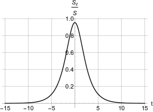
Figure 1: The normalized z spin component as a function of the proper time. We see that when the magnitude of the proper time is much greater than one, then we have a universe which is either exponentially contracting or expanding. However, these two different solution branches are connected by a regime, where the phase space curvature effects dominate. In this plot we have chosen initial conditions such that $S_{y}/S=0.3$, and $\hbar/S=10^{-10}$. $\hbar$ being much less than $S$ puts us well into the perturbative regime and we can expect the numerical solutions for the classical coordinates to be close to the analytic solutions. Moreover, at the point of recollapse we have $S_{x}=0$ and $\Delta(S_{y}^{2})=\frac{1}{2}\hbar S$. The adiabatic condition then fixes all other initial values.

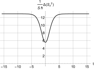
Figure 2: Fluctuation of $S_{z}$ given our initial conditions as a function of the proper time. We notice a sharp decrease in the magnitude of the fluctuations close to the point of recollapse, contrary to what would be expected in a model with a flat phase space. Again, we are in the semiclassical regime because we have chosen $\hbar/S=10^{-10}$. This then implies that the we are in a regime where the quantum numbers are large because: $S^{2}\sim s(s+1)\hbar^{2}$. This choice of initial conditions leads to moments that are parametrically small, and we can expect the corrections they give to be small. According to the discussion in (IV.5) we have chosen $\Delta(S_{y}^{2})=\frac{1}{2}\hbar S$. After that the adiabatic condition fixes all other initial values at the point of recollapse.

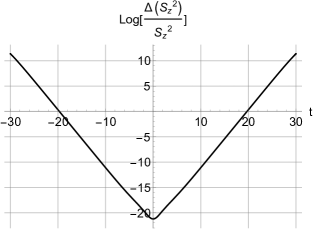
Figure 3: Logarithm of the relative fluctuations relative to the proper time. The relative fluctuations are the smallest towards the point of recollapse, and grow exponentially as the universe shrinks in size. The quantum corrections therefore become dominant at a certain time in the early universe. For this plot we have chosen the same initial conditions as in Fig: 2

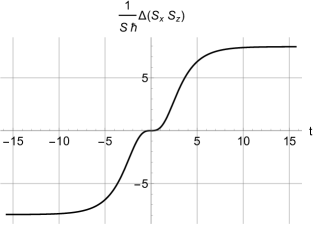
Figure 4: Correlation function between $S_{x}$ and $S_{z}$ as a function of the proper time. Even though this correlation is zero at the point of recollapse for adiabatic initial conditions we see that nontrivial correlations can develop during the evolution. Again, we have chosen the same initial conditions as in Fig: 2

IV.4 Effective Friedmann equations

For phenomenological purposes it is important to derive a Friedmann equation which receives not only corrections from the phase space curvature, but also from the quantum corrections, which can have important phenomenological applications. We can use the equation of motion for $S_{z}$ to derive such an equation. Moreover, we can use our solutions for the moments and classical spins to express $S_{z}^{\prime}$ in terms of only classical spins, or constants of motion. The equation of motion for $S_{z}$ is only corrected by the moment $\Delta(S_{x}S_{y})$. Happily, this moment can be expressed in terms of the classical coordinates and the constants of motion:

$$\Delta(S_{x}S_{y})=-S_{x}S_{y}\left(1-\frac{S_{z}}{S_{x}}\arctan{\left(\frac{S_{x}}{S_{z}}\right)}\right)\epsilon,$$ (36)

where for the later convenience we have introduced parametrized relative quantum fluctuations of $S_{y}$ by the parameter $\epsilon$ defined in Eq. 32.

We can now insert this solution into the equation of motion for $S_{z}$. We obtain:

$$S^{\prime}_{z}=-2S_{y}S_{x}\left[1-\left(1-\frac{S_{z}}{S_{x}}\arctan{\left(\frac{S_{x}}{S_{z}}\right)}\right)\epsilon\right].$$ (37)

Next, we perform a transformation back to the proper time, in order to make contact with the proper time Hubble factor. We obtain,

$$\dot{S}_{z}=-2S_{y}S_{x}S_{z}\left[1-\left(1-\frac{S_{z}}{S_{x}}\arctan{\left(\frac{S_{x}}{S_{z}}\right)}\right)\epsilon\right].$$ (38)

We now undo the time reparametrization that we performed at the beginning of our analysis:

$$\dot{S}_{z}=-\frac{3}{2}\frac{\kappa S_{y}S_{x}S_{z}}{R_{1}R_{2}^{2}}\left[1-\left(1-\frac{S_{z}}{S_{x}}\arctan{\left(\frac{S_{x}}{S_{z}}\right)}\right)\epsilon\right].$$

From the expression of $S_{z}$ (7), this implies that

$$\dot{q}=\frac{3}{2}\frac{\kappa}{S^{2}}\frac{S_{x}S_{y}S_{z}}{\cos{(q/R_{2})}}\left[1-\left(1-\frac{S_{z}}{S_{x}}\arctan{\left(\frac{S_{x}}{S_{z}}\right)}\right)\epsilon\right],$$

agreeing with the kinematical Hubble factor (14), in the limit $\hbar\rightarrow 0$. Furthermore, we can express the Hubble parameters in terms of $q$ only:

$$H^{2} =N^{2}\frac{\Lambda}{3}\left(\frac{\sin{(q/R_{2})}}{q/R_{2}}\right)^{2}\left[\frac{\cos{(q/R_{2})^{2}}-\delta}{\cos{(q/R_{2})^{2}}}\right]$$

$$\times\Big{[}1-2\epsilon\mathcal{F}(q)\Big{]}.$$ (39)

The pre-factor matches with what is found in the classical case, and the post factor contains quantum corrections, parametrized by the relative quantum fluctuations $\epsilon$. The function $\mathcal{F}(q)$ is given by:

$$\mathcal{F}(q)=1-\frac{\sin{(q/R_{2})}\arctan{\left(\frac{\sqrt{\cos{{}^{2}(q/R_{2})}-\delta}}{\sin{(q/R_{2})}}\right)}}{\sqrt{\cos{{}^{2}(q/R_{2})}-\delta}}.$$ (40)

This function encodes the behavior of the semiclassical corrections.

Taking the small phase space curvature limit we can make the approximation $\mathcal{F}\approx 1-\frac{\pi}{2\sqrt{1-\delta}}\frac{q}{R_{2}}$. Furthermore, the entire Hubble parameter can be expressed in the small phase space curvature limit.

$$H^{2}=N^{2}\frac{\Lambda}{3}\left[1-\delta-2\left[1-\frac{\pi}{2\sqrt{1-\delta}}\frac{q}{R_{2}}\right]\epsilon\right],$$ (41)

The quantum effects therefore weaken the gravitational attraction at sufficiently small volumes, which is expected based on the expectation that quantum effects should make gravity repulsive at Planckian densities. As a possible phenomenological implication, we notice that in this limit, the quantum corrections contain a term that is proportional to the volume. The quantum corrected non linear phase space therefore predicts that there is a negative jerk, which can in principle be measured. However, to make an accurate prediction for this jerk, we would need to make our model more realistic by including other types of matter, as well as perturbations, going beyond the minisuperspace approximation.

IV.5 Cosmological NFST in the $\mathcal{C}_{3}=0$ case

In order to justify some of our choices for initial conditions, and to gain some physical intuition for the physical evolution of our spin system, we consider the case where $\mathcal{C}_{3}=0$ such that we project our wavepacket on to a surface of constant spin, which is in turn equivalent to restricting our system to eigenstates of $\hat{S}^{2}$.

One way to implement this reduced system is to introduce a constraint to our semiclassical Hamiltonian. An alternative way, which gives more physical intuition, is to realize the spin algebra in terms of Casimir-Darboux coordinates, and then to quantize the resulting canonical variables. Such a canonical parametrization is given by:

$$\begin{split}S_{x}&=\sqrt{S^{2}-p_{\alpha}^{2}}\sin{\alpha},\\ S_{y}&=p_{\alpha},\\ S_{z}&=\sqrt{S^{2}-p_{\alpha}^{2}}\cos{\alpha}.\end{split}$$ (42)

Where we have $\left\{\alpha,p_{\alpha}\right\}=1$. It can be verified that this parametrization obeys the original bracket: $\left\{S_{i},S_{j}\right\}=\epsilon_{ijk}S_{k}$. By allowing $\alpha$ and $p_{\alpha}$ to fluctuate, we can relate fluctuations of the spin into fluctuations of these canonical coordinates.

$$\begin{split}\hat{S}_{i}&=S_{i}+\delta\hat{S_{i}}\\ &=S_{i}\left[\alpha+\delta\hat{\alpha},p_{\alpha}+\delta\hat{p}_{\alpha}\right]\\ &\approx S_{i}\left[\alpha,p_{\alpha}\right]+\frac{\partial S_{i}}{\partial\alpha}\delta\hat{\alpha}+\frac{\partial S_{i}}{\partial p_{\alpha}}\delta\hat{p}_{\alpha}.\end{split}$$ (43)

This in turn implies:

$$\begin{split}\Delta(S_{y}^{2})&=\Delta(p_{\alpha}^{2}),\\ \Delta(S_{x}^{2})&=\left(S^{2}-p_{\alpha}^{2}\right)\cos{{}^{2}(\alpha)}\Delta(\alpha^{2})-\sin{(2\alpha)}p_{\alpha}\Delta(\alpha p_{\alpha})+\frac{p_{\alpha}^{2}}{S^{2}-p_{\alpha}^{2}}\sin{{}^{2}(\alpha)}\Delta(p_{\alpha}^{2}),\\ \Delta(S_{z}^{2})&=\left(S^{2}-p_{\alpha}^{2}\right)\sin{{}^{2}(\alpha)}\Delta(\alpha^{2})+\sin{(2\alpha)}p_{\alpha}\Delta(\alpha p_{\alpha})+\frac{p_{\alpha}^{2}}{S^{2}-p_{\alpha}^{2}}\cos{{}^{2}(\alpha)}\Delta(p_{\alpha}^{2}),\\ \Delta(S_{y}S_{z})&=-\frac{p_{\alpha}\cos{(\alpha)}}{\sqrt{S^{2}-p_{\alpha}^{2}}}\Delta(p_{\alpha}^{2})-\sqrt{S^{2}-p_{\alpha}^{2}}\sin{(\alpha)}\Delta(\alpha p_{\alpha}),\\ \Delta(S_{y}S_{x})&=-\frac{p_{\alpha}\sin{(\alpha)}}{\sqrt{S^{2}-p_{\alpha}^{2}}}\Delta(p_{\alpha}^{2})+\sqrt{S^{2}-p_{\alpha}^{2}}\cos{(\alpha)}\Delta(\alpha p_{\alpha}),\\ \Delta(S_{x}S_{z})&=-(S^{2}-p_{\alpha}^{2})\cos{(\alpha)}\sin{(\alpha)}\Delta(\alpha^{2})-p_{\alpha}\cos{(2\alpha)}\Delta(\alpha p_{\alpha})+\frac{p_{\alpha}^{2}}{S^{2}-p_{\alpha}^{2}}\cos{(\alpha)}\sin{(\alpha)}\Delta(p_{\alpha}^{2}).\end{split}$$ (44)

We then have the algebra:

$$\begin{split}\left\{\alpha,p_{\alpha}\right\}&=1,\\ \left\{S^{2},\bullet\right\}&=0,\\ \left\{\Delta(p_{\alpha}^{2}),\Delta(\alpha^{2})\right\}&=-4\Delta(\alpha p_{\alpha}),\\ \left\{\Delta(p_{\alpha}^{2}),\Delta(\alpha p_{\alpha})\right\}&=-2\Delta(p_{\alpha}^{2}),\\ \left\{\Delta(\alpha^{2}),\Delta(\alpha p_{\alpha})\right\}&=2\Delta(\alpha^{2}).\end{split}$$ (45)

Finally, things are most simple if we use a faithful canonical parametrization of the moment algebra:

$$\begin{split}\Delta(p_{\alpha}^{2})&=p_{\sigma}^{2}+\frac{U}{\sigma^{2}},\\ \Delta(p_{\alpha}\alpha)&=\sigma p_{\sigma},\\ \Delta(\alpha^{2})&=\sigma^{2}.\end{split}$$ (46)

The $U$ is the Casimir parameter of the algebra, which can be identified as the uncertainty of the canonical coordinates: $\Delta(p_{\alpha}^{2})\Delta(\alpha^{2})-\Delta(\alpha p_{\alpha})^{2}=U$. After this reduction of states, and the implementation of the canonical coordinate system we have the deparametrized Hamiltonian:

$$\begin{split}H_{Q}=S_{y}^{2}+\Delta(S_{y}^{2})=p_{\alpha}^{2}+p_{\sigma}^{2}+\frac{U}{\sigma^{2}}.\end{split}$$ (47)

Interpreting $\sqrt{U}$ as an angular momentum, we can identify this Hamiltonian as the Hamiltonian of a free particle in three dimensions written in cylindrical coordinates. Only the particle is not allow to get to close to the $\alpha$ axis, because the angular momentum is bounded from below by the Heisenberg uncertainty $\sqrt{U}\geq\hbar/2.$ This gives us some insight into the dynamics. For example, we expect $\sigma$ to grow without bound, and to generally only have one local minimum.

We can take things further by considering the eigenvalues and eigenvectors of the covariance matrix: $\Delta(S_{i}S_{j})$. These quantities are important because the allow us to most easily vizualize the evolution of the ellipsoid in the phase space. The covariance matrix is three dimensional, so in the general case we might not expect to obtain nice analytical solutions. However, because of the reduction we made to the case $\mathcal{C}_{3}=0$, we expect one of the eigenvalues to be zero, because the wave packet is flattened on to the sphere of constant spin. Explicit calculations give:

$$\begin{split}\lambda_{1}&=0,\\ \lambda_{2}&=\frac{1}{2(S^{2}-p_{\alpha}^{2})\sigma^{2}}\Big{[}S^{2}U+S^{2}\sigma^{2}p_{\sigma}^{2}+\left(S^{2}-p_{\alpha}^{2}\right)^{2}\sigma^{4}\\ &+\sqrt{S^{4}U^{2}+2p_{\sigma}^{2}S^{4}U\sigma^{2}+S^{2}\left(p_{\sigma}^{4}S^{2}-2(S^{2}-p_{\sigma}^{2})^{2}U\right)\sigma^{4}+2S^{2}p_{\sigma}^{2}\left(S^{2}-p_{\alpha}^{2}\right)^{2}\sigma^{6}+\left(S^{2}-p_{\alpha}^{2}\right)^{4}\sigma^{8}}\,\,\Big{]},\\ \lambda_{3}&=\frac{1}{2(S^{2}-p_{\alpha}^{2})\sigma^{2}}\Big{[}-S^{2}U-S^{2}\sigma^{2}p_{\sigma}^{2}-\left(S^{2}-p_{\alpha}^{2}\right)^{2}\sigma^{4}\\ &+\sqrt{S^{4}U^{2}+2p_{\sigma}^{2}S^{4}U\sigma^{2}+S^{2}\left(p_{\sigma}^{4}S^{2}-2(S^{2}-p_{\sigma}^{2})^{2}U\right)\sigma^{4}+2S^{2}p_{\sigma}^{2}\left(S^{2}-p_{\alpha}^{2}\right)^{2}\sigma^{6}+\left(S^{2}-p_{\alpha}^{2}\right)^{4}\sigma^{8}}\,\,\Big{]}.\end{split}$$ (48)

We remark that the only time dependent parameters in this expression are $\sigma$ and $p_{\sigma}$. Despite the complexity of these expressions, we have:

$$\lambda_{2}\lambda_{3}=US^{2}.$$ (49)

Indicating that the area of our wave packet on the sphere is conserved. Which is expected for semiclassical states evolving according to (47). Taylor expanding (48) for large $\sigma$ (or equivalently the late time limit), we find:

$$\begin{split}\lambda_{2}&\approx\frac{S^{2}}{S^{2}-p_{\alpha}^{2}}\left(p_{\sigma_{o}}^{2}+\frac{U}{\sigma_{0}^{2}}\right)+\left(S^{2}-p_{\alpha}^{2}\right)\sigma^{2},\\ \lambda_{3}&\approx\frac{S^{2}}{S^{2}-p_{\alpha}^{2}}\frac{U}{\sigma^{2}}.\end{split}$$ (50)

So generally the wave packet will be squeezed in one direction and stretched in the other, while remaining flat on the curved phase space, as one would expect from the case of a quantum particle evolving in flat two dimensional phase space.

Furthermore, this analysis allows us to obtain estimates for the initial conditions of the full quantum evolution. Starting with (49), we notice that for symmetric states we have $\lambda^{2}=US^{2}\geq\frac{1}{4}\hbar^{2}S^{2}$. Since, $\lambda$ is a good estimate for the size of the dispersions and because we will restrict ourselves to states that are not so extremely squeezed, we expect our initial moments to be of order $\hbar S$. It is therefore reasonable to take the initial condition: $\Delta(S_{y}^{2})/(\delta S^{2})=\epsilon\sim\hbar/(\delta S)$ in the full analysis where there is less analytic control. This epsilon parametrizes the quantum corrections in our model and therefore it is crucial that we make a good estimate for it. As noted below, $\epsilon$ is related to the relative fluctuations of the Hubble parameter and therefore we expect it to be very small.

In this reduced setting it is also instructive to consider the eigenvectors of the covariance matrix. Not surprisingly, the eigenvector with eigenvalue zero is $\nu_{1}=\vec{S}=\left(\sqrt{S^{2}-p_{\alpha}^{2}}\sin{(\alpha)},p_{\alpha},\sqrt{S^{2}-p_{\alpha}^{2}}\cos{(\alpha)}\right)$. In the late time limit, we find the other eigenvectors have the approximate form: $\nu_{2}=\frac{\partial\nu_{1}}{\partial\alpha}$ and $\nu_{3}=\frac{\partial\nu_{1}}{\partial p_{\alpha}}$. Therefore, the wavepacket is spreading out in the direction of the motion in the phase space and contracting in the direction perpendicular to the motion. We find that these qualitative features are reproduced when the full dynamics are taken into account.

V Phenomenology and Bousso bound

The results which have been presented in the previous sections show that semiclassical homogeneous and isotropic gravitational sector can be constructed with the use of a spin degree of freedom. This has relevance from the point of view of extracting cosmological sector from a general (inhomogeneous) configuration of quantum gravitational system. Let us discuss this issue by assuming that elementary degrees of freedom of gravitational field are two dimensional quantum systems (qubits). This assumption is not crucial, and any higher dimensional elementary degrees of freedom can be considered, however, qubits are the smallest non-trivial quantum systems to which any higher dimensional quantum system can be always reduced to. The qubits are also corresponding to fundamental representations (spin-1/2) of the $SU(2)$ theory, which are utilized in such approaches to quantum gravity as LQG.

Let us denote the Hilbert space of a qubit (spin-1/2) as $\mathcal{H}_{1/2}$, such that $\text{dim}\mathcal{H}_{1/2}=2$. Then, the Hilbert space of the system of $N$ qubits is

$$\mathcal{H}_{\text{tot}}=\bigotimes_{i=1}^{N}\mathcal{H}_{1/2},$$ (51)

and has dimension $\text{dim}\mathcal{H}_{\text{tot}}=2^{N}$. Without the lose of generality let us consider an even $N$. Then, the semiclassical homogenous and isotropic cosmological configuration is a state in a subspace $\mathcal{H}_{\text{cosm}}\subset\mathcal{H}_{\text{tot}}$ and is corresponding to the maximal spin. The maximal spin $s_{\text{max}}$, in the system of $N$ spins $1/2$ is $s_{\text{max}}=N/2$, such that

$$\mathcal{H}_{\text{cosm}}=\mathcal{H}_{s_{\text{max}}},$$ (52)

and $\text{dim}\mathcal{H}_{\text{cosm}}=2s_{\text{max}}+1=N+1$. Then, the total Hilbert space can be decomposed as follows $\mathcal{H}_{\text{tot}}=\mathcal{H}_{\text{cosm}}\otimes\mathcal{H}_{\text{inh}}$, where $\mathcal{H}_{\text{inh}}$ is the Hilbert space of the inhomogeneous sector having dimension:

$$\text{dim}\mathcal{H}_{\text{inh}}=2^{N}-(N+1).$$ (53)

The spin $S$ present in our previous considerations can be now interpreted as $S=\hslash\sqrt{s_{\text{max}}(s_{\text{max}}+1)}\approx\hslash s_{\text{max}}=\frac{\hslash}{2}N$. So the higher the number of degrees of freedom $N$ the bigger $S$ and in consequence, the spin description is closer to the standard case of GR.

Based on the above considerations one can observe that, because cosmological sector is dependent on the parameter $S$, which in turn is a function of the total number of degrees of elementary freedom $N\sim S/\hslash$, analysis of the minisuperspace configuration allows to constrain the total number of degrees of freedom which are involved. Such analysis is especially interesting from the perspective of the constraint on the number of degrees of freedom in the Hubble volume implied by the holographic principle Susskind:1994vu and the holographic Bousso bound Bousso:1999xy ; Bousso:2002ju .

In the cosmological context, the holographic bound claims that the number of degrees of freedom in the Hubble volume $V_{\text{H}}$ - which we call $N_{\text{bulk}}$ - does not exceed the number of degrees of freedom at the boundary of the volume (which is the Hubble area $A_{\text{H}}$). By denoting the number of degrees of freedom at the Hubble area as $N_{\text{boundary}}$, the Bousso bound can be stated as:

$$N_{\text{bulk}}\leq N_{\text{boundary}}.$$ (54)

While such inequality is satisfied, the bulk can be unambiguously described by the information at the boundary, realizing the holographic principe.

In order to answer if our considerations allow to tell something about the condition (54), let us consider the parameter (32), which appeared in the modified Friedmann equation (39). In the, semiclassical limit, far from the deep Planckian regime, where $p\ll R_{1}$ and $q\sim R_{2}$ (so we are still far from the turning point), we have $S_{y}\approx\frac{S}{R_{1}}p$ (see Eq. 7), which allows us to approximate Eq. 32 as

$$\epsilon=\frac{\Delta(S_{y}^{2})}{S_{y}^{2}}\approx\frac{\Delta(p^{2})}{p^{2}}\approx\frac{\Delta(H^{2})}{H^{2}}.$$ (55)

The estimation of the relative fluctuations of the Hubble parameter is rather subtle. In what follows we will present an approach to the problem, which employs Planck scale fluctuations of the Hubble horizon

Namely, we can make an estimation of the relative fluctuations of the Hubble parameter, by changing variables to the Hubble radius $R_{\text{H}}:=1/H$, so that

$$\begin{split}\Delta(H^{2})&:=\Big{\langle}\left(\hat{H}-H\right)^{2}\Big{\rangle}=\Big{\langle}\left(\frac{1}{\hat{R}_{\text{H}}}-\frac{1}{R_{\text{H}}}\right)^{2}\Big{\rangle}\\ &=\Big{\langle}\left(\frac{1}{R_{\text{H}}+\widehat{\delta R_{\text{H}}}}-\frac{1}{R_{\text{H}}}\right)^{2}\Big{\rangle}\\ &=\frac{1}{R_{\text{H}}^{4}}\Big{\langle}\left(\widehat{\delta R_{\text{H}}}\right)^{2}\Big{\rangle}+O(\hbar^{{\color[rgb]{0,0,0}3/2}})\\ &\approx\frac{1}{R_{H}^{2}}\frac{\Delta(R_{\text{H}}^{2})}{R_{\text{H}}^{2}}=H^{2}\frac{\Delta(R_{\text{H}}^{2})}{R^{2}_{\text{H}}}.\end{split}$$ (56)

This implies that $\epsilon\approx\frac{\Delta(H^{2})}{H^{2}}\approx\frac{\Delta(R_{\text{H}}^{2})}{R^{2}_{\text{H}}}$. A reasonable assumption seem to be that quantum fluctuations of the Hubble horizon are tiny and of the order of the Planck length $l_{\text{Pl}}\approx 1.62\cdot 10^{-35}$ m. Therefore, the standard deviation $\sigma(R_{\text{H}}):=\sqrt{\Delta(R_{\text{H}}^{2})}\sim l_{\text{Pl}}$. Using this, as well as the fact that for de Sitter universe $R_{\text{H}}=\sqrt{\frac{3}{\Lambda}}$ (which is approximately satisfied in the case considered here), we can estimate that:

$$\epsilon\approx\frac{\Delta(S_{y}^{2})}{\delta S^{2}}\approx\frac{\Delta(R_{\text{H}}^{2})}{R^{2}_{\text{H}}}\sim l^{2}_{\text{Pl}}\Lambda,$$ (57)

where in the first approximation the equation of constraint $S_{y}^{2}\approx\delta S^{2}$ has been used. Taking the current values of the Hubble factor $H_{0}=67.8\pm 0.9\frac{\text{km}}{\text{s}\cdot\text{Mpc}}$ Ade:2015xua and the parameter $\Omega_{\Lambda}=\frac{\Lambda}{3H_{0}^{2}}=0.69\pm 0.01$ Ade:2015xua we can estimate that:

$$\epsilon\sim 10^{-122}.$$ (58)

Assuming that the momentum compactification scale (related to $R_{1}$) is Planckian, as one might expect from results in LQG, implies that $\rho_{c}\sim\rho_{\text{Pl}}:=m^{4}_{\text{Pl}}$. In consequence,

$$\delta:=\frac{\rho_{\Lambda}}{\rho_{c}}\sim\frac{\rho_{\Lambda}}{\rho_{\text{Pl}}}\sim l^{2}_{\text{Pl}}\Lambda\sim\epsilon.$$ (59)

Furthermore, from Sec. IV.5 we have the estimate, $\Delta{S_{y}^{2}}=\frac{1}{2}\hbar S$, which together with Eq. 59, allows us to rewrite Eq. 57 into

$$\frac{S}{\hbar}\sim\frac{1}{\epsilon^{2}}\sim 10^{224},$$ (60)

where the numerical value corresponds to the current estimate, employing Eq. 58. As discussed earlier in this section, the value of $S$ can give an estimate for the number of degrees of freedom in the bulk, i.e. $S\sim N_{\text{bulk}}\hslash$. Based on this we find, $N_{\text{bulk}}\sim 1/\epsilon^{2}\sim 10^{224}$.

On the other hand, the number of degrees of freedom at the boundary (Hubble horizon) can be estimated by dividing the area of the Hubble horizon, by the Planck cells of the area $l^{2}_{\text{Pl}}$ Artymowski:2018pyg :

$$N_{\text{boundary}}\approx\frac{A_{\text{H}}}{l^{2}_{\text{Pl}}}=\frac{4\pi R^{2}_{\text{H}}}{l^{2}_{\text{Pl}}}\sim\frac{1}{l^{2}_{\text{Pl}}\Lambda}\sim\frac{1}{\epsilon}\sim 10^{122}.$$ (61)

Therefore, in the considered case:

$$N_{\text{bulk}}\sim N_{\text{boundary}}^{2},$$ (62)

and the number of degrees of freedom in the bulk is much greater than those on the boundary, violating the holographic Bousso bound (54).

In order to satisfy the Bousso bound we might try to generalize our estimate of $\Delta(S_{y}^{2})$. We only have two parameters with dimension of action, so we can consider the power-law ansatz: $\Delta(S_{y}^{2})\sim\hbar^{2}(S/\hslash)^{k}$, where $k\leq 2$. The upper bound on the values of $k$ comes from the fact that the relative fluctuations $\frac{\Delta(S_{y}^{2})}{S^{2}}\sim(S/\hslash)^{k-2}$, and the values $k>2$ imply lack of semiclassicality of the state. For $k=1$ the previously case, violating the Bousso bound, is recovered. Another spacial case is $k=0$, which implies $\Delta(S_{y}^{2})\sim\hbar^{2}$ and corresponds to a strongly squeezed state. For $k<0$, while the relative fluctuations of $S_{y}$ decrease with the increase of $S$ (guaranteeing semiclassicality), the squeezing of state is very large, which has to be balanced by a large fluctuations of the other spin components. Therefore, while the despite the $k<0$ satisfies the Bousso bound, since we have

$$N_{\text{bulk}}\sim N_{\text{boundary}}^{\frac{2}{2-k}},$$ (63)

with the power $\frac{2}{2-k}<1$, such case is rather disfavored on the physical ground. The remaining case is $k=0$, for which

$$N_{\text{bulk}}\sim N_{\text{boundary}},$$ (64)

and the Bousso bound has chance to be satisfied by a proper choice of the proportionality factor.

Concerning the issue of semiclassicality for the $k=0$ case, let us resort to our analysis of the quantum fluctuations of the undeformed spherical phase space, presented in Sec. IVE. This is a reasonable case, especially if we assume that the state is condensing in the $S=s_{\text{max}}\hbar$ sector of the Hilbert space. The squeezing with $k=0$ implies $\Delta(p_{\alpha}^{2})\sim\hbar^{2}$, but then the Heisenberg uncertainty principle for canonical variables implies: $\Delta(\alpha^{2})\sim 1$. Given our canonical mapping this implies: $\frac{\Delta(S_{x}^{2})}{S^{2}}\sim\frac{\Delta(S_{z}^{2})}{S^{2}}\sim 1$. The character of such a state which is squeezed and satisfies the Bousso bound, is therefore not semiclassical.

VI Summary

In summary, our semiclassical analysis of a de Sitter model with a compact ($\mathbb{S}^{2}$) phase space has given us insight into the behavior of the quantum fluctuations in the model. In particular, we were able to find analytic solutions for the leading order moment corrections, despite the non-linearity of the effective system. These analytic solutions agree well with standard results of quantum fluctuations in a de-Sitter model with a flat phase space, and make new predictions in the regime where the classical coordinates are the same order as the phase space radius of curvature. While qualitative, these predictions are interesting, and possibly indicate future research directions.

Unfortunately, it is hard to make concrete quantitative phenomenological predictions in this setting, due to the highly simplified nature of the model. However, our solutions for the semiclassical corrections do indicate several interesting qualitative predictions. For example, our solutions indicate that the classical variables would not be periodic in a cyclic universe, and in particular, these classical variables are resonating with the quantum corrections. The time constant for this resonance, is several lifetimes of the universe. Within this simplified setting of this model, this indicates the semiclassical states are not a stable variational class. A possible way around this issue would be to introduce different types of ordinary matter, or to include density perturbations. However, this would complicate the model, possibly making analytic solutions impossible to find.

Furthermore, our solutions have several qualitative features which could have phenomenological implications. Our calculation of the NFST Hubble parameter in the presence of quantum corrections indicates that there is a negative jerk which could become relevant before one would expect based on the classical NFST. Moreover, for the initial conditions under consideration, we observe a sharp decrease in the quantum fluctuations close to the point of recollapse.

Finally, the obtained results are discussed from the perspective of the number of degrees of freedom involved in construction of the semiclassical cosmological state and the fate of the holographic principle. We find that the semiclassical state supported by the considerations presented in this article violates the Bousso bound. However, a state which may satisfy the holographic bound is still acceptable based on physical considerations. This opens an intriguing possibility to build a quantum (compact phase space) version of de Sitter model satisfying the Bousso bound.

References

- (1) M. Born, Rev. Mod. Phys. 21, 463 (1949).
- (2) A. Ashtekar and T. A. Schilling, gr-qc/9706069.
- (3) H. S. Snyder, Phys. Rev. 71, 38 (1947). doi:10.1103/PhysRev.71.38
- (4) S. Majid, Lect. Notes Phys. 541, 227 (2000) [hep-th/0006166].
- (5) A. Connes, “Noncommutative geometry,”
- (6) G. Amelino-Camelia, L. Freidel, J. Kowalski-Glikman and L. Smolin, Phys. Rev. D 84, 084010 (2011) [arXiv:1101.0931 [hep-th]].
- (7) G. Amelino-Camelia, L. Freidel, J. Kowalski-Glikman and L. Smolin, Gen. Rel. Grav. 43, 2547 (2011) [Int. J. Mod. Phys. D 20, 2867 (2011)] [arXiv:1106.0313 [hep-th]].
- (8) A. Ashtekar and J. Lewandowski, Class. Quant. Grav. 21 (2004) R53 [gr-qc/0404018].
- (9) C. Rovelli, Living Rev. Rel. 1 (1998) 1 [gr-qc/9710008].
- (10) M. Bojowald, Living Rev. Rel. 11 (2008) 4.
- (11) M. Bojowald, Phys. Rev. Lett. 86, 5227 (2001) doi:10.1103/PhysRevLett.86.5227 [gr-qc/0102069].
- (12) C. Rovelli and F. Vidotto, “Covariant Loop Quantum Gravity : An Elementary Introduction to Quantum Gravity and Spinfoam Theory,”
- (13) A. Riello, Phys. Rev. D 97, no. 2, 025003 (2018) [arXiv:1706.07811 [hep-th]].
- (14) B. Dittrich, JHEP 1705, 123 (2017) [arXiv:1701.02037 [hep-th]].
- (15) H. M. Haggard, M. Han and A. Riello, Annales Henri Poincare 17, no. 8, 2001 (2016) [arXiv:1506.03053 [math-ph]].
- (16) J. Mielczarek and T. Trześniewski, Phys. Lett. B 759, 424 (2016), [arXiv:1601.04515 [hep-th]].
- (17) J. Bilski, S. Brahma, A. Marcianò and J. Mielczarek, Int. J. Mod. Phys. D 28, no. 01, 1950020 (2018) [arXiv:1708.03207 [hep-th]].
- (18) J. Mielczarek and T. Trześniewski, Phys. Rev. D 96, 043522 (2017).
- (19) M. Born and L. Infeld, Proc. R. Soc. A 144, 425 (1934).
- (20) J. Mielczarek, Universe 3, 29 (2017), [arXiv:1612.04355 [hep-th]].
- (21) D. Artigas, J. Mielczarek and C. Rovelli, Phys. Rev. D 100, no. 4, 043533 (2019) [arXiv:1904.11338 [gr-qc]].
- (22) J. Mielczarek and W. Piechocki, Phys. Rev. D 82, 043529 (2010), [arXiv:1001.3999 [gr-qc]].
- (23) I. Agullo and A. Corichi, doi:10.1007/978-3-642-41992-8_39 [arXiv:1302.3833 [gr-qc]].
- (24) A. Ashtekar, T. Pawlowski and P. Singh, Phys. Rev. D 74 (2006) 084003 [gr-qc/0607039].
- (25) J. Mielczarek, T. Stachowiak and M. Szydlowski, Phys. Rev. D 77 (2008) 123506 [arXiv:0801.0502 [gr-qc]].
- (26) J. Mielczarek and W. Piechocki, Phys. Rev. D 82 (2010) 043529 [arXiv:1001.3999 [gr-qc]].
- (27) P. Dzierzak, P. Malkiewicz and W. Piechocki, Phys. Rev. D 80, 104001 (2009) [arXiv:0907.3436 [gr-qc]].
- (28) C. Rovelli, doi:10.1017/CBO9780511755804
- (29) M. Bojowald, “Canonical Gravity and ApplicationsCosmology, Black Holes, and Quantum Gravity,”
- (30) B. Baytas and M. Bojowald, Phys. Rev. D 95, no. 8, 086007 (2017) [arXiv:1611.06255 [gr-qc]].
- (31) Bojowald, Martin and Sandh’́o fer, Barbara and Skirzewski, Aureliano and Tsobanjan, Artur, Rev. Math. Phys. 21 (2009) 111-154
- (32) L. Susskind, J. Math. Phys. 36 (1995) 6377 [hep-th/9409089].
- (33) R. Bousso, JHEP 9907 (1999) 004 [hep-th/9905177].
- (34) R. Bousso, Rev. Mod. Phys. 74 (2002) 825 [hep-th/0203101].
- (35) P. A. R. Ade et al. [Planck Collaboration], Astron. Astrophys. 594 (2016) A13 [arXiv:1502.01589 [astro-ph.CO]].
- (36) M. Artymowski and J. Mielczarek, Eur. Phys. J. C 79 (2019) no.7, 632 [arXiv:1806.03924 [gr-qc]].