Computation of Tight Enclosures for
Laplacian Eigenvalues

Abstract.

Recently, there has been interest in high-precision approximations of the first eigenvalue of the Laplace-Beltrami operator on spherical triangles for combinatorial purposes. We compute improved and certified enclosures to these eigenvalues. This is achieved by applying the method of particular solutions in high precision, the enclosure being obtained by a combination of interval arithmetic and Taylor models. The index of the eigenvalue is certified by exploiting the monotonicity of the eigenvalue with respect to the domain. The classically troublesome case of singular corners is handled by combining expansions at all corners and an expansion from an interior point. In particular, this allows us to compute 100 digits of the fundamental eigenvalue for the 3D Kreweras model that has been the object of previous efforts.

Introduction

The most classical situation for the computation of Laplacian eigenvalues is that of the Laplacian on a bounded open set $\Omega\subset\mathbb{R}^{d}$. There is an increasing sequence $(\lambda_{n})_{n}$ of positive real numbers, called the eigenvalues, and corresponding (eigen)functions $(u_{n})_{n}$ in $C^{\infty}(\Omega)$ such that $\Delta u_{n}+\lambda_{n}u_{n}=0$ in $\Omega$, while $u_{n}=0$ on the boundary $\partial\Omega$ (a Dirichlet condition). Moreover, $(u_{n})$ is a Hilbert basis of $L^{2}(\Omega)$ (see, e.g., [17, 15]). The method of particular solutions was introduced by Fox, Henrici and Moler [22] and later refined by Betcke and Trefethen [9]. Betcke [8] describes this method as “especially effective for very accurate computations”. (He also gives pointers to precursors and related works.) Starting from a solution $u^{*}$ of $\Delta u+\lambda^{*}u=0$ in $\Omega$ for some $\lambda^{*}$ that does not necessarily satisfy $u^{*}|_{\partial\Omega}=0$, this method lets one deduce an interval around $\lambda^{*}$ that contains an eigenvalue of the original problem and whose diameter can be bounded in terms of $\max_{x\in\partial\Omega}|u^{*}(x)|$ and $\|u^{*}\|_{2}$. The candidate pair $(\lambda^{*},u^{*})$ is computed by first finding a set $(f_{n,\lambda})$ of solutions of $\Delta u+\lambda u=0$ in $\Omega$; next, looking for a linear combination of unit norm which is minimal on the boundary; finally looking for $\lambda$ where this minimum value is close to 0. For the prototypical example of the L-shaped region in the plane (displayed in Figure 1 on p. 1), Fox, Henrici and Moler could compute 5 certified digits of $\lambda_{1}$ with their method, using $10$ terms of the linear combination and further tricks exploiting the symmetry of the domain. With their improved method, Betcke and Trefethen produced 14 digits of $\lambda_{1}$ and certified 13 of them, without having to exploit any special feature and using 60 terms of the linear combination. In higher precision, this nice behaviour persists, as already observed by Jones [28]. We show how certifying an enclosure is also possible: these 14 digits can be certified with 100 terms of the expansion. The width of the enclosure scales well: using 180 terms gives 27 certified digits (see Section 2.5).

A corner of a polygonal domain in the plane is called regular if it has an angle on the form $\pi/k$ for some nonnegative integer $k$; corners with angles not of that type are called singular. The regularity of a corner results in eigenfunctions that can be continued analytically in a neighborhood of the corner by a reflection argument [17, V§16.6]. The L-shaped region in the plane is an example of a region with only one singular corner (the reentrant one). This is a favorable situation for the method: the expansion at the singular corner has no difficulty converging at the other ones. By the same reflection argument, a similar phenomenon takes place in the case of spherical triangles. This lets us improve upon previous work in this setting for triangles with at most one singular corner.

For polygonal domains with several singular corners, Betcke and Trefethen [9] used expansions at all the singular corners. In our experiments with spherical triangles, this technique alone has not been sufficient to make the method converge. However, there are known cases when, in different methods, joining data from the corners with data from the interior of the domain is successful [40, 24]. This also happens in our situation, where we have observed that taking expansions at all singular corners and complementing them with an expansion at an interior point worked very well. That is how we could compute 100 digits for the triangle with angles $(2\pi/3,2\pi/3,2\pi/3)$, see Section 3.9.

Combinatorial motivation

Recently, these computations have become relevant in the very active study of discrete walks in $\mathbb{N}^{d}$ (see recent surveys [29, 13] for numerous references). The relation between the Brownian motion and the heat equation can be exploited to derive the asymptotic number of walks in $\mathbb{N}^{d}$ starting and ending at the origin and using $n$ steps, all taken from a given finite set $S\subset\mathbb{Z}^{d}$ [18]. Under mild conditions, this number behaves asympotically like

(1) $$f_{S}(n)\sim K\rho^{n}n^{\alpha},\quad\alpha=-1-\sqrt{\lambda_{1}+(d/2-1)^{2}},$$

where $\lambda_{1}$ is the first eigenvalue (called the fundamental eigenvalue) of the Laplace-Beltrami operator on the sphere $\mathbb{S}^{d-1}$, with Dirichlet boundary conditions 0 on a spherical cone that can be computed from the step set $S$ (the constant $\rho$, which is more important asymptotically, can also be computed from $S$). A question of interest in combinatorics is the nature of the sequence $f_{S}(n)$, i.e., the type of recurrence it may satisfy. Depending on the step set $S$, it can be solution of a linear recurrence with constant coefficients, or with polynomial coefficients, or of no such recurrence. The asymptotics above can be used to rule out possibilities. For instance, if $f_{S}(n)$ satisfies a linear recurrence with constant coefficients, then the exponent $\alpha$ has to be a nonnegative integer. A deeper result is that if this integer sequence satisfies a linear recurrence with polynomial coefficients, then $\alpha$ has to be rational. This has been used to complete the classification of planar lattice walks with small steps (steps in $\{0,\pm 1\}^{2}$) [14]. It revealed a strong connection between the existence of a linear recurrence with polynomial coefficients and the finiteness of a group associated to the walk.

In dimension 3, an open question is whether the connection between linear recurrences and finiteness of the associated group still holds. Recently, Bogosel et alii established that the cases where the group is finite correspond to 17 triangles tiling the sphere that they give explicitly [12]. Of these, 7 triangles correspond to the small number of spherical triangles with three regular corners for which the eigenvalues of the Laplace-Beltrami operator are known explicitly [6, 7]. For the remaining 10 cases, only numerical approximations are available. Obviously, from a numerical estimate of the fundamental eigenvalue $\lambda_{1}$, one cannot expect to obtain a guarantee of the rationality of the related exponent $\alpha$ in Eq. (1). Instead, our aim is to use this numerical approximation as a filter by giving a lower bound on the size the denominator would have if the exponent was a rational number; small bounds would suggest the need for further combinatorial investigation. Thus, this is a situation where we are interested in computing tens or, ideally, hundreds of digits of the fundamental eigenvalue of the Laplace operator .

Certified computation

Eigenvalues of self-adjoint operators and their computation form a classical topic of numerical analysis; good surveys are available [31, 11, 25, 45].

The possible influence of rounding errors in the computation of bounds for eigenvalues leads naturally to the use of interval arithmetic in certified computations. The development of methods that are most suitable in this context started in the 1990’s [41, 5, 38]. Since then, the theoretical aspects have been extended to more and more general equations; see the recent book by Nakao, Plum and Watanabe [37] for an account of the main methods. The case of the Laplace operator has been studied by Liu and Oishi [33]. They mention the method of particular solutions, but discard it because it does not guarantee the index of the eigenvalue. Instead, they construct explicit eigenvalue bounds from a finite element method.

Our contribution to this problem is to show how the method of particular solutions lends itself to certified computations: we detail the extra work required to certify an enclosure for the eigenvalues and their index and show that this is not the time-consuming part of the computation. Moreover, that method has the advantage that it can easily be used to obtain high-precision results, which is difficult by methods based on finite elements (see for instance the discussion at the end of [24]).

In order to compute an enclosure for the fundamental eigenvalue by the method of particular solutions, the first step is to use the method without worrying about certified computations: any approximate pair $(\lambda^{*},u^{*})$ will do. The difficulties at this stage are the same as in a classical computation, mainly the slow convergence in the presence of singular corners and the linear combinations of basis functions that are very close to 0 inside the domain and make the linear algebra problem ill-conditioned. Once these difficulties are overcome and such an approximation at high precision is obtained, and only then, we need a more careful computation when bounding the distance to an actual close-by eigenvalue so that the enclosure can be guaranteed. This is described in Section 2.

Finally, we also need to prove that the eigenvalue that has been produced is indeed the fundamental one. For the spherical triangles we study, this is done in Section 3.5, by exploiting the monotonicity property of eigenvalues with respect to the domain, certified roots of Ferrers functions and a variant of Sturm’s theorem.

Recent works

Three recent works are most directly related to ours.

Jones [28] uses the method of particular solutions in high precision for the computation of eigenvalues for polygons in the plane. In particular, he obtains 1 000 digits of the fundamental eigenvalue of the L-shaped region. The correct digits are obtained thanks to an empirical observation: the eigenvalues of the truncated problems obtained by taking $N$ points on the boundary alternate below and above the limiting value as $N$ increases. In our context of certified computation, we cannot rely on this heuristic approach. We revert to computing certified bounds on the maximum value on the boundary and the norm of approximate eigenfunctions.

Very recently, Gómez-Serrano and Orriols [23] have proved that three eigenvalues do not determine a triangle. For this, they used the method of particular solutions in the plane in a spirit very similar to ours. The main differences with our work is that we need much higher precision, that the triangles they are interested in do not have any regular corner and that we work on the sphere rather than on the plane. Also, they have to deal with many more triangles. Their way of lower bounding the norm of the candidate eigenfunction is extended to singular spherical triangles in Section 2.2.

The finite element method has the disadvantage that a large discretization is needed in order to get a good accuracy. However, together with extrapolation, this approach was used with success by Bogosel, Perrollaz, Raschel and Trotignon [12] in our problem. They compute approximations of the fundamental eigenvalue for all 17 spherical triangles corresponding to walks with finite groups. Their results are compared to ours in Tables 1, 2 below. We can vastly improve the precision they obtain, both for triangles with at most one singular corner and for more singular triangles.

Plan

In Section 1, we first recall the method of particular solutions. Then, in Section 2 we spell out the steps we use in the certification stage and illustrate these in detail in the classical case of the L-shaped region (§2.5). This example is presented in such a way that the same steps apply to the spherical triangles in Section 3. We then show how the index of the eigenvalue can be certified in Section 3.5. The results for the spherical triangles that had been considered by Bogosel et al. are then given (§3.6,§3.7) and in §3.8, we conclude by providing lower bounds on the denominators the corresponding exponents from Eq. (1) would have if they were rational numbers, the case of the 3D Kreweras model being detailed in Section 3.9.

1. Method of Particular Solutions

The starting point of the method is the following a posteriori bound. It allows one to enclose an eigenvalue by finding good approximations to the eigenfunction.

Theorem 1.

[22, 36] Let $\Omega\subset\mathbb{R}^{n}$ be bounded. Let $\lambda$ and $u$ be an approximate eigenvalue and eigenfunction—that is, they satisfy $\Delta u+\lambda u=0$ in $\Omega$ but not necessarily $u=0$ on $\partial\Omega$. Define

$$\epsilon=\frac{\sqrt{\operatorname{Vol}(\Omega)}\sup_{x\in\partial\Omega}|u(x)|}{\|u\|_{2}}.$$

Then there exists an eigenvalue $\lambda_{*}$ such that

(2) $$\frac{|\lambda-\lambda_{*}|}{\lambda_{*}}\leq\epsilon.$$

Variants of this result hold more generally for elliptic differential operators. As stated here, the bound is due to Moler and Payne [36], improving upon the original bound by Fox, Henrici and Moler [22]. Further generalizations and improvements to this bound are available in the literature [31, 44, 4, 45].

The version of the method of particular solutions we give here is due Betcke and Trefethen [9, 8]. The starting point is a set of solutions $u_{\lambda}^{(k)}$ to $\Delta u+\lambda u=0$ in $\Omega$, that are not constrained on the boundary $\partial\Omega$. An approximate eigenfunction is given by a linear combination of these,

$$u_{\lambda}^{*}=\sum_{k=1}^{N}c_{k}u_{\lambda}^{(k)},$$

where the coefficients are chosen so that it is close to unit norm in $\Omega$ and minimal on the boundary.

The coefficients $c_{k}$ are found by taking $m_{B}$ points on the boundary, $\{x_{i}\}_{i=1}^{m_{B}}\subset\partial\Omega$, on which we want to minimize $u_{\lambda}^{*}$. This alone is not sufficient: increasing the number $N$ of elements in the basis leads to the existence of linear combinations very close to 0 inside the domain $\Omega$. These linear combinations lead to spurious solutions, even away from an eigenvalue. Betcke and Trefethen cure this problem by also considering $m_{I}$ points in the interior $\{y_{j}\}_{j=1}^{m_{I}}\subset\Omega$ and using them to make sure that the linear combinations of interest stay close to unit norm in the domain. The computation now involves two matrices

$$(A_{B})_{ik}(\lambda) =u^{(k)}_{\lambda}(x_{i}), 1\leq i\leq m_{B},\ 1\leq k\leq N;$$

$$(A_{I})_{jk}(\lambda) =u^{(k)}_{\lambda}(y_{j}), 1\leq j\leq m_{I},\ 1\leq k\leq N.$$

The matrices $A_{B}$ and $A_{I}$ can be combined into a matrix whose $QR$ factorization gives an orthonormal basis of these function evaluations

(3) $$A(\lambda)=\begin{bmatrix}A_{B}(\lambda)\\ A_{I}(\lambda)\end{bmatrix}=\begin{bmatrix}Q_{B}(\lambda)\\ Q_{I}(\lambda)\end{bmatrix}R(\lambda)=:Q(\lambda)R(\lambda).$$

Now, the right singular vector $v$ of norm 1 corresponding to the smallest singular value $\sigma(\lambda)$ of the top part $Q_{B}(\lambda)$ is a good candidate for the eigenfunction when $\sigma(\lambda)$ is small. Moreover,

$$\|Q(\lambda)v\|_{2}^{2}=1=\sigma(\lambda)^{2}+\|Q_{I}(\lambda)v\|^{2},$$

forcing the function to have norm close to 1 on the interior points. Thus the next step of the method is to search for $\lambda$ minimizing $\sigma(\lambda)$. Once such a $\lambda$ is found, the actual vector $c$ of coefficients is recovered by solving the linear system $R(\lambda)c=v$. As noted by Betcke and Trefethen this linear system is highly ill-conditioned but the solutions obtained are nevertheless small on the boundary of the domain. We observe the same phenomenon in our computations, taking place at a lot higher precision. Computing the minimum to a certain precision only requires 10-20 extra bits of precision in the intermediate computations even for as high as 300 bits of precision for the minimum.

Furthermore, Betcke and Trefethen give a geometric interpretation of $\sigma(\lambda)$: it is the sine of the angle between the subspace of $\mathbb{R}^{m_{B}+m_{I}}$ generated by the columns of $A$ — the values of the functions $(u_{\lambda}^{(k)})$ at the interior and boundary points $x_{i}$ and $y_{i}$ — and the subspace $\mathbb{R}^{m_{B}}\times 0^{m_{I}}$ — the values of functions that are 0 at the boundary points $y_{i}$. This angle becomes 0 when these spaces intersect, which means that a combination of the functions $(u_{\lambda}^{(k)})$ is 0 at the boundary points $y_{i}$. Betcke shows that the tangent of that same angle is the smallest generalized singular eigenvalue of the pencil $\{A_{B},A_{I}\}$, which gives another way of computing it [8].

2. Certified computation of the enclosure

The method of particular solutions can be performed in high precision environments as provided by computer algebra systems or by specialized libraries like MPFR, but of course, running in high precision does not guarantee anything about the accuracy of the result. Given an approximate eigenfunction $u$, a certified enclosure of the eigenvalue is provided by Theorem 1 provided we obtain an upper bound on the maximum of $|u|$ on the boundary $\partial\Omega$ and a lower bound on its norm in $\Omega$.

As in the previous section, we let $u(x)$ be given by a linear combination of functions $u_{k}(x)$

$$u(x)=\sum_{k=1}^{N}c_{k}u_{k}(x).$$

The details of the implementation of the method depend on the actual family of functions $u_{k}(x)$ and on the domain. The following approach works in all our examples that are two-dimensional.

2.1. Upper bound on the boundary

This is the difficult part. A key role in certified computations is played by interval arithmetic [46, 26], but it cannot be applied blindly. The function $u(x)$ is given by a sum of individually large terms whose sum is expected to be very small on the boundary. A direct use of interval arithmetic is bound to fail, as it handles cancellations poorly. The technique of Taylor models [34] overcomes this difficulty: instead of bounding the function directly, one computes a Taylor expansion of the function before computing a bound by interval arithmetic. If $\gamma:[0,1]\rightarrow\partial\Omega$ is a parametrization of the boundary and $I\subset[0,1]$ is an interval of width $|I|$, then

$$\max_{t\in I}u(\gamma(t))\leq\max_{t\in I}P_{\ell-1}(t)+\frac{(|I|/2)^{\ell}}{\ell!}\max_{t\in I}\left|\frac{d^{\ell}}{dt^{\ell}}u(\gamma(t))\right|,$$

where $P_{\ell-1}$ is the Taylor polynomial of $u(\gamma(t))$ of order $\ell-1$ centered around the midpoint of the interval. Since the functions $u_{k}$ are obtained from the Laplacian by separation of variables, they satisfy linear differential equations from which linear recurrences for the Taylor coefficients follow. Thus the polynomial $P_{\ell-1}$ can be computed efficiently to high precision. Bounding it on the interval $I$ can be done by locating possible extrema using classical interval arithmetic. Bounding $\left|\frac{d^{\ell}}{dt^{\ell}}u(\gamma(t))\right|$ on the interval $I$ by interval arithmetic does suffer from the same problems as bounding $u(\gamma(t))$ directly. This is however mitigated by the factor ${(|I|/2)}^{\ell}/{\ell!}$, which can be made small by choosing a sufficiently large $\ell$ and/or a sufficiently small $|I|$.

Without any extra computational effort, this also gives a lower bound on the boundary as

$$\min_{t\in I}u(\gamma(t))\geq\min_{t\in I}P_{\ell-1}(t)-\frac{(|I|/2)^{\ell}}{\ell!}\max_{t\in I}\left|\frac{d^{\ell}}{dt^{\ell}}u(\gamma(t))\right|,$$

which can be used when lower bounding the norm below.

In the computations, $\ell$ is chosen to be the same as the number of terms in the expansion of $u$. This choice is heuristic but in practice this means that the number of subdivisions required stays approximately constant as the number of terms in $u$ increases. Due to the fact that there are a lot of cancellations, using sufficiently high precision in the computations is important. In practice we add 30 bits of precision for computations with a target precision of 100-300 bits, only the high precision computations of the Kreweras triangle in Section 3.9 require up to 80 extra bits of precision. Adding more precision is however rather cheap and we have favored using unnecessary bits over trying to minimize the number of bits used in intermediate computations.

2.2. Lower bound on the norm

This is easier as only the magnitude is needed and no cancellation takes place. The norm can be lower bounded by computing it on a subset of the domain, $\Omega^{\prime}\subset\Omega$. In our examples two different cases occur.

In the case when there is a single expansion in an orthogonal basis, it is natural to let $\Omega^{\prime}$ be a circular sector inside the domain. Then the integral giving the norm of $u(x)$ splits into a sum of one-dimensional integrals. These one-dimensional integrals can then be lower bounded by means of a verified integrator [27]. This is what we do for the L-shaped region below and in the case of regular triangles in Section 3.4.

When the terms in the expansion are not orthogonal, more work is required. We apply a method used by Gómez-Serrano and Orriols [23] in the context of polygons. The idea is that if $u$ does not vanish in a subset $\Omega^{\prime}$ of $\Omega$, without loss of generality it can be assumed to be positive there and then, since $-\Delta u=\lambda u>0$, $u$ is a superharmonic function and satisfies $\inf_{\Omega^{\prime}}u\geq\inf_{\partial\Omega^{\prime}}u$. Thus in that situation, a lower bound for $|u|$ on $\partial\Omega^{\prime}$ yields a lower bound for $|u|$ inside $\Omega^{\prime}$.

In order to detect that $u$ does not vanish inside $\Omega^{\prime}$, the first step is to compute $\min u$ and $\max u$ on $\partial\Omega^{\prime}$ as above. If that does not allow one to decide that the sign of $u$ is fixed on this boundary, then 0 is the only lower bound we can deduce for $|u|$ in $\Omega^{\prime}$. Since only a lower bound is desired, this technique is applied to subdomains of $\Omega$ that avoid its boundaries and, if more precision is necessary, to subdivisions of them.

The remaining task is to ensure that $u$ has fixed sign in $\Omega^{\prime}$ when it has a fixed sign on its boundary, which we assume to be positive without loss of generality. The key observation is that $u$ cannot be negative inside $\Omega^{\prime}$ if $\Omega^{\prime}$ is small enough. Indeed, if $\Omega^{\prime\prime}\subset\Omega^{\prime}$ is a maximal domain where $u<0$, then $u=0$ on $\partial\Omega^{\prime\prime}$ and thus $\lambda$ is an eigenvalue for $\Omega^{\prime\prime}$. In $\mathbb{R}^{n}$, the Faber-Krahn inequality states that the ball minimizes the first Dirichlet eigenvalue among all domains of the same volume. The situation for domains on the sphere is similar  [1]:

(4) $$\lambda=\lambda_{1}(\Omega^{\prime\prime})\geq\lambda_{1}(\Omega^{\star}),$$

where $\Omega^{\star}$ is the spherical cap with the same area as $\Omega^{\prime\prime}$. This eigenvalue can be computed explicitly using zeros of the Legendre functions. Since it increases when the domain decreases, for too small a domain $\Omega^{\prime}$ it cannot be smaller than $\lambda$. Given $\lambda$, one can precompute once and for all the size of the regions $\Omega^{\prime}$ over which this method is not sufficient to reach a conclusion, and subdivide those into smaller regions.

2.3. Certifying the index of the eigenvalue

At this stage, Theorem 1 asserts that an actual eigenvalue lies at a controlled distance from the original approximation. It is also possible to certify that this eigenvalue is indeed the fundamental one. Since all the eigenvalues monotonically decrease when the domain is enlarged it is sufficient to find a larger domain containing $\Omega$ for which the second eigenvalue is easy to compute and is larger than our estimate. This part of the computation depends on the domain, we refer to the sections below for instantiations of this method in our examples.

2.4. Notes about implementation

Our code is implemented in Julia [10] and relies on Arb [26], used through its Julia interface in Nemo [20], for most of the numerics. Arb uses arbitrary precision ball arithmetic, which allows us to work with very high precision and also certify the errors in the computations. Its verified integrator allows us to compute a lower bound of the norm. It also has support for computations with polynomials and implements Taylor expansions for many common functions. Some of the functions for which we require Taylor expansions are not implemented; these are the Bessel functions and the Ferrers functions. These functions do however satisfy linear differential equations from which linear recurrences for their Taylor coefficients can easily be obtained with the Maple package Gfun [43], which we used to implement them on top of Arb, letting us compute Taylor polynomials of arbitrarily large degree for the required functions. All this enables us to compute a certified upper bound of $\epsilon$ from Theorem 1.

When computing the approximate eigenfunction using the method of particular solutions we do not require certified computations. However Arb is one of the few libraries which implements efficient arbitrary precision versions of the special functions we require and we therefore use it also to compute the matrix $A(\lambda)$ from Equation (3). The QR factorization and SVD are computed directly in Julia, which relies on MPFR [21] for its BigFloat type. The minimum of $\sigma(\lambda)$ is then found using an implementation of Brent’s method in Julia [35].

The program works by finding the minimum of $\sigma(\lambda)$ for a fixed number of terms in the expansion and then iteratively increasing the number of terms, giving better and better approximations of $\lambda$. In principle we only need to compute the enclosure in the final step, once we have found what we believe to be a sufficiently good approximation. This means that the computational cost is the same as for the regular method of particular solutions, plus the extra cost of computing the enclosure in the end. However in the examples below we choose to compute the enclosure at every step to make it easier to follow the progress.

2.5. Example of an L-shaped region

The L-shaped region presented in Figure 1 is the union of three squares of unit size. It is a classical test for methods computing eigenvalues of the Laplacian [22, 19, 44, 40, 9, 8, 33, 32, 28, 16]. We use it to exemplify the method of particular solutions on this domain and the steps needed to give a certified enclosure, before turning to spherical triangles in the next section. The presentation is intentionally similar to that given by Betcke and Trefethen [9] so that the certification steps can be seen clearly.

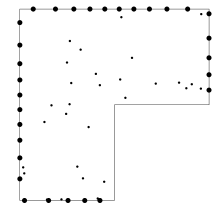
Figure 1. The L-shaped region with points on the boundary as well as random points the interior.

Solutions of $\Delta u+\lambda u=0$ in the plane are found by the method of separation of variables: if $u=f(r)g(\theta)$ in polar coordinates, then

$$r^{2}\frac{\Delta u}{u}=\frac{g^{\prime\prime}(\theta)}{g(\theta)}+r^{2}\frac{f^{\prime\prime}(r)}{f(r)}+r\frac{f^{\prime}(r)}{f(r)},$$

so that the equation $\Delta u+\lambda u=0$ decouples into

(5) $$g^{\prime\prime}(\theta)+Kg(\theta)=0,\quad r^{2}f^{\prime\prime}(r)+rf^{\prime}(r)+(\lambda r^{2}-K)f(r)=0$$

for an arbitrary constant $K$. The L-shaped domain has an angle $3\pi/2$ at its reentrant corner, set at the origin. The boundary conditions can be chosen so that the solutions are identically equal to zero on the adjacent line segments and also finite at the origin. Then, the first condition forces $K=4k^{2}/9$ with $k\in\mathbb{Z}$. The second equation of Eq. (5) is a variant of Bessel’s equation [39, Eq. 10.2.1], and therefore the solutions that are also finite at the origin are given by

$$g(\theta)=\sin(2k\theta/3),\quad f(r)=J_{2k/3}(\sqrt{\lambda}r),$$

where $J_{2k/3}$ is the Bessel function of the first kind and $k\in\mathbb{N}$. With this basis, the linear combination

(6) $$u(r,\theta)=\sum_{k=1}^{N}c_{k}u_{k}(r,\theta),\qquad\text{with}\quad u_{k}(r,\theta)=\sin(2k\theta/3)J_{2k/3}(\sqrt{\lambda}r)$$

only has to be minimized on the remaining four boundary segments.

2.5.1. Computation of a candidate

With the notation of Section 1, we take $m_{i}=32$ random points in the interior of the domain and $m_{b}=32$ points on the boundary skipping the sides next to the reentrant corner, as shown in Figure 1. For values of $\lambda$ in the interval $[0,20]$, the functions $u_{k}$ from Equation (6) are evaluated at those points and the smallest singular value $\sigma(\lambda)$ of the top part of the $QR$ factorization is computed. The resulting graph when using $N=16$ terms of the expansion is shown in Figure 2(a). In the graph one can see the three minima corresponding to the first three eigenvalues.

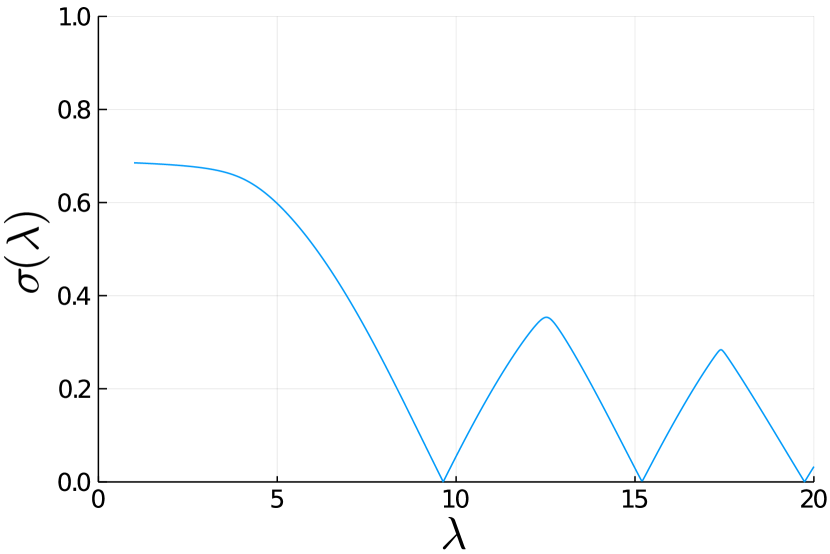
(a) The function $\sigma(\lambda)$.

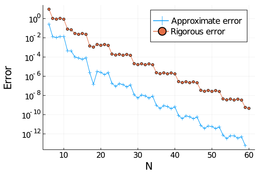
(b) Convergence towards the fundamental eigenvalue.

Figure 2. Results for the L-shaped domain.

2.5.2. Upper bound on the boundary

The upper bound on the boundary is computed as described in Section 2.1, using truncated Taylor expansions with certified bounds on the remainders.

2.5.3. Lower bounding the norm

We lower bound the norm of $u$ by considering the disk sector $G$ with radius 1 and angle $3\pi/2$ inscribed in the domain:

$$\|u\|^{2}=\int_{\Omega}{u^{2}\,dx}\geq\int_{G}u^{2}dx=\int_{0}^{3\pi/2}\int_{0}^{1}ru(r,\theta)^{2}drd\theta.$$

When $u$ is given as a linear expansion of the form (6), orthogonality of the family $\sin(2k\theta/3)$ on the interval $[0,3\pi/2]$ simplifies this last integral to

$$\|u\|^{2} \geq\sum_{k=1}^{N}c_{k}^{2}\int_{0}^{3\pi/2}{\!\!\!\sin(2k\theta/3)^{2}d\theta}\int_{0}^{1}{rJ_{2k/3}(\sqrt{\lambda}r)^{2}dr}$$

$$=\frac{3\pi}{4}\sum_{k=1}^{N}c_{k}^{2}\int_{0}^{1}{rJ_{2k/3}(\sqrt{\lambda}r)^{2}dr}.$$

The remaining integrals $\int_{0}^{1}rJ_{2k/3}(\sqrt{\lambda}r)^{2}dr$ can now be efficiently computed with a certified integrator, giving a lower bound for the norm. In practice we compute the integral from $\epsilon$ to 1 for a small $\epsilon$ to avoid having to deal with the branch cut at 0.

2.5.4. Convergence

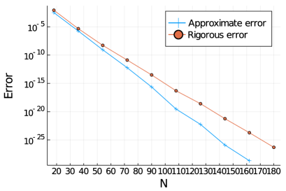
Figure 3. High precision results for convergence towards the fundamental eigenvalue for the L-shaped domain.

The convergence towards the first minimum — the fundamental eigenvalue —  is shown in Figure 2(b). It shows two kinds of convergence. The first one is the approximate error computed as the difference to the “exact” solution obtained with $N=60$. The other one is the radius of the certified enclosure, giving an upper bound on the distance to the exact eigenvalue. While the approximate error wobbles, the certified error is much more stable. We also note that the quotient between the approximate and the certified error remains mostly constant, the precision “lost” when going from the approximate error to the certified error is about 3-4 digits for all $N$ greater than 25. This means that as we compute more and more digits, the relative cost of considering the certified enclosure instead of the approximate error decreases. For $N=60$ we get the enclosure $\lambda\in[9.639723844\pm 4.76\,10^{-10}]$.

As Betcke and Trefethen note, the problem of determining the coefficients $c_{k}$ is highly ill-conditioned. For $N=60$ the condition number of $R(\lambda)$ in Eq. (3) is about $10^{37}$. The values of $A(\lambda)c$ can differ significantly from $Q(\lambda)\tilde{v}$ but are in general still small. This ill-conditioning is not a problem for the computation of the enclosure, since it is not important that we have the “correct” solution, only that the computed solution is small on the boundary.

Since the computations are done with arbitrary precision arithmetic we can go further and compute more digits. Figure 3 shows the convergence for $N$ up to 180. To avoid having to compute the enclosure many times we increase $N$ in steps of 18; other than that the method is the same as in Figure 2(b). These computations take longer: 58 minutes, of which 48% of the time is spent computing the enclosure and the rest on finding the minimum of $\sigma(\lambda)$. The final certified enclosure is

$$\lambda\in[9.63972384402194105271145926\pm 7.36\,10^{-27}].$$

3. Laplace-Beltrami Operators on Spherical Triangles

We now follow the same steps as for the L-shaped region for the Laplace-Beltrami operator on the sphere.

3.1. Laplace-Beltrami Operator on the Sphere

In $\mathbb{R}^{d}$, the Laplacian can be written

$$\Delta=r^{1-d}\frac{\partial}{\partial r}r^{d-1}\frac{\partial}{\partial r}+r^{-2}\Delta_{\mathbb{S}^{d-1}},$$

where $\Delta_{\mathbb{S}^{d-1}}$ is the Laplace-Beltrami operator on the $d$-dimensional sphere. In dimension $d=3$ and spherical coordinates, with $\theta$ denoting the polar angle and $\phi$ the azimuthal angle, it becomes

$$\Delta_{\mathbb{S}^{2}}f(\theta,\phi)=\frac{1}{\sin\theta}\frac{\partial}{\partial\theta}\!\left(\sin\theta\frac{\partial f}{\partial\theta}\right)+\frac{1}{\sin^{2}\theta}\frac{\partial^{2}f}{\partial\phi^{2}}.$$

This is the operator whose fundamental eigenvalue on spherical triangles is of interest for the asymptotics of lattice walks.

3.2. Basis of Solutions

It is classical that separation of variables applies: if $u(\theta,\phi)=f(\theta)g(\phi)$, then

$$\sin^{2}(\theta)\frac{\Delta_{\mathbb{S}^{d-1}}u}{u}=\frac{g^{\prime\prime}(\phi)}{g(\phi)}+\sin^{2}(\theta)\frac{f^{\prime\prime}(\theta)}{f(\theta)}+\sin\theta\cos\theta\frac{f^{\prime}(\theta)}{f(\theta)}.$$

Thus the equation $\Delta_{\mathbb{S}^{d-1}}u+\lambda u=0$ decouples into

(7) $$g^{\prime\prime}(\phi)+Kg(\phi)=0,\quad(1-x^{2})f^{\prime\prime}(x)-2xf^{\prime}(x)+\left(\lambda-\frac{K}{1-x^{2}}\right)f(x)=0,$$

where $\cos\theta=x$, for an arbitrary constant $K$. This is the analogue of Equation (5) in the previous section.

Let $D$ be a spherical triangle. Choose one vertex to place at the north pole. Fix one of the sides on the meridian $\phi=0$ and the other one on the meridian $\phi=\pi/\alpha$. Selecting solutions that are identically 0 on both these meridians fixes $K=\alpha^{2}k^{2}$ with $k\in\mathbb{Z}$. The second equation in Eq. (7) is the associated Legendre equation [39, Eq. 14.2.2]. Its solutions that are real on the interval $(-1,1)$ and finite at $x=1$ (corresponding to the north pole) are the Ferrers functions of the first kind $\mathsf{P}^{\mu}_{\nu}(x)$ with $\mu=-\alpha k$, $k\in\mathbb{N}$ and $\nu$ obeying $\lambda=\nu(\nu+1)$ [39, Eq. 14.8.1]. Thus we are looking for coefficients $c_{k}$ such that the sum

(8) $$u(\theta,\phi)=\sum_{k=1}^{N}{c_{k}\sin(k\alpha\phi)\mathsf{P}^{-k\alpha}_{\nu}(\cos\theta)},\qquad\text{where}\quad\nu(\nu+1)=\lambda$$

vanishes numerically on the opposite side of the triangle. This is the analogue of Equation (6) in the previous section.

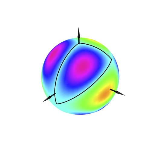
Figure 4. Approximate eigenfunction from Eq. (8) for the fundamental eigenvalue on the spherical triangle $T_{2}$, with angles $2\pi/3$ (at the north pole), $\pi/3$ (on the meridian $\phi=0$) and $\pi/2$. The function is defined except at the south pole and satisfies $\Delta u+\lambda u=0$ in that domain; it is numerically 0 on the boundary of $T_{2}$. The values of the function are represented by colors. The triangle is drawn in black.

3.3. Upper bound on the maximum

By design, $u$ is identically zero on two sides of the triangle and it is sufficient to bound the maximum on the third side. From the differential equation (7) one can obtain a recurrence for the Taylor coefficients of the Ferrers functions. This allows us to compute Taylor expansions of $u$ when bounding the maximum. In the computations we use Taylor expansions of the same order as the number of terms in $u$.

3.4. Lower bound on the norm

We compute the norm on the subset of $D$ which in spherical coordinates is given by the rectangle

$$G=\{(\theta,\phi)\in\mathbb{S}^{2}:0\leq\phi\leq\pi/\alpha,\ 0\leq\theta\leq\beta\},$$

where $\beta$ is the minimum value of $\theta$ on the lower boundary of the triangle. The rectangle $G$ is equal to $D$ precisely when the two angles not at the north pole are both equal to $\pi/2$. The lower bound is obtained from

$$\|u\|_{2}=\int_{D}u^{2}\,dx\geq\int_{G}u^{2}\,dx=\int_{0}^{\pi/\alpha}\int_{0}^{\beta}u(\theta,\phi)^{2}\sin(\theta)d\theta d\phi.$$

As in the plane, when $u$ is of the form given by Equation (8) the orthogonality of the family $\sin(k\alpha\phi)$ on the interval $[0,\pi/\alpha]$ simplifies this integral to

$$\|u\|_{2}\geq\frac{\pi}{2\alpha}\sum_{k=1}^{N}c_{k}^{2}\int_{0}^{\beta}\mathsf{P}^{-k\alpha}_{\nu}(\cos\theta)^{2}\sin\theta\,d\theta.$$

The integrals $\int_{0}^{\beta}\mathsf{P}^{-k\alpha}_{\nu}(\cos\theta)^{2}\sin\theta\,d\theta$ can now be efficiently computed with a certified integrator, giving us a lower bound for the norm. In practice we compute the integral from $\epsilon$ to $\beta$ for a small $\epsilon$ to avoid having to deal with the branch cut at 0, while not losing too much precision on the bound.

3.5. Certification of the index

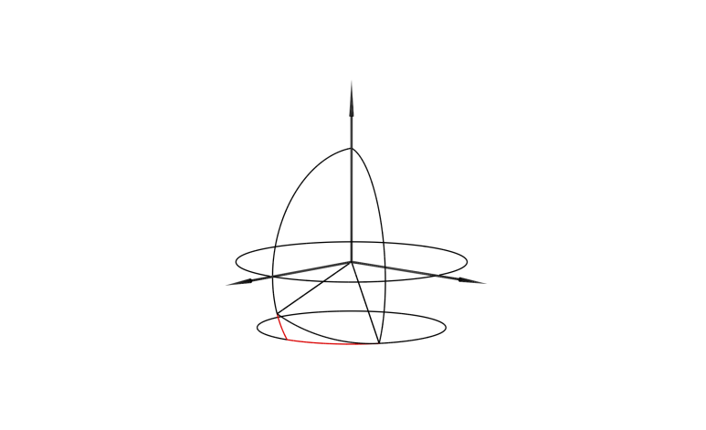
Figure 5. Enclosing sector of a spherical cap (in red) for the spherical triangle $T_{2}$ (in black), with angles $\pi/3$ (at the north pole), $2\pi/3$ (on the meridian $\phi=0$) and $\pi/2$.

That the computed eigenvalue is the fundamental one is certified by showing that the second eigenvalue of the Laplacian on a larger domain is larger than it. This implies that this computed eigenvalue is smaller than the second one and thus has to be the first one.

We consider the domain given by a sector of a spherical cap with its vertex at the north pole and polar angle $\theta_{T}$ equal to the maximal polar angle of the points in the original triangle (see Figure 5.) The corresponding eigenfunctions are the products $\sin(k\alpha\phi)\mathsf{P}_{\nu}^{-k\alpha}(\cos\theta)$ such that $\mathsf{P}_{\nu}^{-k\alpha}(\cos\theta_{T})=0$, with corresponding eigenvalue $\lambda=\nu(\nu+1)$ (see Equation (8)). Thus we want to find the second one in the infinite set of zeros in $\nu$ of the set of Ferrers functions $\{\mathsf{P}_{\nu}^{-k\alpha}(\cos\theta_{T})\mid k\in\mathbb{N}\setminus\{0\}\}$. The study of this infinite set of zeroes is simplified by the following.

Lemma 1.

Assume $x_{0}\in(-1,1)$ is the largest zero of $\mathsf{P}^{\mu}_{\nu}(x)$ (with $\mu\leq 0$), then for any $(\tilde{\mu},\tilde{\nu})$ such that $\tilde{\mu}<\mu$ and $\tilde{\nu}\leq\nu$, the function $\mathsf{P}^{\tilde{\mu}}_{\tilde{\nu}}(x)$ does not vanish in the interval $[x_{0},1)$.

Thus, denoting by $\zeta_{k,j}$ the $j$th zero of $\mathsf{P}^{-k\alpha}_{\nu}(\cos\theta_{T})$ as a function of $\nu$, if a triangle has computed eigenvalue $\lambda=\nu(\nu+1)$, it is sufficient to show that $\zeta_{1,2}$ and $\zeta_{2,1}$ are both larger than $\nu$ to certify that $\lambda$ is indeed the fundamental eigenvalue.

Proof of the lemma.

The basic idea is to use Sturm’s comparison theorem in order to show that the largest zero $\tilde{x}_{0}$ of $\mathsf{P}^{\tilde{\mu}}_{\tilde{\nu}}(x)$ in $(-1,1)$ satisfies $\tilde{x}_{0}<x_{0}$.

The associated Legendre equation (7) can be rewritten

$$((1-x^{2})w^{\prime})^{\prime}+q_{\mu,\nu}(x)w=0,\qquad\text{with}\quad q_{\mu,\nu}(x)=\nu(\nu+1)-\frac{\mu^{2}}{1-x^{2}}$$

and the inequality $q_{\tilde{\mu},\tilde{\nu}}(x)<q_{\mu,\nu}(x)$ for $x\in(-1,1)$ follows from the hypotheses. The proof is by contradiction. Assume $\mathsf{P}^{\mu}_{\nu}$ does not vanish in $[\tilde{x}_{0},1)$. For simplicity of notation, write $w=\mathsf{P}^{\mu}_{\nu}$ and $\tilde{w}=\mathsf{P}^{\tilde{\mu}}_{\tilde{\nu}}$. Then a direct verification shows Picone’s identity

$$\left((1-x^{2})\frac{\tilde{w}}{w}(\tilde{w}^{\prime}w-w^{\prime}\tilde{w})\right)^{\prime}=\\ (q_{\mu,\nu}-q_{\tilde{\mu},\tilde{\nu}})\tilde{w}^{2}+(1-x^{2})\left(\tilde{w}^{\prime}-w^{\prime}\frac{\tilde{w}}{w}\right)^{2},$$

whose right-hand side is positive in $[\tilde{x}_{0},1)$. This implies that the function

$$(1-x^{2})\frac{\tilde{w}}{w}(\tilde{w}^{\prime}w-w^{\prime}\tilde{w})$$

is increasing in that interval. However, it is 0 at $\tilde{x}_{0}$ while as $x\rightarrow 1-$, it behaves like

$$(\tilde{\mu}-\mu)2^{\tilde{\mu}}(1-x)^{-\tilde{\mu}}$$

and thus tends to 0 at $1$, a contradiction. ∎

Using standard interval methods we can isolate all the roots of the first and second Ferrers functions in the interval $[0,\nu]$ and if there is exactly one root then we are sure that the second ones, $\zeta_{1,2}$ and $\zeta_{2,1}$ are larger than $\nu$ and therefore that $\lambda$ is the fundamental eigenvalue.

The method can fail in case either of $\zeta_{1,2}$ and $\zeta_{2,1}$ is less than $\nu$. In that case, we cannot conclude anything about the index of $\lambda$. One option then is to try a different orientation of the triangle. Depending on which angle of the spherical triangle is placed at the north pole, we get a different set of Ferrers functions to consider. In several of the examples below the method fails with the original orientation but there is always at least one orientation in which it succeeds.

The same approach can be used to find the spherical cap with fundamental eigenvalue $\lambda$, required for the Faber-Krahn inequality in Equation (4). For a spherical cap, the eigenfunctions are $\sin(m\phi)\mathsf{P}_{\nu}^{m}(\cos\theta)$, with $m\in\mathbb{Z}$ for it to be continuous on the whole cap, and with $\mathsf{P}_{\nu}^{m}(\cos\theta)=0$ along the boundary of the cap. The corresponding eigenvalue is $\nu(\nu+1)$. The polar angle of the cap with fundamental eigenvalue $\lambda$ is thus determined by finding the largest zero $x_{0}\in(-1,1)$ of $\mathsf{P}^{m}_{\nu}(x)$ with $\lambda=\nu(\nu+1)$ and $m\in\mathbb{Z}$. Lemma 1 reduces the computation to the case $m=0$, a Legendre function. The area of the cap is then given by $2\pi(1-x_{0})$ and during the computation of the norm, as described in Section 2.2, any region of area larger than this will need to be split.

3.6. Regular triangles

We now present the results obtained by this method for the triangles appearing in Table 3 in the work of Bogosel et al. [12] which have at most one singular vertex, i.e., a vertex whose angle is not of the form $\pi/k$ for some integer $k$, and for which the eigenvalue is not exactly known. These triangles are given in Table 1, together with their computed eigenvalues.

We start by showing the successive steps of the method for the triangle $T_{2}$ with angles $(2\pi/3,\pi/3,\pi/2)$ (see Figure 4).

	Number in [12]	Angles	Eigenvalue	Eigenvalue in [12]
$T_{1}$	8	$\left(\frac{3\pi}{4},\frac{\pi}{3},\frac{\pi}{2}\right)$	12.400051652843377905	12.400051
$T_{2}$	9	$\left(\frac{2\pi}{3},\frac{\pi}{3},\frac{\pi}{2}\right)$	13.744355213213231835	13.744355
$T_{3}$	11	$\left(\frac{2\pi}{3},\frac{\pi}{4},\frac{\pi}{2}\right)$	20.571973537984730557	20.571973
$T_{4}$	12	$\left(\frac{2\pi}{3},\frac{\pi}{3},\frac{\pi}{3}\right)$	21.309407630190445259	21.309407
$T_{5}$	13	$\left(\frac{3\pi}{4},\frac{\pi}{4},\frac{\pi}{3}\right)$	24.456913796299111694	24.456913
$T_{6}$	16	$\left(\frac{2\pi}{3},\frac{\pi}{4},\frac{\pi}{4}\right)$	49.109945263284609920	49.109945

Table 1. Triangles with at most one singular vertex from Table 3 in [12]. Certified, correctly rounded, 20 digit eigenvalues are given. Previously computed eigenvalues are also shown. See Table 3 for more digits.

The value of $\sigma(\lambda)$ is given in Figure 6(a). It was generated using an expansion at the singular vertex, with 8 terms, using 16 random points in the interior and 16 points on the boundary opposite to the singular vertex. The plot shows 4 minima, the first of which we need to certify as corresponding to the fundamental eigenvalue.

The convergence towards the first minimum is shown in Figure 6(b). Similarly to Figure 2(b), it shows two kinds of convergence, the approximate error computed as the difference to the “exact” solution obtained with $N=48$ and the certified enclosure. The quotient between the approximate and the certified error increases slightly with $N$, the precision “lost” when going from the approximate error to the certified error is slightly more than 5 digits. For $N=48$ we get the enclosure $\lambda\in[13.7443552132132318354011\pm 3.11\,10^{-23}]$. See Table 3 for more digits.

With the vertex with angle $2\pi/3$ placed at the north pole we get the zeros $\zeta_{1,2}\in[3.6550969\pm 4.82\,10^{-8}]$ and $\zeta_{2,1}\in[3.4315893\pm 5.43,10^{-8}]$ for the enclosing spherical cap sector. Since $\lambda<\zeta_{1,2}(\zeta_{1,2}+1)$ and $\lambda<\zeta_{2,1}(\zeta_{2,1}+1)$ it is smaller than the second eigenvalue of the enclosing spherical cap sector and must therefore correspond to the fundamental eigenvalue of the triangle.

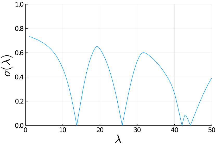
(a) The function $\sigma(\lambda)$.

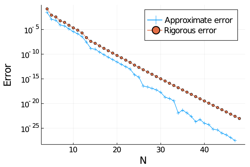
(b) Convergence to the eigenvalue corresponding to the first minimum of $\sigma(\lambda)$.

Figure 6. Results for the triangle $T_{2}$ from Table 1

For the other triangles in Table 1, the method is the same except for the triangles $T_{4}$ and $T_{6}$. For these triangles the two non-singular angles are the same. This symmetry in the domain implies a corresponding symmetry for the eigenfunction. The approximate solution can be forced to have the same symmetry by using only every second term from the sum in Equation (8), which improves the convergence rate. Figure 7 shows the convergence for the radius of the enclosures. The rate of convergence varies between the triangles, the best convergence being obtained for the triangles $T_{4}$ and $T_{6}$ where the mentioned symmetry was used. Even though they converge at different rates they all show linear convergence. As in the case of the L-shaped domain the condition number of $R(\lambda)$ is huge for all of them, $T_{6}$ has the highest value at $10^{300}$. As in the previous cases the solutions is however still small on the boundary.

For all these triangles we are also able to certify that the computed eigenvalue indeed corresponds to the fundamental eigenvalue by lower bounding the second eigenvalue of the enclosing circular cap sector.

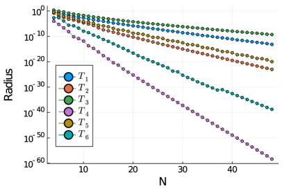
Figure 7. Convergence of the enclosure for the six triangles in Table 1.

High precision results

We give high precision computations of the same eigenvalues in Figure 8(a). Compared to Figure 7 we start the computations at $N=16$ and increase $N$ by 16 at a time. Figure 8(b) shows the time taken for both computing the minimum of $\sigma(\lambda)$ and computing the enclosure for different triangles as $N$ varies. This shows that for large values of $N$ the cost of certifying the enclosure is a relatively small part of the computation, and in particular, the time for bounding the norm accounts for only a few seconds of the total time. Correctly rounded eigenvalues are given in Table 3.

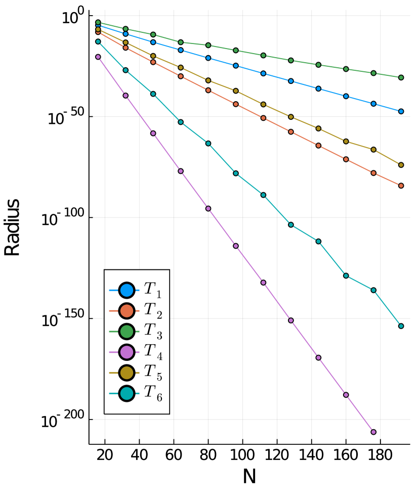
(a) High precision computations of the enclosure

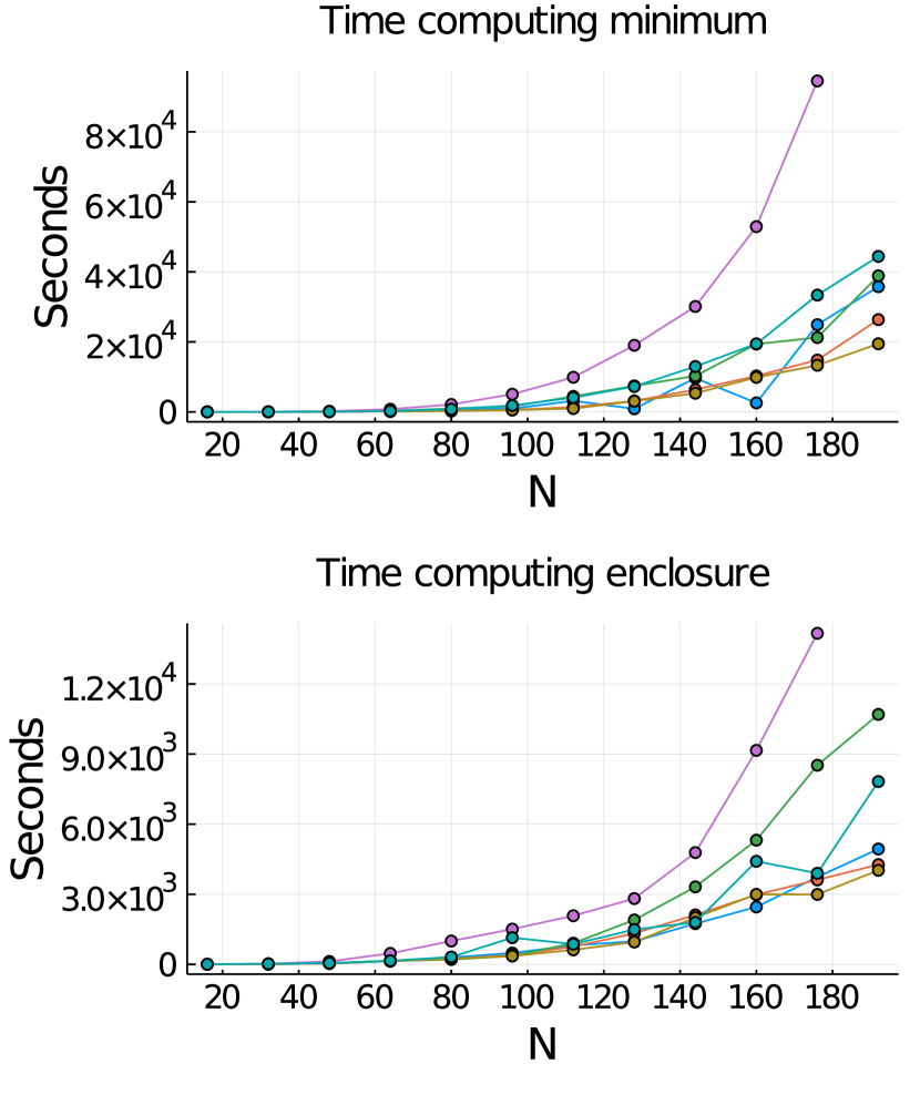
(b) Time for computing the minimum of $\sigma(\lambda)$ as well as the enclosure.

Figure 8. High precision computations for the triangles in Table 1.

3.7. Singular triangles

As shown above, the method of particular solutions works well for the triangles in Table 1, using an expansion at the single singular vertex. This is not sufficient for the singular triangles listed in Table 2. Those are the triangles from Table 3 in [12] with more than one singular vertex.

	Number in [12]	Angles	Eigenvalue	Eigenvalue in [12]
$T_{7}$	1	$\left(\frac{2\pi}{3},\frac{3\pi}{4},\frac{3\pi}{4}\right)$	4.2617347552939870857	4.261734
$T_{8}$	2	$\left(\frac{2\pi}{3},\frac{2\pi}{3},\frac{2\pi}{3}\right)$	5.1591456424665417112	5.159145
$T_{9}$	3	$\left(\frac{\pi}{2},\frac{2\pi}{3},\frac{3\pi}{4}\right)$	6.2417483307263342368	6.241748
$T_{10}$	4	$\left(\frac{\pi}{2},\frac{2\pi}{3},\frac{2\pi}{3}\right)$	6.7771080545983009574	6.777108

Table 2. Triangles with more than one singular vertex from Table 3 in [12]. Certified, correctly rounded, 20 digit eigenvalues are given. See Table 3 for more digits.

For such singular cases, a solution suggested by Betcke and Trefethen is to use expansions at all singular vertices. For a spherical triangle where all of the vertices are singular our candidate eigenfunction will be of the form

$$u(\theta,\phi)=u_{1}(\theta_{1},\phi_{1})+u_{2}(\theta_{2},\phi_{2})+u_{3}(\theta_{3},\phi_{3})$$

with

$$u_{i}(\theta,\phi)=\sum_{k=1}^{N_{i}}c_{i,k}\sin(k\alpha_{i}\phi)\mathsf{P}^{-k\alpha_{i}}_{\nu}(\cos\theta)$$

and $(\theta_{i},\phi_{i})$ corresponds to $(\theta,\phi)$ in spherical coordinates with vertex $i$ on the north pole. This method does not work well in our cases. Triangle $T_{9}$ from Table 2 has two singular vertices. Using expansions with 8 terms at each one gives the plot of $\sigma(\lambda)$ seen in Figure 9(a). This plot is less smooth than the corresponding one for the regular triangle (Figure 6(a)). As the number of terms is increased the picture does not improve. Convergence of the first minimum is show in Figure 9(b) where there error is computed by comparing it to $\lambda=6.24174833072633424$. Increasing the number of terms past 26 does not improve the approximation.

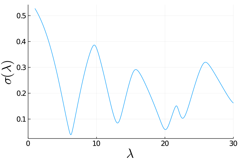
(a) The function $\sigma(\lambda)$ with $N=16$ terms.

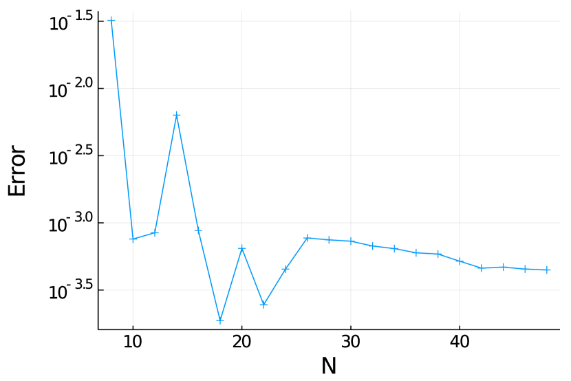
(b) Convergence of the first minimum. No improvement is seen as the number of terms is increased past 26.

Figure 9. Results for the triangle $T_{9}$ from Table 2 using expansions with $N/2$ terms at each of the two singular vertices.

A solution we found to work satisfactorily is to complement the above approach with an expansion at an interior point. For a triangle with three singular vertices this gives us the candidate

$$u(\theta,\phi)=u_{1}(\theta_{1},\phi_{1})+u_{2}(\theta_{2},\phi_{2})+u_{3}(\theta_{3},\phi_{3})+u_{\text{int}}(\theta_{\text{int}},\phi_{\text{int}})$$

where $(\theta_{\text{int}},\phi_{\text{int}})$ is given in spherical coordinates with the interior point placed at the north pole and $u_{\text{int}}$ contains $N_{\text{int}}$ terms and is of the form

$$u_{\text{int}}(\theta,\phi)= c_{\text{int},1}\mathsf{P}_{\nu}^{0}(\cos(\theta))+c_{\text{int},2}\sin(\phi)\mathsf{P}_{\nu}^{1}(\cos(\theta))+c_{\text{int},3}\cos(\phi)\mathsf{P}_{\nu}^{1}(\cos(\theta))$$

$$+c_{\text{int},4}\sin(2\phi)\mathsf{P}_{\nu}^{2}(\cos(\theta))+c_{\text{int},5}\cos(2\phi)\mathsf{P}_{\nu}^{2}(\cos(\theta))+\cdots.$$

Using this expansion for triangle $T_{9}$ with the interior point chosen to be the center of the triangle, given by the sum of the vertices normalized to be on the sphere, and 3 terms from the two singular vertices combined with 12 terms from the interior gives the plot of $\sigma(\lambda)$ seen in Figure 10(a). Compared to Figure 9(a) the minima are more distinct. The convergence towards the first minimum is shown in Figure 10(b). Like Figure 6(b) it shows both the approximate error and the radius of the computed enclosure. Even though there are more oscillations than for the regular triangles, we see convergence as $N$ is increased. For $N=48$ we get the enclosure $\lambda\in[6.24175\pm 8.42\,10^{-6}]$. We have used the same number of terms for each of the two singular vertices and four times that number of terms for the interior point. The upper bound of the maximum on the boundary is computed in the same way as for the regular triangles except that it is no longer identically equal to zero on two of the boundaries. For the lower bound of the norm, the terms in the expansion are no longer orthogonal and we have to resort to the second method described in Section 2.2. Since the first eigenfunction has constant sign and is very smooth we do not need a very fine partitioning to get a good lower bound. The interior domain $\Omega^{\prime}$ we use is the triangle with vertices given by the points in the middle between the center and the vertices of the original triangle. Partitioning $\Omega^{\prime}$ into four separate triangles yields a sufficiently good lower bound. Still the computation of the norm is much more costly than in the case of regular triangles.

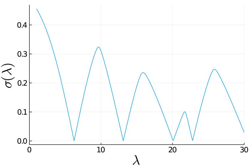
(a) The function $\sigma(\lambda)$ using expansions with 3 terms at each vertex as well as 12 interior terms.

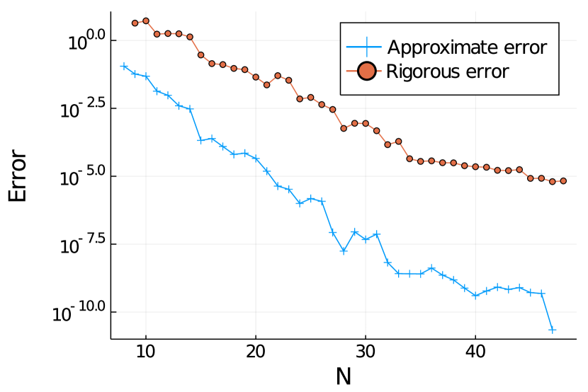
(b) Convergence towards the eigenvalue corresponding to the first minimum for triangle $T_{9}$ from Table 2.

Figure 10. Results for the triangle $T_{9}$ from Table 2. .

Figure 11 shows the convergence for all the triangles in Table 2. Again there are more oscillations than for the regular triangles but still convergence as the number of terms is increased. The triangles $T_{7}$, $T_{8}$ and $T_{10}$ all have symmetries that have been used to improve the convergence. For $T_{7}$ only every second term occurs in the expansion for both $u_{1}$ and $u_{\text{int}}$. In $T_{8}$ we take only every second term from $u_{1}$, $u_{2}$ and $u_{3}$. Finally for $T_{10}$ every second term is used in $u_{\text{int}}$. In several cases, there is potential to make more use of symmetries; for $T_{8}$, this is done in Section 3.9. As in the previous examples $A(\lambda)$ is ill-conditioned, though slightly less so than before, with condition number varying between $10^{19}$ and $10^{51}$ for the four triangles. Again, the solution is still small on the boundary and we get good enclosures.

As in the case of regular triangles, we are also able to certify that the computed eigenvalue indeed corresponds to the fundamental eigenvalue by lower bounding the eigenvalue of the enclosing circular cap sector.

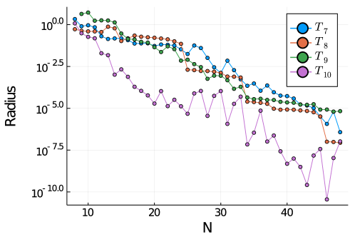
Figure 11. Convergence of the enclosure for the four triangles in Table 2.

High precision results for the same triangles are presented in Figure 12(a) and timings in Figure 12(b). The situation is very similar to that of the regular triangles in Figure 8(a) and 8(b) except that the rate of convergence is lower. The computation of the norm takes up a larger part of the time than for the regular triangles but is still dominated by the computation of the minimum for high values of $N$.

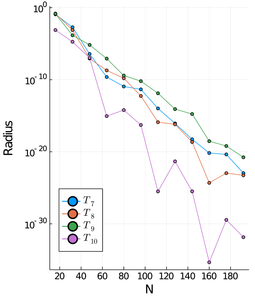
(a) High precision computations of the enclosure

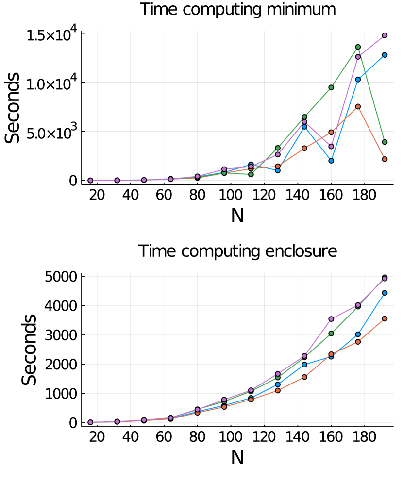
(b) Time for computing the minimum of $\sigma(\lambda)$ as well as the enclosure.

Figure 12. High precision computations for the triangles in Table 2.

3.8. Combinatorial application: denominators of asymptotic exponents

Our motivation in this study is to obtain lower bounds on the denominators the asymptotic exponents $\alpha$ in Equation (1) would have if they were rational numbers.

This is achieved by the computation of a continued fraction expansion, a routine technique in experimental mathematics. First, the exponent $\alpha$ is computed using interval arithmetic from the enclosure of the fundamental eigenvalue. Next, the regular continued fraction is computed using interval arithmetic and the computation is stopped at the first time a partial quotient cannot be guaranteed. The sequence of integers thus obtained is used to compute exactly the first convergents $(P_{n}/Q_{n})$ of the continued fraction. Unless the number is thus detected to be rational, the last $Q_{n}$ is a lower bound on the actual denominator. The computed lower bounds are listed in Table 4 in the Appendix.

3.9. 3D Kreweras walks

In dimension 2, the Kreweras walks are walks with step set $\{(-1,0),(0,-1),(1,1)\}$ whose study started with a 100-page article by Kreweras [30] showing in particular that the generating functions of interest are algebraic (and therefore solutions of a linear differential equation), but the proof is far from trivial. In dimension 2, all step sets with small steps (where each coordinate has absolute value at most 1) having generating functions that are solutions of a linear differential equation are also step sets for which an associated group of the walk is finite [14]. This is just an observation obtained by looking at all possible cases. It is natural to wonder whether a deeper relation between this group and the generating functions could explain this property.

In dimension 3, the 3D Kreweras walks are defined as the natural generalization of the 2D case, with step set $\{(-1,0,0),(0,-1,0),(0,0,-1),(1,1,1)\}$, for which the analogous group is again finite. That step set leads to the study of the spherical triangle with angles $(2\pi/3,2\pi/3,2\pi/3)$ and its fundamental eigenvalue [12]. The history of the knowledge on this eigenvalue, following Bogosel et al. [12] and a private communication of Bostan, is as follows:

• $[5.15,5.16]$ in 2008 by Costabel (unpublished?);

• 5.158968860560663 in 2009 by Ratzkin and Treibergs [42];

• 5.1606 in 2013 by Balakrishna [3];

• 5.159145642466 in 2015 by Guttmann (unpublished);

• 5.1591452 in 2016 by Bacher, Kauers and Yatchak [2];

• 5.159145642470 in 2020 by Bogosel, Perrollaz, Raschel and Trotignon [12].

We can now certify that the eigenvalue is actually

$$\lambda=5.1591456424665417112216748625993501893151700566462081663\\ 0858031086922413365742186774243415327168103656498\dots{}$$

The corresponding exponent $\alpha=-1-\sqrt{\lambda+1/4}$ is

$$\alpha=-3.325757004174456250974540734758388852786843862030738206\\ 09206024964659686065647234082158565813950933996592\dots{}$$

with continued fraction

$$[-4;1,2,14,3,100,12,102,1,5,1,2,7,6,1,11,1,6,4,1,\\ 8,3,3,1,1,44,8,3,1,3,5,1,1,2,1,2,1,4,1,1,1,6,\\ 4,1,2,1,3,2,1,15,1,17,1,2,1,2,1,1,5,1,2,2,13,1,\\ 3,15,2,1,2,1,6,6,2,1,1,1,1,2,3,1,1,19,5,1,4,2,\\ 7,1,1,5,1,23,195,1,1,3,1,1,3,1,1,1,1,1,9,2,\dots].$$

This implies that if it is a rational number, its denominator must be at least

$$9571644798056984399060418592860369800792627450626933>10^{51}.$$

The computation to high accuracy exploits the symmetry of the triangle. We use expansions at all vertices together with one from the interior, but compared to Section 3.7 we make full use of the symmetry of the domain. All of the vertices are symmetric and hence we expect the coefficients for their expansions to be the same. In addition, only every second term will appear. For the interior expansion we get a six-fold symmetry and only every sixth term appears. This gives us the expansion

$$u(\theta,\phi)=\sum_{l=1}^{N_{2}}b_{k}\cos(3(l-1)\alpha\phi_{\text{int}})\mathsf{P}_{\nu}^{-3(l-1)\alpha}(\cos(\theta_{\text{int}}))\\ +\sum_{k=1}^{N_{1}}c_{k}\left(\sin((2(k-1)+1)\alpha\phi_{1})\mathsf{P}_{\nu}^{-(2(k-1)+1)\alpha}(\cos(\theta_{1}))\right.\\ \qquad\qquad+\sin((2(k-1)+1)\alpha\phi_{2})\mathsf{P}_{\nu}^{-(2(k-1)+1)\alpha}(\cos(\theta_{2}))\\ +\left.\sin((2(k-1)+1)\alpha\phi_{3})\mathsf{P}_{\nu}^{-(2(k-1)+1)\alpha}(\cos(\theta_{3}))\right).$$

One benefit with our method is that we do not have to prove that the above expansion satisfies the required symmetries, we just see a better convergence if it does. The only property of the expansion that we use when computing the enclosure is that it behaves in the same way on all three boundaries. It is therefore sufficient to bound the maximum on only one of them.

References

- [1] M. S. Ashbaugh and H. A. Levine, Inequalities for the Dirichlet and Neumann eigenvalues of the Laplacian for domains on spheres, in Journées “Équations aux Dérivées Partielles” (Saint-Jean-de-Monts, 1997), École Polytech., Palaiseau, 1997, pp. I–1–I–15.
- [2] A. Bacher, M. Kauers, and R. Yatchak, Continued classification of 3d lattice models in the positive octant, in FPSAC 2016, vol. BC of DMTCS Proceedings, 2016, pp. 95–106.
- [3] B. S. Balakrishna, On multi-particle Brownian survivals and the spherical Laplacian, Tech. Report 44459, Munich Personal RePEc Archive, 2013, https://mpra.ub.uni-muenchen.de/44459/.
- [4] A. H. Barnett and A. Hassell, Boundary quasi-orthogonality and sharp inclusion bounds for large Dirichlet eigenvalues, SIAM J. Numer. Anal., 49 (2011), pp. 1046–1063, https://doi.org/10.1137/100796637.
- [5] H. Behnke and F. Goerisch, Inclusions for eigenvalues of selfadjoint problems, in Topics in validated computations (Oldenburg, 1993), vol. 5 of Stud. Comput. Math., North-Holland, Amsterdam, 1994, pp. 277–322, https://doi.org/10.1016/0021-8502(94)90369-7.
- [6] P. Bérard and G. Besson, Spectres et groupes cristallographiques. II. Domaines sphériques, Ann. Inst. Fourier (Grenoble), 30 (1980), pp. 237–248, http://www.numdam.org/item?id=AIF_1980__30_3_237_0.
- [7] P. H. Bérard, Remarques sur la conjecture de Weyl, Compositio Math., 48 (1983), pp. 35–53, http://www.numdam.org/item?id=CM_1983__48_1_35_0.
- [8] T. Betcke, The generalized singular value decomposition and the method of particular solutions, SIAM J. Sci. Comput., 30 (2008), pp. 1278–1295, https://doi.org/10.1137/060651057.
- [9] T. Betcke and L. N. Trefethen, Reviving the method of particular solutions, SIAM Rev., 47 (2005), pp. 469–491, https://doi.org/10.1137/S0036144503437336.
- [10] J. Bezanson, A. Edelman, S. Karpinski, and V. B. Shah, Julia: A fresh approach to numerical computing, SIAM Review, 59 (2017), pp. 65–98, https://doi.org/10.1137/141000671.
- [11] D. Boffi, Finite element approximation of eigenvalue problems, Acta Numer., 19 (2010), pp. 1–120, https://doi.org/10.1017/S0962492910000012.
- [12] B. Bogosel, V. Perrollaz, K. Raschel, and A. Trotignon, 3d positive lattice walks and spherical triangles, Journal of Combinatorial Theory, Series A, 172 (2020), p. 105189, https://doi.org/10.1016/j.jcta.2019.105189.
- [13] A. Bostan, Computer algebra for lattice path combinatorics, tech. report, 2019.
- [14] A. Bostan, K. Raschel, and B. Salvy, Non-D-finite excursions in the quarter plane, Journal of Combinatorial Theory, Series A, 121 (2014), pp. 45–63, https://doi.org/10.1016/j.jcta.2013.09.005.
- [15] H. Brezis, Functional analysis, Sobolev spaces and partial differential equations, Universitext, Springer, New York, 2011.
- [16] E. Cancès, G. Dusson, Y. Maday, B. Stamm, and M. Vohralík, Guaranteed and robust a posteriori bounds for Laplace eigenvalues and eigenvectors: conforming approximations, SIAM J. Numer. Anal., 55 (2017), pp. 2228–2254, https://doi.org/10.1137/15M1038633.
- [17] R. Courant and D. Hilbert, Methods of mathematical physics, vol. 1, Wiley, 1962.
- [18] D. Denisov and V. Wachtel, Random walks in cones, Ann. Probab., 43 (2015), pp. 992–1044, https://doi.org/10.1214/13-AOP867.
- [19] J. Descloux and M. Tolley, An accurate algorithm for computing the eigenvalues of a polygonal membrane, Comput. Methods Appl. Mech. Engrg., 39 (1983), pp. 37–53, https://doi.org/10.1016/0045-7825(83)90072-5.
- [20] C. Fieker, W. Hart, T. Hofmann, and F. Johansson, Nemo/Hecke: Computer algebra and number theory packages for the Julia programming language, in Proceedings of the 2017 ACM on International Symposium on Symbolic and Algebraic Computation, ISSAC ’17, New York, NY, USA, 2017, ACM, pp. 157–164, https://doi.org/10.1145/3087604.3087611.
- [21] L. Fousse, G. Hanrot, V. Lefèvre, P. Pélissier, and P. Zimmermann, MPFR: A multiple-precision binary floating-point library with correct rounding, ACM Trans. Math. Softw., 33 (2007), p. 13, https://doi.org/10.1145/1236463.1236468.
- [22] L. Fox, P. Henrici, and C. Moler, Approximations and bounds for eigenvalues of elliptic operators, SIAM J. Numer. Anal., 4 (1967), pp. 89–102, https://doi.org/10.1137/0704008.
- [23] J. Gómez-Serrano and G. Orriols, Any three eigenvalues do not determine a triangle, arXiv e-prints, (2019), arXiv:1911.06758, p. arXiv:1911.06758, https://arxiv.org/abs/1911.06758.
- [24] A. Gopal and L. N. Trefethen, Solving Laplace problems with corner singularities via rational functions, SIAM J. Numer. Anal., 57 (2019), pp. 2074–2094, https://doi.org/10.1137/19M125947X.
- [25] D. S. Grebenkov and B.-T. Nguyen, Geometrical structure of Laplacian eigenfunctions, SIAM Rev., 55 (2013), pp. 601–667, https://doi.org/10.1137/120880173.
- [26] F. Johansson, Arb: efficient arbitrary-precision midpoint-radius interval arithmetic, IEEE Trans. Comput., 66 (2017), pp. 1281–1292, https://doi.org/10.1109/TC.2017.2690633.
- [27] F. Johansson and M. Mezzarobba, Fast and rigorous arbitrary-precision computation of Gauss-Legendre quadrature nodes and weights, SIAM J. Sci. Comput., 40 (2018), pp. C726–C747, https://doi.org/10.1137/18M1170133.
- [28] R. S. Jones, Computing ultra-precise eigenvalues of the Laplacian within polygons, Adv. Comput. Math., 43 (2017), pp. 1325–1354, https://doi.org/10.1007/s10444-017-9527-y.
- [29] C. Krattenthaler, Lattice path enumeration, in Handbook of enumerative combinatorics, Discrete Math. Appl. (Boca Raton), CRC Press, Boca Raton, FL, 2015, pp. 589–678.
- [30] G. Kreweras, Sur une classe de problèmes de dénombrement liés au treillis des partitions des entiers, Cahiers du B.U.R.O., 6 (1965), pp. 5–105.
- [31] J. R. Kuttler and V. G. Sigillito, Eigenvalues of the Laplacian in two dimensions, SIAM Rev., 26 (1984), pp. 163–193, https://doi.org/10.1137/1026033.
- [32] X. Liu, A framework of verified eigenvalue bounds for self-adjoint differential operators, Appl. Math. Comput., 267 (2015), pp. 341–355, https://doi.org/10.1016/j.amc.2015.03.048.
- [33] X. Liu and S. Oishi, Verified eigenvalue evaluation for the Laplacian over polygonal domains of arbitrary shape, SIAM J. Numer. Anal., 51 (2013), pp. 1634–1654, https://doi.org/10.1137/120878446.
- [34] K. Makino and M. Berz, Taylor models and other validated functional inclusion methods, International Journal of Pure and Applied Mathematics, 4 (2003), pp. 379–456, http://bt.pa.msu.edu/pub/papers/TMIJPAM03/TMIJPAM03.pdf.
- [35] P. K. Mogensen and A. N. Riseth, Optim: A mathematical optimization package for Julia, Journal of Open Source Software, 3 (2018), p. 615, https://doi.org/10.21105/joss.00615.
- [36] C. B. Moler and L. E. Payne, Bounds for eigenvalues and eigenvectors of symmetric operators, SIAM J. Numer. Anal., 5 (1968), pp. 64–70, https://doi.org/10.1137/0705004.
- [37] M. T. Nakao, M. Plum, and Y. Watanabe, Numerical verification methods and computer-assisted proofs for partial differential equations, vol. 53 of Springer Series in Computational Mathematics, Springer, Singapore, 2019, https://doi.org/10.1007/978-981-13-7669-6.
- [38] M. T. Nakao, N. Yamamoto, and K. Nagatou, Numerical verifications for eigenvalues of second-order elliptic operators, Japan J. Indust. Appl. Math., 16 (1999), pp. 307–320, https://doi.org/10.1007/BF03167360.
- [39] F. W. J. Olver, D. W. Lozier, R. F. Boisvert, and C. W. Clark, eds., NIST Handbook of Mathematical Functions, Cambridge University Press, 2010.
- [40] R. B. Platte and T. A. Driscoll, Computing eigenmodes of elliptic operators using radial basis functions, Comput. Math. Appl., 48 (2004), pp. 561–576, https://doi.org/10.1016/j.camwa.2003.08.007.
- [41] M. Plum, Bounds for eigenvalues of second-order elliptic differential operators, Zeitschrift für angewandte Mathematik und Physik ZAMP, 42 (1991), pp. 848–863, https://doi.org/10.1007/BF00944567.
- [42] J. Ratzkin and A. Treibergs, A capture problem in Brownian motion and eigenvalues of spherical domains, Trans. Amer. Math. Soc., 361 (2009), pp. 391–405, https://doi.org/10.1090/S0002-9947-08-04505-4.
- [43] B. Salvy and P. Zimmermann, Gfun: a Maple package for the manipulation of generating and holonomic functions in one variable, ACM Trans. Math. Softw., 20 (1994), pp. 163–177, https://doi.org/10.1145/178365.178368.
- [44] G. Still, Computable bounds for eigenvalues and eigenfunctions of elliptic differential operators, Numer. Math., 54 (1988), pp. 201–223, https://doi.org/10.1007/BF01396975.
- [45] A. Strohmaier, Computation of eigenvalues, spectral zeta functions and zeta-determinants on hyperbolic surfaces, in Geometric and computational spectral theory, vol. 700 of Contemp. Math., Amer. Math. Soc., Providence, RI, 2017, pp. 177–205, https://doi.org/10.1090/conm/700/14187.
- [46] W. Tucker, Validated numerics, Princeton University Press, Princeton, NJ, 2011.