Indefinite Mean-Field Type Linear-Quadratic Stochastic Optimal Control Problems

Abstract

This paper focuses on indefinite stochastic mean-field linear-quadratic (MF-LQ, for short) optimal control problems, which allow the weighting matrices for state and control in the cost functional to be indefinite. The solvability of stochastic Hamiltonian system and Riccati equations is presented under both positive definite case and indefinite case. The optimal controls in open-loop form and closed-loop form are obtained, respectively. Moreover, the dynamic mean-variance problem can be solved within the framework of the indefinite MF-LQ problem. Other two examples shed light on the theoretical results established.

Key words: Stochastic linear-quadratic problem, Mean-field, Hamiltonian system, Stochastic differential equations, Forward-backward stochastic differential equations, Riccati equations

AMS subject classification: 93E20, 60H10, 49N10

1 Introduction

Historically, researchers have made many contributions to McKean-Vlasov type stochastic differential equation (SDE, for short) ([1, 2, 8, 11, 13, 16, 20]), which can be regarded as a kind of mean-field SDE (MF-SDE, for short). In recent years, stochastic mean-field optimal control problems, mean-field differential games and their applications have attracted researchers’ attention. Andersson and Djehiche [4], and Buckdahn et al. [10] studied the maximum principle for SDEs of mean-field type, respectively. Buckdahn et al. [9] considered the mean-field backward SDE (MF-BSDE), Bensoussan et al. [7] obtained the unique solvability of mean-field type forward-backward SDE (MF-FBSDE). Recently, Duncan and Tembine [14] applied a direct method to discuss an MF-LQ game. Barreiro-Gomez et al. [5] investigated an MF-LQ game of jump-diffusion process with regime switching. This paper focuses on MF-LQ stochastic optimal control problems for the indefinite weighting case, which generalize the work of mean-field type optimal control problems with positive definite weighting case.

For the positive definite case, MF-LQ problems have been studied widely over the past decade. Yong [29] considered an MF-LQ problem with deterministic coefficients over a finite time horizon, and presented the optimal feedback using a system of Riccati equations. Recently, there are some related works following up Yong [29] (see [17, 22, 30, 28, 27]). Different from deterministic LQ problem, in the cost functional, the cost weighting matrices for the state and the control are allowed to be indefinite. We notice that in the stochastic LQ setting, the cost functional with indefinite cost weighting matrices may still be convex in control. It is precisely this feature that determines whether an optimal control exists. Indefinite stochastic LQ theory has been extensively developed and has lots of interesting applications. Chen et al. [12] studied a kind of indefinite LQ problem based on Riccati equation. Rami et al. [3] showed that the solvability of the generalized Riccati equation is sufficient and necessary condition for the well-posedness of the indefinite LQ problem. Subsequent research includes various cases, and refer to [19, 25, 26].

One of the motivations for indefinite MF-LQ problems comes from the mean-variance portfolio selection problem. Markowitz initially proposed and solved the mean-variance problem in the single-period setting in his Novel-Prize winning work [23, 24], which is an important foundation of the development of modern finance. After Markowitz’s pioneering work, the mean-variance model was extended to multi-period/continuous-time portfolio selection. If one wants to solve the mean-variance portfolio selection, she faces to two-objective: One is to minimize the difference between the terminal wealth and its expected value; the other one is to maximize her expected terminal wealth. Since there are two criteria in one cost functional, this stochastic control problem is significantly different from the classic LQ problem. The main reason is due to the variance term

$$\mbox{Var}(X(T))=\mathbb{E}\big{[}X(T)-\mathbb{E}[X(T)]\big{]}^{2}$$

essentially, which involves the nonlinear term of $(\mathbb{E}[X(T)])^{2}$. In general, for nonlinear utility function $U(\cdot)$, there exists an essential difference between $\mathbb{E}[U(X(T))]$ and $U(\mathbb{E}[X(T)])$, which leads to the fundamental difficulty to deal with the latter one by dynamic programming. Li and Zhou [21] embedded this problem into an auxiliary stochastic LQ problem, which actually is one of indefinite LQ problems. In this paper, we re-visit the continuous-time mean-variance problem using the theoretical results of indefinite MF-LQ problems in a direct way (see the example in Section 5.1).

Besides the dynamic mean-variance portfolio selection problem, there are many phenomena in finance and engineering fields which involve indefinite weighting parameters in the integral term as well as the terminal term. Another motivation is inspired by multi-objective optimization problems involving mean value. These problems can be converted into a single-objective problem by putting weights on the different objectives, which essentially are the indefinite mean-field optimization problems. For example, in a moving high-speed train, the controller wants to improve the speed as high as possible. Except for speeding up the train, the controller also wants to improve the resistance to the stochastic disturbance, which means that the state $X(\cdot)$ of train can not deviate too much from the mean value $\mathbb{E}[X(\cdot)]$. Therefore, there is a tradeoff between two objectives: One is to maximize the total speed $\mathbb{E}\int_{0}^{T}|u(t)|^{2}dt$, the other one is to minimize the variance over interval $[0,T]$ measured by $\mathbb{E}\int_{0}^{T}|X(t)-\mathbb{E}[X(t)]|^{2}dt$. We convert this multi-objective optimization problem into a single-objective problem as:

$$J(u(\cdot))=\mathbb{E}\int_{0}^{T}\Big{\{}\alpha\big{|}X(t)-\mathbb{E}[X(t)]\big{|}^{2}-\beta|u(t)|^{2}\Big{\}}dt$$

with $\alpha,\beta>0$. When the system is linear, this problem is a special case of indefinite MF-LQ problem.

In literatures about indefinite LQ problem, the standard matrix inverse is involved in the Riccati equation, requiring the related term to be nonsingular. However, sometimes, the theory of Riccati equation is abstract and difficult. For example, the global solvability of Riccati equation (in the indefinite case or/and in the stochastic case) is often not simple. For this reason, we want to find another element with flexible restrictions instead of Riccati equation. Based on Yong [29] and inspired by Yu [32] and Huang and Yu [18], we generalize the results of positive definite MF-LQ problem to the indefinite case by introducing a relaxed compensator, which can be regarded as a generalization of the solution of Riccati equation. The presence of the relaxed compensator guarantees the well-posedness of MF-LQ problem. The open-loop and closed-loop optimal controls are also obtained under indefinite case. There are three main contributions of this paper:

1. Comparing with the solvability of Riccati equations, the relaxed compensator is defined under more flexible conditions (Condition (RC) in Section 4), which is more general.

2. Based on the linear transformation involving relaxed compensator, we analyze the unique solvability of a kind of MF-FBSDEs, which does not satisfy the monotonicity condition in [7].

3. We obtain the existing of relaxed compensator, which is a sufficient and necessary condition for the solvability of Riccati equations.

Recently, Sun [26] studied the MF-LQ problem under a uniform convexity condition, and showed that the convergence of a family of uniformly convex cost functionals is equivalent to the open-loop solvability of the MF-LQ problem. Different from the method in [26], this paper focuses on how to find a relaxed compensator to extend the condition of cost functional from positive case to the indefinite case.

The rest of this paper is organized as follows. We present some preliminaries and formulate an MF-LQ problem in Section 2. Section 3 is devoted to studying the MF-LQ problem under positive definite case. Section 4 focuses on the indefinite MF-LQ problem, and derives the open-loop optimal control and the optimal feedback control. Section 5 illustrates some applications including the dynamic mean-variance problem and other two examples.

2 Problem formulation and preliminaries

We denote by $\mathbb{R}^{n}$ the $n$-dimensional Euclidean space. Let $\mathbb{R}^{n\times m}$ be the set of all $(n\times m)$ matrices. Let $\mathbb{S}^{n}\subset\mathbb{R}^{n\times n}$ be the collection of all symmetric matrices. As usual, if a matrix $A\in\mathbb{S}^{n}$ is positive semidefinite (resp. positive definite; negative semidefinite; negative definite), we denote $A\geq 0$ (resp. $>0$; $\leq 0$; $<0$). All the positive semidefinite (resp. negative semidefinite) matrices are collected by $\mathbb{S}^{n}_{+}$ (resp. $\mathbb{S}^{n}_{-}$). Let $(\Omega,\mathcal{F},\mathbb{P},\mathbb{F})$ be a complete filtered probability space on which a one-dimensional standard Brownian motion $W(\cdot)$ is defined with $\mathbb{F}\equiv\{\mathcal{F}_{t}\}_{t\geq 0}$ being its natural filtration augmented by all $\mathbb{P}$-null sets. For simplicity, we will restrict ourselves to the case of one-dimensional standard Brownian motion. Some extensions to the case with multi-dimensional standard Brownian motion will be similarly derived examples in Section 5. Let $T>0$ be a finite time horizon. Let $\mathbb{H}=\mathbb{R}^{n}$, $\mathbb{R}^{n\times m}$, $\mathbb{S}^{n}$, $\mathbb{S}^{n}_{+}$, etc. We introduce the following notation which will be used in the paper:

• $L^{\infty}(0,T;\mathbb{H})$ is the space of $\mathbb{H}$-valued continuous functions $\varphi(\cdot)$ such that $\mathop{\mathrm{esssup}}\limits_{t\in[0,T]}|\varphi(t)|<\infty$.

• $C^{1}([0,T];\mathbb{H})$ is the space of $\mathbb{H}$-valued functions $\varphi(\cdot)$ such that $\dot{\varphi}(\cdot)$ is continuous.

• $L^{2}_{\mathcal{F}_{T}}(\Omega;\mathbb{H})$ is the space of $\mathbb{H}$-valued $\mathcal{F}_{T}$-measurable random variables $\xi$ such that $\mathbb{E}[|\xi|^{2}]<\infty$.

• $L^{2}_{\mathbb{F}}(0,T;\mathbb{H})$ is the space of $\mathbb{H}$-valued $\mathbb{F}$-progressively measurable processes $\varphi(\cdot)$ such that $\mathbb{E}\int_{0}^{T}|\varphi(t)|^{2}dt<\infty$.

• $L^{2}_{\mathbb{F}}(\Omega;C([0,T];\mathbb{H}))$ is the space of $\mathbb{H}$-valued $\mathbb{F}$-progressively measurable processes $\varphi(\cdot)$ such that for almost all $\omega\in\Omega$, $r\mapsto\varphi(r,\omega)$ is continuous and $\mathbb{E}\left[\sup\limits_{t\in[0,T]}|\varphi(t)|^{2}\right]<\infty$.

Let $\mathscr{U}[0,T]\equiv L^{2}_{\mathbb{F}}(0,T;\mathbb{R}^{m})$ denote the set of admissible controls. For any initial state $x\in\mathbb{R}^{n}$ and any admissible control $u(\cdot)\in\mathscr{U}[0,T]$, we consider the following controlled MF-SDE:

$$\left\{\begin{aligned} &dX(t)=\Big{\{}A(t)X(t)+\widetilde{A}(t)\mathbb{E}[X(t)]+B(t)u(t)+\widetilde{B}(t)\mathbb{E}[u(t)]\Big{\}}\\ &\qquad\qquad+\Big{\{}C(t)X(t)+\widetilde{C}(t)\mathbb{E}[X(t)]+D(t)u(t)+\widetilde{D}(t)\mathbb{E}[u(t)]\Big{\}}dW(t),\quad t\in[0,T],\\ &X(0)=x,\end{aligned}\right.$$ (1)

where $A(\cdot)$, $\widetilde{A}(\cdot)$, $C(\cdot)$, $\widetilde{C}(\cdot)\in L^{\infty}(0,T;\mathbb{R}^{n\times n})$ and $B(\cdot)$, $\widetilde{B}(\cdot)$, $D(\cdot)$, $\widetilde{D}(\cdot)\in L^{\infty}(0,T;\mathbb{R}^{n\times m})$. By Proposition 2.6 in Yong [29] (see also Proposition 2.1 in [30] and Proposition 2.2 in [28] for wider versions), the MF-SDE (1) admits a unique solution $X(\cdot)\equiv X(\cdot;x,u(\cdot))\in L^{2}_{\mathbb{F}}(\Omega;C([0,T];\mathbb{R}^{n}))$. $X(\cdot)$ is called an admissible trajectory corresponding to $u(\cdot)$, and $(X(\cdot),u(\cdot))$ is called an admissible pair.

Now, we present a cost functional as follows:

$$J\big{(}x;u(\cdot)\big{)}= \mathbb{E}\bigg{\{}\int_{0}^{T}\Big{[}\big{\langle}Q(t)X(t),\ X(t)\big{\rangle}+\big{\langle}\widetilde{Q}(t)\mathbb{E}[X(t)],\ \mathbb{E}[X(t)]\big{\rangle}$$ (2)

$$+2\big{\langle}S(t)u(t),\ X(t)\big{\rangle}+2\big{\langle}\widetilde{S}(t)\mathbb{E}[u(t)],\ \mathbb{E}[X(t)]\big{\rangle}$$

$$+\big{\langle}R(t)u(t),\ u(t)\big{\rangle}+\big{\langle}\widetilde{R}(t)\mathbb{E}[u(t)],\ \mathbb{E}[u(t)]\big{\rangle}\Big{]}dt$$

$$+\big{\langle}GX(T),\ X(T)\big{\rangle}+\big{\langle}\widetilde{G}\mathbb{E}[X(T)],\ \mathbb{E}[X(T)]\big{\rangle}\bigg{\}},$$

where $Q(\cdot)$, $\widetilde{Q}(\cdot)\in L^{\infty}(0,T;\mathbb{S}^{n})$, $S(\cdot)$, $\widetilde{S}(\cdot)\in L^{\infty}(0,T;\mathbb{R}^{n\times m})$, $R(\cdot)$, $\widetilde{R}(\cdot)\in L^{\infty}(0,T;\mathbb{S}^{m})$, and $G$, $\widetilde{G}\in\mathbb{S}^{n}$. It is clear that, for given $x\in\mathbb{R}^{n}$ and any $u(\cdot)\in\mathscr{U}[0,T]$, $J(x;u(\cdot))$ is well defined.

Problem (MF-LQ). We introduce a family of MF-LQ stochastic optimal control problems: find an admissible control $u^{*}(\cdot)\in\mathscr{U}[0,T]$ such that

$$J\big{(}x;u^{*}(\cdot)\big{)}=\inf_{u(\cdot)\in\mathscr{U}[0,T]}J\big{(}x;u(\cdot)\big{)}.$$

Problem (MF-LQ) is called well-posed if the infimum of $J\big{(}x;u(\cdot)\big{)}$ over the set of admissible controls is finite. If Problem (MF-LQ) is well-posed and the infimum of the cost functional is achieved by an admissible control $u^{*}(\cdot)$, then Problem (MF-LQ) is said to be solvable and $u^{*}(\cdot)$ is called an optimal control. $X^{*}(\cdot)\equiv X\big{(}\cdot;x,u^{*}(\cdot)\big{)}$ is called the optimal trajectory corresponding to $u^{*}(\cdot)$, and $(X^{*}(\cdot),u^{*}(\cdot))$ is called an optimal pair.

For simplicity, we use the following notation in this paper:

$$\left\{\begin{aligned} &\widehat{A}(\cdot)=A(\cdot)+\widetilde{A}(\cdot),\quad\widehat{B}(\cdot)=B(\cdot)+\widetilde{B}(\cdot),\quad\widehat{C}(\cdot)=C(\cdot)+\widetilde{C}(\cdot),\quad\widehat{D}(\cdot)=D(\cdot)+\widetilde{D}(\cdot),\\ &\widehat{Q}(\cdot)=Q(\cdot)+\widetilde{Q}(\cdot),\quad\widehat{S}(\cdot)=S(\cdot)+\widetilde{S}(\cdot),\quad~{}\widehat{R}(\cdot)=R(\cdot)+\widetilde{R}(\cdot),\quad\widehat{G}=G+\widetilde{G}.\end{aligned}\right.$$

Similar to Yong [29], we give another version of (1) and (2). In detail, by taking expectation $\mathbb{E}[\cdot]$ on both sides of (1), we have

$$\left\{\begin{aligned} &d\mathbb{E}[X(t)]=\Big{\{}\widehat{A}(t)\mathbb{E}[X(t)]+\widehat{B}(t)\mathbb{E}[u(t)]\Big{\}}dt,\quad t\in[0,T],\\ &\mathbb{E}[X(0)]=x.\end{aligned}\right.$$ (3)

Then, the difference between $X(\cdot)$ and $\mathbb{E}[X(\cdot)]$ satisfies

$$\left\{\begin{aligned} d\big{(}X(t)-\mathbb{E}[X(t)]\big{)}&=\Big{\{}A(t)\big{(}X(t)-\mathbb{E}[X(t)]\big{)}+B(t)\big{(}u(t)-\mathbb{E}[u(t)]\big{)}\Big{\}}dt\\ &\qquad+\Big{\{}C(t)\big{(}X(t)-\mathbb{E}[X(t)]\big{)}+\widehat{C}(t)\mathbb{E}[X(t)]\\ &\qquad+D\big{(}u(t)-\mathbb{E}[u(t)]\big{)}+\widehat{D}(t)\mathbb{E}[u(t)]\Big{\}}dW(t),\quad t\in[0,T],\\ X(0)-\mathbb{E}[X(0)]&=0.\end{aligned}\right.$$ (4)

It is clear that the system consisting of (4) and (3) is equivalent to the equation (1). Also, cost functional (2) can be rewritten into the following form

$$J\big{(}x;u(\cdot)\big{)}= \mathbb{E}\bigg{\{}\int_{0}^{T}\Big{[}\big{\langle}Q(t)(X(t)-\mathbb{E}[X(t)]),X(t)-\mathbb{E}[X(t)]\big{\rangle}+\big{\langle}\widehat{Q}(t)\mathbb{E}[X(t)],\ \mathbb{E}[X(t)]\big{\rangle}$$ (5)

$$~{}~{}~{}~{}~{}~{}~{}~{}+2\big{\langle}S(t)(u(t)-\mathbb{E}[u(t)]),X(t)-\mathbb{E}[X(t)]\big{\rangle}+2\big{\langle}\widehat{S}(t)\mathbb{E}[u(t)],\ \mathbb{E}[X(t)]\big{\rangle}$$

$$~{}~{}~{}~{}~{}~{}~{}~{}+\big{\langle}R(t)(u(t)-\mathbb{E}[u(t)]),u(t)-\mathbb{E}[u(t)]\big{\rangle}+\big{\langle}\widehat{R}(t)\mathbb{E}[u(t)],\ \mathbb{E}[u(t)]\big{\rangle}\Big{]}dt$$

$$~{}~{}~{}~{}~{}~{}~{}~{}+\big{\langle}G(X(T)-\mathbb{E}[X(T)],\ X(T)-\mathbb{E}[X(T)]\big{\rangle}+\big{\langle}\widehat{G}\mathbb{E}[X(T)],\ \mathbb{E}[X(T)]\big{\rangle}\bigg{\}}.$$

For convenience, we introduce the following notation:

$$\left\{\begin{aligned} &\mathbf{Q}(t)=\left(\begin{array}[]{ccc}Q(t)&O\\ O&\widehat{Q}(t)\end{array}\right),\quad\mathbf{S}(t)=\left(\begin{array}[]{ccc}S(t)&O\\ O&\widehat{S}(t)\end{array}\right),\\ &\mathbf{R}(t)=\left(\begin{array}[]{ccc}R(t)&O\\ O&\widehat{R}(t)\end{array}\right),\quad\mathbf{G}=\left(\begin{array}[]{ccc}G&O\\ O&\widehat{G}\end{array}\right),\end{aligned}\right.$$

where $O$ denotes zero matrices with appropriate dimensions.

For an $\mathbb{S}^{n}$-valued process $f(\cdot)$, if $f(t)\geq 0$ (resp. $>0$; $\leq 0$; $<0$) for almost everywhere $t\in[0,T]$, then we denote $f(\cdot)\geq 0$ (resp. $>0$; $\leq 0$; $<0$). Moreover, if there exists a constant $\delta>0$ such that $f(\cdot)-\delta I_{n}\geq 0$ (resp. $f(\cdot)+\delta I_{n}\leq 0$), then we denote $f(\cdot)\gg 0$ (resp. $f(\cdot)\ll 0$), where $I_{n}$ denotes the $(n\times n)$ identity matrix. Now, for a given quadruple of $(\mathbf{Q}(\cdot),\mathbf{S}(\cdot),\mathbf{R}(\cdot),\mathbf{G})$, we introduce a positive definite (PD, for short) condition:

Condition (PD). $\left(\begin{array}[]{ccc}\mathbf{Q}(\cdot)&\mathbf{S}(\cdot)\\ \mathbf{S}(\cdot)^{\top}&\mathbf{R}(\cdot)\end{array}\right)\geq 0,\quad\mathbf{R}(\cdot)\gg 0,\quad\mathbf{G}\geq 0,\qquad t\in[0,T].$

Here and hereafter, we use the superscript $\top$ to denote the transpose of a matrix (or a vector).

Remark 2.1.

It is clear that, if $(\mathbf{Q}(\cdot),\mathbf{S}(\cdot),\mathbf{R}(\cdot),\mathbf{G})$ satisfies Condition (PD), then we have $J(x;u(\cdot))\geq 0$ for any $x\in\mathbb{R}^{n}$ and any $u(\cdot)\in\mathscr{U}[0,T]$. Hence, Problem (MF-LQ) is well-posed.

3 Problem (MF-LQ) in Positive Definite Case

In this section, we study this problem under Condition (PD). Now we turn our attention to the issue of the solvability of Problem (MF-LQ). Firstly, we consider the solvability in the open-loop form. For simplicity of notation, we introduce a couple of linear functions: for any $t\in[0,T]$, any $\theta=(x,u,y,z)$ and $\tilde{\theta}=(\tilde{x},\tilde{u},\tilde{y},\tilde{z})\in\mathbb{R}^{n+m+n+n}$, we define

$$\left\{\begin{aligned} g(t,\theta,\tilde{\theta})=\ &Q(t)x+\widetilde{Q}(t)\tilde{x}+S(t)u+\widetilde{S}(t)\tilde{u}\\ &+A(t)^{\top}y+\widetilde{A}(t)^{\top}\tilde{y}+C^{\top}(t)z+\widetilde{C}(t)^{\top}\tilde{z},\\ \Psi(t,\theta,\tilde{\theta})=\ &S(t)^{\top}x+\widetilde{S}(t)^{\top}\tilde{x}+R(t)u+\widetilde{R}(t)\tilde{u}\\ &+B(t)^{\top}y+\widetilde{B}(t)^{\top}\tilde{y}+D(t)^{\top}z+\widetilde{D}(t)^{\top}\tilde{z}.\end{aligned}\right.$$ (6)

Lemma 3.1.

Let $(X^{*}(\cdot),u^{*}(\cdot))$ be an optimal pair of Problem (MF-LQ) with initial state $x\in\mathbb{R}^{n}$. Let $(Y(\cdot),Z(\cdot))\in L^{2}_{\mathbb{F}}(\Omega;C([0,T];\mathbb{R}^{n}))\times L^{2}_{\mathbb{F}}(0,T;\mathbb{R}^{n})$ be the unique solution to the following mean-field backward stochastic differential equation (MF-BSDE, for short):

$$\left\{\begin{aligned} &dY(t)=-g\big{(}t,\Theta^{*}(t),\mathbb{E}[\Theta^{*}(t)]\big{)}dt+Z(t)dW(t),\quad t\in[0,T],\\ &Y(T)=GX^{*}(T)+\widetilde{G}\mathbb{E}[X^{*}(T)],\end{aligned}\right.$$ (7)

where $\Theta^{*}(\cdot)=(X^{*}(\cdot),u^{*}(\cdot),Y(\cdot),Z(\cdot))$ and $\mathbb{E}[\Theta^{*}(\cdot)]=(\mathbb{E}[X^{*}(\cdot)],\mathbb{E}[u^{*}(\cdot)],\mathbb{E}[Y(\cdot)],\mathbb{E}[Z(\cdot)])$. Then the following stationarity condition holds:

$$\Psi\big{(}t,\Theta^{*}(t),\mathbb{E}[\Theta^{*}(t)]\big{)}=0,\quad t\in[0,T].$$ (8)

Proof.

By Proposition 2.6 in [28], MF-BSDE (7) admits a unique solution

$$(Y(\cdot),Z(\cdot))\in L^{2}_{\mathbb{F}}(\Omega;C([0,T];\mathbb{R}^{n}))\times L^{2}_{\mathbb{F}}(0,T;\mathbb{R}^{n}).$$

Besides the optimal pair $(X^{*}(\cdot),u^{*}(\cdot))$, we consider also another arbitrary admissible pair $(X(\cdot),u(\cdot))$. Let

$$\Delta X(\cdot)=X(\cdot)-X^{*}(\cdot),\qquad\Delta u(\cdot)=u(\cdot)-u^{*}(\cdot).$$

Then $\Delta X(\cdot)$ satisfies the following MF-SDE:

$$\left\{\begin{aligned} &d\Delta X=\Big{\{}A\Delta X+\widetilde{A}\mathbb{E}[\Delta X]+B\Delta u+\widetilde{B}\mathbb{E}[\Delta u]\Big{\}}dt\\ &\qquad\quad+\Big{\{}C\Delta X+\widetilde{C}\mathbb{E}[\Delta X]+D\Delta u+\widetilde{D}\mathbb{E}[\Delta u]\Big{\}}dW(t),\quad t\in[0,T],\\ &\Delta X(0)=0,\end{aligned}\right.$$

which is in the form of MF-SDE (1) with the initial state $\Delta X(0)=0$. By applying Itô’s formula to $\langle\Delta X(\cdot),Y(\cdot)\rangle$ on the interval $[0,T]$ and taking expectation, we have

$$\mathbb{E}\bigg{\{}\int_{0}^{T}\Big{[}\big{\langle}QX^{*},\ \Delta X\big{\rangle}+\big{\langle}\widetilde{Q}\mathbb{E}[X^{*}],\ \mathbb{E}[\Delta X]\big{\rangle}+\big{\langle}Su^{*},\ \Delta X\big{\rangle}+\big{\langle}\widetilde{S}\mathbb{E}[u^{*}],\ \mathbb{E}[\Delta X]\big{\rangle}\Big{]}dt$$

$$+\big{\langle}GX^{*}(T),\ \Delta X(T)\big{\rangle}+\big{\langle}\widetilde{G}\mathbb{E}[X^{*}(T)],\ \mathbb{E}[\Delta X(T)]\big{\rangle}\bigg{\}}$$

$$= \mathbb{E}\int_{0}^{T}\big{\langle}\Delta u,\ B^{\top}Y+\widetilde{B}^{\top}\mathbb{E}[Y]+D^{\top}Z+\widetilde{D}^{\top}\mathbb{E}[Z]\big{\rangle}dt.$$

Adding $\mathbb{E}\int_{0}^{T}[\langle S\Delta u,\ X^{*}\rangle+\langle\widetilde{S}\mathbb{E}[\Delta u],\ \mathbb{E}[X^{*}]\rangle+\langle Ru^{*},\ \Delta u\rangle+\langle\widetilde{R}\mathbb{E}[u^{*}],\ \mathbb{E}[\Delta u]\rangle]dt$ on both sides of the above equation leads to

$$\mathbb{E}\bigg{\{}\int_{0}^{T}\Big{[}\big{\langle}QX^{*},\ \Delta X\big{\rangle}+\big{\langle}\widetilde{Q}\mathbb{E}[X^{*}],\ \mathbb{E}[\Delta X]\big{\rangle}+\big{\langle}Su^{*},\ \Delta X\big{\rangle}+\big{\langle}S\Delta u,\ X^{*}\big{\rangle}$$

$$\qquad+\big{\langle}\widetilde{S}\mathbb{E}[u^{*}],\ \mathbb{E}[\Delta X]\big{\rangle}+\big{\langle}\widetilde{S}\mathbb{E}[\Delta u],\mathbb{E}[X^{*}]\big{\rangle}+\big{\langle}Ru^{*},\ \Delta u\big{\rangle}+\big{\langle}\widetilde{R}\mathbb{E}[u^{*}],\ \mathbb{E}[\Delta u]\big{\rangle}\Big{]}dt$$

$$\qquad+\big{\langle}GX^{*}(T),\ \Delta X(T)\big{\rangle}+\big{\langle}\widetilde{G}\mathbb{E}[X^{*}(T)],\ \mathbb{E}[\Delta X(T)]\big{\rangle}\bigg{\}}=\mathbb{E}\int_{0}^{T}\big{\langle}\Delta u,\ \Psi\big{(}\Theta^{*},\mathbb{E}[\Theta^{*}]\big{)}\big{\rangle}dt.$$

We note that $\langle QX,\ X\rangle-\langle QX^{*},\ X^{*}\rangle=\langle Q\Delta X,\ \Delta X\rangle+2\langle QX^{*},\ \Delta X\rangle$, $\langle Su,\ X\rangle-\langle Su^{*},\ X^{*}\rangle=\langle S\Delta u,\ \Delta X\rangle+\langle Su^{*},\ \Delta X\rangle+\langle S\Delta u,\ X^{*}\rangle$ and so on. Using the above equation, we reduce the difference between $J(x;u(\cdot))$ and $J(x;u^{*}(\cdot))$ to

$$J\big{(}x;u(\cdot)\big{)}-J\big{(}x;u^{*}(\cdot)\big{)}=J\big{(}x;\Delta u(\cdot)\big{)}+2\mathbb{E}\int_{0}^{T}\big{\langle}\Delta u,\ \Psi\big{(}t,\Theta^{*}(t),\mathbb{E}[\Theta^{*}(t)]\big{)}\big{\rangle}dt.$$ (9)

Hence, for any $\alpha\in\mathbb{R}$ and any $u(\cdot)\in\mathscr{U}[0,T]$, we have

$$J\big{(}x;u^{*}(\cdot)+\alpha u(\cdot)\big{)}-J\big{(}x;u^{*}(\cdot)\big{)}=\alpha^{2}J\big{(}x;u(\cdot)\big{)}+2\alpha\mathbb{E}\int_{0}^{T}\big{\langle}u,\ \Psi\big{(}t,\Theta^{*}(t),\mathbb{E}[\Theta^{*}(t)]\big{)}\big{\rangle}dt.$$

Since $u^{*}(\cdot)$ is optimal, the above equation implies

$$\mathbb{E}\int_{0}^{T}\big{\langle}u(t),\ \Psi\big{(}t,\Theta^{*}(t),\mathbb{E}[\Theta^{*}(t)]\big{)}\big{\rangle}dt=0,\quad\mbox{for all }u(\cdot)\in\mathscr{U}[0,T],$$

therefore $\Psi\big{(}\cdot,\Theta^{*}(\cdot),\mathbb{E}[\Theta^{*}(\cdot)]\big{)}=0$. We complete the proof. ∎

Denote

$$M^{2}_{\mathbb{F}}(0,T)=L^{2}_{\mathbb{F}}(\Omega;C([0,T];\mathbb{R}^{n}))\times\mathscr{U}[0,T]\times L^{2}_{\mathbb{F}}(\Omega;C([0,T];\mathbb{R}^{n}))\times L^{2}_{\mathbb{F}}(0,T;\mathbb{R}^{n}).$$

Theorem 3.2.

Assume that the quadruple $(\mathbf{Q}(\cdot),\mathbf{S}(\cdot),\mathbf{R}(\cdot),\mathbf{G})$ satisfies Condition (PD). Then, for a given $x\in\mathbb{R}^{n}$, the following stochastic Hamiltonian system

$$\left\{\begin{aligned} &0=\Psi\big{(}\Theta^{*},\mathbb{E}[\Theta^{*}]\big{)},\quad t\in[0,T],\\ &dX^{*}=\Big{\{}AX^{*}+\widetilde{A}\mathbb{E}[X^{*}]+Bu^{*}+\widetilde{B}\mathbb{E}[u^{*}]\Big{\}}dt\\ &\qquad\quad+\Big{\{}CX^{*}+\widetilde{C}\mathbb{E}[X^{*}]+Du^{*}+\widetilde{D}\mathbb{E}[u^{*}]\Big{\}}dW(t),\quad t\in[0,T],\\ &dY=-g\big{(}\Theta^{*},\mathbb{E}[\Theta^{*}]\big{)}dt+ZdW(t),\quad t\in[0,T],\\ &X^{*}(0)=x,\quad Y(T)=GX^{*}(T)+\widetilde{G}\mathbb{E}[X^{*}(T)]\end{aligned}\right.$$ (10)

admits a unique solution $\Theta^{*}(\cdot)\in M^{2}_{\mathbb{F}}(0,T)$. Moreover, $(X^{*}(\cdot),u^{*}(\cdot))$ is the unique optimal pair of Problem (MF-LQ).

Proof.

Under Condition (PD), from Theorem 3.4 in [28], the Hamiltonian system (10) admits a unique solution $\Theta^{*}(\cdot)=(X^{*}(\cdot),u^{*}(\cdot),Y(\cdot),Z(\cdot))$. Now, we prove that $(X^{*}(\cdot),u^{*}(\cdot))$ is an optimal pair of Problem (MF-LQ). For any another admissible pair $(X(\cdot),u(\cdot))$, we adopt the notation and the derivation procedure of Lemma 3.1. Precisely, we start from (9). It is clear that $J(x;\Delta u(\cdot))\geq 0$ and $\Psi(\cdot,\Theta^{*}(\cdot),\mathbb{E}[\Theta^{*}(\cdot)])=0$. Therefore,

$$J\big{(}x;u(\cdot)\big{)}-J\big{(}x;u^{*}(\cdot)\big{)}\geq 0.$$

Due to the arbitrariness of $u(\cdot)$, we prove the optimality of $u^{*}(\cdot)$.

Now, we turn to the uniqueness of the optimal control. Let $(\bar{X}(\cdot),\bar{u}(\cdot))\in L^{2}_{\mathbb{F}}(\Omega;C([0,T];\mathbb{R}^{n}))\times\mathscr{U}[0,T]$ be another optimal pair. By Lemma 3.1, there exists a pair of processes $(\bar{Y}(\cdot),\bar{Z}(\cdot))\in L^{2}_{\mathbb{F}}(\Omega;C([0,T];\mathbb{R}^{n}))\times L^{2}_{\mathbb{F}}(0,T;\mathbb{R}^{n})$ such that the quadruple $\bar{\Theta}(\cdot)=(\bar{X}(\cdot),\bar{u}(\cdot),\bar{Y}(\cdot),\bar{Z}(\cdot))$ also solves Hamiltonian system (10). By the uniqueness of (10), we obtain $(\bar{X}(\cdot),\bar{u}(\cdot))=(X^{*}(\cdot),u^{*}(\cdot))$. This implies the desired result. ∎

In the rest of this section, we derive the solvability of the corresponding Riccati equations to construct a feedback form of the optimal control $u^{*}(\cdot)$. For simplicity of notation, let us define $\Gamma:[0,T]\times\mathbb{S}^{n}\rightarrow\mathbb{R}^{m\times n}$ and $\widehat{\Gamma}:[0,T]\times\mathbb{S}^{n}\times\mathbb{S}^{n}\rightarrow\mathbb{R}^{m\times n}$ by

$$\left\{\begin{aligned} &\Gamma\big{(}t,P\big{)}=-\big{[}D(t)^{\top}PD(t)+R(t)\big{]}^{-1}\big{[}PB(t)+C(t)^{\top}PD(t)+S(t)\big{]}^{\top},\\ &\widehat{\Gamma}\big{(}t,P,\widehat{P}\big{)}=-\big{[}\widehat{D}(t)^{\top}P\widehat{D}(t)+\widehat{R}(t)\big{]}^{-1}\big{[}\widehat{P}\widehat{B}(t)+\widehat{C}(t)^{\top}P\widehat{D}(t)+\widehat{S}(t)\big{]}^{\top}.\end{aligned}\right.$$ (11)

Theorem 3.3.

Assume that the quadruple $(\mathbf{Q}(\cdot),\mathbf{S}(\cdot),\mathbf{R}(\cdot),\mathbf{G})$ satisfies Condition (PD). Then the following (decoupled) system of Riccati equations (with $t$ suppressed)

$$\left\{\begin{aligned} &\dot{P}+PA+A^{\top}P+C^{\top}PC+Q-\Gamma(P)^{\top}\big{[}D^{\top}PD+R\big{]}\Gamma(P)=0,\quad t\in[0,T],\\ &P(T)=G,\\ &D^{\top}PD+R\gg 0,\qquad t\in[0,T]\end{aligned}\right.$$ (12)

and

$$\left\{\begin{aligned} &\dot{\widehat{P}}+\widehat{P}\widehat{A}+\widehat{A}^{\top}\widehat{P}+\widehat{C}^{\top}P\widehat{C}+\widehat{Q}-\widehat{\Gamma}(P,\widehat{P})^{\top}\big{[}\widehat{D}^{\top}P\widehat{D}+\widehat{R}\big{]}\widehat{\Gamma}(P,\widehat{P})=0,\quad t\in[0,T],\\ &\widehat{P}(T)=\widehat{G},\\ &\widehat{D}^{\top}P\widehat{D}+\widehat{R}\gg 0,\qquad t\in[0,T]\end{aligned}\right.$$ (13)

admits a unique pair of solutions $(P(\cdot),\widehat{P}(\cdot))$ taking values in $\mathbb{S}^{n}_{+}\times\mathbb{S}^{n}_{+}$. Moreover, for a given $x\in\mathbb{R}^{n}$, the unique optimal control $u^{*}(\cdot)$ of Problem (MF-LQ) has the following feedback form:

$$u^{*}=\Gamma\big{(}P\big{)}\big{(}X^{*}-\mathbb{E}[X^{*}]\big{)}+\widehat{\Gamma}\big{(}P,\widehat{P}\big{)}\mathbb{E}[X^{*}],\quad t\in[0,T],$$ (14)

where $X^{*}(\cdot)$ is determined by

$$\left\{\begin{aligned} &dX^{*}=\Big{\{}\big{(}A+B\Gamma(P)\big{)}\big{(}X^{*}-\mathbb{E}[X^{*}]\big{)}+\big{(}\widehat{A}+\widehat{B}\widehat{\Gamma}(P,\widehat{P})\big{)}\mathbb{E}[X^{*}]\Big{\}}dt\\ &\qquad\quad+\Big{\{}\big{(}C+D\Gamma(P)\big{)}\big{(}X^{*}-\mathbb{E}[X^{*}]\big{)}+\big{(}\widehat{C}+\widehat{D}\widehat{\Gamma}(P,\widehat{P})\big{)}\mathbb{E}[X^{*}]\Big{\}}dW(t),\quad t\in[0,T],\\ &X^{*}(0)=x.\end{aligned}\right.$$ (15)

Moreover,

$$\inf_{u(\cdot)\in\mathscr{U}[0,T]}J(x;u^{*}(\cdot))=J\big{(}x;u(\cdot)\big{)}=\big{\langle}\widehat{P}(0)x,x\big{\rangle}.$$

Proof.

If the quadruple $(\mathbf{Q}(\cdot),\mathbf{S}(\cdot),\mathbf{R}(\cdot),\mathbf{G})$ satisfies Condition (PD), the Riccati equation (12) is the standard case of Yong and Zhou [31]. Therefore, there exists a unique solution $P(\cdot)\in C^{1}([0,T];\mathbb{S}^{n}_{+})$. Next, a short calculation for (13) yields

$$\left\{\begin{aligned} &~{}\dot{\widehat{P}}+\widehat{P}\Big{[}\widehat{A}-\widehat{B}\Big{(}\widehat{R}^{-1}\widehat{S}^{\top}-\big{[}\widehat{D}^{\top}P\widehat{D}+\widehat{R}\big{]}^{-1}\widehat{D}^{\top}P\big{[}\widehat{C}-\widehat{D}\widehat{R}^{-1}\widehat{S}^{\top}\big{]}\Big{)}\Big{]}\\ &~{}~{}~{}~{}+\Big{[}\widehat{A}-\widehat{B}\Big{(}\widehat{R}^{-1}\widehat{S}^{\top}-\big{[}\widehat{D}^{\top}P\widehat{D}+\widehat{R}\big{]}^{-1}\widehat{D}^{\top}P\big{[}\widehat{C}-\widehat{D}\widehat{R}^{-1}\widehat{S}^{\top}\big{]}\Big{)}\Big{]}^{\top}\widehat{P}\\ &~{}~{}~{}~{}+\big{(}\widehat{C}-\widehat{D}\widehat{R}^{-1}\widehat{S}^{\top})^{\top}\big{(}P-P\widehat{D}\big{[}\widehat{D}^{\top}P\widehat{D}+\widehat{R}\big{]}^{-1}\widehat{D}^{\top}P\big{)}\big{(}\widehat{C}-\widehat{D}\widehat{R}^{-1}\widehat{S}^{\top})\\ &~{}~{}~{}~{}+\widehat{Q}-\widehat{S}\widehat{R}^{-1}\widehat{S}^{\top}-\widehat{P}\widehat{B}\big{[}\widehat{D}^{\top}P\widehat{D}+\widehat{R}\big{]}^{-1}\widehat{B}^{\top}\widehat{P}=0,\\ &~{}\widehat{P}(T)=\widehat{G}.\end{aligned}\right.$$ (16)

Since $(\mathbf{Q}(\cdot),\mathbf{S}(\cdot),\mathbf{R}(\cdot),\mathbf{G})$ satisfies Condition (PD), we have

$$\left\{\begin{aligned} &~{}\big{(}\widehat{C}-\widehat{D}\widehat{R}^{-1}\widehat{S}^{\top})^{\top}\big{(}P-P\widehat{D}\big{[}\widehat{D}^{\top}P\widehat{D}+\widehat{R}\big{]}^{-1}\widehat{D}^{\top}P\big{)}\big{(}\widehat{C}-\widehat{D}\widehat{R}^{-1}\widehat{S}^{\top})+\widehat{Q}-\widehat{S}\widehat{R}^{-1}\widehat{S}^{\top}\geq 0,\\ &~{}\widehat{D}^{\top}P\widehat{D}+\widehat{R}\gg 0,\quad\widehat{G}\geq 0,\end{aligned}\right.$$

Riccati equation (16) admits a unique solution $\widehat{P}(\cdot)\in C^{1}([0,T];\mathbb{S}^{n}_{+})$. Then, the system of Riccati equations (12)-(13) admits a unique solution $(P(\cdot),\widehat{P}(\cdot))\in\big{(}C^{1}([0,T];\mathbb{S}^{n}_{+})\big{)}^{2}$.

Next, we will prove that $(X^{*},u^{*})$ is the optimal pair of Problem (MF-LQ). We split the cost functional (5) into two parts:

$$J(x;u(\cdot))=J_{1}(x;u(\cdot))+J_{2}(x;u(\cdot)),$$ (17)

with

$$J_{1}(x;u(\cdot))=\mathbb{E}\int_{0}^{T}\big{[}\langle QX_{1},~{}X_{1}\rangle+2\langle Su_{1},~{}X_{1}\rangle+\langle Ru_{1},~{}u_{1}\rangle\big{]}dt+\mathbb{E}\langle GX_{1}(T),~{}X_{1}(T)\rangle$$

and

$$J_{2}(x;u(\cdot))=\mathbb{E}\int_{0}^{T}\big{[}\langle\widehat{Q}X_{2},~{}X_{2}\rangle+2\langle\widehat{S}u_{2},~{}X_{2}\rangle+\langle\widehat{R}u_{2},~{}u_{2}\rangle\big{]}dt+\mathbb{E}\langle\widehat{G}X_{2}(T),~{}X_{2}(T)\rangle,$$

where $X_{1}(\cdot)=X(\cdot)-\mathbb{E}[X(\cdot)]$, $X_{2}(\cdot)=\mathbb{E}[X(\cdot)]$, $u_{1}(\cdot)=u(\cdot)-\mathbb{E}[u(\cdot)]$, and $u_{2}(\cdot)=\mathbb{E}[u(\cdot)]$.

Now, we deal with $J(x;u(\cdot))$ by two steps.

Step 1: Let $P(\cdot)$ be the solution of Riccati equation (12). Applying Itô’s formula to $\langle PX_{1},~{}X_{1}\rangle$, we obtain

$$~{}d\langle PX_{1},~{}X_{1}\rangle$$

$$=\Big{\{}\big{\langle}(\dot{P}+PA+A^{\top}P+C^{\top}PC)X_{1},~{}X_{1}\big{\rangle}+2\big{\langle}(PB+C^{\top}PD)u_{1},~{}X_{1}\big{\rangle}+\big{\langle}D^{\top}PDu_{1},~{}u_{1}\big{\rangle}$$

$$~{}~{}~{}~{}~{}~{}+\big{\langle}\widehat{C}^{\top}P\widehat{C}X_{2},~{}X_{2}\big{\rangle}+2\big{\langle}\widehat{C}^{\top}P\widehat{D}u_{2},~{}X_{2}\big{\rangle}+\big{\langle}\widehat{D}^{\top}P\widehat{D}u_{2},~{}u_{2}\big{\rangle}\Big{\}}dt+\{...\}dW(t).$$

Integrating on $[0,T]$ and taking expectation $\mathbb{E}[\cdot]$ on both sides of the above equility, we have

$$~{}~{}~{}\mathbb{E}\big{\langle}P(T)X_{1}(T),~{}X_{1}(T)\big{\rangle}$$ (18)

$$=\mathbb{E}\int_{0}^{T}\Big{\{}\big{\langle}(\dot{P}+PA+A^{\top}P+C^{\top}PC)X_{1},~{}X_{1}\big{\rangle}$$

$$~{}~{}~{}~{}~{}~{}+2\big{\langle}(PB+C^{\top}PD)u_{1},~{}X_{1}\big{\rangle}+\big{\langle}D^{\top}PDu_{1},~{}u_{1}\big{\rangle}\Big{\}}dt$$

$$~{}~{}~{}+\mathbb{E}\int_{0}^{T}\Big{\{}\big{\langle}\widehat{C}^{\top}P\widehat{C}X_{2},~{}X_{2}\big{\rangle}+2\big{\langle}\widehat{C}^{\top}P\widehat{D}u_{2},~{}X_{2}\big{\rangle}+\big{\langle}\widehat{D}^{\top}P\widehat{D}u_{2},~{}u_{2}\big{\rangle}\Big{\}}dt.$$

Substituting (18) into $J_{1}(x;u(\cdot))$ yields

$$J_{1}(x;u(\cdot)) =\mathbb{E}\int_{0}^{T}\Big{\{}\big{\langle}(\dot{P}+PA+A^{\top}P+C^{\top}PC+Q)X_{1},~{}X_{1}\big{\rangle}$$ (19)

$$~{}~{}~{}~{}~{}~{}~{}+2\big{\langle}(PB+C^{\top}PD+S)u_{1},~{}X_{1}\big{\rangle}+\big{\langle}(D^{\top}PD+R)u_{1},~{}u_{1}\big{\rangle}\Big{\}}dt$$

$$~{}~{}~{}+\mathbb{E}\int_{0}^{T}\Big{\{}\big{\langle}\widehat{C}^{\top}P\widehat{C}X_{2},~{}X_{2}\big{\rangle}+2\big{\langle}\widehat{C}^{\top}P\widehat{D}u_{2},~{}X_{2}\big{\rangle}+\big{\langle}\widehat{D}^{\top}P\widehat{D}u_{2},~{}u_{2}\big{\rangle}\Big{\}}dt$$

Using the square completion method about $X_{1}$ and $u_{1}$ on (19), provided $D^{\top}PD+R>0$, we have

$$J_{1}(x;u(\cdot)) =\mathbb{E}\int_{0}^{T}\Big{\{}\big{\langle}(D^{\top}PD+R)[u_{1}-\Gamma(P)X_{1}],~{}[u_{1}-\Gamma(P)X_{1}]\big{\rangle}$$ (20)

$$~{}~{}~{}~{}~{}~{}+\big{\langle}\big{[}\dot{P}+PA+A^{\top}P+C^{\top}PC+Q-\Gamma(P)^{\top}(D^{\top}PD+R)\Gamma(P)\big{]}X_{1},~{}X_{1}\big{\rangle}\Big{\}}dt$$

$$~{}~{}~{}~{}~{}~{}+\mathbb{E}\int_{0}^{T}\Big{\{}\big{\langle}\widehat{C}^{\top}P\widehat{C}X_{2},~{}X_{2}\big{\rangle}+2\big{\langle}\widehat{C}^{\top}P\widehat{D}u_{2},~{}X_{2}\big{\rangle}+\big{\langle}\widehat{D}^{\top}P\widehat{D}u_{2},~{}u_{2}\big{\rangle}\Big{\}}dt$$

$$~{}~{}~{}=\mathbb{E}\int_{0}^{T}\big{\langle}(D^{\top}PD+R)[u_{1}-\Gamma(P)X_{1}],~{}[u_{1}-\Gamma(P)X_{1}]\big{\rangle}dt$$

$$~{}~{}~{}~{}~{}~{}+\mathbb{E}\int_{0}^{T}\Big{\{}\big{\langle}\widehat{C}^{\top}P\widehat{C}X_{2},~{}X_{2}\big{\rangle}+2\big{\langle}\widehat{C}^{\top}P\widehat{D}u_{2},~{}X_{2}\big{\rangle}+\big{\langle}\widehat{D}^{\top}P\widehat{D}u_{2},~{}u_{2}\big{\rangle}\Big{\}}dt.$$

Substituting (20) into (17) leads to

$$J(x;u(\cdot)) =J_{1}(x;u(\cdot))+J_{2}(x;u(\cdot))$$

$$=\mathbb{E}\int_{0}^{T}\Big{\{}\big{\langle}(D^{\top}PD+R)[u_{1}-\Gamma(P)X_{1}],~{}[u_{1}-\Gamma(P)X_{1}]\big{\rangle}\Big{\}}dt+\widehat{J}_{2}(x;u(\cdot)),$$

where

$$\widehat{J}_{2}(x;u(\cdot)):= \mathbb{E}\int_{0}^{T}\Big{\{}\big{\langle}(\widehat{C}^{\top}P\widehat{C}+\widehat{Q})X_{2},~{}X_{2}\big{\rangle}+2\big{\langle}(\widehat{C}^{\top}P\widehat{D}+\widehat{S})u_{2},~{}X_{2}\big{\rangle}$$ (21)

$$+\big{\langle}(\widehat{D}^{\top}P\widehat{D}+\widehat{R})u_{2},~{}u_{2}\big{\rangle}\Big{\}}dt+\mathbb{E}\big{\langle}\widehat{G}X_{2}(T),~{}X_{2}(T)\big{\rangle}.$$

Step 2: Now, we deal with $\widehat{J}_{2}(x;u(\cdot))$. Note that $X_{2}(\cdot)=\mathbb{E}[X(\cdot)]$ and $u_{2}(\cdot)=\mathbb{E}[u(\cdot)]$ are deterministic. Therefore, the LQ problem of system (3) and the cost functional $\widehat{J}_{2}(x;u(\cdot))$ are deterministic. Let $\widehat{P}(\cdot)$ be the solution of Riccati equation (13). Differentiating $\langle\widehat{P}X_{2},~{}X_{2}\rangle$ and integrating from $0$ to $T$, we have

$$~{}~{}~{}\big{\langle}\widehat{G}X_{2}(T),~{}X_{2}(T)\big{\rangle}-\big{\langle}\widehat{P}(0)X_{2}(0),~{}X_{2}(0)\big{\rangle}$$ (22)

$$=\int_{0}^{T}\Big{\{}\big{\langle}(\dot{\widehat{P}}+\widehat{P}\widehat{A}+\widehat{A}^{\top}\widehat{P})X_{2},~{}X_{2}\big{\rangle}+2\big{\langle}\widehat{P}\widehat{B}u_{2},~{}X_{2}\big{\rangle}\Big{\}}dt.$$

Adding (22) to $\widehat{J}_{2}(u(\cdot))$, we have

$$\widehat{J}_{2}(x;u(\cdot)) =\int_{0}^{T}\Big{\{}\big{\langle}(\dot{\widehat{P}}+\widehat{P}\widehat{A}+\widehat{A}^{\top}\widehat{P}+\widehat{C}^{\top}P\widehat{C}+\widehat{Q})X_{2},~{}X_{2}\big{\rangle}+2\big{\langle}(\widehat{P}\widehat{B}+\widehat{C}^{\top}P\widehat{D}+\widehat{S})u_{2},~{}X_{2}\big{\rangle}$$

$$~{}~{}~{}~{}~{}~{}~{}~{}~{}+\big{\langle}(\widehat{D}^{\top}P\widehat{D}+\widehat{R})u_{2},~{}u_{2}\big{\rangle}\Big{\}}dt+\big{\langle}\widehat{P}(0)x,~{}x\big{\rangle}.$$

By completing the square, we reduce $\widehat{J}_{2}(x;u(\cdot))$ to

$$\widehat{J}_{2}(x;u(\cdot)) =\big{\langle}\widehat{P}(0)x,~{}x\big{\rangle}+\int_{0}^{T}\Big{\{}\big{\langle}(\widehat{D}^{\top}P\widehat{D}+\widehat{R})[u_{2}-\widehat{\Gamma}(P,\widehat{P})X_{2}],~{}[u_{2}-\widehat{\Gamma}(P,\widehat{P})X_{2}]\big{\rangle}$$

$$~{}~{}~{}+\big{\langle}\big{[}\dot{\widehat{P}}+\widehat{P}\widehat{A}+\widehat{A}^{\top}\widehat{P}+\widehat{C}^{\top}P\widehat{C}+\widehat{Q}-\widehat{\Gamma}(P,\widehat{P})^{\top}\big{(}\widehat{D}^{\top}P\widehat{D}+\widehat{R}\big{)}\widehat{\Gamma}(P,\widehat{P})\big{]}X_{2},~{}X_{2}\big{\rangle}\Big{\}}dt$$

$$~{}~{}~{}=\big{\langle}\widehat{P}(0)x,~{}x\big{\rangle}+\int_{0}^{T}\big{\langle}(\widehat{D}^{\top}P\widehat{D}+\widehat{R})[u_{2}-\widehat{\Gamma}(P,\widehat{P})X_{2}],~{}[u_{2}-\widehat{\Gamma}(P,\widehat{P})X_{2}]\big{\rangle}dt.$$

In summary, since $(P(\cdot),\widehat{P}(\cdot))$ is the solution of Riccati equations (12)-(13), we have

$$J(x;u(\cdot)) =J(x;u_{1}(\cdot),u_{2}(\cdot))$$ (23)

$$=\mathbb{E}\int_{0}^{T}\Big{\{}\big{\langle}(D^{\top}PD+R)[u_{1}-\Gamma(P)X_{1}],~{}[u_{1}-\Gamma(P)X_{1}]\big{\rangle}\Big{\}}dt$$

$$~{}~{}~{}+\int_{0}^{T}\Big{\{}\big{\langle}(\widehat{D}^{\top}P\widehat{D}+\widehat{R})[u_{2}-\widehat{\Gamma}(P,\widehat{P})X_{2}],~{}[u_{2}-\widehat{\Gamma}(P,\widehat{P})X_{2}]\big{\rangle}\Big{\}}dt$$

$$~{}~{}~{}+\big{\langle}\widehat{P}(0)x,~{}x\big{\rangle}\geq\big{\langle}\widehat{P}(0)x,~{}x\big{\rangle}.$$

If we take

$$u^{*}_{1}=\Gamma(P)X^{*}_{1},~{}~{}~{}~{}u^{*}_{2}=\widehat{\Gamma}(P,\widehat{P})X^{*}_{2},$$

where $X_{1}^{*}$ and $X_{2}^{*}$ are determined by

$$\left\{\begin{aligned} &dX_{1}^{*}=\Big{(}AX_{1}^{*}+B\Gamma(P)X_{1}^{*}\Big{)}dt+\Big{(}CX_{1}^{*}+D\Gamma(P)X_{1}^{*}+\widehat{C}X_{2}^{*}+\widehat{D}\widehat{\Gamma}(P,\widehat{P})X_{2}^{*}\Big{)}dW(t),\quad t\in[0,T],\\ &X_{1}^{*}(0)=0,\end{aligned}\right.$$

and

$$\left\{\begin{aligned} &dX_{2}^{*}=\Big{(}\widehat{A}+\widehat{B}\widehat{\Gamma}(P,\widehat{P})\Big{)}X_{2}^{*}dt,\quad t\in[0,T],\\ &X_{2}^{*}(0)=x,\end{aligned}\right.$$

then the equality of (23) holds. Hence, we get

$$J(x;u^{*}_{1}(\cdot),u^{*}_{2}(\cdot))=\big{\langle}\widehat{P}(0)x,~{}x\big{\rangle}.$$

Also, we have the following optimal control

$$u^{*} =u_{1}^{*}+u_{2}^{*}=\Gamma(P)X_{1}^{*}+\widehat{\Gamma}(P,\widehat{P})X_{2}^{*}$$

$$=\Gamma(P)(X^{*}-\mathbb{E}[X^{*}])+\widehat{\Gamma}(P,\widehat{P})\mathbb{E}[X^{*}],$$

where $X^{*}(\cdot)$ is determined by (15). Therefore, we have

$$J\big{(}x;u^{*}(\cdot)\big{)}=\inf_{u(\cdot)\in\mathscr{U}[0,T]}J\big{(}x;u(\cdot)\big{)}=\big{\langle}\widehat{P}(0)x,x\big{\rangle},$$

which implies the desired result. ∎

Proposition 3.4.

Let

$$\left\{\begin{aligned} &Y=P\big{(}X^{*}-\mathbb{E}[X^{*}]\big{)}+\widehat{P}\mathbb{E}[X^{*}],\\ &Z=P\big{(}CX^{*}+\widetilde{C}\mathbb{E}[X^{*}]+Du^{*}+\widetilde{D}\mathbb{E}[u^{*}]\big{)},\end{aligned}\right.\qquad t\in[0,T],$$ (24)

where $(X^{*}(\cdot),u^{*}(\cdot))$ defined by (15)-(14) and $(P(\cdot),\widehat{P}(\cdot))$ is the solution of Riccati equations (12)-(13). Then $\Theta^{*}(\cdot)=(X^{*}(\cdot),u^{*}(\cdot),Y(\cdot),Z(\cdot))$ defined by (14), (15) and (24) is a solution to the Hamiltonian system (10).

Proof.

Firstly, it is clear that $(X^{*}(\cdot),u^{*}(\cdot))$ solves the forward SDE (with the initial condition) in (10). Secondly, applying Itô’s formula to $Y(\cdot)=P(\cdot)\big{(}X^{*}(\cdot)-\mathbb{E}[X^{*}(\cdot)]\big{)}+\widehat{P}(\cdot)\mathbb{E}[X^{*}(\cdot)]$, by the definition of $Z(\cdot)$ and $u^{*}(\cdot)$, we have

$$dY= d\big{(}P\big{(}X^{*}-\mathbb{E}[X^{*}]\big{)}\big{)}+d\big{(}\widehat{P}\mathbb{E}[X^{*}]\big{)}$$

$$= -\bigg{\{}\Big{[}A^{\top}P+C^{\top}PC+Q\Big{]}\big{(}X^{*}-\mathbb{E}[X^{*}]\big{)}+\Big{[}C^{\top}PD+S\Big{]}\big{(}u^{*}-\mathbb{E}[u^{*}]\big{)}$$

$$\qquad+\Big{[}\widehat{A}^{\top}\widehat{P}+\widehat{C}^{\top}P\widehat{C}+\widehat{Q}\Big{]}\mathbb{E}[X^{*}]+\Big{[}\widehat{C}^{\top}P\widehat{D}+\widehat{S}\Big{]}\mathbb{E}[u^{*}]\bigg{\}}dt+ZdW(t)$$

$$= -\Big{\{}Q\big{(}X^{*}-\mathbb{E}[X^{*}]\big{)}+\widehat{Q}\mathbb{E}[X^{*}]+S\big{(}u^{*}-\mathbb{E}[u^{*}]\big{)}+\widehat{S}\mathbb{E}[u^{*}]+A^{\top}\big{(}Y-\mathbb{E}[Y]\big{)}$$

$$\qquad+\widehat{A}^{\top}\mathbb{E}[Y]+C^{\top}\big{(}Z-\mathbb{E}[Z]\big{)}+\widehat{C}^{\top}\mathbb{E}[Z]\Big{\}}dt+ZdW(t).$$

Due to the definition of $g(\cdot,\Theta^{*}(\cdot),\mathbb{E}[\Theta^{*}(\cdot)])$, we verify that $\Theta^{*}(\cdot)$ satisfies the BSDE (with the terminal condition) in the Hamiltonian system (10). Finally, substituting (24) into $\Psi(\cdot,\Theta^{*}(\cdot),\mathbb{E}[\Theta^{*}(\cdot)])$ yields

$$\Psi\big{(}\Theta^{*},\mathbb{E}[\Theta^{*}]\big{)}= \big{[}PB+C^{\top}PD+S\big{]}^{\top}\big{(}X^{*}-\mathbb{E}[X^{*}]\big{)}+\big{[}\widehat{P}\widehat{B}+\widehat{C}^{\top}P\widehat{D}+\widehat{S}\big{]}^{\top}\mathbb{E}[X^{*}]$$

$$+\big{[}D^{\top}PD+R\big{]}\big{(}u^{*}-\mathbb{E}[u^{*}]\big{)}+\big{[}\widehat{D}^{\top}P\widehat{D}+\widehat{R}\big{]}\mathbb{E}[u^{*}].$$

From the definition of $u^{*}(\cdot)$ (see (14)), we obtain $\Psi(\cdot,\Theta^{*}(\cdot),\mathbb{E}[\Theta^{*}(\cdot)])=0$, i.e., the stationarity condition in (10) is satisfied. In summary, we prove that $\Theta^{*}(\cdot)$ is a solution to the Hamiltonian system (10). ∎

Under positive definite condition, Yong [29] studied the MF-LQ problem without cross-terms in the cost functional, and we study the case with cross-terms. Some of the above results of positive definite case can also be obtained by the direct method introduced in Duncan and Pasik-Duncan [15], which is used to further develop a kind of nonlinear nonquadratic mean-field type game with cross-terms in Barreiro-Gomez et al. [6].

4 Relaxed compensators and Problem (MF-LQ) in the indefinite case

In this section, we are concerned about Problem (MF-LQ) without Condition (PD). For this indefinite case, inspired by the works of Yu [29] and Huang and Yu [18], we introduce a notion named relaxed compensator to assist our analysis.

In detail, we introduce a space:

$$\Lambda[0,T]=\bigg{\{}F(\cdot)\ \bigg{|}\ F(t)=F(0)+\int_{0}^{t}f(s)ds,\ t\in[0,T],\mbox{ where }f(\cdot)\in L^{\infty}(0,T;\mathbb{S}^{n})\bigg{\}}.$$

For a given pair of functions $(H(\cdot),K(\cdot))\in\Lambda[0,T]\times\Lambda[0,T]$, we define (for simplicity of notation, the argument $t$ is suppressed)

$$\left\{\begin{aligned} &\mathbf{Q}^{H,K}=\left(\begin{array}[]{ccc}Q^{H,K}&O\\ O&\widehat{Q}^{H,K}\end{array}\right),\quad\mathbf{S}^{H,K}=\left(\begin{array}[]{ccc}S^{H,K}&O\\ O&\widehat{S}^{H,K}\end{array}\right),\\ &\mathbf{R}^{H,K}=\left(\begin{array}[]{ccc}R^{H,K}&O\\ O&\widehat{R}^{H,K}\end{array}\right),\quad\mathbf{G}^{H,K}=\left(\begin{array}[]{ccc}G^{H,K}&O\\ O&\widehat{G}^{H,K}\end{array}\right),\end{aligned}\right.$$ (25)

where

$$\left\{\begin{aligned} &Q^{H,K}=\dot{H}+HA+A^{\top}H+C^{\top}HC+Q,\quad\widehat{Q}^{H,K}=\dot{K}+K\widehat{A}+\widehat{A}^{\top}K+\widehat{C}^{\top}H\widehat{C}+\widehat{Q},\\ &S^{H,K}=HB+C^{\top}HD+S,\hskip 75.96884pt\widehat{S}^{H,K}=K\widehat{B}+\widehat{C}^{\top}H\widehat{D}+\widehat{S},\\ &R^{H,K}=D^{\top}HD+R,\hskip 103.56801pt\widehat{R}^{H,K}=\widehat{D}^{\top}H\widehat{D}+\widehat{R},\\ &G^{H,K}=G-H(T),\hskip 112.10384pt\widehat{G}^{H,K}=\widehat{G}-K(T).\end{aligned}\right.$$ (26)

According to the notation given by (26), we introduce

$$J^{H,K}\big{(}x;u(\cdot)\big{)}$$

$$= \mathbb{E}\bigg{\{}\int_{0}^{T}\Big{[}\big{\langle}Q^{H,K}(t)(X(t)-\mathbb{E}[X(t)]),X(t)-\mathbb{E}[X(t)]\big{\rangle}+\big{\langle}\widehat{Q}^{H,K}(t)\mathbb{E}[X(t)],\ \mathbb{E}[X(t)]\big{\rangle}$$

$$~{}~{}~{}~{}~{}~{}~{}~{}+2\big{\langle}S^{H,K}(t)(u(t)-\mathbb{E}[u(t)]),X(t)-\mathbb{E}[X(t)]\big{\rangle}+2\big{\langle}\widehat{S}^{H,K}(t)\mathbb{E}[u(t)],\ \mathbb{E}[X(t)]\big{\rangle}$$

$$~{}~{}~{}~{}~{}~{}~{}~{}+\big{\langle}R^{H,K}(t)(u(t)-\mathbb{E}[u(t)]),u(t)-\mathbb{E}[u(t)]\big{\rangle}+\big{\langle}\widehat{R}^{H,K}(t)\mathbb{E}[u(t)],\ \mathbb{E}[u(t)]\big{\rangle}\Big{]}dt$$

$$~{}~{}~{}~{}~{}~{}~{}~{}+\big{\langle}G^{H,K}(X(T)-\mathbb{E}[X(T)],X(T)-\mathbb{E}[X(T)]\big{\rangle}+\big{\langle}\widehat{G}^{H,K}\mathbb{E}[X(T)],\ \mathbb{E}[X(T)]\big{\rangle}\bigg{\}}.$$

Then, similar to Problem (MF-LQ), we propose another MF-LQ stochastic optimal control problems as follows:

Problem (MF-LQ)^H,K. For given $x\in\mathbb{R}^{n}$, the problem is to find an admissible control $u^{H,K}(\cdot)\in\mathscr{U}[0,T]$ such that

$$J^{H,K}\big{(}x;u^{H,K}(\cdot)\big{)}=\inf_{u(\cdot)\in\mathscr{U}[0,T]}J^{H,K}\big{(}x;u(\cdot)\big{)}.$$

The next lemma shows the equivalence between $J(x;u(\cdot))$ and $J^{H,K}(x;u(\cdot))$, which plays a key role in our analysis.

Lemma 4.1.

Let $(H(\cdot),K(\cdot))\in\Lambda[0,T]\times\Lambda[0,T]$. For any $x\in\mathbb{R}^{n}$ and any $u(\cdot)\in\mathscr{U}[0,T]$,

$$J^{H,K}(x;u(\cdot))=J(x;u(\cdot))-\langle K(0)x,\ x\rangle.$$ (27)

Proof.

Using Itô’s formula to $\langle H(\cdot)(X(\cdot)-\mathbb{E}[X(\cdot)]),\ X(\cdot)-\mathbb{E}[X(\cdot)]\rangle$ on the interval $[0,T]$, we get

$$0=\mathbb{E}\bigg{\{}\int_{0}^{T}\Big{[}\big{\langle}\Delta\mathbf{Q}^{H}\mathbf{X},\ \mathbf{X}\big{\rangle}+2\big{\langle}\Delta\mathbf{S}^{H}\mathbf{u},\ \mathbf{X}\big{\rangle}+\big{\langle}\Delta\mathbf{R}^{H}\mathbf{u},\ \mathbf{u}\big{\rangle}\Big{]}dt+\big{\langle}\Delta\mathbf{G}^{H}\mathbf{X}(T),\ \mathbf{X}(T)\big{\rangle}\bigg{\}},$$ (28)

where

$$\mathbf{X}(t) =\left(\begin{array}[]{ccc}X(t)-\mathbb{E}[X(t)]\\ \mathbb{E}[X(t)]\end{array}\right),~{}~{}~{}\mathbf{u}(t)=\left(\begin{array}[]{ccc}u(t)-\mathbb{E}[u(t)]\\ \mathbb{E}[u(t)]\end{array}\right),~{}~{}~{}\mathbf{X}(0)=\mathbf{x},$$

and

$$\left\{\begin{aligned} &\Delta\mathbf{Q}^{H}=\left(\begin{array}[]{ccc}\dot{H}+HA+A^{\top}H+C^{\top}HC&O\\ O&\widehat{C}^{\top}H\widehat{C}\end{array}\right),\quad\Delta\mathbf{S}^{H}=\left(\begin{array}[]{ccc}HB+C^{\top}HD&O\\ O&\widehat{C}^{\top}H\widehat{D}\end{array}\right),\\ &\Delta\mathbf{R}^{H}=\left(\begin{array}[]{ccc}D^{\top}HD&O\\ O&\widehat{D}^{\top}H\widehat{D}\end{array}\right),\qquad\Delta\mathbf{G}^{H}=\left(\begin{array}[]{ccc}-H(T)&O\\ O&O\end{array}\right).\end{aligned}\right.$$

Similarly, applying Itô’s formula to $\langle K(\cdot)\mathbb{E}[X(\cdot)],\ \mathbb{E}[X(\cdot)]\rangle$ leads to

$$-\big{\langle}K(0)x,\ x\big{\rangle}= \mathbb{E}\bigg{\{}\int_{0}^{T}\Big{[}\big{\langle}\Delta\mathbf{Q}^{K}\mathbf{X},\ \mathbf{X}\big{\rangle}+2\big{\langle}\Delta\mathbf{S}^{K}\mathbf{u},\ \mathbf{X}\big{\rangle}+\big{\langle}\Delta\mathbf{R}^{K}\mathbf{u},\ \mathbf{u}\big{\rangle}\Big{]}dt$$ (29)

$$+\big{\langle}\Delta\mathbf{G}^{K}\mathbf{X}(T),\ \mathbf{X}(T)\big{\rangle}\bigg{\}},$$

where

$$\left\{\begin{aligned} &\Delta\mathbf{Q}^{K}=\left(\begin{array}[]{ccc}O&O\\ O&\dot{K}+K\widehat{A}+\widehat{A}^{\top}K\end{array}\right),\qquad\Delta\mathbf{S}^{K}=\left(\begin{array}[]{ccc}O&O\\ O&K\widehat{B}\end{array}\right),\\ &\Delta\mathbf{R}^{K}=O,\qquad\Delta\mathbf{G}^{K}=\left(\begin{array}[]{ccc}O&O\\ O&-K(T)\end{array}\right).\end{aligned}\right.$$

Now, by the definition of $(\mathbf{Q}^{H,K}(\cdot),\mathbf{S}^{H,K}(\cdot),\mathbf{R}^{H,K}(\cdot),\mathbf{G}^{H,K})$ (see (25) and (26)), adding (28) and (29) on both sides of (5) yields

$$J\big{(}x;u(\cdot)\big{)}-\big{\langle}K(0)x,\ x\big{\rangle}$$

$$= \mathbb{E}\bigg{\{}\int_{0}^{T}\Big{[}\big{\langle}\big{(}\mathbf{Q}+\Delta\mathbf{Q}^{H}+\Delta\mathbf{Q}^{K}\big{)}\mathbf{X},\ \mathbf{X}\big{\rangle}+2\big{\langle}\big{(}\mathbf{S}+\Delta\mathbf{S}^{H}+\Delta\mathbf{S}^{K}\big{)}\mathbf{u},\ \mathbf{X}\big{\rangle}$$

$$+\big{\langle}\big{(}\mathbf{R}+\Delta\mathbf{R}^{H}+\Delta\mathbf{R}^{K}\big{)}\mathbf{u},\ \mathbf{u}\big{\rangle}\Big{]}dt+\big{\langle}\big{(}\mathbf{G}+\Delta\mathbf{G}^{H}+\Delta\mathbf{G}^{K}\big{)}\mathbf{X}(T),\ \mathbf{X}(T)\big{\rangle}\bigg{\}}$$

$$= J^{H,K}(x;u(\cdot)).$$

The equation (27) is obtained. ∎

Definition 4.2.

If there exists a pair of functions $(H(\cdot),K(\cdot))\in\Lambda[0,T]\times\Lambda[0,T]$ such that the quadruple of functions $(\mathbf{Q}^{H,K}(\cdot),\mathbf{S}^{H,K}(\cdot),\mathbf{R}^{H,K}(\cdot),\mathbf{G}^{H,K})$ satisfies Condition (PD), then we call $(H(\cdot),K(\cdot))$ a relaxed compensator for Problem (MF-LQ).

Corollary 4.3.

If there exists a relaxed compensator for Problem (MF-LQ), then Problem (MF-LQ) is well-posed.

Proof.

Let $(H(\cdot),K(\cdot))$ be a relaxed compensator. By the definition, the quadruple $(\mathbf{Q}^{H,K}(\cdot)$, $\mathbf{S}^{H,K}(\cdot),\mathbf{R}^{H,K}(\cdot),\mathbf{G}^{H,K})$ satisfies Condition (PD). Then, for the given $x$ and any $u(\cdot)\in\mathscr{U}[0,T]$, Remark 2.1 and Lemma 4.1 imply

$$J(x;u(\cdot))=J^{H,K}\big{(}x;u(\cdot)\big{)}+\langle K(0)x,\ x\rangle\geq\langle K(0)x,\ x\rangle.$$

The conclusion is obtained. ∎

Now we extend the solvability results (see Theorem 3.2 and Theorem 3.3) of Problem (MF-LQ) from the positive definite case to the indefinite case. Similar to (6), for any $\theta=(x,u,y,z)$, $\bar{\theta}=(\bar{x},\bar{u},\bar{y},\bar{z})\in\mathbb{R}^{n+m+n+n}$, we define

$$\left\{\begin{aligned} &g^{H,K}(r,\theta,\bar{\theta})=Q^{H,K}(t)x+\big{(}\widehat{Q}^{H,K}(t)-Q^{H,K}(t)\big{)}\bar{x}+S^{H,K}(t)u\\ &\qquad+\big{(}\widehat{S}^{H,K}(t)-S^{H,K}(t)\big{)}\bar{u}+A(t)^{\top}y+\widetilde{A}(t)^{\top}\bar{y}+C^{\top}(t)z+\widetilde{C}(t)^{\top}\bar{z},\\ &\Psi^{H,K}(r,\theta,\bar{\theta})=\big{(}S^{H,K}(t)\big{)}^{\top}x+\big{(}\widehat{S}^{H,K}(t)-S^{H,K}(t)\big{)}^{\top}\bar{x}+R^{H,K}(t)u\\ &\qquad+\big{(}\widehat{R}^{H,K}(t)-R^{H,K}(t)\big{)}\bar{u}+B(t)^{\top}y+\widetilde{B}(t)^{\top}\bar{y}+D(t)^{\top}z+\widetilde{D}(t)^{\top}\bar{z}.\end{aligned}\right.$$ (30)

Instead of (10), the Hamiltonian system related to Problem (MF-LQ)^H,K is given by

$$\left\{\begin{aligned} &0=\Psi^{H,K}\big{(}\Theta^{H,K},\mathbb{E}[\Theta^{H,K}]\big{)},\quad t\in[0,T],\\ &dX^{H,K}=\Big{\{}AX^{H,K}+\widetilde{A}\mathbb{E}[X^{H,K}]+Bu^{H,K}+\widetilde{B}\mathbb{E}[u^{H,K}]\Big{\}}dt\\ &\qquad+\Big{\{}CX^{H,K}+\widetilde{C}\mathbb{E}[X^{H,K}]+Du^{H,K}+\widetilde{D}\mathbb{E}[u^{H,K}]\Big{\}}dW,\quad t\in[0,T],\\ &dY^{H,K}=-g^{H,K}\big{(}\Theta^{H,K},\mathbb{E}[\Theta^{H,K}]\big{)}dt+Z^{H,K}dW,\quad t\in[0,T],\\ &X^{H,K}(0)=x,\quad Y^{H,K}(T)=G^{H,K}X^{H,K}(T)+\big{(}\widehat{G}^{H,K}-G^{H,K}\big{)}\mathbb{E}[X^{H,K}(T)].\end{aligned}\right.$$ (31)

Theorem 4.4.

If there exists a relaxed compensator $(H(\cdot),K(\cdot))\in\Lambda[0,T]\times\Lambda[0,T]$, then for any initial state $x$, the Hamiltonian system (10) admits a unique solution $\Theta^{*}(\cdot)\in M^{2}_{\mathbb{F}}(0,T)$. Moreover, $(X^{*}(\cdot),u^{*}(\cdot))$ is the unique optimal pair of Problem (MF-LQ).

Proof.

Firstly, for any given $x\in\mathbb{R}^{n}$, we prove the equivalent unique solvability between the Hamiltonian systems (10) and (31). In fact, on the one hand, if $\Theta^{*}(\cdot)=(X^{*}(\cdot),u^{*}(\cdot),Y(\cdot),Z(\cdot))$ is a solution to (10), then a straightforward calculation leads to

$$\left\{\begin{aligned} &X^{H,K}=X^{*},\qquad u^{H,K}=u^{*},\\ &Y^{H,K}=Y-H\big{(}X^{*}-\mathbb{E}[X^{*}]\big{)}-K\mathbb{E}[X^{*}],\\ &Z^{H,K}=Z-H\big{(}CX^{*}+\widetilde{C}\mathbb{E}[X^{*}]+Du^{*}+\widetilde{D}\mathbb{E}[u^{*}]\big{)},\end{aligned}\right.\qquad t\in[0,T]$$ (32)

is a solution to (31). On the other hand, if $\Theta^{H,K}(\cdot)=(X^{H,K}(\cdot),u^{H,K}(\cdot),Y^{H,K}(\cdot),Z^{H,K}(\cdot))$ is a solution to (31), then due to the invertibility, the transformation (32) yields also a solution to (10). Therefore, the existence and uniqueness between (10) and (31) are equivalent.

Secondly, since $(H(\cdot),K(\cdot))$ is a relaxed compensator, by Definition 4.2, the quadruple $(\mathbf{Q}^{H,K}(\cdot),\mathbf{S}^{H,K}(\cdot),\mathbf{R}^{H,K}(\cdot),\mathbf{G}^{H,K})$ satisfies Condition (PD). By Theorem 3.2, the stochastic Hamiltonian system (31) related to Problem (MF-LQ)^H,K admits a unique solution $\Theta^{H,K}(\cdot)$. Moreover $(X^{H,K}(\cdot),u^{H,K}(\cdot))$ is the unique optimal pair of Problem (MF-LQ)^H,K. By the analysis in the above paragraph, the stochastic Hamiltonian system (10) related to Problem (MF-LQ) admits also a unique solution $\Theta^{*}(\cdot)$. Moreover, $(X^{*}(\cdot),u^{*}(\cdot))=(X^{H,K}(\cdot),u^{H,K}(\cdot))$. By the equivalence between the cost functionals $J^{H,K}(u(\cdot))$ and $J(x;u(\cdot))$ (see Lemma 4.1), the unique optimal pair $(X^{*}(\cdot),u^{*}(\cdot))=(X^{H,K}(\cdot),u^{H,K}(\cdot))$ of Problem (MF-LQ)^H,K (which is the conclusion of Theorem 3.2) is also the unique optimal pair of Problem (MF-LQ). The proof is completed. ∎

Theorem 4.4 solves the MF-LQ problem in indefinite condition. Moreover, it also gives a new condition about the solvability of MF-FBSDEs. Please see an example about MF-FBSDEs not satisfying monotonicity condtion in Section 5.2 for details.

Next, we turn to the issue of the feedback representation for the optimal control in the indefinite case. Similar to (11), we define $\Gamma^{H,K}:[0,T]\times\mathbb{S}^{n}\rightarrow\mathbb{R}^{m\times n}$ and $\widehat{\Gamma}^{H,K}:[0,T]\times\mathbb{S}^{n}\times\mathbb{S}^{n}\rightarrow\mathbb{R}^{m\times n}$ as follows:

$$\left\{\begin{aligned} &\Gamma^{H,K}\big{(}t,P\big{)}=-\big{[}D(t)^{\top}PD(t)+R^{H,K}(t)\big{]}^{-1}\big{[}PB(t)+C(t)^{\top}PD(t)+S^{H,K}(t)\big{]}^{\top},\\ &\widehat{\Gamma}^{H,K}\big{(}t,P,\widehat{P}\big{)}=-\big{[}\widehat{D}(t)^{\top}P\widehat{D}(t)+\widehat{R}^{H,K}(t)\big{]}^{-1}\big{[}\widehat{P}\widehat{B}(t)+\widehat{C}(t)^{\top}P\widehat{D}(t)+\widehat{S}^{H,K}(t)\big{]}^{\top}.\end{aligned}\right.$$

Then the system of Riccati equations related to Problem (MF-LQ)^H,K is given by

$$\left\{\begin{aligned} &\dot{P}^{H,K}+P^{H,K}A+A^{\top}P^{H,K}+C^{\top}P^{H,K}C+Q^{H,K}\\ &\qquad-\Gamma^{H,K}(P^{H,K})^{\top}\big{[}D^{\top}P^{H,K}D+R^{H,K}\big{]}\Gamma^{H,K}(P^{H,K})=0,\quad t\in[0,T],\\ &P^{H,K}(T)=G^{H,K},\\ &D^{\top}P^{H,K}D+R^{H,K}\gg 0,\qquad t\in[0,T]\end{aligned}\right.$$ (33)

and

$$\left\{\begin{aligned} &\dot{\widehat{P}}^{H,K}+\widehat{P}^{H,K}\widehat{A}+\widehat{A}^{\top}\widehat{P}^{H,K}+\widehat{C}^{\top}P^{H,K}\widehat{C}+\widehat{Q}^{H,K}\\ &\qquad-\widehat{\Gamma}^{H,K}(P^{H,K},\widehat{P}^{H,K})^{\top}\big{[}\widehat{D}^{\top}P^{H,K}\widehat{D}+\widehat{R}^{H,K}\big{]}\widehat{\Gamma}^{H,K}(P^{H,K},\widehat{P}^{H,K})=0,\quad t\in[0,T],\\ &\widehat{P}^{H,K}(T)=\widehat{G}^{H,K},\\ &\widehat{D}^{\top}P^{H,K}\widehat{D}+\widehat{R}^{H,K}\gg 0,\qquad t\in[0,T].\end{aligned}\right.$$ (34)

Theorem 4.5.

If there exists a relaxed compensator $(H(\cdot),K(\cdot))\in\Lambda[0,T]\times\Lambda[0,T]$, then the system of Riccati equations (12) and (13) admits a unique pair of solutions $(P(\cdot),\widehat{P}(\cdot))$ taking values in $\mathbb{S}^{n}\times\mathbb{S}^{n}$. Moreover for the initial state $x\in\mathbb{R}^{n}$, the unique optimal pair $(X^{*}(\cdot),u^{*}(\cdot))$ of Problem (MF-LQ) admits the feedback form given by (14) and (15).

Proof.

Firstly, we prove the equivalent unique solvability between the system of Riccati equations (12)-(13) and (33)-(34). In fact, on one hand, if $(P(\cdot),\widehat{P}(\cdot))$ taking values in $\mathbb{S}^{n}\times\mathbb{S}^{n}$ is a solution to (12)-(13), then by a straightforward calculation,

$$P^{H,K}(\cdot)=P(\cdot)-H(\cdot),\qquad\widehat{P}^{H,K}(\cdot)=\widehat{P}(\cdot)-K(\cdot)$$ (35)

is a solution to (33)-(34). On the other hand, if $(P^{H,K}(\cdot),\widehat{P}^{H,K}(\cdot))$ taking values in $\mathbb{S}^{n}\times\mathbb{S}^{n}$ is a solution to (33)-(34), then the inverse transformation of (35) provides a solution to (12)-(13). Therefore, the existence and uniqueness between (12)-(13) and (33)-(34) are equivalent.

Since $(H(\cdot),K(\cdot))$ is a relaxed compensator, then the quadruple $(\mathbf{Q}^{H,K}(\cdot),\mathbf{S}^{H,K}(\cdot),\mathbf{R}^{H,K}(\cdot)$, $\mathbf{G}^{H,K})$ satisfies Condition (PD). By Theorem 3.3, the system of Riccati equations (33)-(34) admits a unique solution. By the analysis in the previous paragraph, the same is true for the system (12)-(13).

Let

$$u^{H,K}=\Gamma^{H,K}\big{(}P^{H,K}\big{)}\big{(}X^{H,K}-\mathbb{E}[X^{H,K}]\big{)}+\widehat{\Gamma}^{H,K}\big{(}P^{H,K},\Pi^{H,K}\big{)}\mathbb{E}[X^{H,K}],\quad t\in[0,T],$$ (36)

where $X^{H,K}(\cdot)$ satisfies

$$\left\{\begin{aligned} &dX^{H,K}=\Big{\{}\big{(}A+B\Gamma^{H,K}(P^{H,K})\big{)}\big{(}X^{H,K}-\mathbb{E}[X^{H,K}]\big{)}\\ &\qquad+\big{(}\widehat{A}+\widehat{B}\widehat{\Gamma}^{H,K}(P^{H,K},\Pi^{H,K})\big{)}\Big{\}}dt+\Big{\{}\big{(}C+D\Gamma^{H,K}(P^{H,K})\big{)}\big{(}X^{H,K}-\mathbb{E}[X^{H,K}]\big{)}\\ &\qquad+\big{(}\widehat{C}+\widehat{D}\widehat{\Gamma}^{H,K}(P^{H,K},\Pi^{H,K})\big{)}\Big{\}}dW,\quad t\in[0,T],\\ &X^{H,K}(0)=x.\end{aligned}\right.$$ (37)

Theorem 3.3 implies that the admissible pair $(X^{H,K}(\cdot),u^{H,K}(\cdot))$ is optimal for Problem (MF-LQ)^H,K. It is easy to verify that

$$\Gamma\big{(}P\big{)}=\Gamma^{H,K}\big{(}P^{H,K}\big{)},\qquad\widehat{\Gamma}\big{(}P,\widehat{P}\big{)}=\widehat{\Gamma}^{H,K}\big{(}P^{H,K},\widehat{P}^{H,K}\big{)}.$$

Therefore, the admissible pair $(X^{*}(\cdot),u^{*}(\cdot))$ defined by (14)-(15) is the same as $(X^{H,K}(\cdot),u^{H,K}(\cdot))$ defined by (36)-(37). By Lemma 4.1, the unique optimal pair $(X^{*}(\cdot),u^{*}(\cdot))=(X^{H,K}(\cdot),u^{H,K}(\cdot))$ of Problem (MF-LQ)^H,K is also the unique optimal pair of Problem (MF-LQ). The proof is completed. ∎

If there exist nonhomogeneous terms in system (1) and linear terms in cost functional (2), these terms do not affect the well-posedness of Problem (MF-LQ). We can parallely derive the corresponding results similar to the theoretical ones established in this paper. For example, consider $J(x;u(\cdot))$ in the form of (2) plus a linear term $\langle g,~{}\mathbb{E}[X(T)]\rangle$ with an $n$-dimensional constant vector $g$ as

$$\widetilde{J}(x;u(\cdot))=J(x;u(\cdot))+2\langle g,~{}\mathbb{E}[X(T)]\rangle.$$ (38)

The similar results can be parallely obtained. We present the following corollary as one example in details. For convenience, we call MF-LQ problem with respect to system (1) and cost functional (38) as Problem (MF-LQ)^L and denote $\mathcal{D}(\varphi)=-\big{[}\widehat{D}^{\top}P\widehat{D}+\widehat{R}\big{]}^{-1}\widehat{B}^{\top}\varphi$.

Corollary 4.6.

If there exists a relaxed compensator $(H(\cdot),K(\cdot))\in\Lambda[0,T]\times\Lambda[0,T]$, Problem (MF-LQ)^L admits a unique optimal feedback control

$$u^{*} =\Gamma\big{(}P\big{)}\big{(}X^{*}-\mathbb{E}[X^{*}]\big{)}+\widehat{\Gamma}\big{(}P,\widehat{P}\big{)}\mathbb{E}[X^{*}]+\mathcal{D}(\varphi)$$

with $\varphi$ satisfying

$$\left\{\begin{aligned} &\dot{\varphi}+\big{[}\widehat{A}+\widehat{B}\widehat{\Gamma}(P,\widehat{P})\big{]}^{\top}\varphi=0,\quad t\in[0,T],\\ &\varphi(T)=g,\end{aligned}\right.$$

and $(P,\widehat{P})$ being the unique solution of Riccati equations (12)-(13), where the optimal state $X^{*}(\cdot)$ satisfies

$$\left\{\begin{aligned} &dX^{*}=\Big{\{}\big{(}A+B\Gamma(P)\big{)}\big{(}X^{*}-\mathbb{E}[X^{*}]\big{)}+\big{(}\widehat{A}+\widehat{B}\widehat{\Gamma}(P,\widehat{P})\big{)}\mathbb{E}[X^{*}]-\widehat{B}\big{[}\widehat{D}^{\top}P\widehat{D}+\widehat{R}\big{]}^{-1}\widehat{B}^{\top}\varphi\Big{\}}dt\\ &\quad+\Big{\{}\big{(}C+D\Gamma(P)\big{)}\big{(}X^{*}-\mathbb{E}[X^{*}]\big{)}+\big{(}\widehat{C}+\widehat{D}\widehat{\Gamma}(P,\widehat{P})\big{)}\mathbb{E}[X^{*}]-\widehat{D}\big{[}\widehat{D}^{\top}P\widehat{D}+\widehat{R}\big{]}^{-1}\widehat{B}^{\top}\varphi\Big{\}}dW(t),\\ &X^{*}(0)=x.\end{aligned}\right.$$

Based on the result of Theorem 5.2 in [26], this corollary can be proved, similar to the proof of Theorem 3.3. We omit the proof here.

Remark 4.7.

When there exists a relaxed compensator $(H(\cdot),K(\cdot))\in\Lambda[0,T]\times\Lambda[0,T]$, from (35), we can derive the following inequalities:

$$H(\cdot)\leq P(\cdot),\qquad K(\cdot)\leq\widehat{P}(\cdot),$$ (39)

where $(P(\cdot),\widehat{P}(\cdot))$ is the solution to the system of Riccati equations.

In the rest of this section, we shall propose a necessary and sufficient condition for a relaxed compensator. For this aim, we borrow a basic result from the theory of linear algebra.

Lemma 4.8 (Schur’s lemma ).

Let $A\in\mathbb{S}^{n}$, $B\in\mathbb{S}^{m}$, and $C\in\mathbb{R}^{n\times m}$. Then the following two statements are equivalent:

1. $B>0$ and $A-CB^{-1}C^{\top}\geq 0$;

2. $B>0$ and $\left(\begin{array}[]{ccc}A&C\\ C^{\top}&B\end{array}\right)\geq 0$.

Let $(H(\cdot),K(\cdot))\in\Lambda[0,T]\times\Lambda[0,T]$. We introduce

Condition (RC). The following two groups of inequalities hold (the argument $t$ is suppressed):

$$\mbox{(i).}\ \left\{\begin{aligned} &\dot{H}+HA+A^{\top}H+C^{\top}HC+Q\\ &\quad-\big{[}HB+C^{\top}HD+S\big{]}\big{[}D^{\top}HD+R\big{]}^{-1}\big{[}HB+C^{\top}HD+S\big{]}^{\top}\geq 0,\quad t\in[0,T],\\ &H(T)\leq G,\\ &D^{\top}HD+R\gg 0,\qquad t\in[0,T]\end{aligned}\right.$$ (40)

and

$$\mbox{(ii).}\ \left\{\begin{aligned} &\dot{K}+K\widehat{A}+\widehat{A}^{\top}K+\widehat{C}^{\top}H\widehat{C}+\widehat{Q}\\ &\quad-\big{[}K\widehat{B}+\widehat{C}^{\top}H\widehat{D}+\widehat{S}\big{]}\big{[}\widehat{D}^{\top}H\widehat{D}+\widehat{R}\big{]}^{-1}\big{[}K\widehat{B}+\widehat{C}^{\top}H\widehat{D}+\widehat{S}\big{]}^{\top}\geq 0,\quad t\in[0,T],\\ &K(T)\leq\widehat{G},\\ &\widehat{D}^{\top}H\widehat{D}+\widehat{R}\gg 0,\qquad t\in[0,T].\end{aligned}\right.$$ (41)

Proposition 4.9.

A pair of functions $(H(\cdot),K(\cdot))\in\Lambda[0,T]\times\Lambda[0,T]$ is a relaxed compensator for Problem (MF-LQ) if and only if Condition (RC) holds.

Proof.

By Definition 4.2, $(H(\cdot),K(\cdot))$ is a relaxed compensator if and only if Condition (PD) holds for the quadruple $(\mathbf{Q}^{H,K}(\cdot),\mathbf{S}^{H,K}(\cdot),\mathbf{R}^{H,K}(\cdot),\mathbf{G}^{H,K})$. By Lemma 4.8, the first inequality in Condition (PD) is equivalent to

$$\left\{\begin{aligned} &Q^{H,K}-S^{H,K}(R^{H,K})^{-1}(S^{H,K})^{\top}\geq 0,\\ &\widehat{Q}^{H,K}-\widehat{S}^{H,K}(\widehat{R}^{H,K})^{-1}(\widehat{S}^{H,K})^{\top}\geq 0.\end{aligned}\right.$$

By some straightforward calculations, we verify that Condition (PD) is equivalent to Condition (RC). The proof is completed. ∎

Remark 4.10.

By comparing the system of Riccati equations (12)-(13) with the system of inequalities (40)-(41) in Condition (RC), we find the following two facts.

1. If the system of Riccati equations (12)-(13) is solvable, then the solution $(P(\cdot),\widehat{P}(\cdot))$ is a relaxed compensator for Problem (MF-LQ). Consequently, in the indefinite case, the solvability of the system of Riccati equations (12)-(13) implies the solvability of Problem (MF-LQ).

2. The first two equations in (12) and two equations in (13) are relaxed into the corresponding inequalities in (40)-(41). The solvability of the system of inequalities (40)-(41) also implies the solvability of Problem (MF-LQ). This can be regarded as an explanation of the notion of relaxed compensators from the viewpoint of Riccati equations.

Then, we present the relationship between relaxed compensator and solutions of Riccati equations by a corollary.

Corollary 4.11.

A relaxed compensator $(H(\cdot),K(\cdot))\in\Lambda[0,T]\times\Lambda[0,T]$ exists if and only if the system of Riccati equations (12) and (13) admits a unique pair of solutions $(P(\cdot),\widehat{P}(\cdot))$ taking values in $\mathbb{S}^{n}\times\mathbb{S}^{n}$.

Proof.

The sufficient condition could be obtained by Theorem 4.5. Next, we prove the necessary condition. If $(P(\cdot),\widehat{P}(\cdot))$ is the solution of Riccati equations (12) and (13), which satisfies (40) and (41). From Proposition 4.9, $(P(\cdot),\widehat{P}(\cdot))$ is a relaxed compensator. ∎

Next, we explain the effect of $K$ as a relaxed compensator.

Remark 4.12.

Different from the classic LQ problem, because of the existence of the mean field item $\mathbb{E}[X]$ in system, $K(\cdot)$ plays a key role as one of the compensator. Now, we will explain this point.

For simplicity, we consider the following Problem (MF-LQ) with $t$ suppressed. The system is

$$\left\{\begin{aligned} &dX=\Big{\{}AX+\widetilde{A}\mathbb{E}[X]\Big{\}}dt+\Big{\{}Du+\widetilde{D}\mathbb{E}[u]\Big{\}}dW(t),\quad t\in[0,T],\\ &X(0)=x,\end{aligned}\right.$$ (42)

and the cost functional is

$$J\big{(}x;u(\cdot)\big{)}= \mathbb{E}\int_{0}^{T}\Big{[}\big{\langle}\widetilde{Q}\mathbb{E}[X],\ \mathbb{E}[X]\big{\rangle}+\big{\langle}Ru,\ u\big{\rangle}+\big{\langle}\widetilde{R}\mathbb{E}[u],\ \mathbb{E}[u]\big{\rangle}\Big{]}dt$$ (43)

$$+\mathbb{E}\big{\langle}GX(T),\ X(T)\big{\rangle}+\big{\langle}\widetilde{G}\mathbb{E}[X(T)],\ \mathbb{E}[X(T)]\big{\rangle},$$

where the coefficients $\widehat{Q}(\cdot)<0$, $R(\cdot)\leq 0$, $\widehat{R}(\cdot)\leq 0$, $G>0$ and $\widetilde{G}\in\mathbb{S}^{n}$. Obviously, this MF-LQ problem is indefinite. If there exists $(H(\cdot),K(\cdot))\in\Lambda[0,T]\times\Lambda[0,T]$ satisfy

$$\mbox{(i).}\ \left\{\begin{aligned} &\dot{H}+HA+A^{\top}H+Q\geq 0,\quad t\in[0,T],\\ &H(T)\leq G,\\ &D^{\top}HD+R\gg 0,\qquad t\in[0,T]\end{aligned}\right.$$ (44)

and

$$\mbox{(ii).}\ \left\{\begin{aligned} &\dot{K}+K\widehat{A}+\widehat{A}^{\top}K+\widehat{Q}\geq 0,\quad t\in[0,T],\\ &K(T)\leq\widehat{G},\\ &\widehat{D}^{\top}H\widehat{D}+\widehat{R}\gg 0,\qquad t\in[0,T],\end{aligned}\right.$$ (45)

then $(H(\cdot),K(\cdot))$ is the relaxed compensator. For the reason of that $H(\cdot)$ does not appear in (45), $H(\cdot)$ can not work on the compensation of $\widehat{Q}(\cdot)(<0)$, then we have to find another one: $K(\cdot)$, to compensate $\widehat{Q}(\cdot)$ such that this MF-LQ problem is well-posed.

For giving more details, we simplify the coefficients as constants in system (42) and (43). Although $R$ and $\widehat{R}$ could be negative, they can not be too negative, say, $R>-D^{2}G\exp\{2A(T-t)\}$ and $\widehat{R}>-\widehat{D}^{2}G\exp\{2A(T-t)\}$. We choose $H=G\exp\{2A(T-t)\}$ and $K=-\widetilde{Q}/2\widehat{A}+(\widehat{G}+\widetilde{Q}/2\widehat{A})\exp\{2\widehat{A}(T-t)\}$, by some calculations, $(H(\cdot),K(\cdot))$ satisfies conditions (44)-(45), then $(H(\cdot),K(\cdot))$ is a relaxed compensator, this MF-LQ problem is well-posed.

5 Applications

5.1 Mean-variance Portfolio Selection Problem

In this subsection, a dynamic mean-variance portfolio problem is considered within the framework of indefinite MF-LQ. In the market, we suppose that there are $m+1$ assets traded continuously under self-financing assumption. One asset is risk-free (for example, a default-free bond without coupons), whose price process $S_{0}(t)$ is governed by the following ordinary differential equation (ODE):

$$\left\{\begin{aligned} dS_{0}(t)&=r(t)S_{0}(t)dt,~{}~{}~{}t\in[0,T],\\ S_{0}(0)&=s_{0},\end{aligned}\right.$$

where $s_{0}>0$ is the initial price and $r(\cdot)$ is nonnegative bounded function and presents the interest rate of bond. Additionally, the other $m$ assets are securities (for example, stocks), whose price processes $S_{i}(\cdot)$ ($i=1,2,\cdots,m$) satisfy the following SDE:

$$\left\{\!\begin{aligned} dS_{i}(t)&=S_{i}(t)\Big{\{}\mu_{i}(t)dt+\sum_{j=1}^{m}\sigma_{ij}(t)dW^{j}(t)\Big{\}},~{}t\in[0,T],\\ S_{i}(0)&=s_{i},\end{aligned}\right.$$

where $s_{i}>0$ is the initial price, $\mu(\cdot):=(\mu_{1}(\cdot),\mu_{2}(\cdot),\cdots,\mu_{m}(\cdot))^{\top}$ with $\mu_{i}(\cdot)>0$ is the appreciation rate, and $\sigma_{i}(\cdot):=(\sigma_{i1}(\cdot),\sigma_{i2}(\cdot),\cdots$, $\sigma_{im}(\cdot))$ $(i=1,2,\cdots,m)$ is the volatility of stocks. Define the covariance matrix $\sigma(\cdot):=(\sigma_{ij}(\cdot))_{m\times m}$. Assume that $\mu(\cdot)$ and $\sigma(\cdot)$ are bounded functions. Furthermore, we assume that there exists a constant $\delta>0$ such that

$$\sigma(t)\sigma(t)^{\top}\geq\delta I,~{}~{}~{}\mbox{for all }t\in[0,T],$$

where $I$ denotes the identity $m\times m$ matrix.

In financial investment, the investor’s total wealth is denoted by $X(\cdot)$, and the amount of the wealth invested in the $i$-th stock is denoted by $\pi_{i}(\cdot)$ ($i=1,2,\cdots,m$). Since the strategy $\pi(\cdot):=(\pi_{1}(\cdot),\pi_{2}(\cdot),\cdots,\pi_{m}(\cdot))^{\top}$ is used in a self-financing way, the wealth invested in the bond is $X(\cdot)-\sum_{i=1}^{m}\pi_{i}(\cdot)$. Then, the wealth process $X(\cdot)$ with the initial endowment $x$ satisfies the following SDE

$$\left\{\begin{aligned} dX(t)&=\big{[}r(t)X(t)+b(t)^{\top}u(t)\big{]}dt+u(t)^{\top}dW(t),\\ X(0)&=x,\end{aligned}\right.$$

where $x>0$ is the initial wealth, $u(t)=\sigma(t)^{\top}\pi(t)$ and $b(t)=\sigma(t)^{-1}(\mu(t)-r(t)\mathbf{1})$ for all $t\in[0,~{}T]$. Here, $\mathbf{1}$ denotes the vector of all entries with $1$ and $W(\cdot)=(W^{1}(\cdot),W^{2}(\cdot),\cdots,W^{m}(\cdot))^{\top}$ is $m$-dimensional standard Brownian motion. All the theoretical results established in this paper hold true for $m$-dimensional standard Brownian motion case.

The mean-variance problem means that the investor’s objective is to maximize the expected terminal wealth $\mathbb{E}[X(T)]$ as well as to minimize the variance of the terminal wealth $\mbox{Var}(X(T))$. Let $\nu$ be a positive constant. Then, the cost functional is

$$J(x;u(\cdot))=\frac{\nu}{2}\mbox{Var}(X(T))-\mathbb{E}[X(T)].$$ (46)

Problem (MV). The mean-variance portfolio selection problem is to find an admissible control $u^{*}(\cdot)\in\mathscr{U}[0,T]$ satisfying

$${J}(x;u^{*}(\cdot))=\inf_{u(\cdot)\in\mathscr{U}[0,T]}{J}(x;u(\cdot)).$$

Such an admissible control $u^{*}(\cdot)$ is called an optimal control, and $X^{*}(\cdot)=X^{*}(\cdot;x,u^{*}(\cdot))$ is called the corresponding optimal trajectory.

We deal with Problem (MV) as a special case of Problem (MF-LQ)^L with indefinite matrices. In this example, (46) can be rewritten as

$$J(x;u(\cdot))=\frac{\nu}{2}\mathbb{E}[X^{2}(T)]-\frac{\nu}{2}\big{(}\mathbb{E}[X(T)]\big{)}^{2}-\mathbb{E}[X(T)],$$

then, $\mathbf{Q}(\cdot)=\mathbf{S}(\cdot)=\mathbf{R}(\cdot)=0$, $G=\frac{\nu}{2}$, $\widetilde{G}=-\frac{\nu}{2}$ and $g=\frac{1}{2}$ . From Corollary 4.6, we present the closed-loop form of optimal control by the following proposition.

Proposition 5.1.

Problem (MV) admits a unique optimal control in the following closed-loop form:

$$u^{*}(t)=-b(t)\bigg{\{}X^{*}(t)-\mathbb{E}[X^{*}(t)]-\frac{1}{\nu}\exp\bigg{[}\int_{t}^{T}\Big{(}|b(s)|^{2}-r(s)\Big{)}ds\bigg{]}\bigg{\}},\quad t\in[0,T],$$

where $X^{*}(\cdot)$ satisfies

$$\left\{\begin{aligned} dX^{*}&=\ \Big{\{}\big{(}r(t)-|b(t)|^{2})X^{*}+|b(t)|^{2}\mathbb{E}[X^{*}]+\frac{|b(t)|^{2}}{\nu}\exp\bigg{[}\int_{t}^{T}\Big{(}|b(s)|^{2}-r(s)\Big{)}ds\bigg{]}\Big{\}}dt\\ &-b(t)^{\top}\bigg{\{}X^{*}(t)-\mathbb{E}[X^{*}(t)]-\frac{1}{\nu}\exp\bigg{[}\int_{t}^{T}\Big{(}|b(s)|^{2}-r(s)\Big{)}ds\bigg{]}\bigg{\}}dW(t),~{}~{}~{}t\in[0,T],\\ X(0)&=\ x.\end{aligned}\right.$$

Proof.

The corresponding Riccati equations of Problem (MV) are

$$\left\{\begin{aligned} &~{}\dot{P}(t)+2r(t)P(t)-|b(t)|^{2}P(t)=0,\quad t\in[0,T],\\ &~{}P(T)=\frac{\nu}{2},\end{aligned}\right.$$

and

$$\left\{\begin{aligned} &~{}\dot{\widehat{P}}(t)+2r(t)\widehat{P}(t)-\frac{|b(t)|^{2}\widehat{P}(t)^{2}}{P(t)}=0,\quad t\in[0,T],\\ &~{}\widehat{P}(T)=0,\end{aligned}\right.$$

which admit the solutions

$$P(t)=\frac{\nu}{2}\exp\Big{(}\int_{t}^{T}[2r(s)-|b(s)|^{2}]ds\Big{)},\quad t\in[0,T]$$ (47)

and

$$\widehat{P}(t)=0,\quad t\in[0,T],$$

respectively. We choose $(P(\cdot),\widehat{P}(\cdot))$ as a relaxed compensator. By a direct calculation, we have $\Gamma(t,P)=-\frac{1}{P}\cdot b(t)P=-b(t)$, $\widehat{\Gamma}(t,P,\widehat{P})=-\frac{1}{P}\cdot b(t)\widehat{P}=0$ and $\mathcal{D}(t,\varphi)=-\frac{1}{P}\cdot b(t)\varphi$, by Corollary 4.6, Problem (MV) admits a unique optimal control:

$$u^{*}(t)=-b(t)\Big{[}X^{*}(t)-\mathbb{E}[X^{*}(t)]+\frac{\varphi(t)}{P(t)}\Big{]},\quad t\in[0,T],$$ (48)

where $\varphi(\cdot)$ is the solution to

$$\left\{\begin{aligned} &\dot{\varphi}(t)+r(t)\varphi(t)=0,\quad t\in[0,T],\\ &\varphi(T)=-\frac{1}{2}.\end{aligned}\right.$$

Explicitly,

$$\varphi(t)=-\frac{1}{2}\exp\bigg{\{}\int_{t}^{T}r(s)ds\bigg{\}},\quad t\in[0,T].$$ (49)

Substituting (47) and (49) into (48) leads to the desired result.   $\Box$ ∎

5.2 An Example about Problem (MF-LQ)

In this part, we consider an example about Problem (MF-LQ). In this example, we not only obtain the optimal control, but also obtain the unique solvability of a kind of MF-FBSDE not satisfying the monotonicity condition in [7]. Consider the following system

$$\left\{\begin{aligned} dX(t)&=\big{\{}a(t)X(t)+\tilde{a}(t)\mathbb{E}[X(t)]+b(t)u(t)+\tilde{b}(t)\mathbb{E}[u(t)]\big{\}}dt+u(t)dW(t),\quad t\in[0,T],\\ X(0)&=x,\end{aligned}\right.$$

and the cost functional

$$J(x;u(\cdot)) =\mathbb{E}\int_{0}^{T}\Big{\{}\alpha\big{|}X(t)-\mathbb{E}[X(t)]\big{|}^{2}-\beta|u(t)|^{2}\Big{\}}dt+\gamma\mathbb{E}[X^{2}(T)],$$

where $x\in\mathbb{R}$, $a(t)$, $\tilde{a}(t)$, $b(t)$, $\tilde{b}(t)$ are $1$-dimensional deterministic functions, and $\alpha$, $\beta$, $\gamma$ are constants. The coefficients satisfy $\alpha\geq 0$, $\gamma>\max\{\beta,0\}$ and $a(t)\geq(b(t)^{2}\gamma)/(2(\gamma-\beta))$. Denote $\hat{a}(s)=a(s)+\tilde{a}(s)$ and $\hat{b}(s)=b(s)+\tilde{b}(s)$. The objective of this problem is to find an admissible control $u^{*}(\cdot)\in\mathscr{U}[0,T]$ such that

$$J\big{(}x;u^{*}(\cdot)\big{)}=\inf_{u(\cdot)\in\mathscr{U}[0,T]}J\big{(}x;u(\cdot)\big{)}.$$

When $\beta<0$, this MF-LQ problem is under positive definite case, no more tautology here. We mainly discuss the indefinite case. We verify that $H(t)=\gamma$ and

$$K(t)= \bigg{[}\frac{1}{\gamma}\exp\bigg{\{}-2\int_{t}^{T}\hat{a}(s)ds\bigg{\}}+\int_{t}^{T}\frac{\hat{b}(s)^{2}}{\gamma-\beta}\exp\bigg{\{}-2\int_{t}^{s}\hat{a}(\tau)d\tau\bigg{\}}ds\bigg{]}^{-1}$$

constitute a relaxed compensator. Therefore, this MF-LQ problem is well-posed.

By Theorem 4.4, this MF-LQ problem admits a unique solution satisfying the stochastic Hamiltonian system

$$\left\{\begin{aligned} &0=-\beta u^{*}(t)+b(t)Y(t)+\tilde{b}(t)\mathbb{E}[Y(t)]+Z(t),\\ &dX^{*}(t)=\big{\{}a(t)X^{*}(t)+\tilde{a}(t)\mathbb{E}[X^{*}(t)]+b(t)u(t)+\tilde{b}(t)\mathbb{E}[u(t)]\big{\}}dt+u(t)dW(t),\quad t\in[0,T],\\ &dY(t)=-\big{\{}a(t)Y(t)+\tilde{a}(t)\mathbb{E}[Y(t)]+\alpha X^{*}(t)\big{\}}+Z(t)dW(t),\quad t\in[0,T],\\ &X(0)=x,~{}~{}~{}Y(T)=\gamma X(T).\end{aligned}\right.$$ (50)

From the relationship (24) in Proposition 3.4, we decouple equation (50) as follows

$$\left\{\begin{aligned} &Y(t)=P(t)\big{(}X^{*}(t)-\mathbb{E}[X^{*}(t)]\big{)}+\widehat{P}(t)\mathbb{E}[X^{*}(t)],\\ &\mathbb{E}[Y(t)]=\widehat{P}(t)\mathbb{E}[X^{*}(t)],\\ &Z(t)=P(t)u^{*}(t),~{}~{}~{}\mathbb{E}[Z(t)]=P(t)\mathbb{E}[u^{*}(t)],\\ \end{aligned}\right.$$ (51)

where $(P,\widehat{P})$ is the unique solution to the following pair of Riccati equations

$$\left\{\begin{aligned} &~{}\dot{P}(t)+2a(t)P(t)+\alpha-\frac{|b(t)|^{2}P(t)^{2}}{P(t)-\beta}=0,\\ &~{}P(T)=\gamma,~{}~{}~{}~{}P(t)-\beta>0,\end{aligned}\right.$$ (52)

and

$$\left\{\begin{aligned} &~{}\dot{\widehat{P}}(t)+2\hat{a}(t)\widehat{P}(t)+\alpha-\frac{|\hat{b}(t)|^{2}\widehat{P}(t)^{2}}{P(t)-\beta}=0,\quad t\in[0,T],\\ &~{}\widehat{P}(T)=\gamma.\end{aligned}\right.$$ (53)

Putting (51) into the first equation in (50) yields

$$-\beta u^{*}(t)+ b(t)[P(t)\big{(}X^{*}(t)-\mathbb{E}[X^{*}(t)]\big{)}+\widehat{P}(t)\mathbb{E}[X^{*}(t)]]+\tilde{b}(t)\widehat{P}(t)\mathbb{E}[X^{*}(t)]+Pu^{*}(t)=0,$$

then the optimal control can be presented by

$$u^{*}(t) =-\frac{1}{P(t)-\beta}\big{[}b(t)P(t)\big{(}X^{*}(t)-\mathbb{E}[X^{*}(t)]\big{)}+\big{(}b(t)+\tilde{b}(t)\big{)}\widehat{P}(t)\mathbb{E}[X^{*}(t)]\big{)}\big{]},$$ (54)

where $X^{*}(\cdot)$ satisfies the following equation

$$\left\{\begin{aligned} &dX^{*}(t)=\Big{\{}\big{[}a(t)-\frac{|b(t)|^{2}P(t)}{P(t)-\beta}\big{]}X^{*}(t)+\big{[}\tilde{a}(t)-\frac{1}{P(t)-\beta}\big{(}|b(t)+\tilde{b}(t)|^{2}\widehat{P}(t)\\ &\quad-|b(t)|^{2}P(t)\big{)}\big{]}\mathbb{E}[X(t)]\Big{\}}dt-\frac{1}{P(t)-\beta}\big{\{}b(t)P(t)\big{(}X^{*}(t)-\mathbb{E}[X^{*}(t)]\big{)}\\ &\quad+\big{(}b(t)+\tilde{b}(t)\big{)}\widehat{P}(t)\mathbb{E}[X^{*}(t)]\big{)}\big{\}}dW(t),\quad t\in[0,T],\\ &X^{*}(0)=x.\end{aligned}\right.$$ (55)

We can see that the optimal control $u^{*}$ is determined by the system states $X^{*}(\cdot)$, $\mathbb{E}[X^{*}(\cdot)]$ and the solutions $P(\cdot)$, $\widehat{P}(\cdot)$ of Riccati equations.

Moreover, combining (51) with (54), the unique solution $(Y,\mathbb{E}[Y],Z,\mathbb{E}[Z])$ of MF-FBSDE (57) can be represented as

$$\left\{\begin{aligned} &Y(t)=P(t)\big{(}X^{*}(t)-\mathbb{E}[X^{*}(t)]\big{)}+\widehat{P}(t)\mathbb{E}[X^{*}(t)],\\ &\mathbb{E}[Y(t)]=\widehat{P}(t)\mathbb{E}[X^{*}(t)],\\ &Z(t)=-\frac{P(t)}{P(t)-\beta}\big{[}b(t)P(t)\big{(}X^{*}(t)-\mathbb{E}[X^{*}(t)]\big{)}+\big{(}b(t)+\tilde{b}(t)\big{)}\widehat{P}(t)\mathbb{E}[X^{*}(t)]\big{)}\big{]},\\ &\mathbb{E}[Z(t)]=-\frac{P(t)}{P(t)-\beta}\big{(}b(t)+\tilde{b}(t)\big{)}\widehat{P}(t)\mathbb{E}[X^{*}(t)],\\ \end{aligned}\right.$$ (56)

which also can be expressed by $P(\cdot)$, $\widehat{P}(\cdot)$, $X^{*}(\cdot)$ and $\mathbb{E}[X^{*}(\cdot)]$. In fact, (55) and (56) provide an effective way for solving MF-FBSDE (50).

In addition, we would like to discuss more about Hamiltonian system (50) with cases $\beta>0$ and $\beta=0$.

Case I: When $\beta>0$, Hamiltonian system (50) is rewritten as

$$\left\{\begin{aligned} dX^{*}(t)&=\bigg{\{}a(t)X^{*}(t)+\tilde{a}(t)\mathbb{E}[X^{*}(t)]+\frac{b(t)}{\beta}\big{[}b(t)Y(t)+\tilde{b}(t)\mathbb{E}[Y(t)]+Z(t)\big{]}\\ &~{}~{}~{}+\frac{\tilde{b}(t)}{\beta}\big{[}(b(t)+\tilde{b}(t))\mathbb{E}[Y(t)]+\mathbb{E}[Z(t)]\big{]}\bigg{\}}dt+\frac{1}{\beta}\big{\{}b(t)Y(t)+\tilde{b}(t)\mathbb{E}[Y(t)]\\ &~{}~{}~{}+Z(t)\big{\}}dW(t),\quad t\in[0,T],\\ dY(t)&=-\big{\{}a(t)Y(t)+\tilde{a}(t)\mathbb{E}[Y(t)]+\alpha X^{*}(t)\big{\}}dt\\ &~{}~{}~{}+Z(t)dW(t),\quad t\in[0,T],\\ X(0)&=x,~{}~{}~{}Y(T)=\gamma X(T).\end{aligned}\right.$$ (57)

It is obvious that MF-FBSDE (57) does not satisfy the monotonicity condition in [7]. Based on the above discussion, it follows from Theorem 4.4 that equation (57) admits a unique solution. Moreover, the optimal control

$$u^{*}(t)=\frac{1}{\beta}\big{[}b(t)Y(t)+\tilde{b}(t)\mathbb{E}[Y(t)]+Z(t)\big{]}$$ (58)

can be expressed by $(Y(\cdot),\mathbb{E}[Y(\cdot)],Z(\cdot))$ in terms of (56). In fact, (58) is equivalent to (54).

Case II: When $\beta=0$, the Hamiltonian system (50) can be reduced to the following MF-FBSDE

$$\left\{\begin{aligned} dX(t)&=\{a(t)X(t)+\tilde{a}(t)\mathbb{E}[X(t)]+b(t)u(t)+\tilde{b}(t)\mathbb{E}[u(t)]\}dt+u(t)dW(t),\quad t\in[0,T],\\ dY(t)&=-\big{\{}a(t)Y(t)+\tilde{a}(t)\mathbb{E}[Y(t)]+\alpha X(t)\big{\}}dt-\big{\{}b(t)Y(t)+\tilde{b}(t)\mathbb{E}[Y(t)]\big{\}}dW(t),~{}~{}t\in[0,T],\\ X(0)&=x,~{}~{}~{}Y(T)=\gamma X(T).\end{aligned}\right.$$ (59)

In (59), there are three unknown processes $X(\cdot),Y(\cdot),\\ u(\cdot)$, and the diffusion of the backward equation depending on $Y(\cdot)$ and $\mathbb{E}[Y(\cdot)]$ while not $Z(\cdot)$. This implies that (59) is not a classic FBSDE. To the best of our knowledge, this kind of equations are largely underexplored. In this paper, because of the presence of relaxed compensator, from Theorem 4.4, MF-FBSDE (59) admits a unique solution. Moreover, the state solution $X^{*}(\cdot)$ is presented in (55), $Y(\cdot)$ is solved by (56), and the optimal feedback $u^{*}(\cdot)$ is in the form of (54) with $\beta=0$.

For illustrating intuitively, we give simulations of numerical solutions by the Fig. 1. Taking $T=1$, $x=1$, $a=0.8$, $\tilde{a}=0.6$, $b=0.4$, $\tilde{b}=0.1$, $\alpha=0.5$, $\beta=0.2$ and $\gamma=1$ . Fig.1 (a) shows the numerical solutions $P$ and $\widehat{P}$ of Riccati equations (52)-(53), which are solved by Euler’s method; Fig.1 (b) shows the optimal state $X^{*}$ and mean-value $\mathbb{E}[X^{*}]$; Fig.1 (c) presents the optimal control $u^{*}$ determined by $P$, $\widehat{P}$, $X^{*}$ and $\mathbb{E}[X^{*}]$. Moreover, $Y$, $\mathbb{E}[Y]$, $Z$ and $\mathbb{E}[Z]$ in Fig.1 (d)-(e) are described by $P$, $\widehat{P}$, $X^{*}$ and $\mathbb{E}[X^{*}]$ in Fig.1 (a)-(b).

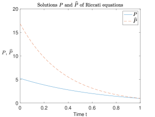
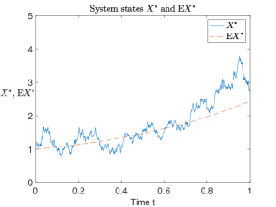
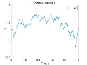
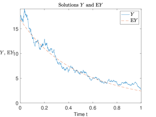
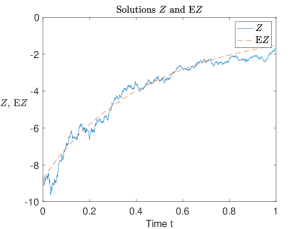
Figure 1: Simulation results for solutions. (a): Solutions $P$ and $\widetilde{P}$ of Riccati equations; (b): Optimal system states $X^{*}$ and $\mathbb{E}X^{*}$; (c): Optimal control $u^{*}$; (d): Solutions $Y$, $\mathbb{E}Y$; (e): Solutions $Z$ and $\mathbb{E}Z$.

Let $\alpha\geq 0$, $\gamma>\max\{\beta,0\}$ and $a(t)\geq(b(t)^{2}\gamma)/(2(\gamma-\beta))$ as before. From another viewpoint, when $\gamma>\beta$, one can check the cost functional is uniformly convex in the control variable, which leads to the unique existence of optimal control. However, the uniform convexity is broken when $\gamma\leq\beta$. One can refer to Sun [26] for more details on this viewpoint.

5.3 An example with negative definite cost weighting of control

In this subsection, we study Example 1.2 presented in Section 1. Firstly, we obtain the optimal controls in open-loop form and closed-loop, respectively. Secondly, the explicit solutions of MF-FBSDE and Riccati equations are presented. Consider the following system

$$\left\{\begin{aligned} dX(t)&=\big{\{}\alpha(t)X(t)+\widetilde{\alpha}(t)\mathbb{E}[X(t)]\big{\}}dt+\beta(t)u(t)dW(t),\\ X(0)&=x,\end{aligned}\right.$$

and the cost functional

$$J(x;u(\cdot))=\mathbb{E}\int_{0}^{T}\big{\{}\gamma(t)X^{2}(t)+\widetilde{\gamma}(t)(\mathbb{E}[X(t)])^{2}-\theta(t)u^{2}(t)\big{\}}dt+G\mathbb{E}[X^{2}(T)].$$

Here, assume that all the coefficients are deterministic. Moreover, $\alpha(\cdot)$, $\widetilde{\alpha}(\cdot)$, $\beta(\cdot)$, $\widetilde{\beta}(\cdot)$, $\gamma(\cdot)$, $\widetilde{\gamma}(\cdot)$ are non-negative. In particular, $\theta(\cdot)$ is positive but not be too large, and satisfies

$$\theta(t)<G\beta^{2}(t)e^{\int_{0}^{T}2\alpha(s)ds}-\int_{0}^{T}\gamma(s)e^{\int_{t}^{s}2\alpha(\tau)d\tau}ds,$$

and $G$ is non-negative. The corresponding Riccati equations follow

$$\left\{\begin{aligned} &~{}\dot{P}(t)+2\alpha(t)P(t)+\gamma(t)=0,\\ &~{}P(T)=G,\\ &~{}\beta^{2}(t)P(t)-\theta(t)>0,\end{aligned}\right.$$

and

$$\left\{\begin{aligned} &~{}\dot{\widehat{P}}(t)+2[\alpha(t)+\widetilde{\alpha}(t)]\widehat{P}(t)+\gamma(t)+\widetilde{\gamma}(t)=0,\\ &~{}\widehat{P}(T)=G.\end{aligned}\right.$$

A short calculation yields

$$P(t)=Ge^{\int_{0}^{T}2\alpha(s)ds}-\int_{0}^{T}\gamma(s)e^{\int_{t}^{s}2\alpha(\tau)d\tau}ds,$$

and

$$\widehat{P}(t)=Ge^{\int_{0}^{T}2(\alpha(s)+\widetilde{\alpha}(s))ds}-\int_{0}^{T}(\gamma(s)+\widetilde{\gamma}(s))e^{\int_{t}^{s}2(\alpha(\tau)+\widetilde{\alpha}(\tau))d\tau}ds.$$

We choose $(P(\cdot),\widehat{P}(\cdot))$ as the relaxed compensator. This problem is well-posed.

From Theorem 4.5, the closed-loop optimal control is taken by $u^{*}(t)=0$. Also, from Theorem 4.4, the open-loop optimal control can be presented by

$$u^{*}(t)=\frac{\beta(t)}{\theta(t)}Z(t),$$ (60)

where $Z(\cdot)$ is determined by

$$\left\{\begin{aligned} dX(t)&=\big{\{}\alpha(t)X(t)+\widetilde{\alpha}(t)\mathbb{E}[X(t)]\big{\}}dt+\frac{\beta^{2}(t)}{\theta(t)}Z(t)dW(t),\\ dY(t)&=-\big{\{}\alpha(t)Y(t)+\widetilde{\alpha}(t)\mathbb{E}[Y(t)]+\gamma(t)X(t)+\widetilde{\gamma}(t)\mathbb{E}[X(t)]\big{\}}dt+Z(t)dW(t),\\ X(0)&=x,~{}~{}~{}Y(T)=GX(T).\end{aligned}\right.$$ (61)

Comparing two forms of optimal control, we get $Z(\cdot)=0$.

Next, we solve $\mathbb{E}[X(t)]$ and $X(t)$ from (61), there are

$$\mathbb{E}[X(t)]=xe^{\int_{0}^{t}\big{(}\alpha(s)+\widetilde{\alpha}(s)\big{)}ds}$$

and

$$X(t)=xe^{\int_{0}^{t}\alpha(s)ds}\big{(}1+\int_{0}^{t}\widetilde{\alpha}(s)e^{\int_{0}^{s}\widetilde{\alpha}(\tau)d\tau}ds\big{)}.$$ (62)

It follows from (24) in Proposition 3.4 that

$$Y(t) =\big{(}Ge^{\int_{0}^{T}2\alpha(s)ds}-\int_{0}^{T}\gamma(s)e^{\int_{t}^{s}2\alpha(\tau)d\tau}ds\big{)}(X(t)-\mathbb{E}[X(t)])$$ (63)

$$~{}~{}~{}+\big{(}Ge^{\int_{0}^{T}2(\alpha(s)+\widetilde{\alpha}(s))ds}-\int_{0}^{T}(\gamma(s)+\widetilde{\gamma}(s))e^{\int_{t}^{s}2(\alpha(\tau)+\widetilde{\alpha}(\tau))d\tau}ds\big{)}\mathbb{E}[X(t)]$$

$$=xe^{\int_{0}^{t}\alpha(s)ds}\big{(}Ge^{\int_{0}^{T}2\alpha(s)ds}-\int_{0}^{T}\gamma(s)e^{\int_{t}^{s}2\alpha(\tau)d\tau}ds\big{)}\big{(}1+\int_{0}^{t}\widetilde{\alpha}(s)e^{\int_{0}^{s}\widetilde{\alpha}(\tau)d\tau}ds-e^{\int_{0}^{t}\widetilde{\alpha}(s)ds}\big{)}$$

$$~{}~{}~{}+xe^{\int_{0}^{t}\big{(}\alpha(s)\widetilde{\alpha}(s)\big{)}ds}+\big{(}Ge^{\int_{0}^{T}2(\alpha(s)+\widetilde{\alpha}(s))ds}-\int_{0}^{T}(\gamma(s)+\widetilde{\gamma}(s))e^{\int_{t}^{s}2(\alpha(\tau)+\widetilde{\alpha}(\tau))d\tau}ds\big{)}.$$

Now, it follows from (62), (63) and $Z(\cdot)=0$ that $(X(\cdot),Y(\cdot),Z(\cdot))$ is the solution to (61).

References

- [1] Ahmed, N. U. & X. Ding (1995). A semilinear McKean-Vlasov stochastic evolution equation in Hilbert space. Stochastic Processes and their Applications, 60, 65-85.
- [2] Ahmed, N. U. (2007). Nonlinear diffusion governed by McKean-Vlasov equation on Hilbert space and optimal control. SIAM Journal on Control and Optimization, 46, pp. 356-378.
- [3] Ait Rami, M., Moore, J. B. & Zhou, X. Y. (2001). Indefinite stochastic linear quadratic control and generalized differential Riccati equation. SIAM Journal on Control and Optimization, 40, 1296-1311.
- [4] Andersson, D. & Djehiche, B. (2011). A maximum principle for SDEs of mean-field type. Applied Mathematics and Optimization, 63, 341-356.
- [5] Barreiro-Gomez, J., Duncan, T. E. & Tembine, H. (2019). Linear-quadratic mean-field-type games: jump-diffusion process with regime switching. IEEE Transactions on Automatic Control, 64, 4329-4336.
- [6] Barreiro-Gomez, J., Duncan, T. E., Pasik-Duncan B. & Tembine, H. (2020). Semiexplicit Solutions to Some Nonlinear Nonquadratic Mean-Field-Type Games: A Direct Method. IEEE Transactions on Automatic Control, 65, 2582-2597.
- [7] Bensoussan, A., Yam, S. & Zhang, Z. (2015). Well-posedness of mean-field type forward–backward stochastic differential equations. Stochastic Processes and their Applications, 125, 3327-3354.
- [8] Borkar, V. S. & Kumar, K. S. (2010). McKean-Vlasov limit in portfolio optimization. Stochastic Analysis and Applications, 28, 884-906.
- [9] Buckdahn, R., Djehiche, B., Li, J. & Peng, S. (2009). Mean-field backward stochastic differential equations: a limit approach. Annals of Probability, 37, 1524-1565.
- [10] Buckdahn, R., Djehiche, B. & Li, J. (2011). A General stochastic maximum principle for SDEs of mean-field type . Applied Mathematics and Optimization, 64, 197-216.
- [11] Chan, T. (1994). Dynamics of the McKean-Vlasov equation, Annals of Probability, 22, pp. 431-441.
- [12] Chen, S., Li, X. & Zhou, X. (1998). Stochastic linear-quadratic regulators with indefinite control weight costs. SIAM Journal on Control and Optimization, 36, 1685-1702.
- [13] Crisan, D. & Xiong, J. (2010). Approximate McKean-Vlasov representations for a class of SPDEs. Stochastics, 82, 53-68.
- [14] Duncan, T. E. & Tembine, H. (2018). Linear-quadratic mean-field-type games: a direct method. Games, Pages 18.
- [15] Duncan, T. E.; & Pasik-Duncan, B. (2017). A direct approach to linear-quadratic stochastic control. Opuscula Mathematica, 37, 821-827.
- [16] Huang, M., Malhame, R. P. & Caines, P. E. (2006). Large population stochastic dynamic games: closed-loop McKean-Vlasov systems and the Nash certainty equivalence principle, Communications in Information and Systems, 6, 221-252.
- [17] Huang, J., Li, X. & Yong, J. (2015). A linear-quadratic optimal control problem for mean-field stochastic differential equations in infinite horizon. Mathematical Control and Related Fields, 5, 97-139.
- [18] Huang, J. & Yu, Z. (2014). Solvability of indefinite stochastic Riccati equations and linear quadratic optimal control problems. Systems and Control Letter, 68, 68-75.
- [19] Kohlmann, M. & Zhou, X.Y. (2000). Relationship between backward stochastic differential equations and stochastic controls: a linear-quadratic approach. SIAM Journal on Control and Optimization, 38, 1392-1407.
- [20] Kotelenez, P. M. & Kurtz, T. G. (2010). Macroscopic limit for stochastic partial differential equations of McKean-Vlasov type. Probability Theory and Related Fields, 146, 189-222.
- [21] Li, D. & Zhou, X. Y. (2000). Continuous-time mean-variance portfolio selection: a stochastic LQ framework. Applied Mathematics and Optimization, 42, 19-33.
- [22] Li, X., Sun, J. & Yong, J. (2016). Mean-field stochastic linear quadratic optimal control problems: closed-loop solvability. Probability, Uncertainty and Quantitative Risk, 1, 1-22.
- [23] Markowitz, H. (1952). Portfolio selection. The Journal of Finance, 7, 77-91.
- [24] Markowitz, H. (1959). Portfolio selection: efficient diversification of investment. John Wiley and Sons, New York.
- [25] Qian, Z. & Zhou, X. (2013) Existence of solutions to a class of indefinite stochastic Riccati equations. SIAM Journal on Control and Optimization,51, 221-229.
- [26] Sun, J. (2017). Mean-field stochastic linear quadratic optimal control problems: Open-loop solvabilities. ESAIM: Control, Optimisation and Calculus of Variations, 23, 1099-1127.
- [27] Sun, J. & Wang, H. (2019). Mean-field stochastic linear-quadratic optimal control problems: weak closed-loop solvability. arXiv preprint arXiv:1907.01740.
- [28] Wei, Q., Yong, J. & Yu, Z. (2019). Linear quadratic stochastic optimal control problems with operator coefficients: open-loop solutions. ESAIM: Control, Optimisation and Calculus of Variations, 25, 17-38.
- [29] Yong, J. (2013). Linear-quadratic optimal control problems for mean-field stochastic differential equations. SIAM Journal on Control and Optimization, 51, 2809-2838.
- [30] Yong, J. (2017). Linear-quadratic optimal control problems for mean-field stochastic differential equations—time-consistent solutions. Transactions of The American mathematical society, 369, 5467-5523.
- [31] Yong, J. & Zhou X. (1999). Stochastic controls: Hamiltonian systems and HJB equations. New York, NY, USA: Springer-Verlag.
- [32] Yu, Z. (2013). Equivalent cost functionals and stochastic linear quadratic optimal control problems. ESAIM: Control, Optimisation and Calculus of Variations, 19, 78-90.