Ethnic Groups’ Access to State Power and Group Size

Abstract

Many countries are ethnically diverse. However, despite the benefits of ethnic heterogeneity, ethnic-based political inequality and discrimination are pervasive. Why is this? This study suggests that part of the variation in ethnic-based political inequality depends on the relative size of ethnic groups within each country. Using group-level data for 569 ethnic groups in 175 countries from 1946 to 2017, I find evidence of an inverted-U-shaped relationship between an ethnic group’s relative size and its access to power. This single-peaked relationship is robust to many alternative specifications, and a battery of robustness checks suggests that relative size influences access to power. Through a very simple model, I propose an explanation based on an initial high level of political inequality, and on the incentives that more powerful groups have to continue limiting other groups’ access to power. This explanation incorporates essential elements of several existing theories on the relationship between group size and discrimination, and suggests a new empirical prediction: the single-peaked pattern should be weaker in countries where political institutions have historically been less open. This additional prediction is supported by the data.

Keywords: Access to State Power, Ethnic Groups, Group Size.
JEL classification: H41, O17

1 Introduction

Many countries are ethnically diverse, regardless of their level of development. Despite the benefits of ethnic heterogeneity, ethnic-based political inequality and discrimination are pervasive. Why is this? This study suggests that part of the variation in ethnic-based political inequality depends of the relative size of ethnic groups within a country.

Using group-level data for 569 ethnic groups in 175 countries from 1946 to 2017, I find evidence of an inverted-U-shaped relationship between the relative size of an ethnic group and its access to power. This single-peaked relationship is robust to many alternative specifications, which include group fixed effects, time-varying group-specific controls, country-time fixed effects and group-specific linear trends. This relationship is also robust to using lagged relative group size as an instrument for its current value.

Though caution is necessary in interpreting the results as causal, they are consistent with relative group size affecting access to power. Taking this into consideration, I propose an explanation based on an initial high level of political inequality, and on the incentives that more powerful groups have, ex ante, to continue limiting other groups’ access to power. Through a very simple model, I argue that these incentives crucially depend on the relative size of politically marginalized groups, and follow an inverted-U-shaped pattern. First, when a politically marginalized group is very small, the group tends to be irrelevant, so more powerful groups have little incentive to cede any control to this small group. Second, when a politically marginalized group is relatively large, individuals in very powerful — but also relatively small — groups greatly value a government controlled by their own group, as it allows them to extract very high per capita rents. Therefore, individuals in small powerful groups do not have incentives to share power because it would limit their ability to keep rents for themselves. Only when a politically excluded group is neither very big nor very small can it expect to receive greater access to power; the excluded group is big enough to potentially overthrow the government if it isn’t voluntarily given access to power, but small enough that it wouldn’t detract too much from the incumbent group’s ability to extract rents in a power-sharing arrangement.

The model I propose to explain the inverted-U relationship between group size and access to power leads to a new empirical prediction that identifies a crucial role of the persistence of political institutions: the single-peaked pattern should be weaker in countries where political institutions have historically been less open. Insofar as undemocratic institutions tend to persist, in countries with political institutions that have traditionally been less open, any increase in the de jure access to power of politically marginalized groups might be seen as less threatening by more powerful groups. Thus, insofar as the costs of maintaining the status quo increase with the size of marginalized groups, in countries where political institutions have historically been less open, the model predicts a monotonically increasing relation between group size and access to power.

Using PolityIV’s measures of openness and competitiveness of executive recruitment as a proxy for the openness of political institutions, I find evidence consistent with this additional prediction: the inverted-U relationship between group size and access to power is specific to countries where political institutions have been more open in the past; in countries with less open political institutions, this relationship tends to be monotonically increasing.

The rest of the paper is organized as follows. Section 2 discusses the existing literature on the relationship between political exclusion and group size. The data and empirical strategy are discussed in Section 3. The main results are presented in Section 4. Section 5 presents the model, and Section 6 provides additional evidence related to the role of the persistence of political institutions. Section 7 concludes.

2 Related literature

The sociology and economics literatures have developed distinct approaches to examining the relationship between group discrimination and group size. The classical sociological approach identifies the size of the groups as a crucial factor in explaining how individuals in dominant groups perceive potential threats posed by individuals in other groups. This literature has proposed two hypotheses about the specific relationship between this perception and the size of the subordinate groups. First, it may be that the larger the size of a subordinate group, the more individuals in a dominant group perceive the subordinate group as a threat to their economic and social privileges and, therefore, the higher their motivation to discriminate against the subordinate group (see for instance Blumer 1958 or Blalock 1967). Second, it may be that the larger the relative size of a subordinate group, the greater the opportunity for positive intergroup contact, which reduces the motivation for individuals in the dominant group to discriminate against individuals in the subordinate group (see for instance Allport 1954 or Pettigrew 1998). The empirical evidence for these two theories is inconclusive (see Schlueter and Scheepers (2010) for a critical review), with problems related to identification and external validity.

The economics literature relating discrimination and group size is less abundant, and focuses on discrimination in labor markets and segregation. Departing from a standard model of statistical discrimination in labor markets, Moro and Norman (2004) propose a theoretical extension that examines how group size affects conflicting interests between groups. Specifically, they find that as the marginalized group grows, the per capita gains from discrimination for individuals in the dominant group also grow, as do the incentives of individuals in the subordinate group to invest in human capital. This makes it harder to sustain a discriminatory equilibrium, and suggests one rationale for apartheid or other discriminatory measures; however, Moro and Norman (2004) do not model this explicitly.

Eeckhout (2006) proposes a model of segregation in which segregation can make minority groups worse off while making the majority better off, so that any change in equilibrium that eliminates segregation will make the majority worse off. Even though it is not explicitly modeled, Eeckhout’s main result is consistent with Moro and Norman’s rationale for the existence of institutional devices to ensure that the preferred equilibrium for the group with political control is realized.

This paper seeks to contribute to the sociological literature by providing new and relatively well-identified evidence about the relationship between group discrimination and group size, with a specific focus on the access to power of individuals in subordinate groups (rather than on out-group attitudes). In addition, this paper proposes a new and very stylized micro-funded theory that allows for the possibility of a non-monotonic relationship. This paper seeks to contribute to the economics literature by providing evidence about the relationship between group discrimination and group size, and on the role of institutional mechanisms that affect this relationship.

3 Empirical specification and identification

3.1 Data

I study 569 ethnic groups in 175 countries from 1946 to 2017. The baseline specification is divided into 10-year sub-periods (starting in 1945) to account for potential lags in the relationship between group size and group access to state power. To construct observations for each sub-period, I take an average of the annual data from that sub-period.

The analysis is based on the Ethnic Power Relations (EPR) Core Dataset 2018, which identifies all politically relevant ethnic groups and their access to state power in every country of the world from 1946 to 2017 (Vogt et al., 2015). It provides annual data on politically relevant ethnic groups, their relative sizes as a share of the total population, and their access to executive state power in all countries with a population of at least 250,000.

The EPR dataset characterizes an ethnic group as politically relevant if at least one significant political actor claims to represent the interests of that group in the national political arena, or if group members are systematically and intentionally discriminated against in public politics. The EPR measures access to power with a roughly ordinal scale composed of three main categories (and several subcategories), depending on whether a group controls power alone, shares power with other ethnic groups, or is excluded from executive state power. Specifically, the EPR measures power access according to the following categories and subcategories:

• The group rules alone:

  • Monopoly – Members hold monopoly power in the executive.

  • Dominance – Members hold dominant power in the executive.

• The group shares central power:

  • Senior partner – Members participate as senior partners in a formal or informal power-sharing arrangement.

  • Junior partner – Members participate as junior partners in government.

• The group is excluded from central power:

  • Powerless – Members do not have influence on decision-making at the national level of executive power, but are not explicitly discriminated against.

  • Discrimination – Members are subjected to active, intentional and targeted discrimination by the state, with the intent of excluding them from political power.

  • Self-exclusion (or separatist autonomy) – Members have excluded themselves from central state power.

  • Irrelevance – Members’ ethnicity is not politicized (but the members comprise a sufficiently large group).

Although these categories are qualitative, they have a clear hierarchy: “monopoly” means more access to power than “dominance,” which is better than sharing power. For groups that are excluded, being powerless plausibly implies having more access to power than being irrelevant or self-excluded, and the worst scenario is likely discrimination. I exploit this implicit order to construct a scale of access to power from 0 to 5.

Table I:

EPR classification	Access to power score
Monopoly	5
Dominance	4
Senior partner	3
Junior partner	2
Powerless/Irrelevance/Self-exclusion	1
Discrimination	0

The index in Table I relies on two main assumptions. First, groups that are discriminated against have less access to central power than groups that are irrelevant, powerless or self-excluded. The justification for this assumption is that being explicitly discriminated against implies greater costs — for accessing power — than being powerless, irrelevant or self-excluded. Second, groups that are powerless, irrelevant or self-excluded have the same (low) level of access to central power. The justification for this assumption is based on the notion of irrelevance: if a group is self-excluded or powerless, dominant groups will likely expect that the other group’s members will be unable to gain access to central power.

The other main dataset used in the paper is the Polity IV dataset, which evaluates the openness and competitiveness of countries’ political institutions. Specifically, I use Polity IV’s “Openness of Executive Recruitment” and “Competitiveness of Executive Recruitment” to measure how politically open and competitive a country’s institutions are in a given year (or decade).

3.2 Empirical Strategy and Identification

As previously mentioned, there is no consensus among scholars about the relationship between group size and access to power. My empirical analysis allows for the possibility of either a negative or positive relationship.

In the main specification, I model the outcome $y_{gct}$ (my index of access to central power based on the EPR power access characterization) of group $g$ in country $i$ and 10-year period $t$ as

$$access\_to\_power_{gct}=\alpha+\beta_{1}\times size_{gct}+\beta_{2}\times size^{2}_{gct}+\gamma_{ct}+\eta_{g}+\epsilon_{gct}$$ (1)

where $size_{gct}$ is the relative size of $g$ in country $i$ and period $t$, $size^{2}_{gct}$ is the square of this size, $\gamma_{ct}$ are country/period fixed effects, $\eta_{g}$ are group fixed effects and $\epsilon_{gct}$ is the error term. In some specifications, I also add group-specific linear trends, and control for the presence of each group in other countries (which varies at the group $\times$ 10-year level). The two coefficients of interest are $\beta_{1}$ and $\beta_{2}$, which are associated with the relative size of the groups; $\beta_{2}$ is introduced to allow for a nonlinear relationship.

With respect to identification, since the baseline specification (1) includes country/period fixed effects, it controls for any omitted variable varying at the country $\times$ 10-year level. In addition, the inclusion of group-specific linear trends helps control for any omitted linear trend that varies at the group level. Finally, note that the control for the presence of each group in other countries accounts for a potentially omitted (and crucial) channel: a group may have less (or more) access to central power because its members were (or haven’t been) forced to migrate to other countries, and this migration (or lack of it) may also explain the small (or large) group size.

Simultaneity is also a concern in (1) if, for instance, groups with less access to power have lower fertility rates. To address this, I first replace the explanatory variables (group size and the square of group size) with their lagged values. Second, I instrument group size (and the square of group size) with a lagged group size (and a lag of the squared group size). As long as the lagged values for group size do not themselves exert a direct effect on power access, this second alternative specification provides an effective estimation strategy.

Even though I recognize that fixed effects regressions (such as (1)) cannot necessarily estimate the causal effect of group size on power access (e.g. there may be still omitted variables varying non-linearly at the group $\times$ period level that are weakly correlated with a group’s presence in other countries), the results are robust to many alternative specifications, which significantly alleviates these concerns.

4 Baseline empirical results

Figure I shows, for each non-dominant minority group in each 10-year period, the correlation between the group’s access to power score and the relative size of the group (i.e. the group’s membership as a proportion of the country’s population). It shows a clear inverted-U shape.

Table Graphs and Tables reports the estimated coefficients for variations of the model in Eq. (1). The specification in column (1) does not include any controls or fixed effects, and corresponds to the specification used in Figure I. Column (2) includes country and 10-year-period fixed effects, and column (3) adds country/10-year period fixed effects. Columns (4) and (5) include group fixed effects and group-specific linear trends. In all the specifications in Table Graphs and Tables, the estimated coefficients for $\beta_{1}$ are positive, the coefficients for $\beta_{2}$ are negative, and all are individually and jointly significant. In addition, the peak is located at 0.47, which lies comfortably within the range of values for relative group size (i.e, between 0 and 1). Thus, these results confirms the inverted-U shape in Figure I.

I also provide results for several additional specifications to verify the robustness of the results in Table Graphs and Tables. First, instead of averaging annual results over a 10-year period, I use one observation from within each 10-year period (e.g one observation every tenth year). These estimates are shown in Panel A of Table LABEL:integrVSsizeOLSav10yrrobustness1_tab. Second, instead of using 10-year periods, I use a five-year panel. These estimates are shown in Panel B of Table LABEL:integrVSsizeOLSav10yrrobustness1_tab. Third, instead of the continuous measure for access to state power, I use a dichotomous measure of access to power that is equal to 1 if a group is not excluded from central power and 0 if it is excluded. These estimates are shown in Panel C of Table LABEL:integrVSsizeOLSav10yrrobustness1_tab. In all three additional specifications, the results from Table Graphs and Tables hold, i.e. all specifications show a clear inverted-U-shaped relationship between the relative size of a group and its level of access to central power.

In interpreting causality, we must be cautious of reverse causality bias: a group’s access to power may affect its relative size (e.g. groups that are discriminated against may migrate to other countries and/or have lower fertility rates). In addition, groups that differ in relative size might also differ in other unobserved and non-linearly time-varying characteristics that affect their access to central power (e.g. members of large groups may receive support from exiles in other countries, and this may improve their chances to gaining access to central power). If this is the case, the previous results may be affected by omitted-variable bias.

Table LABEL:integrVSsizeOLSav10yrlagIVcontrol_tab addresses these potential issues. Columns (1) to (3) of panel A consider specifications that use lagged values of group size as an independent variable instead of current group size. Columns (4) and (5) of panel A consider specifications that use the lagged values of relative group size as instruments for the contemporaneous values. Under certain conditions, these two strategies help to avoid the inconsistency problems associated with simultaneity (see Reed, 2015). All the estimates are virtually the same as those in Table Graphs and Tables, which indicates that simultaneity is likely not a problem.

Omitted-variable bias may be less worrisome given the different fixed effects included in the baseline specifications. In addition, the specifications in panel B of Table LABEL:integrVSsizeOLSav10yrlagIVcontrol_tab add one crucial covariate: the presence of members of the same group in other countries. All the estimates remain the same whether we consider contemporaneous values for the relative size (columns (1) to (3)), lagged values (column (4)), or lagged values as instruments for the contemporaneous values (column (5)).

While one must be cautious in claiming that the estimates in Tables Graphs and Tables to LABEL:integrVSsizeOLSav10yrlagIVcontrol_tab are caused by purely exogenous shocks, the fact that the results in Table Graphs and Tables are robust to all the specifications in Table LABEL:integrVSsizeOLSav10yrlagIVcontrol_tab guards against the most obvious forms of endogeneity.

5 Explaining the inverted U: A simple model

In this section, I propose an explanation of the single-peaked relationship between access to central power and relative group size. I use a very simple stylized model in which one group, with an ex ante monopoly of political power, decides whether to continue limiting other groups’ access to central power.

5.1 Set-up

Consider a society composed of individuals who belong to n internally homogenous groups. Let $N$ be the total number of individuals in the society, with $N_{i}$ representing the number of individuals in group $i$, so that $\sum_{i=1}^{n}N_{i}=N$. There are two time periods, each with a government that may be controlled by a single group or by several groups. Assume that in the first period, one group (or a cluster of groups) fully controls the government and decides whether or not to continue limiting other groups’ access to power in the second period. Without loss of generality, we set $n=2$, and assume that group 1 has an ex ante monopoly over political power in period 1. Group 2 can be interpreted as a cluster of groups with limited access to power in period 1; de jure, this group is totally excluded from government decisions in period 1 (and potentially in period 2). If group 2’s access to power in period 2 is not restricted, both group 1 and group 2 will participate in the period-2 government. Crucially, I assume that if group 2’s access to power in period 2 is not de jure limited, its level of control over the period-2 government will be proportional to its share of the population. Specifically, let $s_{i}$ denote group $i$’s level of control over the period-2 government, and assume that

$$s_{i}=\frac{N_{i}}{\sum_{j=1}^{2}N_{j}}.$$ (2)

As previously mentioned, the analysis focuses on group 1’s decision about whether or not to, de jure, limit group’s 2 access to power in period 2. This decision depends on the benefits that individuals in group 1 obtain from a government fully or partially controlled by their own group. Specifically, I assume that the government has an exogenously determined budget that it divides and transfers to individuals using the following approach. First, each group that participates in the government receives an allocation of the budget proportional to that group’s level of control of the government. Second, the budgetary allocation for that group is divided equally among the group’s members. In other words, if group $i$ has monopoly control of the government, and if the per capita value of the government budget is normalized to unity, then each member of this group will receive $N/N_{i}$.

Individuals use their government transfer to purchase a private good in period 2, from which they derive utility that increases linearly in their consumption of the private good. More precisely, we define the overall payoff to an individual in group 1 when group’s 2 access to power is not restricted as

$$s_{1}(N/N_{1}).$$ (3)

When group 1 decides to restrict group’s 2 access to power, I assume that group 2 attempts to overthrow group 1’s government, which results in a costly contest between the two groups. The group that wins this contest fully controls the government in period 2. The success of each group depends on its relative size and on its capacity to coordinate its actions. Specifically, I assume the following contest function:

$$p_{i}=\frac{N_{i}+a_{i}}{\sum_{j=1}^{2}(N_{j}+a_{j})}$$ (4)

where $a_{i}\geq 0$ for $i=1,2$ is a parameter that captures how sensitive a group’s probability of success is to the group’s relative population. This can be interpreted as the ability of each group to solve the collective-action problem.

I model the costs of the conflict as follows. I assume that a fraction of the government budget is destroyed due to violence, and only the reminder can be divided among the members of the winning group. The fraction of the budget that is destroyed is assumed to be proportional to the relative size of group 2, since the bigger the group without political rights, the greater its capacity to cause turbulence and destruction. I therefore summarize the overall payoff to an individual in group 1 when group’s 2 access to power is limited as

$$p_{i}(N/N_{1})(1-\lambda(N_{2}/N))$$ (5)

where $\lambda(N_{2}/N)$ is the fraction of the government budget that is destroyed, and $\lambda\in(0,1)$ is a parameter that captures the marginal increase in the level of destruction as the relative size of group 2 increases.

Finally, I make two assumptions about the parameters $\lambda$, $a_{1}$ and $a_{2}$. First, I assume that $a_{1}>a_{2}$, and normalize $a_{2}=0$, with which $a_{1}>0$. As discussed in footnote 22, this implies that the de facto power of group 1 in period 2 is greater than that of group 2. This assumption can be justified by the fact that group 1 had the monopoly of power in period 1, so it is plausible that this group, in period 2, has more resources to invest in increasing its de facto political power.

Second, I assume that

$$\ThisStyle{\lambda\mathord{\stretchto{\raisebox{2.3pt}{$\SavedStyle/$}}{}}(1-\lambda)}>a_{1}.$$ (6)

By implying that the costs of conflict are sufficiently high and that the de facto power of group 1 is sufficiently low, this second assumption basically guarantees that limiting group 2’s access to power is not a dominant strategy for group 1.

5.2 Equilibrium

The main objective of this section is to propose an explanation for the empirical relationship between access to power and relative size found in Section 4. This section examines the conditions under which individuals in group 1 decide whether to limit group 2’s access to power in period 2 and, specifically, how those conditions depend on the relative size of the two groups.

From the previous analysis, it is clear that group 1 will not give group 2 access to power in period 2 when the expression in (5) is greater than the expression in (3), i.e. when

$$p_{i}(N/N_{1})(1-\lambda(N_{2}/N))\geq s_{1}(N/N_{1}).$$ (7)

To facilitate the exposition and interpretation of the results, I normalize the population to 1 (i.e. $N=1$), and define $\delta$ as the relative size of group 2 (so $N_{1}=1-\delta$ and $N_{2}=\delta$). Thus, replacing the expressions for $s_{i}$ and $p_{i}$ in (7) and rearranging, it is easy to see that (7) is equivalent to

$$\frac{(1-\delta+a_{1})}{(1+a_{1})}\frac{(1-\lambda\delta)}{(1-\delta)}-1\geq 0.$$ (8)

The expression in (8) constitutes the main finding of this section. Importantly, it entails an inverted-U relationship between group 2’s relative size (i.e. $\delta$) and its access to central power. This result is summarized in the following proposition:

Proposition 1.

Consider the above-described game. In equilibrium, the relationship between access to central power for a group with an ex ante limited access and its relative size ($\delta$) follows an inverted-U pattern: this group’s access to central power is expected to be lower for smaller and larger values of $\delta$, and higher for intermediate values of $\delta$.

Proof.

See the Appendix. ∎

The inverted-U shape can be explained as follows. First, when the relative size of group 2 is very small, individuals in group 1 have few incentives to increase group 2’s access to power because the cost of maintaining the status quo, which benefits group 1, is small: the ensuing contest with group 2 is expected to be minimally destructive and group 1’s chance of success is very high. As the relative size of group 2 increases, a contest becomes more destructive, so the period-2 budget associated with this scenario is reduced; this gives individuals in group 1 an incentive to increase group 2’s access to power. Finally, when the relative size of group 2 is very big, this means group 1 is relatively very small, which implies that individuals in group 1 greatly value a government fully controlled by their group (because the per capita transfers they receive are very large). In these circumstances, individuals in group 1 have few incentives to increase group 2’s access to power, even though this implies that the government will have a significantly reduced budget in period 2 (which is mitigated somewhat by a contest function that is biased in favor of group 1).

Importantly, note that the U-shaped relationship described in Prop. 1 is consistent with the empirical evidence in Section 3. In particular, it rationalizes the results in Figure I and Columns (1) to (6) in Table Graphs and Tables. It is also important to note that even though the explanation I propose is new, it is consistent with the main predictions of the existing theoretical literature on group discrimination. Specifically, it is consistent with the idea that the smaller a minority, the more it suffers (Eeckhout, 2006), and the larger a minority, the more likely the coercive measures against it (Moro and Norman, 2004), and the greater the antipathy felt towards it (Blumer, 1958; Blalock, 1967; Oliver and Wong, 2003). One of the contributions of this paper is to propose a very simple mechanism that explains (and tests) both predictions.

5.3 Persistence of political institutions

In the last subsection it was assumed that if group 2 is given access to power in period 2, its level of power will be proportional to its size. As mentioned in footnote 19, this means that the institutions that affect group 2’s access to political power can transition from being completely closed to being completely open. In this subsection, I remove this assumption to allow for the possibility that institutions in period 2 are biased in favor of group 1 even if group 2’s access to power is not limited. The motivation behind this extension is based on the idea that institutions tend to persist for long periods (Acemoglu et al., 2001, 2002; Banerjee and Iyer, 2005).

Specifically, I assume that when group 2’s access to power is not de jure limited, the participation of group 2 in the period-2 government is given by

$$q_{2}=\gamma s_{2}$$ (9)

where $\gamma\in[0,1]$ is a parameter that measures how unbiased political institutions are expected to be in period 2. Since period-1 political institutions are assumed to be very biased in favor group 1, $\gamma$ can be understood as the inverse of how persistent institutions are.

From (9), note that since $q_{1}=1-q_{2}$, we have that $q_{1}=\gamma s_{1}+1-\gamma$. From these expressions, note that when $\gamma=1$, $q_{i}=s_{i}$ for $i=1,2$, which corresponds to the scenario examined in the last subsection. Importantly, note that $q_{1}\geq s_{1}$, $q_{2}\leq s_{2}$, and that as $\gamma$ decreases $q_{1}$ increases, meaning that group 1’s level of control in the period-2 government can be disproportionally larger despite the fact that group 2’s access to power is not de jure limited.

Replacing $q_{2}$ in (8) and rearranging, it is easy to see that we have

$$\frac{(1-\delta+a_{1})}{(1+a_{1})}\frac{(1-\lambda\delta)}{(1-\delta)}-\frac{(1-\gamma\delta)}{(1-\delta)}\geq 0.$$ (10)

By analyzing (10), the following proposition summarizes how the results in Prop. 1 change when institutions in period 2 are expected to be biased in favor of group 1, even though both groups have access to power.

Proposition 2.

Consider the above-described game. In equilibrium, if political institutions are sufficiently persistent, then the relationship between a group’s access to central power and its relative size does not follow an inverted-U pattern and, more specifically, the larger a group’s relative size, the more likely it will have access to power.

Proof.

See the Appendix ∎

The intuition behind Prop. 2 is straightforward: the more biased institutions are expected to be in favor of group 1, the less costly it is for group 1 to give group 2 access to power, particularly when group 2 is relatively large. In addition, and importantly, Prop. 2 establishes a new empirical prediction: the inverted-U relationship between relative size and access to power crucially depends on the historical quality of institutions; for historically closed political institutions, it is more likely that this relationship, if existent, is positive (rather than non-monotonic). In the next section I examine the empirical plausibility of this new prediction.

6 Additional evidence

This section empirically examines whether the results in Section 4 depend on the historical level of openness of the political institutions, as predicted in Section 5. To measure the openness of political institutions, I use two proxies from PolityIV. First, I use a variable called “Openness of Executive Recruitment (xropen).” This variable measures “the extent that the politically active population has an opportunity, in principle, to attain the position through a regularized process” (see Marshall and Jaggers, 2019). It ranges from 0 to 4, with 4 representing the most open institutions. Second, I use a variable called “Competitiveness of Executive Recruitment (xrcomp),” which measures “the extent that prevailing modes of advancement give subordinates equal opportunities to become superordinates.” This variable ranges from 0 to 3, with 3 representing the most competitive institutions. Since the hypothesis regarding how the level of political openness should affect each group’s access to power is based on the persistence of institutions, I compute, for each country-year, the average for each variable since 1800. Then, I define a dummy variable equal to 1 if, for the case of the variable xropen, its historical average is equal to 4 (which is very close to the median, and represents a highly open system), and for the case of the variable (xrcomp), its historical average is above the median (which represents a highly competitive system).

Table LABEL:integrVSsizeOLSav10yropenness_tab shows estimates of the same specifications used in columns (4) and (5) of Table Graphs and Tables, but distinguishes between countries with high and low historical levels of openness (Panel A), and between countries with high and low historical levels of competitiveness (Panel B). These estimates show that the non-monotonic (inverted-U-shaped) effect of group size on access to power is stronger in countries with historically high levels of openness and competitiveness (columns (1) and (2)), and weaker (and almost nonexistent) in countries that are less open and competitive (columns (3) and (4)). In addition, for countries with historically low levels of openness and competitiveness, the relationship between group size on access to power appears to follow a linear and positive pattern (see column (5)). Table LABEL:integrVSsizeOLSav10yropennesslagIV_tab explores the robustness of the previous results to the use of lagged values for group size as i) independent variables (columns (1) to (3)) and as ii) instruments for the contemporaneous values (columns (4) to (6)). The robustness results are all consistent with those in Table LABEL:integrVSsizeOLSav10yropenness_tab.

Importantly, the results in Tables LABEL:integrVSsizeOLSav10yropenness_tab and LABEL:integrVSsizeOLSav10yropennesslagIV_tab are consistent with the prediction of the model proposed in the Section 5. In particular, they show that as we move from high to low levels of openness, the relationship between group size on access to power passes from having a marked inverted-U shape to being better described as monotonically increasing. As mentioned in the last section, this can be explained by a decrease in the costs (to the group with access to power) associated with not limiting other groups’ access to power.

7 Conclusion

This study examines whether the relative size of ethnic groups within a country affects the extent to which governments limit these groups’ access to central power. Using data at the group level in 175 countries from 1946 to 2017, I find evidence of an inverted-U-shaped relationship between the relative size of groups and their access to central power. This single-peaked relationship is robust to many alternative specifications, and several robustness checks suggest that relative size causes access to power. Through a very simple model, I propose an explanation based on an initial high level of political inequality, and on the incentives that more powerful groups have to continue limiting other groups’ access to power. This explanation incorporates essential elements of existing theories about the relationship between group size and political and social exclusion, and leads to a new empirical prediction: the single-peaked pattern should be weaker in countries where political institutions have been less open in the past. This additional prediction is supported by the data.

Several opportunities exist for future research. One could examine the effect of ethnic groups’ relative size on other — more de facto — forms of political participation, such as the formation of political organizations and participation in protests. It would also be interesting to examine whether other kind of institutions matter (e.g. less formal political institutions and cultural institutions). Finally, there is a question of whether individuals in dominant groups actually agree that the institutions that their groups control limit access to the power of minority groups.

Graphs and Tables

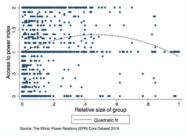
Figure I: Scatter plot of relative size and access to central power

The figure plots a measure of the size of each ethnic group on the x-axis against each group’s access to power score — as defined in Table I — on the y-axis. Each point represents a group over a 10-year period. The quadratic curve that is overlaid is reported in column (1) of Table Graphs and Tables.

Table II: Relative size and access to central power

	Dep. variable: Level of access to central power
	(1)	(2)	(3)	(4)	(5)
Relative size	1.676∗∗∗	1.672∗∗∗	1.672∗∗∗	1.684∗∗∗	1.683∗∗∗
	(0.335)	(0.334)	(0.334)	(0.332)	(0.332)
Relative size squared	-1.782∗∗∗	-1.778∗∗∗	-1.778∗∗∗	-1.790∗∗∗	-1.789∗∗∗
	(0.352)	(0.350)	(0.350)	(0.348)	(0.348)
Joint significance	0.000	0.000	0.000	0.000	0.000
Vertex	0.470	0.470	0.470	0.470	0.470
R-squared	0.058	0.062	0.064	0.071	0.072
Observations	836462	836462	836462	836462	836462

Country fixed effects N Y Y Y Y 10-year period fixed effects N Y Y Y Y Country/period fixed effects N N Y Y Y Group fixed effects N N N Y Y Group-specific linear trends N N N N Y    Notes: All columns report OLS estimates for estimates from Eq (1). The dependent variable in all columns is each ethnic group’s access to power score (as defined in Table I). The sample is limited to groups with a score of 2 or less, and the index is averaged over a 10-year period. In this subsample, the average relative size is 0.117 (with s.d. 0.224) and the average level of access to central power is 1.036 (with s.d. 0.575). Robust standard errors clustered by country are in parentheses. * denotes results are statistically significant at the 10% level, ** at the 5% level, and *** at the 1% level.

Panel B: Using averages over 5-year periods    Relative size 1.642^∗∗∗ 1.638^∗∗∗ 1.637^∗∗∗ 1.650^∗∗∗ 1.649^∗∗∗ (0.342) (0.341) (0.341) (0.339) (0.339) Relative size squared -1.746^∗∗∗ -1.742^∗∗∗ -1.741^∗∗∗ -1.754^∗∗∗ -1.753^∗∗∗ (0.360) (0.358) (0.358) (0.356) (0.356) Joint significance 0.000 0.000 0.000 0.000 0.000 Vertex 0.470 0.470 0.470 0.470 0.470 R-squared 0.054 0.058 0.060 0.067 0.068 Observations 1568532 1568532 1568532 1568532 1568532    Panel C: Dep. var. is prob. of access to power    Relative size 3.083^∗∗∗ 3.078^∗∗∗ 3.077^∗∗∗ 3.086^∗∗∗ 3.086^∗∗∗ (0.278) (0.277) (0.277) (0.276) (0.276) Relative size squared -3.197^∗∗∗ -3.191^∗∗∗ -3.190^∗∗∗ -3.199^∗∗∗ -3.199^∗∗∗ (0.290) (0.289) (0.289) (0.288) (0.288) Joint significance 0.000 0.000 0.000 0.000 0.000 Vertex 0.482 0.482 0.482 0.482 0.482 R-squared 0.305 0.308 0.310 0.312 0.313 Observations 836462 836462 836462 836462 836462 Country fixed effects N Y Y Y Y Period fixed effects N Y Y Y Y Country/period fixed effects N N Y Y Y Group fixed effects N N N Y Y Group-specific linear trends N N N N Y    Notes: All columns report OLS estimates for estimates from Eq (1). The dependent variable in all columns is based on ethnic group’s access to power score (as defined in Table I). The sample is limited to groups with a score of 2 or less. Panel A uses 10-year panel, but rather than averaging the 10-year data, it takes one observation within each sub-period (e.g one every tenth year). In this sample, the average relative size is 0.121 (with s.d. 0.228) and the average level of access to power is 1.023 (with s.d. 0.609). Panel B uses a 5-year panel. In this sample, the average relative size is 0.118 (with s.d. 0.226) and the average level of access to power is 1.030 (with s.d. 0.586). Panel C uses 10-year panel and a dichotomous measure of access to power which is equal to one if the group is not excluded from central power and zero if it is excluded. In this sample, the average probability of not being excluded from central power is 0.216 (with s.d. 0.411). Robust standard errors clustered by country are in parentheses. * denotes results are statistically significant at the 10% level, ** at the 5% level, and *** at the 1% level.

Y Y Y Y Y Country/period fixed effects Y Y Y N Y Group fixed effects N Y Y N N Group-specific linear trends N N Y N N    Panel B:       Baseline specification       Lagged       IV    Relative size 1.679^∗∗∗ 1.684^∗∗∗ 1.683^∗∗∗ 1.706^∗∗∗ 1.717^∗∗∗ (0.333) (0.331) (0.332) (0.338) (0.337) Relative size squared -1.784^∗∗∗ -1.789^∗∗∗ -1.789^∗∗∗ -1.808^∗∗∗ -1.820^∗∗∗ (0.350) (0.348) (0.348) (0.354) (0.353) Countries with group -0.001^∗∗∗ 0.000 -0.000 -0.001^∗∗∗ -0.000 (0.000) (0.000) (0.000) (0.000) (0.000) Joint significance 0.000 0.000 0.000 0.000 0.000 Vertex 0.470 0.470 0.470 0.472 0.472 R-squared 0.066 0.073 0.073 0.069 0.075 Observations 715390 715390 715390 621845 621845 Country/period fixed effects Y Y Y Y Y Group fixed effects N Y Y N N Group-specific linear trends N N Y N N    Notes: All columns report OLS estimates for estimates from Eq (1). The dependent variable in all columns is each ethnic group’s access to power score (as defined in Table I). The sample is limited to groups with a score of 2 or less, and the index is averaged over a 10-year period. In this subsample, the average relative size is 0.117 (with s.d. 0.224) and the average level of access to central power is 1.036 (with s.d. 0.575). Robust standard errors clustered by country are in parentheses. * denotes results are statistically significant at the 10% level, ** at the 5% level, and *** at the 1% level.

Figure II: Relative size and access to central power by level of political openness

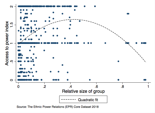
((a)) High degree of openness

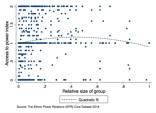
((b)) Low degree of openness

The figures plot a measure of the size of each ethnic group on the x-axis against each group’s access to power score on the y-axis, by historical level of political openness (i.e. PolityIV’s measure of Openness of Executive Recruitment, computed since 1800). Each point represents a group over a 10-year period. Figure (a) includes countries with an above-median level of historical political openness, and Figure (b) includes countries with a below-median level of historical political openness.

Figure III: Relative size and access to central power by level of political competitiveness

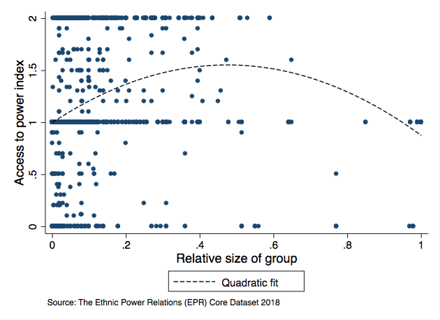
((a)) High degree of competitiveness

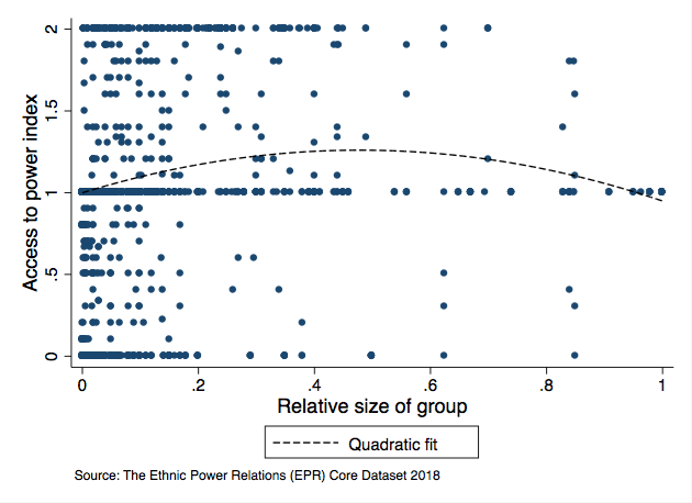
((b)) Low degree of competitiveness

The figures plot a measure of the size of each ethnic group on the x-axis against each group’s access to power score on the y-axis, by historical level of political competitiveness (i.e. PolityIV’s measure of Competitiveness of Executive Recruitment, computed since 1800). Each point represents a group over a 10-year period. Figure (a) includes countries with an above-median level of historical political competitiveness, and Figure (b) includes countries with a below-median level of historical political competitiveness.

Panel B: By competitiveness of executive recruitment       High degree of competitiveness       Low degree of competitiveness         (avg. xrcomp above median)       (avg. xrcomp below median)    Relative size 2.334^∗∗∗ 2.334^∗∗∗ 1.102^∗∗ 1.104^∗∗ 0.236^∗∗ (0.501) (0.502) (0.432) (0.432) (0.098) Relative size squared -2.458^∗∗∗ -2.458^∗∗∗ -1.150^∗∗ -1.151^∗∗ (0.514) (0.515) (0.463) (0.462) Joint significance 0.000 0.000 0.032 0.031 Vertex 0.475 0.475 0.479 0.480 R-squared 0.114 0.116 0.045 0.048 0.029 Observations 513227 513227 323235 323235 323235 Country fixed effects Y Y Y Y Y Period fixed effects Y Y Y Y Y Country/period fixed effects Y Y Y Y Y Group fixed effects N Y N Y Y    Notes: All columns report OLS estimates for estimates from Eq (1). The dependent variable in all columns is each ethnic group’s access to power score (as defined in Table I). The sample is limited to groups with a score of 2 or less, and the index is averaged over a 10-year period. In this subsample, the average relative size is 0.117 (with s.d. 0.224) and the average level of access to central power is 1.036 (with s.d. 0.575). Columns (1) and (2) in Panel A include countries with an above-median level of historical political openness, and Columns (3) to (5) in Panel A include countries with a below-median level of historical political openness (i.e. PolityIV’s measure of Openness of Executive Recruitment, computed since 1800). Columns (1) and (2) in Panel B include countries with an above-median level of historical political competitiveness, and Columns (3) to (5) in Panel B include countries with a below-median level of historical political competitiveness (i.e. PolityIV’s measure of Competitiveness of Executive Recruitment, computed since 1800). Robust standard errors clustered by country are in parentheses. $\dagger$ denotes results are statistically significant at the 15% level, * at the 10% level, ** at the 5% level, and *** at the 1% level.

Panel B: By competitiveness of executive recruitment     High compet.     Low compet.     High compet.     Low compet.   Relative size 2.334^∗∗∗ 1.172^∗∗∗ 0.250^∗∗ 2.333^∗∗∗ 1.165^∗∗∗ 0.245^∗∗ (0.511) (0.439) (0.105) (0.517) (0.442) (0.105) Relative size squared -2.448^∗∗∗ -1.229^∗∗ -2.448^∗∗∗ -1.226^∗∗∗ (0.524) (0.469) (0.530) (0.473) Joint significance 0.000 0.029 0.000 0.029 Vertex 0.477 0.477 0.477 0.475 R-squared 0.115 0.046 0.025 0.108 0.038 0.016 Observations 512876 322822 322822 512876 322822 322822 Country/period fixed effects Y Y Y Y N Y Group fixed effects N N Y Y N N Group-specific linear trends N N N Y N N   Notes: All columns report OLS estimates for estimates from Eq (1). The dependent variable in all columns is each ethnic group’s access to power score (as defined in Table I). The sample is limited to groups with a score of 2 or less, and the index is averaged over a 10-year period. In this subsample, the average relative size is 0.117 (with s.d. 0.224) and the average level of access to central power is 1.036 (with s.d. 0.575). Columns (1) and (2) in Panel A include countries with an above-median level of historical political openness, and Columns (3) to (5) in Panel A include countries with a below-median level of historical political openness (i.e. PolityIV’s measure of Openness of Executive Recruitment, computed since 1800). Columns (1) and (2) in Panel B include countries with an above-median level of historical political competitiveness, and Columns (3) to (5) in Panel B include countries with a below-median level of historical political competitiveness (i.e. PolityIV’s measure of Competitiveness of Executive Recruitment, computed since 1800). Robust standard errors clustered by country are in parentheses. $\dagger$ denotes results are statistically significant at the 15% level, * at the 10% level, ** at the 5% level, and *** at the 1% level.

Appendix: Proofs

Proof of Proposition 1.

I show that the relationship between the chance that (8) is satisfied and $\delta$ follows an inverted-U pattern. First, I define the function $f(\delta)$ as

$$f(\delta)=1-\frac{(1-\delta+a_{1})}{(1+a_{1})}\frac{(1-\lambda\delta)}{(1-\delta)}.$$ (11)

Note that (8) is satisfied if and only if $f(\delta)>0$. Thus, to show that the chance that $f(\delta)>0$ is satisfied follows an inverted-U pattern, I do the following: i) I show that there exists a $\delta^{*}\in(0,1)$ such that $f(\delta)$ is strictly increasing for all $\delta<\delta^{*}$, and strictly decreasing for all $\delta>\delta^{*}$; ii) I show that $f(\delta)>0$ for intermediate values of $\delta$, and $f(\delta)\leq 0$ for sufficiently small or large values of $\delta$. Figure 4 illustrates the function $f(\delta)$.

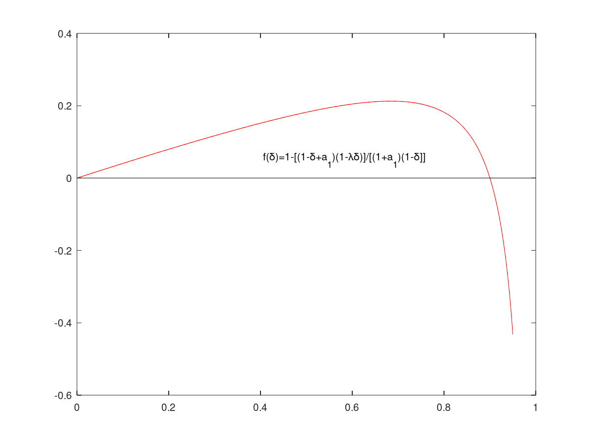
Figure 4: Parameters and outcomes ($\lambda=0.5$, $a_{1}=0.1$)

Note that $f(\delta)$ is differentiable within the interval $(0,1)$. Thus, differentiating $f(\delta)$ with respect to $\delta$, and rearranging, we have that

$$f^{\prime}(\delta)=-\frac{1}{(1+a_{1})}\Bigg{(}\frac{a_{1}-\lambda(1+a_{1})+2\lambda\delta-\lambda\delta^{2}}{(1-\delta)^{2}}\Bigg{)}.$$ (12)

Differentiating again and rearranging, we get

$$f^{\prime\prime}(\delta)=-\frac{2a_{1}(1-\lambda)}{(1+a_{1})(1-\delta)^{3}}.$$ (13)

From the last expression, note that for $\lambda,\delta\in(0,1)$ and $a_{1}>0$, $f^{\prime\prime}(\delta)<0$, which implies that $f(\delta)$ is strictly concave within the interval $(0,1)$. Thus, $f(\delta)$ has a unique global maximum in this interval. Let $\delta^{*}$ be this maximum, and note that since $f(\delta)$ is strictly concave, $\delta^{*}$ is determined by the first-order condition $f^{\prime}(\delta^{*})=0$, i.e., by

$$-\frac{1}{(1+a_{1})}\Bigg{(}\frac{a_{1}-\lambda(1+a_{1})+2\lambda\delta^{*}-\lambda(\delta^{*})^{2}}{(1-\delta^{*})^{2}}\Bigg{)}=0$$ (14)

which is satisfied if and only if

$$\lambda(\delta^{*})^{2}-2\lambda\delta^{*}-a_{1}+\lambda(1+a_{1})=0.$$ (15)

Now note that there is a unique $\delta^{*}\leq 1$ that solves the last equation. It is easy to see that $\delta^{*}$ is given by

$$\delta^{*}=1-\frac{\sqrt{a_{1}\lambda(1-\lambda)}}{\lambda}.$$ (16)

Finally, note that $\delta^{*}>0$ when

$$\ThisStyle{\lambda\mathord{\stretchto{\raisebox{2.3pt}{$\SavedStyle/$}}{}}(1-\lambda)}>a_{1}$$ (17)

which I assume in (6). Thus, there is a unique $\delta^{*}\in(0,1)$ such that $f(\delta)$ is increasing for all $\delta\in(0,\delta^{*})$ and decreasing for all $\delta\in(\delta^{*},1)$. This implies that $f(\delta)$ follows an inverted-U pattern within the interval $(0,1)$. To verify that $f(\delta)>0$ for intermediate values of $\delta$, first note that $f(\delta)$ crosses the x-axis twice within the interval $[0,1)$. To see this, note that $f(\delta)=0$ when

$$1-\frac{(1-\delta+a_{1})}{(1+a_{1})}\frac{(1-\lambda\delta)}{(1-\delta)}=0$$ (18)

which, rearranging, is equivalent to

$$\delta\big{(}a_{1}-(1+a_{1})\lambda+\lambda\delta\big{)}=0.$$ (19)

From the last expression, note that there are two different values for $\delta$, which I denote by $\underline{\delta}$ and $\overline{\delta}$, such that $f(\underline{\delta})=f(\overline{\delta})=0$ and $0\leq\underline{\delta}<\overline{\delta}<1$. In particular, note that $\underline{\delta}=0$ and $\overline{\delta}=1-\ThisStyle{a_{1}(1-\lambda)\mathord{\stretchto{\raisebox{2.3pt}{$\SavedStyle/$}}{}}\lambda}$, and that $\underline{\delta}<\overline{\delta}$ holds because of assumption (6). Given that $f(\delta)$ is strictly concave, this implies that $f(\delta)>0$ for all $\delta\in(\underline{\delta},\overline{\delta})$, which shows that $f(\delta)>0$ for intermediate values of $\delta$.

Finally, to see that $f(\delta)\leq 0$ for $\delta$ sufficiently small or sufficiently big, first note that $f(0)=0$. As for the case in which $\delta$ is sufficiently big, note that $f(\delta)<0$ for all $\delta\in(\overline{\delta},1)$.

∎

Proof of Proposition 2.

I follow the proof or Prop. 1. First, I define the function $h(\delta)$ as

$$h(\delta)=\gamma+\frac{(1-\gamma)}{(1-\delta)}-\frac{(1-\delta+a_{1})}{(1+a_{1})}\frac{(1-\lambda\delta)}{(1-\delta)}.$$ (20)

Note that (10) is satisfied if and only if $h(\delta)>0$. The purpose of the proof is to show that there is a $\gamma*\in[0,1]$ such that for all $\gamma>\gamma*$, Prop. 1 applies, and for all $\gamma<\gamma*$, the function $h(\delta)$ is strictly convex, strictly increasing and crosses the x-axis at $\delta=0$. This implies that when $\gamma<\gamma*$ (i.e. when political institutions are sufficiently persistent), the larger the relative size of a group, the more likely it is that the group will be given access to power. Figure 5 is the same as Figure 4, but with different values of $\gamma$. It also helps to understand what motivates Prop. 2: as $\gamma$ decreases, it becomes more likely that group 2 is given access to power when $\delta$ s sufficiently big.

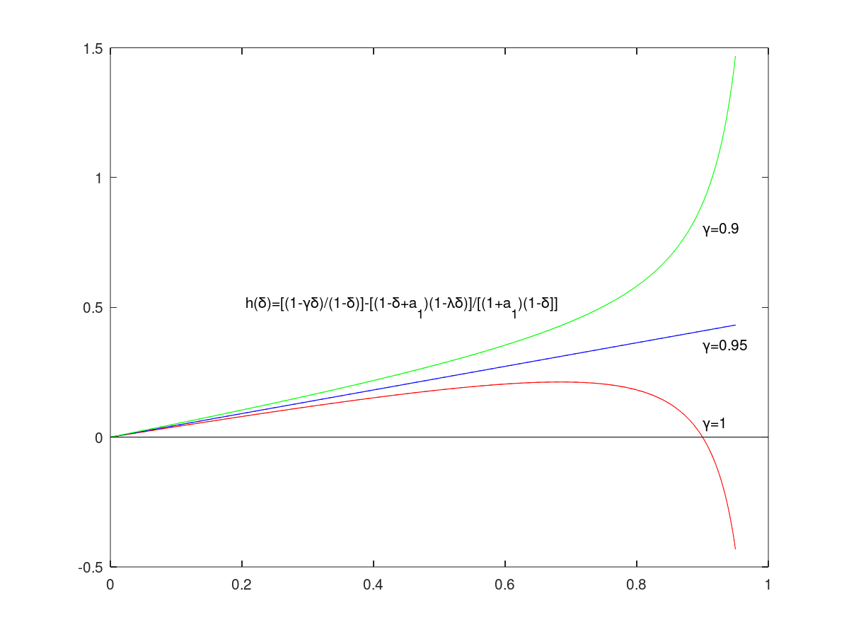
Figure 5: Parameters and outcomes ($\lambda=0.5$, $a_{1}=0.1$)

Repeating the analysis in the proof of Prop. 1, note that $h(\delta)$ is differentiable within the interval $(0,1)$. Thus, differentiating $h(\delta)$ with respect to $\delta$, and rearranging, we have that

$$h^{\prime}(\delta)=\frac{1}{(1-\delta)^{2}}\Bigg{[}(1-\gamma)-\frac{1}{(1+a_{1})}\big{(}a_{1}-\lambda(1+a_{1})+2\lambda\delta-\lambda\delta^{2}\big{)}\Bigg{]}.$$ (21)

Differentiating again, and rearranging, we get

$$h^{\prime\prime}(\delta)=\frac{2}{(1-\delta)^{3}}\Bigg{[}(1-\gamma)-\frac{a_{1}(1-\lambda)}{(1+a_{1})}\Bigg{]}.$$ (22)

Importantly, note that $h^{\prime\prime}(\delta)\gtrless$ for $\delta\in(0,1)$ if and only if

$$\frac{1+\lambda a_{1}}{(1+a_{1})}\lessgtr\gamma.$$ (23)

Now define $\gamma*=\frac{1+\lambda a_{1}}{(1+a_{1})}$, and note that $h^{\prime\prime}(\delta)<0$ for all $\gamma>\gamma*$ (i.e. $h(\delta)$ is strictly concave), and $h^{\prime\prime}(\delta)>0$ for all $\gamma<\gamma*$ (i.e. $h(\delta)$ is strictly convex).

Finally, I show that $h(\delta)$ is strictly increasing for all $\gamma<\gamma^{*}$ (and when $\delta\in(0,1)$). To see this, note from (21) that the condition $h^{\prime}(\delta)>0$ is equivalent to

$$\frac{(1+a_{1}\lambda)}{(1+a_{1})}+\frac{\lambda(1-\delta)^{2}}{(1+a_{1})}>\gamma.$$ (24)

And given the definition of $\gamma*$, the last condition is equivalent to

$$\gamma^{*}+\frac{\lambda(1-\delta)^{2}}{(1+a_{1})}>\gamma.$$ (25)

Thus, for all $\gamma<\gamma^{*}$, the last condition is satisfied.

Finally, note that $h(0)=0$, and

$$h^{\prime}(0)=1-\gamma+\lambda-\frac{a_{1}}{(1+a_{1})}$$ (26)

which is strictly positive given (6). This implies that $h(\delta)>0$ for all $\delta\in(0,1)$. So, when $\gamma$ is sufficiently small (such that $\gamma<\gamma*$), we have that $h(\delta)$ is strictly increasing, strictly convex, and $h(\delta)>0$. This shows that when institutions are sufficiently undemocratic, there is no longer an inverted-U-shaped relationship between a group’s relative size and its access to power.

∎

References

- (1)
- Acemoglu and Robinson (2008) Acemoglu, Daron and James A. Robinson, “Persistence of Power, Elites, and Institutions,” American Economic Review, March 2008, 98 (1), 267–93.
- Acemoglu et al. (2001) , Simon Johnson, and James A. Robinson, “The Colonial Origins of Comparative Development: An Empirical Investigation,” American Economic Review, December 2001, 91 (5), 1369–1401.
- Acemoglu et al. (2002) , , and , “Reversal of Fortune: Geography and Institutions in the Making of the Modern World Income Distribution*,” The Quarterly Journal of Economics, 11 2002, 117 (4), 1231–1294.
- Alesina and La Ferrara (2005) Alesina, Alberto and Eliana La Ferrara, “Ethnic Diversity and Economic Performance,” Journal of Economic Literature, September 2005, 43 (3), 762–800.
- Alesina et al. (2003) , Arnaud Devleeschauwer, William Easterly, Sergio Kurlat, and Romain Wacziarg, “Fractionalization,” Journal of Economic Growth, Jun 2003, 8 (2), 155–194.
- Alesina et al. (1999) , Reza Baqir, and William Easterly, “Public Goods And Ethnic Divisions,” The Quarterly Journal of Economics, November 1999, 114 (4), 1243–1284.
- Algan and Cahuc (2010) Algan, Yann and Pierre Cahuc, “Inherited Trust and Growth,” American Economic Review, December 2010, 100 (5), 2060–92.
- Allport (1954) Allport, G. W, The nature of prejudice, Reading, MA: Addison-Wesley, 1954.
- Banerjee and Iyer (2005) Banerjee, Abhijit and Lakshmi Iyer, “History, Institutions, and Economic Performance: The Legacy of Colonial Land Tenure Systems in India,” American Economic Review, September 2005, 95 (4), 1190–1213.
- Besley and Mueller (2018) Besley, Timothy and Hannes Mueller, Cohesive Institutions and the Distribution of Political Rents: Theory and Evidence, Cham: Springer International Publishing,
- Blalock (1967) Blalock, Hubert M., Toward a Theory of Minority-group Relations, New York: John Wiley and Sons, 1967.
- Blavatskyy (2010) Blavatskyy, Pavlo R., “Contest success function with the possibility of a draw: Axiomatization,” Journal of Mathematical Economics, 2010, 46.
- Blumer (1958) Blumer, Herbert, “Race Prejudice as a Sense of Group Position,” The Pacific Sociological Review, 1958, 1 (1), 3–7.
- Corchon and Dahm (2010) Corchon, Luis and Matthias Dahm, “Foundations for contest success functions,” Economic Theory, 04 2010, 43.
- Eeckhout (2006) Eeckhout, Jan, “Minorities and Endogenous Segregation,” The Review of Economic Studies, 2006, 73 (1), 31–53.
- Fearon (2003) Fearon, James D., “Ethnic and Cultural Diversity by Country*,” Journal of Economic Growth, Jun 2003, 8 (2), 195–222.
- Hirshleifer (1989) Hirshleifer, Jack, “Conflict and rent-seeking success functions: Ratio vs. difference models of relative success,” Public Choice, 11 1989, 63.
- Jia (2012) Jia, Hao, “Contests with the Probability of a Draw: A Stochastic Foundation*,” Economic Record, 2012, 88 (282), 391–406.
- Laitin and Jeon (2015) Laitin, David D. and Sangick Jeon, Exploring Opportunities in Cultural Diversity, American Cancer Society,
- Marshall and Jaggers (2019) Marshall, Monty G. and Keith Jaggers, “POLITY IV Project: Political Regime Characteristics and Transitions, 1800-2018,” Report, Center for Systemic Peace 2019.
- Moro and Norman (2004) Moro, Andrea and Peter Norman, “A general equilibrium model of statistical discrimination,” Journal of Economic Theory, 2004, 114 (1), 1 – 30.
- Oliver and Wong (2003) Oliver, Eric J. and Janelle Wong, “Intergroup Prejudice in Multiethnic Settings,” American Journal of Political Science, 2003, 47 (4), 567–582.
- Patsiurko et al. (2012) Patsiurko, Natalka, John L. Campbell, and John A. Hall, “Measuring cultural diversity: ethnic, linguistic and religious fractionalization in the OECD,” Ethnic and Racial Studies, 2012, 35 (2), 195–217.
- Pettigrew (1998) Pettigrew, Thomas F., “INTERGROUP CONTACT THEORY,” Annual Review of Psychology, 1998, 49 (1), 65–85. PMID: 15012467.
- Reed (2015) Reed, William Robert, “On the Practice of Lagging Variables to Avoid Simultaneity,” Oxford Bulletin of Economics and Statistics, 2015, 77 (6), 897–905.
- Schlueter and Scheepers (2010) Schlueter, Elmar and Peer Scheepers, “The relationship between outgroup size and anti-outgroup attitudes: A theoretical synthesis and empirical test of group threat- and intergroup contact theory,” Social Science Research, 2010, 39 (2), 285 – 295.
- Vogt et al. (2015) Vogt, Manuel, Nils-Christian Bormann, Seraina Ruegger, Lars-Erik Cederman, Philipp Hunziker, and Luc Girardin, “Integrating Data on Ethnicity, Geography, and Conflict: The Ethnic Power Relations Data Set Family,” Journal of Conflict Resolution, 2015, 59 (7), 1327–1342.