Higher Elastica: geodesics in the Jet Space

Abstract.

Carnot groups are subRiemannian manifolds. As such they admit geodesic flows, which are left-invariant Hamiltonian flows on their cotangent bundles. Some of these flows are integrable. Some are not. The space of k-jets for real-valued functions on the real line forms a Carnot group of dimension $k+2$. We show that its geodesic flow is integrable and that its geodesics generalize Euler’s elastica, with the case $k=2$ corresponding to the elastica, as shown in [1].

1. Introduction

The space of k-jets of real functions of a single real variable, denoted here by $\mathcal{J}^{k}$, is a $k+2$-dimensional manifold endowed with a canonical rank 2 distribution, by which we mean a linear sub-bundle of its tangent bundle. This distribution is framed by two vector fields, denoted $X_{1},X_{2}$ below, whose iterated Lie brackets give $\mathcal{J}^{k}$ the structure of a Carnot group. Declaring $X_{1}$ and $X_{2}$ to be orthonormal endows $\mathcal{J}^{k}$ with the structure of a subRiemannian manifold, one which is (left-) invariant under the Carnot group multiplication. Like any subRiemannian structure, the cotangent bundle $T^{*}\mathcal{J}^{k}$ is endowed with a Hamiltonian system whose underlying Hamiltionian $H$ is that whose solution curves project to the subRiemannian geodesics on $\mathcal{J}^{k}$. We call this Hamiltonian system the geodesic flow on $\mathcal{J}^{k}$.

Theorem 1.1.

The geodesic flow for the subRiemannian structure on $\mathcal{J}^{k}$ is integrable.

$\mathcal{J}^{1}$ is isometric to the Heisenberg group where this theorem is well-known see [2] and [3]. $\mathcal{J}^{2}$ is isometric to the Engel group and Ardentov and Sachkov showed that its subRiemannian geodesics correspond to Euler elastica. Their result inspired our next theorem.

$\mathcal{J}^{k}$ comes with a projection $\Pi:\mathcal{J}^{k}\to\mathbb{R}^{2}=\mathbb{R}^{2}_{x,u_{k}}$ onto the Euclidean plane which projects the frame $X_{1},X_{2}$ projects onto the standard coordinate frame ${{\partial}\over{\partial x}},{{\partial}\over{\partial u_{k}}}$ of $\mathbb{R}^{2}$. (See SETUP below for the meaning of the coordinates.) As a consequence, a horizontal curve $\gamma$ in $\mathcal{J}^{k}$ is parameteried by (subRiemannian ) arclength if and only if its planar projection $\Pi\circ\gamma$ to $\mathbb{R}^{2}$ is parameterized by arclength. We will characterize geodesics on $\mathcal{J}^{k}$ in terms of their planar projections. As alluded to already, Ardentov and Sachkov, [1], proved that when $k=2$ the planar projections of geodesics are Euler elastica. These elastica have “‘directrix” the $u_{2}$-line, the line orthogonal to the $x$-axis. There are many ways to characterize Euler’s elastica, see [4], [5] and [6], [7]. The one we will use is as follows. 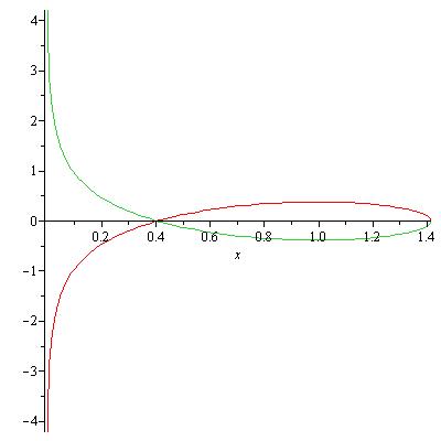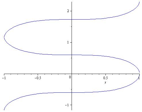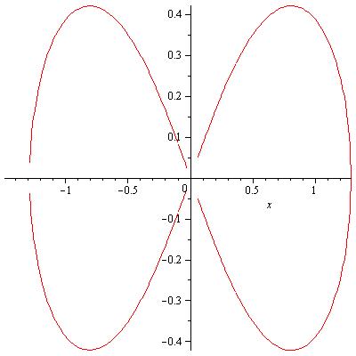Take a planar curve $c(s)=(x(s),y(s))$ and consider its curvature $\kappa=\kappa(s)$, where $s$ is arclength. Then the curve $c$ is an Euler elastica with directrix a line parallel to the y-axis if and only if $\kappa(s))=P(x(s))$ for $P(x)$ some linear polynomial in $x$ – that is $P(x)=ax+b$ for some constants $a$ and $b$. 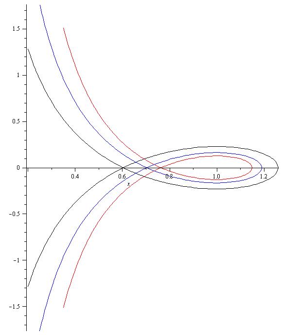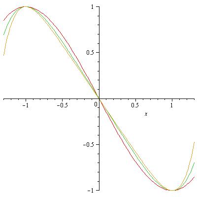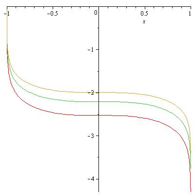See FIGURE 1.1.

Figure 1.1. Some clasic solutions of the Elastica equation generated by $F_{2}(x)=\frac{x^{2}}{a^{2}}-\alpha$, on the left the convict curve $\alpha=1$, in the center the pseudo-sinusoid $\alpha=0$ and on the left the pseudo-lemniscate with $\alpha=.65222...$.

Theorem 1.2.

Let $\gamma:I\to\mathcal{J}^{k}$ be a subRiemannian geodesic parameterized by arclength $s$ and $\pi\circ\gamma=c(s)=(x(s),u_{k}(s))$ its planar projection. Let $\kappa$ be the curvature of $c$. Then $\kappa(s)=p(x(s))$ for some degree $k-1$-polynomial $p(x)$ in the coordinate $x$. Conversely, any plane curve $c(s)$ in the $(x,u_{k})$ plane which is parameterized by arclength $s$ and whose curvature $\kappa(s)$ equals $p(x(s))$ for some polynomial $p(x)$ of degree at most $k-1$ in $x$ is the projection of such a subRiemannian geodesic.

Example For the case $k=1$ of the Heisenberg group the theorem asserts that $\kappa=P(x)$ where $P$ a degree $0$ polynomial – i.e. a constant function. The only curves having constant curvature are lines and circles, and these are well-known to be the projections of the Heisenberg geodesics.

2. set-up

The k-jet of a smooth function $f:\mathbb{R}\to\mathbb{R}$ at a point $x_{0}\in\mathbb{R}$ is its kth order Taylor expansion at $x_{0}$. We will encode this k-jet as a $k+2$-tuple of real numbers as follows:

(2.1) $$(j^{k}f)(x_{0})=(x_{0},f^{k}(x_{0}),f^{k-1}(x_{0}),\dots,f^{\prime}(x),f(x_{0}))\in\mathbb{R}^{k+2}$$

As $f$ varies over smooth functions and $x_{0}$ varies over $\mathbb{R}$, these $k$-jets sweep out the $k$-jet space, denoted by $\mathcal{J}^{k}$. $\mathcal{J}^{k}$ is diffeomorphic to $\mathbb{R}^{k+2}$ and its points are coordinatized according to

$$(x,u_{k},u_{k-1},\dots,u_{1},y)\in\mathbb{R}^{k+2}:=\mathcal{J}^{k}.$$

Recall that if $y=f(x)$ then $u_{1}=dy/dx$ while $u_{j+1}=du_{j}/dx$, $j\geq 1$. Rearranging these equations into $dy=u_{1}dx,du_{j}=u_{j+1}dx$ we see that $\mathcal{J}^{k}$ is endowed with a natural rank 2 distribution $\mathcal{D}\subset T\mathcal{J}^{k}$ characterized by the $k$ Pfaffian equations

$$u_{1}dx-dy = 0$$

$$u_{2}dx-du_{1} = 0$$

$$\vdots = \vdots$$

$$u_{k}dx-du_{k-1} = 0$$

The typical integral curves of $\mathcal{D}$ are the k-jet curves $x\mapsto(j^{k}f)(x)$. In addition to these integral curves we have a distinguished family of curves which arise by varying only the highest derivative $u_{k}$, and which are the integral curves of the vector field $X_{2}$ below (eq (2.2). These latter curves are $C^{1}$-rigid in the sense of Bryant-Hsu,[8], and they exhaust the supply of $C^{1}$-rigid curves.

A subRiemannian structure on a manifold consists of a non-integrable distribution together with a smoothly varying family of inner products on the distribution. We have our distribution $\mathcal{D}$ on $\mathcal{J}^{k}$. We arrive at our subRiemannian structure by observing that $\mathcal{D}$ is globally framed by the two vector fields

(2.2) $$X_{1}=\frac{\partial}{\partial x}+u_{1}\frac{\partial}{\partial y}+\sum_{i=2}^{k}u_{i}\frac{\partial}{\partial u_{i-1}}\;\;\text{and}\;\;X_{2}=\frac{\partial}{\partial u_{k}}$$

and then declaring these two vector fields to be orthonormal . Now the restrictions of the one-forms $dx,du_{k}$ to $\mathcal{D}$ form a global co-frame for $\mathcal{D}^{*}$ which is dual to our frame (eq (2.2). It follows that an equivalent way to describe our subRiemannian structure is to say that its metric is $dx^{2}+du_{k}^{2}$ restricted to $\mathcal{D}$.

For the purposes of theorem 1.2 the following alternative characterization of the subRiemannian metric is crucial. Consider the projection

$$\Pi:\mathcal{J}^{k}\to\mathbb{R}^{2}_{x,u_{k}};\Pi(x,u_{k},u_{k-1},\dots,u_{1},y)=(x,u_{k}).$$

Its fibers are transverse to $\mathcal{D}$ and we have that $\Pi_{*}X_{1}={{\partial}\over{\partial x}},\Pi_{*}X_{2}={{\partial}\over{\partial u_{k}}}$, so our frame pushes down to the standard frame for $\mathbb{R}^{2}$ The metric on each two-plane $\mathcal{D}_{p}$, $p\in\mathcal{J}^{k}$ is characterized by the condition that $d\Pi_{p}$ (which is just $\Pi$ since $\Pi$ is linear), restricted to $\mathcal{D}_{p}$ is a linear isometry onto $\mathbb{R}^{2}$, where $\mathbb{R}^{2}$ is endowed with the standard metric $dx^{2}+du_{k}^{2}$. It follows immediately that the length of any horizontal path equals the length of its planar projection, that $\Pi$ is a “submetry”: $\Pi(B_{r}(p))=B_{r}(\Pi(p))$, where $B_{r}(p)$ denotes the metric ball of radius $r$ about $q$, and that the horizontal lift a Euclidean line in $\mathbb{R}^{2}$ is a geodesic in $\mathcal{J}^{k}$.

2.1. Hamiltonian

Let $P_{1},P_{2}:T^{*}\mathcal{J}^{k}\to\mathbb{R}$ be the ‘power functions’ of the vector fields $X_{1},X_{2}$ above. (REF: [3], 8 pg.) . In terms of traditional cotangent coordinates $(x,u_{k},u_{k-1},\ldots,u_{1},y,p_{x},p_{k},p_{k-1},\ldots,p_{1},p_{y})$ for $T^{*}\mathcal{J}^{k}$, with $p_{i}$ short for $p_{u_{i}}$ we have

$$P_{1}=p_{x}+u_{1}p_{y}+u_{2}p_{1}+\ldots+u_{k}p_{k-1};\qquad P_{2}=p_{k}.$$

Then the Hamiltonian governing the subRiemannian geodesic flow on $\mathcal{J}^{k}$ is

(2.3) $$H=\frac{1}{2}(P_{1}^{2}+P_{2}^{2}).$$

See [3]; 8 pg. If we want our geodesics to be parameterized by arclength then we set $H=1/2$, and this we will do in what follows.

Remark. [$C^{1}$-rigidity.] The $u_{k}$ curves are $C^{1}$-rigid for $\mathcal{D}$, and form what Liu-Sussmann christened as the “regular-singular” curves for $\mathcal{D}$. As such, they are geodesics for any subRiemannian metric $Edx^{2}+2Fdxdu_{k}+Gdu_{k}^{2}$, restricted to $\mathcal{D}$. Such that $ds^{2}$ is positive definite, for $E,F,G$ any functions of the jet coordinates $(x,u_{k},u_{k-1},\ldots,y)$, regardless of whether or not they satsify the corresponding (normal) geodesic equations. For our metric each $u_{k}$-curve is indeed the projection to $\mathcal{J}^{k}$ of a solution to our $H$, so we do not go to extra effort to account for these abnormal geodesics. (REF [3], chapter 3).

3. Carnot Group structure

Under iterated bracket our frame $\{X_{1},X_{2}\}$ generates a $k+2$-dimensional nilpotent Lie algebra which can be identified pointwise with the tangent space to $\mathcal{J}^{k}$. Specifically, if we write

$$X_{3}=[X_{2},X_{1}],X_{4}=[X_{3},X_{1}],\ldots,X_{k+2}=[X_{k+1},X_{1}],0=[X_{k+2},X_{1}],$$

then we compute that

$$X_{k+2}={{\partial}\over{\partial y}},X_{k+1}={{\partial}\over{\partial u_{1}}},X_{k}={{\partial}\over{\partial u_{2}}},\ldots,X_{3}={{\partial}\over{\partial u_{k-1}}}$$

and that all other Lie brackets $[X_{i},X_{j}]$ are zero. The span of the $X_{i}$ thus form a $k+2$-dimensional graded nilpotent Lie algebra

$$\mathfrak{g}_{k}=V_{1}\oplus V_{2}\oplus\ldots V_{k+1},\;\;\;V_{1}=span\{X_{1},X_{2}\},V_{i}=span\{X_{i+1}\},1<i\leq k+1.$$

Like any graded nilpotent Lie algebra, this algebra has an associated Lie group which is a Carnot group $G$, and by using the flows of the $X_{i}$ we can identify $G$ with $\mathcal{J}^{k}$, and the $X^{i}$ with left-invariant vector fields on $G\cong\mathcal{J}^{k}$.

4. Integrability: Proof of theorem 1.1

.

Our Hamiltonian $H$ is a left-invariant Hamiltonian on the cotangent bundle of a Lie group $G$. We recall the general ‘Lie-Poisson” structure for such Hamiltonian flows. [9] Appendix; REF: local struc Poisson, [10] ch 4.

The arrows $J_{R},J_{L}$ are the momentum maps for the actions of $G$ on itself by right and left translation, lifted to $T^{*}G$. The subscripts $\pm$ are for a plus or minus sign in front of the Lie-Poisson (=Kostant-Kirrilov-Souriau) bracket on $\mathfrak{g}^{*}$. $J_{R}$ corresponds to left translation back to the identity and realizes the quotient of $T^{*}G$ by the left action. $J_{L}$ corresponds to right translation of a covector back to the identity and forms the components of the momentum map for left translation, lifted to the cotangent bundle. In our case, ${\mathfrak{g}^{*}}=\mathbb{R}^{k+2}$ and

$$J_{R}=(P_{1},P_{2},P_{3},\ldots,P_{k+2})$$

with $P_{i}$ the power function associated to $X_{i}$, so that

$$P_{3}=p_{k-1},P_{4}=p_{k-2},\ldots,P_{k+2}=p_{y}$$

in terms of standard canonical coordinates as above.

When the Hamiltonian $H:T^{*}G\to\mathbb{R}$ is left-invariant it can be expressed as a function of the components of $J_{R}$, that is $H=h\circ J_{R}$ for some $h:{\mathfrak{g}}^{*}\to\mathbb{R}$, and $H$ Poisson commutes with every component of the left momentum map $J_{L}$, so that these left-components are invariants. $J_{L}$ and $J_{R}$ are related by $J_{L}(g,p)=(Ad_{g})^{*}J_{R}(g,p)$ where we have written $p\in T_{g}^{*}G$ and where $Ad_{g}$ is the adjoint action of $g$.

The reason underlying the integrability of our system is a simple dimension count.

Proposition 4.1.

If the generic co-adjoint orbit of ${\mathfrak{g}}^{*}$ is 2-dimensional then the left-invariant Hamiltonian flow on $T^{*}G$ is integrable.

Recall that the symplectic reduced spaces for left translation action are the co-adjoint orbits, for ${\mathfrak{g}}^{*}_{+}$, and that $J_{R}$ realizes this symplectic reduction procedure, mapping each $J_{L}^{-1}(\mu)$ onto the co-adjoint orbit through $\mu$. The hypothesis of the Proposition asserts that the symplectic reduced spaces associated to the $G$-action are zero or two dimensional, so, morally speaking, the system is automatically integrable by reasons of dimension count.

Proof of Proposition. We must produce $n$ commuting integrals in involution, where $n=dim(G)$. The hypothesis asserts that there are $n-2$ Casimirs $C_{1},\ldots,C_{n-2}$ for ${\mathfrak{g}}^{*}$, these being the functions whose common level sets at a generic value define a generic co-adjoint orbit. These Casimirs are a functional basis for the $Ad^{*}_{G}$ invariant polynomails on ${\mathfrak{g}}^{*}$. When viewed as functions on $T^{*}G$ via $C_{i}\circ J_{R}$ the Casimirs Poisson commute with any left-invariant function on $T^{*}G$, and in particular with $H$ and with each other. Thus, $H,C_{1},C_{2},\ldots,C_{n-2}$ yield $n-1$ integrals. To get the last commuting integral take any component of $J_{L}$. QED.

Proof of theorem 1.1. In order to use the proposition, we need to verify that the co-adjoint orbits are generically 2-dimensional. We have the Poisson brackets

(4.1) $$\{P_{1},P_{i}\}=P_{i+1},1<i<k+1,\qquad\text{and}\qquad\{P_{1},P_{k+2}\}=0.$$

with all other Poisson brackets $\{P_{i},P_{j}\},1<i<j\leq k+2$ being zero. Thus the Poisson tensor $B$ at a point $Z=(P_{1},P_{2},P_{3},\ldots,P_{k+2})\in{\mathfrak{g}}^{*}_{+}$ is :

(4.2) $$B:=\begin{pmatrix}0&Z_{k}&0\\ Z_{k}^{t}&0&0\\ 0&0&0\\ \end{pmatrix}\;\;\text{where}\;\;Z_{k}=(P_{3},\ldots,P_{k+2}).$$

which has rank $2$ generically and rank $0$ if and only if $Z_{k}=0$, i.e. if and only if $P_{i}=0$ for $2<i$. QED

Thanks to this information we now that the system has $k$ Casimir functions.

Theorem 4.2.

If $P_{k+2}\neq 0$ the function $C_{i}(P_{2},P_{3},\ldots,P_{k+2})$, with $i\in\{1,\dots,k\}$ which are given by $C_{1}(P_{2},P_{3},\ldots,P_{k+2})=P_{k+2}$, and for $i>1$, we define as

(4.3) $$\begin{split}C_{i}=&\;P_{k+2}^{i-1}P_{k+2-i}+\sum_{j=1}^{i-2}(-1)^{j}P_{k+2}^{i-(j+1)}P_{k+2-j}\frac{P_{k+1}^{j}}{(j)!}+(-1)^{i-1}\frac{P_{k+1}^{i}}{(i-2)!\;i},\end{split}$$

are constant of motion for the geodesic equations in $\mathcal{J}^{k}$, in others words they are Casimir functions.

5. Integration and curvature: proof of theorem 1.2

Hamilton’s equations read $\frac{df}{dt}=\{f,H\}$. With our Hamiltonian they expand out to $\frac{df}{dt}=\{f,P_{1}\}P_{1}+\{f,P_{2}\}P_{2}$. Returning to our coordinates $x,u_{k}$ we compute $\{x,P_{1}\}=1,\{x,P_{2}\}=0$, $\{u_{k},P_{1}\}=0,\{u_{k},P_{2}\}=1$ so that

(5.1) $$\frac{dx}{dt}=P_{1}\qquad\text{and}\qquad\frac{du_{k}}{dt}=P_{2}.$$

Thus $(P_{1},P_{2})$ are the components of the tangent vector to the plane curve $(x(s),u_{k}(s))$ obtained by projecting a geodesic to the plane. If $H=1/2$ then this vector is a unit vector, the parameter $t$ of the flow is arc-length $s$ and we can write

$$(P_{1},P_{2},\dot{\theta})=(\cos(\theta),\sin(\theta),\kappa)$$

Using $\{P_{1},P_{2}\}=P_{3}$ we see that the $P_{1}$, evolve according to

(5.2) $$\begin{split}\dot{P}_{1}&=P_{3}P_{2}\\ \dot{P}_{2}&=-P_{3}P_{1}.\\ \end{split}$$

But we also have $\dot{P}_{1}=-\dot{\theta}\sin(\theta)=-\dot{\theta}P_{2}$ and $\dot{P}_{2}=+\dot{\theta}\cos(\theta)=+\dot{\theta}P_{1}$ from which we see that

$$-P_{3}=\kappa.$$

Now for $k+2>i>2$ we have that $\{P_{i},P_{1}\}=-P_{i+1},\{P_{i},P_{2}\}=0$, and $\{P_{j},P_{k+2}\}=0$ for all $j$ so that

(5.3) $$\begin{split}\dot{P}_{3}&=-P_{1}P_{4},\\ \dot{P}_{4}&=-P_{1}P_{5},\\ \vdots\\ \dot{P}_{k+1}&=-P_{1}P_{k+2},\\ \dot{P}_{k+2}&=0.\\ \end{split}$$

Proof of theorem 1.2. Consider a geodesic $\gamma$ and an arc of the geodeisc for which $\dot{x}\neq 0$. Instead of arclength $t=s$ use $x$ to parameterize this arc. From eq (5.1) we have, along this arc, that

$$\frac{d}{dx}=\frac{1}{P_{1}}\frac{d}{ds}$$

so that the equations for the evolution of $P_{3},P_{4},\ldots,P_{k+2}$ along the curve become

$$\frac{dP_{3}}{dx}=-P_{4}$$

$$\frac{dP_{4}}{dx}=-P_{5}$$

$$\ldots$$

$$\frac{dP_{k+1}}{dx}=-P_{k+2}$$

$$\frac{dP_{k+2}}{dx}=0$$

These equations can be summarized by

$$\frac{d^{k}P_{3}}{dx^{k}}=0$$

which asserts that the curvature $P_{3}$ of the projected curve $c=\pi\circ\gamma$, is a polynomial $p(x)$ of degree $k-1$ in $x$, at least along our arc. Finally, since $\gamma$ is an analytic function of $s$, so are $c(s)$ and $\kappa(s)$, so that if $\kappa(s)$ enjoys a relation $\kappa(s)=p(x(s))$ along some subarc of $c(s)$, it enjoys this same relation everywhere along $c$.

To prove the converse, first consider a general smooth curve in the $x-u$ plane along which $dx>0$. We can parameterize the curve either by arc-length $s\mapsto(x(s),u(s))$ or as graph, $u=u(x)$. Define the function $F(x)$, with $-1\leq F(x)\leq 1$ by way of relating the two parameterizations:

(5.4) $$(\dot{x},\dot{u}):=(\frac{dx}{ds},\frac{du}{ds})=(\sqrt{1-F(x)^{2}},F(x))$$

so that $dx=\sqrt{1-F(x)^{2}}ds$ and

$$u^{\prime}(x):=\frac{du}{dx}=\frac{F(x)}{\sqrt{1-F(x)^{2}}}$$

It follows that

$$u^{\prime\prime}=\frac{F^{\prime}}{(1-F(x)^{2})^{3/2}}.$$

Now the curvature of our curve, when viewed as a graph, is well known to be

$$\kappa(x)=\frac{u^{\prime\prime}(x)}{(1+u^{\prime}(x)^{2})^{3/2}}$$

and we have

$$(1+u^{\prime}(x)^{2})=\frac{1}{1-F(x)^{2}}$$

from which we conclude that

(5.5) $$\kappa=F^{\prime}(x).$$

To finish the proof, suppose that we are given a curve $c$ in the $x-u$ plane, with $u=u_{k}$, whose curvature $\kappa$ is a degree $k-1$ polynomial in $x$. Define $F(x)$ by eq (5.4) along an arc of $c$ for which $dx>0$ From eq (5.5) we know that $F$ is an anti-derivative of $\kappa$ and so a polynomial of degree $k$ in $x$. (The constant term in the integration $F(x)=\int^{x}\kappa dx$ is fixed by choosing any point $(x_{*},u_{*})=(x(s_{*}),u(s_{*}))$ along $c$ for which $dx/ds>0$ so that $-1<du/ds|_{s=s_{*}}<1$ and setting $F(x_{*})=du/ds|_{s=s_{*}}$.) By the preceding analysis, $c$ has curvature $\kappa(x(s))$ along the entire arc $dx>0$ of our curve which contains $(x_{*},u_{*})$. Moreover $u^{\prime}(x)=F(x)/\sqrt{1-F(x)^{2}}$. Set

(5.6) $$(P_{1}(x),P_{2}(x)):=(\sqrt{1-(F(x))^{2}},F(x)),,$$

(5.7) $$P_{3}(x):=F^{\prime}(x),\;\;\text{and}\;\;P_{i+2}:=(-1)^{i}\frac{d^{i}F}{d^{i}x}(x),i>1.$$

View the $P_{i}$ as momentum functions. Reparameterize the momentum functions by $s$ using $dx/ds=P_{1}(x)$. Then we verify that the $P_{i}$ satisfy 5.2 and 5.3, so that the horizontal curve $\gamma(x(s))$ in $\mathcal{J}^{k}$ with these momenta satisfies the geodesic equations and projects on our given curve $c$.

QED

Corollary 5.1.

Suppose that the momentum functions $P_{i}$ are related to the degree $k$ polynomial $F(x)$ as per equations (5.6, 5.7) and that $H=1/2$. Then a critical point $x_{0}$ of $F(x)$ corresponds to a relative equilibrium for the reduced equations 5.2 and 5.3 if and only if $F(x_{0})=\pm 1$.

Proof. The equilibria of equations (5.2) and (5.3) are the points with $P_{1}=0$ and $P_{3}=0$, as long as $H\neq 0$. If $H=\frac{1}{2}$, the condition $P_{1}=0$ forces $P_{2}=\pm 1$ but $P_{2}=F(x)$. Finally $P_{3}=F^{\prime}(x)$.

6. Structure of higher Elastica

As we see in the last prove we have an option to select a primitive of $p(x)$, then given $F_{k}(x)=\int p(x)dx$ the dynamics is trivial when $F_{k}^{-1}([-1,1])$ is empty or isolated points, i.e. $F_{(}x(s))$ is constant for all $s$. Then we can take $F_{k}^{-1}([-1,1])$ as follow

$$F_{k}^{-1}([-1,1]):=\cup_{I}[x_{0}^{i},x_{1}^{i}]\qquad\text{where}\qquad F_{k}(x^{i}_{0})=\pm 1,\quad F_{k}(x^{i}_{1})=\pm 1,$$

$x_{0}^{i}<x_{1}^{i}\leq x_{0}^{i+1}<x_{1}^{i+1}$ and the condition that $F_{k}(x)\neq\pm 1$ if $x\in(x_{0}^{i},x_{1}^{i})$, note all the possibilities. Choose $[x_{0}^{i},x_{1}^{i}]=[x_{0},x_{1}]$, by the last corollary the points $x_{0}$ and $x_{1}$ are equilibrium points if and only if they are critical points of the function $F_{k}(x)$, then it takes infinite time to arrive to them.

Theorem 6.1.

The curve $(x,u)$ with curvature $k((x(s))=p(x)$ is bounded in the $x$-direction, and generically the curve is periodic in $x$ and the period $L$ given by

$$L:=\int_{x_{0}}^{x_{1}}\frac{2dx}{\sqrt{1-F_{k}^{2}(x)}}\;\;\text{we also define }\;\;\tau=\int_{x_{0}}^{x_{1}}\frac{2F_{k}(x)dx}{\sqrt{1-F_{k}^{2}(x)}}.$$

Finally, we have that $u(s+L)=u(s)+\tau$.

Let $x_{0}$ be a regular point, we will answer the question how to extend the curve $c(s)$ as a function of $x$ such that its lift is a smooth solution of geodesics equation, set $(P_{1},P_{2})=(\cos\theta,\sin\theta)$ and $\dot{\theta}=p(x)$ since $F_{k}(x_{0})=\pm 1$ define $\theta(x_{0})=\pm\frac{\pi}{2}$ and $\dot{\theta}(x_{0})\neq 0$, then $P_{1}$ has a change of sign, while, $P_{2}$ does not change. Therefore if $x(s_{0})=x_{0}$ we define

(6.1) $$(\dot{x},\dot{u})=\begin{cases}(\pm\sqrt{1-F_{k}^{2}(x)},F_{k}(x))\qquad\text{if}\qquad s_{0}-\frac{L}{2}\leq s\leq s_{0},\\ (\mp\sqrt{1-F_{k}^{2}(x)},F_{k}(x))\qquad\text{if}\qquad s_{0}\leq s\leq s_{0}+\frac{L}{2}.\end{cases}$$

Therefore, the curve stays in the interval $[x_{0},x_{1}]$, same with $x_{1}$. If both are regular point, we can read the equation $P_{1}=\sqrt{1-F_{k}(x)}$ as the restriction $P_{1}(x)|_{\{H=\frac{1}{2},C_{1},\dots,C_{k}\}}$ and consider action function $I$ given by the area under the graph $\sqrt{1-F_{k}(x)}$ going from $x_{0}$ to $x_{1}$ and the area of $-\sqrt{1-F_{k}(x)}$ going from $x_{1}$ to $x_{0}$, i.e.

$$\mathcal{I}(H=\frac{1}{2},C_{1},\dots,C_{k}):=2\int_{x_{0}}^{x_{1}}\sqrt{1-F_{k}(x)}dx.$$

Finally, the period is given by $\frac{\partial\mathcal{I}}{\partial H}|_{\{H=\frac{1}{2},C_{1},\dots,C_{k}\}}=L$, (see [9] chapter 10). The period goes to infinite when $x_{0}$ or $x_{1}$ are critical points, much like the very well known homolinic connection of a pendulum.

Let us consider $(x_{0},u_{*})$ the initial point of the curve and $x(s)\in[x_{0},x_{1}]$ and $2s\leq L$, then

$$\begin{split}u(s)+\tau&=\int_{x_{0}}^{x(s)}\frac{F_{k}(x)dx}{\sqrt{1-F_{k}^{2}(x)}}+\int_{x_{0}}^{x_{1}}\frac{2F_{k}(x)dx}{\sqrt{1-F_{k}^{2}(x)}}+u_{*},\\ &=(\int_{x_{0}}^{x(s)}+\int_{x(s)}^{x_{1}}+\int_{x_{0}}^{x_{1}}+\int_{x_{0}}^{x(s+L)})\frac{F_{k}(x)dx}{\sqrt{1-F_{k}^{2}(x)}}+u_{*}=u(s+L).\\ \end{split}$$

Where again we use the fact that $\int_{x_{0}}^{x_{1}}\frac{F_{k}(x)dx}{\sqrt{1-F_{k}^{2}(x)}}=\int_{x_{1}}^{x_{0}}\frac{F_{k}(x)dx}{-\sqrt{1-F_{k}^{2}(x)}}$. QED

Here, we have three cases;

• Periodic case - $p(x_{0})\neq 0$ and $p(x_{1})\neq 0$

• Asymptotic behavior to one line - $p(x_{0})=0$ and $p(x_{1})\neq 0$ or $p(x_{0})\neq 0$ and $p(x_{1})=0$ .

• Asymptotic behavior to two line - $p(x_{0})=0$ and $p(x_{1})=0$ .

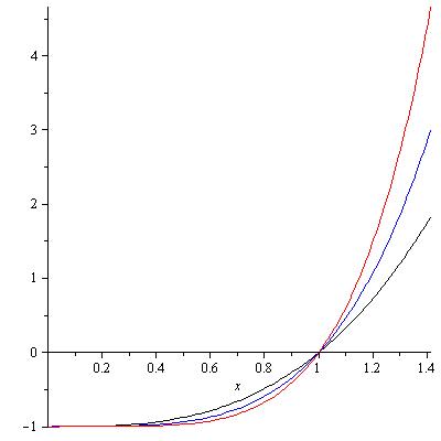
6.1. General Convict curve

The elastica equation has a distinguished solution which we call the Euler Kink. Other names for it are the Euler soliton or Convict’s curve. See figure and see 1.1, see [1], [6], [7] and [4]. We define the Convict’s curve at the level $k$ in the sense that the curvature of the curve $(x,u_{k}(x))$ it is always proportional to $x^{k-1}$. See figure 6.1

Theorem 6.2.

If $1<k$ then the level $k$ has a convict curve.

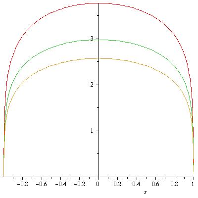
Figure 6.1. On the left side we see $F_{k}(x)$, while, on the right side we have the curves in the plane $(x,u)$ for $k=3,4,5$ .

Consider the polynomial $F_{k}(x)=\frac{x^{k}}{a^{k}}-\alpha$. Set $x=a\sqrt[k]{\alpha+\cos(t)}$ , we can find the next expressions

$$\begin{split}u(t)=\int_{t_{0}}^{t_{1}}\frac{\cos(t)dt}{(\alpha+\cos(t))^{\frac{k-1}{k}}},&\;\;\;t(x)=\frac{a}{k}\int_{t_{0}}^{t_{1}}\frac{dt}{(\alpha+\cos(t))^{\frac{k-1}{k}}}.\\ \end{split}$$

The case $k=2$ is the classic solution for Elastica equation, see [7] page 436. If $\alpha=1$, then we have the explicit expression

$$\begin{split}u(x)&=\int^{x}_{\sqrt[k]{2}}\frac{x^{\frac{k}{2}}dx}{\sqrt{2-x^{k}}}-\frac{2}{k\sqrt{2}}\ln(\frac{\sqrt{2}-\sqrt{2-x^{k}}}{x^{\frac{k}{2}}}),\\ t(x)&=\frac{1}{\frac{3}{2}\sqrt{2}}\ln(\frac{\sqrt{2}-\sqrt{2-x^{k}}}{x^{\frac{k}{2}}}).\\ \end{split}$$

We can find a explicit second order ODE for $\dot{\theta}$,

$$\begin{split}p_{u_{k-1}}=\frac{\partial P}{\partial x}(x)=kx^{k-1}\;\;\;\text{and}\;\;\;\frac{\dot{\theta}^{2}}{k^{2}a^{2k}}=(\cos\theta+\alpha)^{\frac{2(k-1)}{k}}.\\ \end{split}$$

In the case $k=2$ is the pendulum equation define in [1], the ODE equation can be extend to $k=1$. Also, $\alpha=1$ degenerate a system with a degenerated equilibrium point with a homoclinic connection.

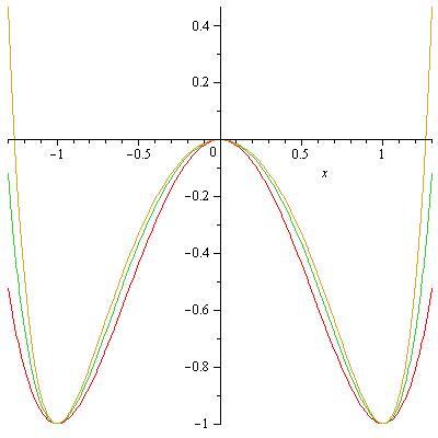
Figure 6.2. On the left side we see $F_{k}(x)$, while, on the right side we have the curves in the plane $(x,u)$ for $k=3,5,7$.

6.2. Infinite geodesic graph.

Here, we will define a infinite geodesic graph like the curve whose projection to the plane $(x,u)$ is always a graph of $x$. See figure 6.2 and 6.3.

Theorem 6.3.

If $k>2$ then $\mathcal{J}^{k}$ has a geodesic graph.

We split in the even and odd case:

Figure 6.3. On the left side we see $F_{k}(x)$, while, on the right side we have the curves in the plane $(x,u)$ for $k=4,6,8$.

• Consider the polynomial $F_{2k+1}(x)=-\frac{x^{2k+1}-(2k+1)x}{2k}$ with $x\in[-1,1]$. Since the point $x=\pm 1$ give us $F_{2k+1}(\pm 1)=\pm 1$ and $\frac{\partial F}{\partial x}(\pm 1)=0$ they are equilibrium points.

• Consider the polynomial $F_{2k}(x)=-\frac{x^{2k}-kx^{2}}{1-k}$, with $x\in[-1,1]$. Since the point $x=\pm 1$ give us $F_{2k}(\pm 1)=-1$, and $\frac{\partial F}{\partial x}(\pm 1)=0$.

QED