Variations of the physical parameters of the blazar Mrk 421 based on the analysis of the spectral energy distributions

Abstract

We report on the variations of the physical parameters of the jet observed in the blazar Mrk 421, and discuss the origin of X-ray flares in the jet, based on the analysis of the several spectral energy distributions (SEDs). The SEDs are modeled using the one-zone synchrotron self-Compton (SSC) model and its parameters determined using a Markov chain Monte Carlo method. The lack of data at TeV energies means many of the parameters cannot be uniquely determined and are correlated. These are studied in detail. We found that the optimal solution can be uniquely determined only when we apply a constraint to one of four parameters: the magnetic field ($B$), Doppler factor, size of the emitting region, and normalization factor of the electron energy distribution. We used 31 sets of SED from 2009 to 2014 with optical–UV data observed with UVOT/$\it{Swift}$ and the Kanata telescope, X-ray data with XRT/$\it{Swift}$, and $\gamma$-ray data with the $Fermi$ Large Area Telescope (LAT). The result of our SED analysis suggests that, in the X-ray faint state, the emission occurs in a relatively small area ($\sim 10^{16}\;{\rm cm}$) with relatively strong magnetic field ($B\sim 10^{-1}\;{\rm G}$). The X-ray bright state shows a tendency opposite to that of the faint state, that is, a large emitting area ($\sim 10^{18}\;{\rm cm}$), probably in the downstream of the jet and weak magnetic field ($B\sim 10^{-3}\;{\rm G}$). The high X-ray flux was due to an increase in the maximum energy of electrons. On the other hand, the presence of two kinds of emitting areas implies that the one-zone model is unsuitable to reproduce, at least a part of the observed SEDs.

1 Introduction

Blazars are a type of active galactic nuclei (AGN) whose jets are directed toward us. The radiation of the jet dominates the entire spectral energy distribution (SED) due to a strong beaming effect ([Urry, Padovani (1995)]). This effect also causes rapid variability and high luminosity, commonly observed in blazars. Hence, blazars are good candidates for studying the physical processes of relativistic jets.

The SED of blazars extends from the radio to the $\gamma$-ray bands ([Fossati et al. (1998)]). They exhibit two broad components: a low energy component, attributed to synchrotron radiation from relativistic electrons, and a high energy component, generally believed to be inverse Compton (IC) scattering by electrons. The local synchrotron radiation can act as seed photons for the IC process. This scenario is called the synchrotron self-Compton (SSC) process ([Tavecchio et al. (1998)]). The modeling of SED with a given radiation mechanism, like the SSC process, allows us to investigate the intrinsic physical properties of the emitting regions of the blazar and the physical conditions of the jet (e.g., [Ghisellini et al. (2009)]; [Böttcher (2007)]).

The SSC model can be expressed with about $10$ physical parameters, including the magnetic field, Doppler factor, and parameters of the electron energy distribution (e.g., [Finke et al. (2008)]). It is difficult to determine the unique solution of the problem because some of the parameters are strongly correlated and the model is degenerate. In previous studies, the parameters were estimated by fixing the size of the emitting region (e.g., [Bartoli et al. (2016)]), Doppler factor, magnetic field, or all of them (e.g., [Tramacere et al. (2009)]; [Itoh et al. (2015)]). The model optimization procedure is sometimes based on a “fit-by-eye” method, with which a real solution can be easily overlooked, in particular if the model is degenerate (e.g., [Böttcher et al. (2013)]).

The optimal solution may be misidentified if the parameters are set to unsuitable values. In evaluating the likelihood function or posterior probability density function in a multidimensional space, it is essential to understand the degenerate structure of the model and thereby to establish a method to estimate the optimal solution. The likelihood function also allows the uncertainty of the parameters to be estimated, which is especially important for considering the variations of the model parameters.

Mrk 421 ($z=0.031$) is a well-known nearby blazar ([Punch et al. (1992)]). It is a very active source, exhibiting major outbursts about once every two years composed of many short flares of both X-rays and $\gamma$-rays ([Aielli et al. (2010)]; [Bartoli et al. (2011)]). The SED of Mrk 421 can be modeled with a simple one-zone SSC model ([Paggi et al. (2009)]; [Abdo et al. (2011)]). Thus, Mrk 421 is an ideal object to study the variations of the SSC model parameters, and thereby to understand the physical process in the jets.

In this paper, we use the Markov chain Monte Carlo (MCMC) method to study the degenerate structure of the SSC model and a proper methodology for fitting the model to the SED data. Vianello et al. (2015) propose a method to estimate the model parameters not from the prepared SED data, but from the count-based data obtained with each instrument. Since the SED data is usually prepared through a fitting procedure to each count-based data, the method provides a better way to achieve the true maximum likelihood solution. The present paper focuses on the classical analysis with the SED data, whereas the degenerate structure of the model is common in both methods. We investigate the variation of the physical parameters of the jet using the SED data of Mrk 421 from 2009 to 2014, which includes a bright X-ray outburst in 2010. The paper is organized as follows. In Section 2 we introduce the dataset. In Section 3 we describe the model and MCMC method. We demonstrate that we need to restrict one parameter to uniquely determine the optimal solution. In this paper, we set two kinds of restrictions: on the size of the emitting region (or the variation time-scale), and on the Doppler factor. In Section 4 we report on a time-series analysis for the estimation of the variation time-scale of the object. The results of the SED analysis are presented in Section 5, followed by a discussion of the origin of the X-ray variation in Section 6. Section 7 is a summary.

2 Observations

2.1 X-ray data

The Neil Gehrels Swift observatory is a NASA mission, launched in 2004, devoted to observing fast transients, namely prompt and afterglow emission of $\gamma$-ray bursts (Gehrels et al., 2004). The satellite carries three sets of instruments: the Burst Alert Telescope (BAT; 15–150 keV; Gehrels et al. (2004)), the X-Ray Telescope (XRT; 0.3–10 keV; Burrows et al. (2005)), and the Ultra-Violet Optical Telescope (UVOT; 170–650 nm; Roming et al. (2005)). In this paper, we analyzed the data of Mrk 421 taken by $\it{Swift}$ between 2009 and 2014.

The $\it{Swift}$-XRT is a Wolter type-I grazing incidence telescope that focuses X-rays onto a CCD. This instrument has a 110 $\rm{cm}^{2}$ effective area, 23.6 arcmin FOV, and 15 arcsec angular resolution. The XRT data of Mrk 421 used in this paper were all taken in windowed timing mode, due to the high flux rate of the source. The exposure time of each run is typically $10^{3}\;{\rm s}$. The XRT data were reduced using the software distributed with the HEASoft v6.19 package by NASA High Energy Astrophysics Archive Research Center (HEASARC). Spectral analysis was performed with XSPEC version 12.9.0o. We fitted the XRT spectra with a log-parabolic or power-law shape component and the Galactic absorption component represented by the wabs model over an energy range of 0.3–10 keV. The column density of the absorbing component was fixed to $1.61\times 10^{20}\,{\rm cm}^{-2}$ (Lockman, Savage, 1995). We confirmed that the $\chi^{2}$ values for the power-law model were larger than those for the log-parabolic model for all data sets. The difference in $\chi^{2}$ was at least 3, and mostly $>50$. Examples of the X-ray spectra are shown in Figure 1. The residuals between the data and power-law model are systematically large both in $\lesssim 0.5$ keV and $\gtrsim 5$ keV, compared with those of the log-parabolic model. Hence, all data was analyzed with the log-parabolic model. In the SED fitting performed in Section 3 and 5, we use the absorption corrected XRT data.

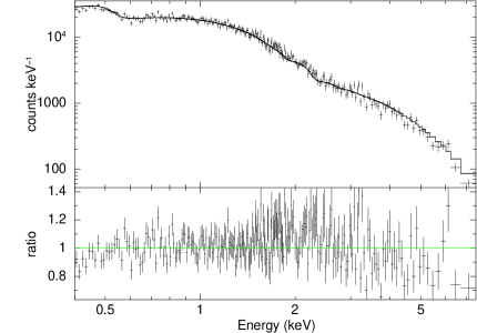
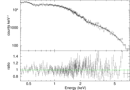
Figure 1: Examples of the X-ray spectra and models of Mrk 421. The data shown in the figure were taken by Swift/XRT on MJD 55186. For each panel, the ratio of the data to model is also shown. The power-law and log-parabolic models are used in the upper and lower panels, respectively.

Figure 2: X-ray light curve of Mrk 421 for 2009–2014 obtained with XRT/$\it{Swift}$. The gray line indicates the light curve of all data. The filled circles and triangles indicate the epochs at which we report the estimated SED parameters in this paper. The triangles show the epochs at which the optical and near-infrared Kanata observations are available. The open symbols indicate the epochs of the outlier SEDs (see section 3.3). The measurement error is smaller than the symbol size.

Figure 2 shows the X-ray light curve of Mrk 421 observed with XRT from 2009 to 2014. The data were acquired with a sampling interval of about a day over 100 days in each year. The object experienced an outburst in 2009–2010 (MJD 55150–MJD 55340). After the outburst ended, it was faint for most of the observation period (X-ray flux $<0.5\times 10^{-9}\;\rm{erg\,cm^{-2}\,s^{-1}}$ at 0.310 keV), while it occasionally experienced short flares. In both the bright and faint states, the object significantly fluctuates in X-ray flux over a day, which would suggest that $<1$ day variations are likely. The features of the X-ray light curves of Mrk 421 have already been presented in past studies (e.g., Bartoli et al. (2016)).

Due to the long calculation time ($\sim 10$ hours) to obtain $10^{5}$ MCMC samples for each SED dataset, we refrained from analyzing all the available SEDs. In this study, we focus on which SSC parameters change and how they change depending on the X-ray flux in order to study the origin of the X-ray variations. Hence, we selected the data to cover various X-ray levels. First, we selected the SED data which include the optical data observed by the Kanata telescope. Second, we randomly selected dates in the X-ray bright state (X-ray flux $>0.5\times 10^{-9}\;\rm{erg\,cm^{-2}\,s^{-1}}$) during the 2010 outburst at time intervals of $>2$ days. In the faint state, we randomly selected data between 2009 and 2014. We chose 28 days for the bright state and 13 days for the faint state for our SED analysis. The epochs of the XRT data used in the paper for the SED analysis are listed in Appendix 1.

2.2 $\gamma$-ray data

The $Fermi$ Large Area Telescope (LAT) is a $\gamma$-ray telescope which covers the energy range from 20 MeV to more than 300 GeV (Atwood et al., 2009). We analyzed the LAT Pass 8 data (P8R2) for Mrk 421 (Atwood et al., 2013). Source class events (event type 3, event class 128: front and back events) were selected for zenith angles $<$ $90^{\circ}$ with the tool gtselect, and a time region was selected with the filter expression (DARA$\_$QUAL$>$0) $\&\&$ (LAT$\_$CONFIG==1). The analysis was performed using the Science Tools version v10r0p5 provided by the $\it{Fermi}$-LAT collaboration. We used the gtlike tool, based on a binned maximum likelihood method to build the SED of the source. The binned analysis is performed with a spatial bin size of a square of $0.1\times 0.1\;{\rm deg}^{2}$ in the area of $20\times 20\;{\rm deg}^{2}$ square map region centered on Mrk 421. The field background point sources within 25 deg from Mrk 421, listed in the LAT Third Source Catalog (3FGL; Acero et al. (2015)), were all included, and their spectra were assumed to be the same model as in the catalog. The model parameters related to the spectral shape were fixed to the catalog values for all sources. The model normalization was set to be free for sources $<10^{\circ}$ and fixed for sources $>10^{\circ}$ of Mrk 421. The spectral analysis of the resulting data set was carried out by including the galactic diffuse emission component model (gll$\_$iem$\_$v06.fits; Acero et al. (2016)) and an isotropic background component model (iso$\_$P8R2$\_$SOURSE$\_$V6$\_$v06.txt) with a post-launch instrumental response function P8$\_$R2$\_$SOURCE$\_$V6. The normalizations of these two models were left free in the following analysis.

We derived the GeV $\gamma$-ray spectrum by performing a likelihood analysis for six energy bands, logarithmically spaced from 100 MeV to 300 GeV. The spectral studies with the likelihood analysis were performed for the 41 epochs of our sample defined in section 2.1. We extracted five days before and after the observation data of $\it{Swift}$. We used the power-law model to describe the source spectrum described by the expression $f(E)=KE^{\alpha}$, where $K$ and $\alpha$ indicate the normalization flux and the spectral index.

The integration time of the $\gamma$-ray data (10 days) is much longer than those of X-ray and optical data used in this paper. Using the 10-d averaged $\gamma$-ray flux is unavoidable in order to obtain meaningful data of this $\gamma$-ray faint source. Using the 10-d averages mean that we assume the $\gamma$-ray flux to not vary significantly in a time-scale of days, but possibly in a time-scale of a few tens of days. According to Bartoli et al. (2016) which present a detailed report of the long-term $\gamma$-ray light curve of Mrk 421, the assumption is almost consistent with the observed variation. Bartoli et al. (2016) reported a few short flares having a duration of a few days. The 10-d average flux would definitely smear them out. As a result, we may underestimate the true $\gamma$-ray flux at the epochs of the short $\gamma$-ray flares. However, the flare amplitude is not very large, by a factor of $\sim 3$ at maximum. The $\gamma$-ray flux level affects, in particular, the estimation of $T$. In this paper, we only discuss variations in $T$ over an order of magnitude, and do not discuss its minor variation.

2.3 Optical and ultraviolet data

We used the optical data of Mrk 421 from 2009 to 2010 reported by Itoh et al. (2015). The data is the $V$ and $R_{\rm c}$ band photometric data obtained with the HOWPol instrument installed on the 1.5-m Kanata telescope located at the Higashi-Hiroshima Observatory, Japan (Kawabata et al., 2008).

We also obtained UV data with $\it{Swift}$-UVOT. For UVOT observations, we used three ultraviolet filters in the imaging mode, with effective central wavelengths of 260.0 nm (UVW1), 224.6 nm (UVM2), and 192.8 nm (UVW2). The UVOT data were reduced following the standard procedure for CCD photometry. The counts were extracted from an aperture of 5” radius for all filters and converted to flux using the standard zero points (Poole et al., 2008). For these reductions, we used UVOTSOURCE from HEADAS 6.19 and the calibration database CALDB released on 17 July 2015. Galactic extinction correction was performed using the method of Cardelli et al. (1989) with $E(B-V)=0.0132$ from Schlafly & Finkbeiner (2011).

3 Method

3.1 Synchrotron self-Compton (SSC) model

In this study, we used the one-zone SSC model for the observed SED (Tavecchio et al. (1998); Fossati et al. (2008)). This model assumes that high energy electrons emitting synchrotron photons upscatter the photons by inverse Compton scattering. We calculated the SED based on the SSC formula given by Finke et al. (2008). This model calculates the synchrotron and inverse Compton radiation from a region in which electrons are confined and have an isotropic energy distribution, $N_{\rm e}(\gamma)$, where $\gamma$ is the Lorentz factor of the electrons. The model SED is a function of the magnetic field $B$, Doppler factor $\delta_{\rm{D}}$, light crossing time of the emitting region $T$, and $N_{\rm{e}}(\gamma)$. A comoving region size, $R$ is calculated from $T$ and $\delta_{\rm{D}}$ as $R=c\delta_{\rm{D}}T/(1+z)$. We used a broken power-law form for $N_{\rm{e}}(\gamma)$:

$$N_{\rm{e}}(\gamma)=K_{\rm{e}}\times\left\{\begin{array}[]{ll}\left(\frac{\gamma}{\gamma_{\rm{b}}}\right)^{-p_{0}}&(\gamma_{\rm min}<\gamma<\gamma_{\rm b})\\ \left(\frac{\gamma}{\gamma_{\rm{b}}}\right)^{-p_{1}}&(\gamma_{\rm b}<\gamma<\gamma_{\rm max})\\ \end{array}\right.$$ (3)

where $K_{\rm{e}}$ is the electron normalization factor, $\gamma_{\rm{b}}$ is the break energy, $p_{0}$ and $p_{1}$ are the electron spectral indices, and $\gamma_{\rm min}$ and $\gamma_{\rm max}$ are the minimum and maximum $\gamma$. We used exact synchrotron and full Klein-Nishina expressions, while Finke et al. (2008) propose approximation methods for them. The $\gamma\gamma$ photoabsorption was not included in the model.

Abdo et al. (2011) found that, in order to properly describe the shape of the measured broadband SED of Mrk 421, the model requires an electron distribution parameterized with three power law functions (and hence two breaks). A high energy break is required to reproduce the observed hard X-ray data in the range 20–150 keV. Our study did not include the hard X-ray data in the SED analysis. Therefore, the broken power law model of equation (3) is sufficient for our data sets.

We found several cases in which $p_{1}$ diverged to a large value and terminate the MCMC process due to overflow. In such cases, the data required a lower limit of $p_{1}$ ($p_{1}>5$), while an upper limit was not given. In this paper, we fixed $p_{1}$ to be a large value, $p_{1}=20$ in those cases. Furthermore, we confirmed that the SED data in this study cannot constrain $\gamma_{\rm{min}}$ and $\gamma_{\rm{max}}$. $\gamma_{\rm{b}}$ is estimated to be $10^{4}-10^{7}$ as shown in Section 5. Hence, $\gamma_{\rm min}$ and $\gamma_{\rm max}$ do not affect the estimation if $\gamma_{\rm min}<10^{4}$ and $\gamma_{\rm max}>10^{7}$. We fix $\gamma_{\rm{min}}$ and $\gamma_{\rm{max}}$ as $10^{2}$ and $10^{8}$ in our analysis.

3.2 MCMC algorithm

MCMC is a method for simulating random samples from probability distributions. The posterior probability distribution gives the optimal values of parameters and their uncertainties. We estimate the posterior probability distributions of the SSC model parameters using MCMC. Here, we consider the model parameters, $\bm{x}$, and the data, $\bm{y}$. According to the Bayes’ theorem, the posterior distribution of the parameters $P(\bm{x}|\bm{y})$ is proportional to the likelihood function $L(\bm{y}|\bm{x})$ and prior distribution $P(\bm{x})$, as follows:

$$P(\bm{x}|\bm{y})\propto L(\bm{y}|\bm{x})P(\bm{x})$$ (4)

We define the likelihood function by the following normal distribution:

$$L=\left\{\begin{array}[]{l}\prod_{i}\frac{1}{\sqrt{2\pi\sigma^{2}_{d,i}}}\exp\left(-\frac{(d_{i}(\nu)-f^{\mathrm{syn}}_{i})^{2}}{2\sigma^{2}_{d,i}}\right)(\nu<10^{21}\,\mathrm{Hz})\\ \prod_{i}\frac{1}{\sqrt{2\pi\sigma^{2}_{d,i}}}\exp\left(-\frac{(d_{i}(\nu)-f^{\mathrm{SSC}}_{i})^{2}}{2\sigma^{2}_{d,i}}\right)(\nu>10^{21}\,\mathrm{Hz})\end{array}\right.$$ (5)

where $f^{\mathrm{syn}}$ and $f^{\mathrm{SSC}}$ are the model SED values of the synchrotron and inverse Compton components, respectively, and $d_{i}$ and $\sigma_{d}$ are the observed SED data and their measurement uncertainties.

For the SED modeling of blazars, the prior distributions of parameters may be given by earlier estimations from past studies. For example, $T$ can be the minimum time-scale of variations, and estimated from the light curve with its uncertainty. In this case, we can assume a prior distribution of $T$ from those estimations.

We used the adaptive Metropolis algorithm to sample the posterior distribution (Haario et al., 2001). This method determines the variance–covariance matrix of the proposed distribution from MCMC samples, and enables efficient sampling. The variance–covariance matrix is updated from step $n-1$ to $n$, as follows:

$$\bm{\mu}_{n}\leftarrow\bm{\mu}_{n-1}+h_{n}(\bm{x}_{n}-\bm{\mu}_{n-1})$$

$$\Sigma_{n}\leftarrow\Sigma_{n-1}+u_{n}\left((\bm{x}_{n}-\bm{\mu}_{n-1})(\bm{x}_{n}-\bm{\mu}_{n-1})^{T}-\Sigma_{n-1}\right)$$ (6)

$$\sigma^{2}{{}_{n}}\leftarrow\sigma^{2}_{n-1}+s_{n}(FA_{n}-\alpha)$$

where $\bm{\mu}$ is the mean value vector of $\bm{x}$, $\Sigma$ is the variance–covariance matrix, and $\sigma^{2}$ is the scale parameter. $FA$ is 1 when the candidate of the next state is accepted and 0 when it is not. $\alpha$ is the acceptance rate. In this study, we set $\alpha=0.234$, an optimal acceptance rate of the Metropolis algorithm (Roberts et al. (1997)). $h_{n}$, $u_{n}$, and $s_{n}$ are learning coefficients in the Robbins-Monro algorithm; we set a standard form, $h_{n}=u_{n}=s_{n}=\frac{10}{n+100.0}$ (Robbins & Monro (1951)). We found that $10^{5}$ iterations are sufficient for convergence, discarding the first $2\times 10^{4}$ steps as burn-in. We estimated the posterior distributions of $B$, $\delta_{\rm{D}}$, $T$, $K_{\rm{e}}$, and $\gamma_{\rm{b}}$ on a logarithmic scale ($\log_{10}$, hereafter simply referred as $\log$) for an efficient sampling in a wide range of parameters, and those of $p_{0}$ and $p_{1}$ on a linear scale.

3.3 The degenerate structure of the model

First, we set non-informative priors for all parameters, in order to investigate the degenerate structure of the model. We used uniform distributions with minimum and maximum values as priors to avoid overflow of the calculations. The minima and maxima of each parameter were set to be $\log B=(-40,5)$, $\log\delta_{\rm{D}}=(-5,45)$, $\log T=(-90,20)$, and $\log K_{\rm{e}}=(-50,50)$. In this section, we show the data and results for the SED data of Mrk 421 on MJD 55598, as an example. The observed SED is shown in Figure 3.

Figure 4 shows their posterior probability distribution obtained from the MCMC sample. The MCMC samples converge to a stationary distribution as described in Appendix 2. As can be seen in Figure 4, $\log B$, $\log\delta_{\rm{D}}$, $\log T$, and $\log K_{\rm{e}}$ have a uniform probability distribution over a wide range. Table 1 shows the Pearson’s correlation coefficients between the parameters. The coefficients were calculated from obtained MCMC samples. We can see strong correlations between $\log B$, $\log\delta_{\rm{D}}$, $\log T$, and $\log K_{\rm{e}}$ in this table. In this paper, we define a significant correlation with the statistical significance at $>99\%$ confidence level. As can be seen from the 2D posterior distributions in Figure 4, we can confirm that those four parameters have a linear correlation in the 4D parameter space over a wide scale. Therefore, we need to apply a constraint on any one of $\log B$, $\log\delta_{\rm{D}}$, $\log T$, and $\log K_{\rm{e}}$ in order to uniquely determine the optimal solution.

The dotted and dashed lines of Figure 3 show the model SEDs with the highest likelihood. The parameters for the dotted and dashed models are very different: ($\log B$, $\log\delta_{\rm{D}}$, $\log T$, $\log K_{\rm{e}}$, $\log\gamma_{\rm{b}}$, $p_{0}$, $p_{1}$) $=$ ($-38$, $38$, $-70$, $-31$, $3.8$, $2.2$, $4.4$) and ($-2$, $2.5$, $2$, $41$, $5.1$, $2.6$, $4.5$), respectively. Both of them reproduce the observed data points in the optical, X-ray, and GeV $\gamma$-ray regimes, whereas their difference is the largest in the TeV $\gamma$-ray regime ($\sim 10^{26}\;{\rm Hz}$). This means that the optimal solution can be uniquely determined if the TeV data is available. In this study, we focus on the variation of the parameters, and hence simultaneity of the multi-frequency data is necessary. However, simultaneous TeV data are not available for the dates considered here. Thus, we need an informative prior of the parameters to obtain a unique solution.

Table 1 shows that $\log\gamma_{\rm{b}}$, $p_{0}$, and $p_{1}$ have only small correlation coefficients with $\log B$, $\log\delta_{\rm{D}}$, $\log T$, and $\log K_{\rm{e}}$. As can be seen in Figure 4, the posterior probability distributions of $\log\gamma_{\rm b}$, $p_{0}$, and $p_{1}$ are not uniform, but have single-peaked profiles. Therefore, the optimal solution can be obtained for the parameters that determine the shape of the electron energy distribution, such as $\gamma_{\rm b}$, $p_{0}$, and $p_{1}$, without any informative priors.

The upper panel of Figure 5 is the same as the top panel of Figure 4, but displayed for a narrower range of $\log B$ and $\log\delta_{\rm{D}}$. The dashed lines indicate a reasonable region of the parameters which were reported in past studies of the object: $B=10^{-3}$–$1$ and $\delta_{\rm{D}}=1$–$10^{2}$ (e.g., Tramacere et al. (2009); Donnarumma et al. (2009); Bartoli et al. (2016)). The posterior distribution shown in the upper panel covers the reasonable region. The lower panel shows that obtained with the SED data on MJD 55623. In the lower panel, a very small value of $B$ ($\log B$ $<$ $-4$) is required for the optimal solution. Such an extraordinary parameter value implies that a one-zone SSC model is not valid for the data. In our SED analysis in Section 5, we do not include the data with which the 68.3% confidence region of the posterior probability map obtained with the non-informative prior does not include a region of $\log B>-4$. The discarded data is those on MJD 55215, 55220, 55275, 55312, 55570, 55623, 55633, 56300, 56414 and 56428. We note that very long $T$ ($10^{8-9}\;{\rm s}$) are required in the SED analysis of those discarded data, although the X-ray flux shows significant variations in days ($\sim 10^{5-6}\;{\rm s}$). It also supports that the model is inappropriate for the data. We only discuss 31 SED in the following sections, excluding those 10 samples.

Figure 3: SED of Mrk 421 on MJD 55598 with the SSC model optimized by MCMC. The dotted and dashed lines indicate the model SEDs having a similar posterior probability. The model parameters of the dotted and dashed lines are as follows: ($\log B$, $\log\delta_{\rm{D}}$, $\log T$, $\log K_{\rm{e}}$, $\log\gamma_{\rm{b}}$, $p_{0}$, $p_{1}$) = ($-38$, $38$, $-70$, $-31$, $3.8$, $2.2$, $4.4$) and ($-2$, $2.5$, $2$, $41$, $5.1$, $2.6$, $4.5$), respectively.

Table 1: Correlation coefficients between parameters

	$\log B$	$\log\delta_{\rm{D}}$	$\log T$	$\log K_{\rm{e}}$	$\log\gamma_{\rm{b}}$	$p_{0}$	$p_{1}$
$\log B$	1.000	$-$0.996	0.993	0.995	$-$0.0744	$-$0.0920	$-$0.103
$\log\delta_{\rm{D}}$	$-$0.996	1.000	$-$0.999	$-$0.999	$-$0.00909	0.0394	0.0622
$\log T$	0.993	$-$0.999	1.000	0.999	0.0468	$-$0.0155	$-$0.0437
$\log K_{\rm{e}}$	$-$0.995	$-$0.999	0.999	1.000	0.0223	$-$0.0359	$-$0.0597
$\log\gamma_{\rm{b}}$	$-$0.0744	$-$0.00909	0.0468	0.0223	1.000	0.690	0.536
$p_{0}$	$-$0.0920	0.0394	$-$0.0155	$-$0.0359	0.690	1.000	0.577
$p_{1}$	$-$0.103	0.0622	$-$0.0437	$-$0.0597	0.536	0.577	1.000

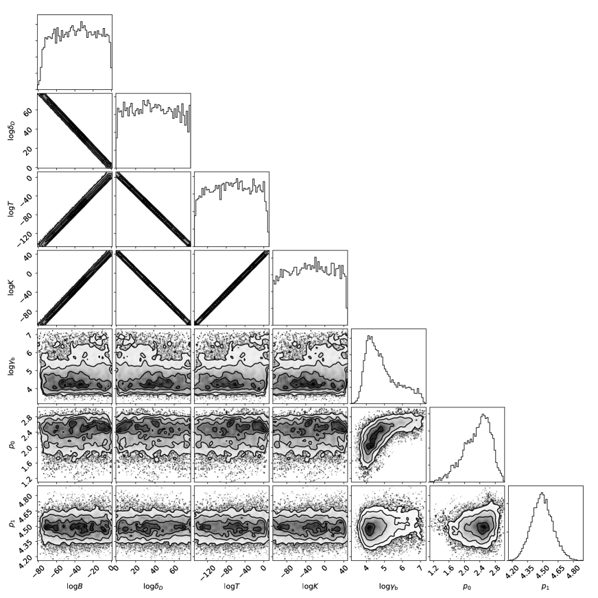
Figure 4: The one- and two-dimensional projections of the posterior probability distributions of seven parameters, $\log B$, $\log\delta_{\rm{D}}$, $\log T$, $\log K_{\rm{e}}$, $\log\gamma_{\rm{b}}$, $p_{0}$, $p_{1}$, obtained from the MCMC sample shown in Figure 15.

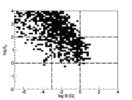
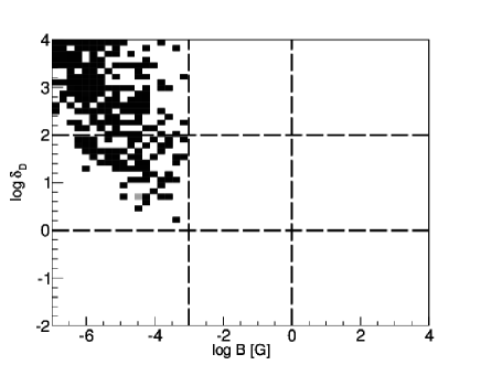
Figure 5: Posterior probability distributions on the $B$–$\delta_{\rm{D}}$ plane for the data on MJD 55598 (upper) and MJD 55623 (lower). The region bounded by the dashed lines indicate the reasonable ranges for blazars: $\log B=-3$–$0$ and $\log\delta_{\rm{D}}=0$–$2$.

4 Time-series analysis

As described in Section 3, we found strong correlations between $\log B$, $\log\delta_{\rm{D}}$, $\log T$, and $\log K_{\rm{e}}$. We need a prior distribution of only one of these parameters to uniquely determine the optimal solution. We can assume a reasonable prior distribution of $T$ from the light curve analysis. In this section, we estimate the variation time-scale by modeling the X-ray light curve of Mrk 421 with the Ornstein–Uhlenbeck (OU) process. The OU process has been used to characterize the variations observed in AGN, and also in blazars. It has been proposed that the variability of AGNs has two characteristic time-scales (Arévalo et al. (2006); McHardy et al. (2007); Kelly et al. (2011)). Sobolewska et al. (2014) reported that the $\gamma$-ray variability of blazars can also be reproduced by a model with two time-scales, a short time-scale of $\lesssim 1\;{\mathrm{d}}$ and a long time-scale of $\gtrsim 100\;{\mathrm{d}}$. In this study, we use two kinds of X-ray light curves of Mrk 421. The first was obtained from high-cadence observations by ASCA for estimating the short time-scale. The second was obtained from low-cadence observations by $\it{Swift}$-XRT for the long time-scale.

4.1 Data

We analyzed the data of Mrk 421 observed with ASCA (Tanaka et al., 1994) between MJD 50923 and 50934. We used the standard cleaned data. This satellite carries the Solid State Imaging Spectrometer (SIS; Burke et al. (1994); Yamashita et al. (1997)) and the Gas Imaging Spectrometer (GIS; Ohashi et al. (1996); Makishima et al. (1996)). We used only the SIS0 detector operating in the 1-CCD mode. We binned the light curve of Mrk 421 in intervals of 480 s, and showed it in the upper panel of Figure 6.

We created the light curve of Mrk 421 observed with $\it{Swift}$-XRT from November 2009 to April 2014 by the method described in Section 2. The light curve is shown in the lower panel of Figure 6.

4.2 OU process

We estimated the variation time-scale of the light curves by using the OU process regression. The model has three parameters: the variation time-scale, $\tau$, the variation amplitude, $A_{\rm exp}$, and the Gaussian noise variance, $\sigma^{2}$. We consider $N$ time-series data as a sample from a $N$-dimensional normal distribution, $\mathcal{N}(\bm{0},S)$, where $S$ is an $N\times N$ variance–covariance matrix. The OU process is defined with $S$ as follows:

$$S_{ij}=A_{\rm{exp}}\exp(-\frac{|t_{i}-t_{j}|}{\tau})$$ (7)

where $t_{i}-t_{j}=\Delta t$ is the time interval between the $i^{\rm th}$ and $j^{\rm th}$ epochs (Uhlenbeck, Ornstein, 1930). We consider the observed time-series data, $m(t)$, and a sample from the OU process, $f(t)$. The data is obtained as $m(t)=f(t)+\varepsilon$, where $\varepsilon$ is the error term following the normal distribution, $\mathcal{N}(0,\sigma^{2})$.

The OU process can be considered a special case of the Gaussian process (GP) with an exponential kernel. In this paper, we used the python framework, GPy, to estimate the posterior probability distributions of three parameters, $\tau$, $A_{\rm{exp}}$, and $\sigma^{2}$. We assumed a constant $\sigma^{2}$ for all light curve data which has different measurement error values. Mrk 421 is so bright in X-rays that the error of the X-ray flux is small even in the faint state. The typical fractional error is 0.02–0.04 in the X-ray faint state and less than 0.02 in the X-ray bright state, while the fractional variation amplitude is $\sim 10$. We neglected the small difference in the errors for the OU process regression. The posterior distributions were estimated with a hybrid Monte Carlo method implemented in GPy.

4.3 Estimations of variation time-scales

We optimized the three parameters of the OU process for each light curve, that is, the ASCA and $\it{Swift}$-XRT data. The light curves and best-fit models are shown in Figure 6. Figure 7 shows the posterior distributions of $\tau$. The optimal parameters of the OU process are listed in Table 2. The means and standard deviations of the MCMC samples of $\log\tau$ are $\mu=4.5$ and $\sigma=0.2$ for the ASCA data and $\mu=6.1$ and $\sigma=0.1$ for the $\it{Swift}$-XRT data.

We used them for the prior distributions of $T$ in our SED analysis, assuming that $\tau$ corresponds to the light crossing time of the emitting region. We note that the true $T$ could be shorter than $\tau$ if the observed variations are governed by time-scales longer than the light crossing time. It is unclear whether the short-term variations are present in all states or only in a specific state of Mrk 421. In this paper, we use the short time-scale estimated from the ASCA data as the shortest $T$. Since the optimal solution of the SED model depends on the assumed parameters, it is important to see the result with both the minimum and maximum $T$.

Table 2: Optimal parameters of OU process.

	ASCA	$\it{Swift}$/XRT
$\log\tau$ [s]	$4.4^{+0.3}_{-0.2}$	$6.1^{+0.1}_{-0.1}$
$A_{\rm{exp}}$	$2.9^{+0.4}_{-0.3}\times 10^{-3}$	$1.4^{+2}_{-2}\times 10^{-1}$
$\sigma^{2}$	$4^{+3}_{-2}\times 10^{-5}$	$8^{+3}_{-3}\times 10^{-3}$

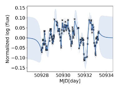
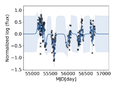
Figure 6: Data (crosses) and best-fit models (blue lines) of the OU process. The upper and lower panels show the ASCA and $\it{Swift}$-XRT data, respectively. The shaded region indicates the 95% confidence interval at each epoch.

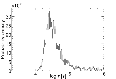
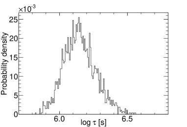
Figure 7: Posterior probability distribution of the time scale $\tau$ plotted on a logarithmic scale. The distribution was obtained from the MCMC samples shown in Figure 16.

5 Results of the SED analysis

5.1 Results obtained with the prior distribution of $T$

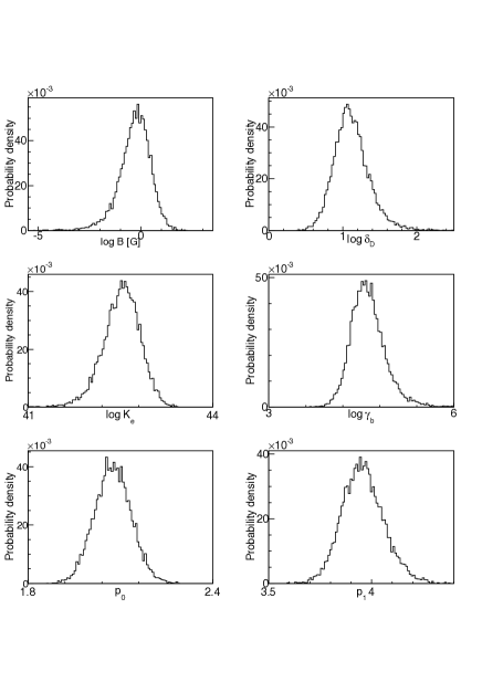
Figure 8: Probability distributions of six parameters, $\log B$, $\log\delta_{\rm{D}}$, $\log K_{\rm{e}}$, $\log\gamma_{\rm{b}}$, $p_{0}$, and $p_{1}$.

We estimated the model parameters of the SED of 31 epochs from 2009 to 2014, using the prior distribution of $T$ estimated in Section 4.

First, we show the results obtained with the prior for the short time-scale estimated from the ASCA data. The prior of $\log T$ was set to be a normal distribution with a mean of $\log T=4.5$ and a standard deviation of 0.2. Figure 8 shows their posterior distributions obtained with the data on MJD 55272, as an example. We can uniquely obtain the optimal solution and their uncertainties. The distributions are almost symmetric. In this paper, the optimal parameters are the means of each set of the MCMC samples, and the uncertainty of the optimal parameters is the 68.3$\%$ confidence interval of them.

Figure 9 shows the correlation of the X-ray flux and the parameter values obtained with the short $T$ prior. As can be seen in this figure, $\delta_{\rm D}$ is extraordinary large ($>100$) in the X-ray bright state. $\delta_{\rm D}$ becomes further large if the observed variation time-scale is longer than the light crossing time, because $\delta_{\rm D}$ is anti-correlated with $T$, as shown in Figure 4. In the X-ray faint states, the mean of $\delta_{\rm{D}}$ is 24.0 ($\log\delta_{\rm D}=1.38$), and this value is typical of the Doppler factor of Mrk 421 (e.g., Abdo et al. (2011); Bartoli et al. (2016)).

Second, we show the results obtained with the long $T$ prior. The prior of $\log T$ was a normal distribution with a mean of $\log T=6.1$ and a standard deviation of $0.1$. Figure 10 shows the results in the same way as Figure 9, but for the model with the long $T$ prior. We found that most of the bright state has acceptable $\delta_{\rm D}$ ($<100$), while the faint state tends to have atypically small $\delta_{\rm D}$ ($<10$) for SED studies of the object.

The results imply that the time-scale or the size of the dominant emitting region changed data-by-data. In other words, a model with a common prior distribution of $T$ is possibly unsuitable for the observed SED. Then, we need to restrict one of $B$, $\delta_{\rm D}$, and $K_{\rm e}$ in order to uniquely determine the solution for the SED analysis, as mentioned in Section 3.

Figure 9: Correlation of X-ray flux and the values of the parameters $\log B$, $\log\delta_{\rm{D}}$, $\log K_{\rm{e}}$, $\log\gamma_{\rm{b}}$, $p_{0}$, $p_{1}$, for the model with a prior distribution of $\log T=4.5\pm 0.2$. In the panel of $p_{1}$, we have removed the data in which $p_{1}$ was fixed to $20$. The errors of the X-ray flux are smaller than the symbol size.

Figure 10: As Figure 9 but for the model with a prior distribution of $\log T=6.1\pm 0.1$.

5.2 Results obtained with the prior distribution of $\delta_{\rm D}$

In this section we report on a SED analysis using a model with a fixed $\delta_{\rm D}$ instead of the $T$ prior. Bartoli et al. (2016) estimated $\delta_{\rm D}$ of Mrk 421 to be 10–41, based on an analysis of the SED data with a broad frequency coverage. This range of $\delta_{\rm D}$ is consistent with those found in previous investigations (Abdo et al. (2011); Shukla et al. (2012)). Here, we fixed $\delta_{\rm D}$ to be 20. We confirmed that the MCMC converged to a stationary distribution and that the posterior distributions of all parameters had a single peak, which enable us to determine the optimal solution and their uncertainties.

Figure 11 shows the correlation of the X-ray flux and the parameter values. The X-ray bright state shows small $B$ and $K_{\rm e}$ and large $T$ and $\gamma_{\rm b}$ compared with the faint state. In the X-ray bright state, $p_{0}$ exhibits an anti-correlation with the X-ray flux. $p_{0}$ remains relatively small in the faint state. No clear correlation can be seen between $p_{1}$ and X-ray flux. We note that in the panel for $p_{1}$, we removed the most samples of the bright state because $p_{1}$ of those samples was set to be 20, as mentioned in Section 3.1. These trends between the parameters and X-ray flux can be seen also in Figures 9 and 10. Thus, they are independent of the priors used in this analysis.

Examples of the observed and modeled SED are shown in Figure 12. The top and bottom panels show examples in the faint state and the bright state. We can confirm that the one-zone SSC model well reproduces the data for the set of SED considered in this section (see Section 3.3 about the discarded samples). The reduced $\chi^{2}$ for the SED model optimization are shown in Appendix 1.

Figure 11: As Figure 9 but for the model with the Doppler factor fixed to $\delta_{\rm D}=20$.

6 Discussion

6.1 General properties of SSC modeling of blazar SED

It is widely known that, in most cases, observations cannot constrain all SSC parameters because of the strong correlations between a part of them (e.g. Tavecchio et al. (1998)). To date, the detailed structure of the correlations has not explicitly shown for the optimization problem of the SSC model. Figure 4 successfully provides it in the form of the posterior probability distribution. We can obtain important properties of SSC modeling of the blazar SED from Figure 4 and results in section 3.3.

First, the optimization of the model should be performed on a logarithmic scale for $B$, $\delta_{\rm{D}}$, $T$, $K_{\rm{e}}$, and $\gamma_{\rm{b}}$. We found that $\log B$, $\log\delta_{\rm{D}}$, $\log T$, and $\log K_{\rm{e}}$ have a linear correlation in Figure 4, which can be readily sampled with the Metropolis algorithm. Several past studies using MCMC estimated the optimal parameters without TeV $\gamma$-ray data or an informative prior distribution (e.g., Yan et al. (2013); Ding et al. (2017)). We should note that non-optimal solutions can be obtained when the parameter space is insufficiently explored with MCMC.

Second, care should be taken when using priors for two or more parameters. As shown in Figure 4, a prior distribution of one of the four parameters gives constraints on the other three parameters. We have confirmed that the solution was uniquely determined when a Gaussian prior was set for $B$ or $K_{\rm e}$, instead of $T$ or $\delta_{\rm D}$. In past studies, the SSC model has sometimes been optimized with both fixed $\delta_{\rm D}$ and $T$ (e.g., Tramacere et al. (2009); Itoh et al. (2015)). Such multiple priors may lead to the optimal model parameters being overlooked. For example, in the bottom panel of Figure 5, the solution obtained with conventional constraints on the parameters (the region surrounded by the dashed lines in the figure) is different from the original optimal solution without any constraints. In such a case, we should reconsider the validity of the constraints or the model itself. Therefore, it is important to first carefully examine the posterior probability distribution in the parameter space without informative priors.

If one of $B$, $\delta_{\rm{D}}$, $T$, and $K_{\rm{e}}$ is constrained by a prior distribution or fixed value, the other parameters are determined. In other words, the values of the other parameters depend on the constraint. Care should be taken in discussions based on the values estimated by a given constraint. However, we confirmed the common trend in the parameters regardless of the fixed value or prior distribution. For example, the results in Figures 9 and 10 differ in the values of $B$, $\delta_{\rm{D}}$, and $K_{\rm{e}}$ because the centers of the prior distributions of $T$ are different, though the features of the relative variations of the parameters is common between them. Therefore, we can discuss the characteristic trend of the parameters regardless of the constraint.

Constraints are employed for $T$ and $\delta_{\rm D}$ in the study of SSC modeling of blazar SED because they can be estimated from other observations, for example, the temporal variability of the flux or that of VLBI images. As mentioned in Section 5.1, $T$ or the size of the emitting region of the bright state is distinct from that of the faint state. In Section 5.2 we reported on the results with the prior distribution of $\delta_{\rm D}$. We assumed a constant $\delta_{\rm D}$ for all epochs. However, there is a possibility that $\delta_{\rm D}$ also changed with time. In this paper, we only discuss the features of the parameter variations which are common for both the results of Section 5.1 and 5.2.

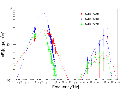
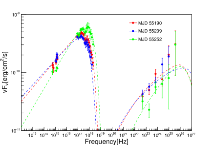
Figure 12: Examples of observed and model SEDs of Mrk 421. The model SED are indicated by the dashed lines. The left and right panels show examples in the faint and bright state, respectively. The epoch of the data is indicated in each panel.

6.2 Physical conditions of the jet

As described in Section 5.2, $\gamma_{\rm{b}}$ tends to be large in the X-ray bright state compared with the faint state. $\gamma_{\rm{b}}$ is possibly interpreted as a cooling break (Kino et al. (2002)). However, it is unlikely for our result because $p_{1}$ is estimated to be larger than that expected from this scenario ($p_{1}-p_{0}=1$), as reported in Bartoli et al. (2016): $p_{1}>5$ in most samples of the X-ray bright state and $p_{1}-p_{0}>1.5$ even in the X-ray faint state. In this case, we can consider that $\gamma_{\rm{b}}$ is effectively the maximum energy that is achieved in the acceleration process. Hence, the result indicates that the maximum energy of electrons increased in the X-ray bright state. A scenario with high-energy injection by internal shocks in relativistic shells (the shock-in-jet model) is one way to explain such variability (e.g., Spada et al. (2001)). As well as the shock-in-jet scenario, the variation in $\delta_{\rm D}$ has also been proposed as a possible origin of the observed flux variations. Figure 9 and 10 possibly support that $\delta_{\rm D}$ actually increased in the X-ray bright state. However, we emphasize that the increase in $\gamma_{\rm b}$ is seen also in Figures 9 and 10. Hence, this feature of $\gamma_{\rm b}$ is independent of the model and prior.

Itoh et al. (2015) and Bartoli et al. (2016) also reported that $\gamma_{\rm{b}}$ increased during bright X-ray flares of Mrk 421, which is consistent with our result. On the other hand, Itoh et al. (2015) described that small flares in the X-ray faint state were due to the increase in $K_{\rm e}$. However, as can be seen from Figures 9, 10, and 11, there is no positive correlation between $K_{\rm e}$ and the X-ray flux in the X-ray faint state.

In the bright state, the X-ray flux shows no clear correlation with the SED model parameters, except for $p_{0}$. It decreases with increasing X-ray flux, as can be seen all in Figures 9, 10, and 11. This is because $p_{0}$ determines the ratio between X-ray and optical fluxes, and the optical variations are fractionally much smaller than the X-ray one.

The upper panel of Figure 13 shows the total number of electrons and the X-ray flux. The total number of electrons was obtained with integrating $N_{\rm e}(\gamma)$ over $\gamma$ between $\gamma_{\rm min}$ and $\gamma_{\rm max}$ based on the results obtained with the $\delta_{\rm D}$-fixed model. The bright state has a larger number of electrons compared with the faint state. We also calculated the ratio of the electron energy density $u_{e}$ to the magnetic energy density $u_{B}$, and show it against the X-ray flux in the lower panel of Figure 13. The electron energy is larger than the magnetic energy in all samples ($u_{e}/u_{B}\gtrsim 1$), except for the data on MJD 55319 ($u_{e}/u_{B}=0.13$). The energy ratio depends on $\gamma_{\rm min}$, which we assumed $\gamma_{\rm min}=10^{2}$ in our analysis. The values of the ratio become smaller by a factor of 0.1–0.8 with a larger $\gamma_{\rm min}$ of $10^{3}$, while the ratio is greater than unity even in this case. The result of $u_{e}/u_{B}\gtrsim 1$ is consistent with previous studies of this object (Abdo et al. (2011); Bartoli et al. (2016)). The ratio is larger in the bright state than that in the faint state. This trend of $u_{e}/u_{B}$ is independent of $\gamma_{\rm min}$.

Figure 13: The total number of electrons (upper panel) and $u_{e}/u_{B}$ (lower panel) calculated from the results obtained in the $\delta_{\rm D}$-fixed model. The horizontal axis shows the X-ray flux.

The SED analysis with $\delta_{\rm D}=20$ (Section 5.2) gives $\log T=4.7$ on average of the faint state. In contrast, the bright state has a longer one: $\log T=6.3$ on average. These values are close to $\tau$ obtained from the time-series analysis with the OU process (Section 4), that is, $\log\tau=4.4_{-0.2}^{+0.3}$ from the high-cadence data and $\log\tau=6.1_{-0.1}^{+0.1}$ from the low-cadence data, as shown in Table 2. This agreement supports the idea that the variation time-scales are actually close to the light crossing time of the emitting region, and that there are two emitting regions having different sizes. The larger emitting region with the longer variation time-scale significantly contributes to the X-ray flux in the bright state.

As mentioned in section 3.1, the size of the emitting region $R$ is given with $R=c\delta_{\rm{D}}T/(1+z)$. In this study, we fixed $\delta_{\rm{D}}$ = 20. However, it is possible that $\delta_{\rm D}$ changed with time, which may make $R$ constant even if $T$ changes with time. However, this is unlikely in the present study because $\delta_{\rm D}$ would have to have changed by roughly two orders of magnitudes to cancel out the variation in $T$ between $\log T\sim 3$ and $7$. In the faint state, $R$ is calculated to be $2.9\times 10^{16}\rm{cm}$ with $\log T=4.7$. In the bright state, $R$ is calculated to be $1.1\times 10^{18}\rm{cm}$ with $\log T=6.3$. Past studies have reported that the optical emitting region typically has $R=10^{15-16}\rm{cm}$ (e.g., Tramacere et al. (2009), Abdo et al. (2011)). Therefore, the $R$ for the faint state is reasonable for the current understanding of blazars, while the $R$ for the bright state is quite large.

Spada et al. (2001) propose a model of the internal shocks between plasma shells in the AGN jets. According to this model, the first collision of the shells occurs in the upstream region of the jet at $\sim 10^{16}\,{\rm cm}$ from the central black hole. The shells then experience second and subsequent collisions in the downstream region at $\sim 10^{17-20}\,{\rm cm}$. We propose that the radiation from such a downstream region is responsible for the large emitting region of the bright state. The emergence of an additional emitting region in the 2010 outburst is also supported by the behavior of the optical polarization reported in Itoh et al. (2015). The total number of electrons in the bright state is larger than that of the faint state. This is probably due to a large emitting area of the bright state. The high $u_{e}/u_{B}$ of the bright state possibly suggests that the magnetic energy is mostly transferred into the electrons in the downstream region.

On the other hand, $p_{0}$ obtained by our analysis is larger than what is expected by the first-order Fermi acceleration in shocks ($p_{0}=2.0$–$2.2$) in the X-ray bright state. This discrepancy may suggest a scenario where the observed emission is not SSC from a single source (one-zone), but a combination of multiple SSC components (e.g., Błażejowski et al. (2005)). The two distinct variation time-scales possibly support this scenario. As mentioned in section 3.3, we discarded 10 SED samples because the optimal $B$ and $T$ are beyond the reasonable ranges. This fact also implies that multiple SSC sources are required for a significant part of the epochs.

We found notable correlations between the estimated parameters of the SSC model. Figure 14 shows the correlation between $B$, $\gamma_{\rm b}$, and $T$ obtained from the $\delta_{\rm D}$-fixed model in section 5.2. We confirmed that no other combinations of parameters exhibit such clear correlations. The negative correlation between $T$ and $B$ is reminiscent of the relation between the synchrotron cooling time-scale and magnetic field. The synchrotron cooling time-scale $t_{c}$ of an electron in a homogeneous magnetic field in the observer’s frame, can be estimated as follows:

$$t_{c}=(\delta_{\rm D})^{-1}5\times 10^{11}(1+z)^{1/2}B^{-3/2}[\rm{G}](\nu_{\rm obs}[\rm{Hz}]/\delta_{\rm D})^{-1/2}[s]$$ (8)

where $\nu_{\rm obs}$ is the observation frequency (Tucker, 1975). The cooling time-scale decreases with a larger $B$ at a given $\nu_{\rm obs}$. The shortening of the cooling time-scale in the X-ray regime may result in a decrease in the number of electrons emitting X-rays, and thereby may be responsible for the decrease in $\gamma_{\rm b}$. Hence, the correlation seen in the lower panel of Figure 14 can be explained by this scenario. However, equation (8) predicts the slope of the $\log T$–$\log B$ relation to be $-3/2$, while it is $\sim-1.0$ in the top panel of Figure 14.

Figure 14: Correlation between the three parameters $B$, $T$, and $\gamma_{\rm{b}}$. The upper panel shows the scatter plot of $B$ and $T$. The lower panel shows that of $B$ and $\gamma_{\rm{b}}$.

7 Summary

In this paper, we estimated the SSC model parameters for the SED of the blazar Mrk 421 using the Markov chain Monte Carlo (MCMC) method. We used the optical–UV (UVOT/$\it{Swift}$ and Kanata), X-ray (XRT/$\it{Swift}$), and $\gamma$-ray ($\it{Fermi}$-LAT) data sets obtained between 2009 and 2014. We found a strong correlation between the four SSC model parameters, that is, $\log B$, $\log\delta_{\rm D}$, $\log T$, and $\log K_{\rm e}$ for a model with non-informative priors. The correlation makes the model degenerate. As a result, the optimal solution can be determined uniquely only when one of the four parameters is restricted. We used two models, a model with a prior on $T$ and one with a prior on $\delta_{\rm D}$. Using a narrow prior distribution for $T$ results in unphysically large or small values for $\delta_{\rm D}$ depending on the X-ray flux. The results suggest that $T$ was large in the X-ray bright state compared with the faint state. Our SED analysis gives $\log T=6.3$ in the X-ray bright state and $\log T=4.7$ in the faint state, which are consistent to the characteristic time-scales obtained from the X-ray light curves. Those short and long $T$ correspond to the sizes of the emitting region of $2.9\times 10^{16}\rm{cm}$ and $1.1\times 10^{18}\rm{cm}$, respectively. The X-ray flares are due to an increase in $\gamma_{\rm b}$. The large emitting region in the bright state is possibly originated from the downstream area in the jet where the magnetic energy is mostly converted to electrons. On the other hand, the presence of the two kinds of emitting areas implies that the one-zone model is unsuitable to reproduce, at least a part of the observed SEDs.

The MCMC code used in this paper is available on request.

The authors thank the Suzaku, Swift, and Fermi teams for the operation, calibration, and data processing. Y.  F. was supported by JSPS KAKENHI Grant Numbers 2400000401 and 2424401400. M.  U. was supported by JSPS KAKENHI Grant Number 25120007. We would like to thank Ioannis Liodakis and Shiro Ikeda for their Valuable comments on this research. We also thank to the anonymous referee for helpful comments.

The Fermi LAT Collaboration acknowledges generous ongoing support from a number of agencies and institutes that have supported both the development and the operation of the LAT as well as scientific data analysis. These include the National Aeronautics and Space Administration and the Department of Energy in the United States, the Commissariat à l’Energie Atomique and the Centre National de la Recherche Scientifique/Institut National de Physique Nucléaire et de Physique des Particules in France, the Agenzia Spaziale Italiana and the Istituto Nazionale di Fisica Nucleare in Italy, the Ministry of Education, Culture, Sports, Science and Technology (MEXT), High Energy Accelerator Research Organization (KEK) and Japan Aerospace Exploration Agency (JAXA) in Japan, and the K. A. Wallenberg Foundation, the Swedish Research Council and the Swedish National Space Board in Sweden.

Additional support for science analysis during the operations phase is gratefully acknowledged from the Istituto Nazionale di Astrofisica in Italy and the Centre National d’Études Spatiales in France. This work was performed in part under DOE Contract DE- AC02-76SF00515.

Appendix A XRT data

Table 3 lists the epochs of the XRT data used in this paper.

Table 3: XRT data of 41 epochs

obs ID	Date (MJD)	Flux ($10^{-9}\rm{erg/cm^{2}/s}$)	Reduced ${\chi^{2}_{\rm SED}}^{\dagger}$
00030352158	55156	$1.2367^{+0.0110}_{-0.0109}$	$2.01$
00030352161	55176	$0.7883^{+0.0133}_{-0.0130}$	$2.19$
00030352164	55182	$2.4442^{+0.0239}_{-0.0237}$	$2.07$
00030352165	55186	$0.8481^{+0.0132}_{-0.0130}$	$1.25$
00030352167	55190	$1.2015^{+0.0148}_{-0.0146}$	$1.21$
00030352173	55202	$1.5379^{+0.0178}_{-0.0177}$	$1.98$
00030352175	55205	$1.1948^{+0.0105}_{-0.0104}$	$3.41$
00030352176	55207	$0.9499^{+0.0010}_{-0.0099}$	$1.24$
00030352177	55209	$1.0231^{+0.0132}_{-0.0131}$	$1.88$
00030352178	55210	$1.8317^{+0.0168}_{-0.0166}$	$1.58$
00030352179	55211	$2.1356^{+0.0208}_{-0.0208}$	$3.15$
00030352182	55212	$0.4834^{+0.0106}_{-0.0109}$	$1.61$
00030352183	55213	$0.6088^{+0.0074}_{-0.0074}$	$1.87$
00030352185	55215	$1.6785^{+0.0203}_{-0.0202}$	$1.36$
00030352188	55220	$0.5938^{+0.0124}_{-0.0123}$	$1.32$
00030352195	55230	$0.4209^{+0.0095}_{-0.0924}$	$1.25$
00030352198	55235	$0.7029^{+0.0119}_{-0.0118}$	$1.43$
00030352201	55238	$0.8301^{+0.0123}_{-0.0122}$	$2.01$
00030352203	55239	$1.7743^{+0.0176}_{-0.0176}$	$1.58$
00030352213	55252	$1.7707^{+0.0199}_{-0.0198}$	$0.94$
00030352217	55257	$2.2342^{+0.0213}_{-0.0212}$	$1.73$
00030352221	55261	$1.0977^{+0.0134}_{-0.0134}$	$1.49$
00030352230	55272	$0.4402^{+0.0329}_{-0.0300}$	$0.98$
00030352233	55275	$0.7999^{+0.0108}_{-0.0107}$	$1.54$
00030352242	55287	$0.7622^{+0.0134}_{-0.0133}$	$1.24$
00031202007	55290	$1.1001^{+0.0187}_{-0.0186}$	$1.38$
00031202015	55309	$0.8228^{+0.0149}_{-0.0140}$	$1.12$
00031202016	55312	$1.1803^{+0.0165}_{-0.0164}$	$1.24$
00031202019	55318	$1.1946^{+0.0137}_{-0.0137}$	$1.42$
00031202020	55319	$0.9743^{+0.0127}_{-0.0126}$	$1.45$
00031202032	55339	$1.3999^{+0.0155}_{-0.0154}$	$1.44$
00031202060	55568	$0.2592^{+0.0120}_{-0.0110}$	$1.57$
00031202061	55570	$0.2403^{+0.0078}_{-0.0074}$	$1.25$
00031202076	55598	$0.1414^{+0.0080}_{-0.0071}$	$0.84$
00031202087	55623	$0.1741^{+0.0063}_{-0.0060}$	$3.74$
00031202094	55633	$0.2189^{+0.0083}_{-0.0078}$	$3.33$
00035014025	56300	$0.1525^{+0.0086}_{-0.0076}$	$0.99$
00035014032	56304	$0.3149^{+0.0099}_{-0.0094}$	$1.34$
00035014072	56414	$0.4501^{+0.0055}_{-0.0054}$	$1.19$
00035014076	56428	$0.2499^{+0.0082}_{-0.0078}$	$1.14$
00035014108	56708	$0.4167^{+0.0159}_{-0.0102}$	$1.35$
†Reduced $\chi^{2}$ of the SED analysis shown in section 5.2

Appendix B Trace plots

Figures 15 and 16 show the trace plots of the MCMC samples for the SED analysis of the data on MJD 55598 with non-informative prior (section 3.3) and for the OU process regression of the X-ray light curve (section 4.3).

We tested the convergence of the MCMC samples by using the Gelman and Rubin’s convergence diagnostic (Gelman & Rubin (1992); Brooks & Gelman (1997)). The method gives the potential scale reduction factor (PSRF) calculated from the means and variances of multiple Markov chains with different initial values. We can be confident that convergence has been achieved if PSRF $<1.1$ for all parameters. For example, using the MCMC samples shown in Figure 15, we calculated PSRF to be 1.015, 1.016, 1.017, 1.016, 1.018, 1.049, and 1.018 for the parameter, $\log B$, $\log\delta_{\rm D}$, $\log T$, $\log K_{\rm e}$, $\log\gamma_{\rm b}$, $p_{0}$, and $p_{1}$, respectively, from five chains each of which has $8\times 10^{4}$ samples. We confirmed that the PSRF criterion was satisfied in all cases in this paper.

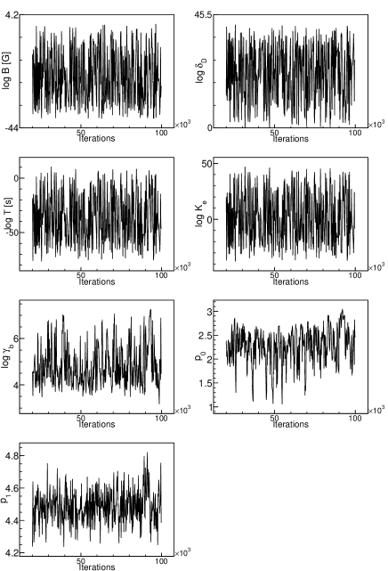
Figure 15: Trace plots of seven parameters, $\log B$, $\log\delta_{\rm{D}}$, $\log T$, $\log K_{\rm{e}}$, $\log\gamma_{\rm{b}}$, $p_{0}$, $p_{1}$, obtained with MCMC and a model with non-informative priors. The data on MJD 55598 was used. The horizontal and vertical axes indicate the iteration of the MCMC algorithm and each parameter value. The algorithm was iterated $10^{5}$ times. We discarded the first $2.0\times 10^{4}$ steps as burn-in.

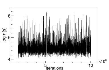
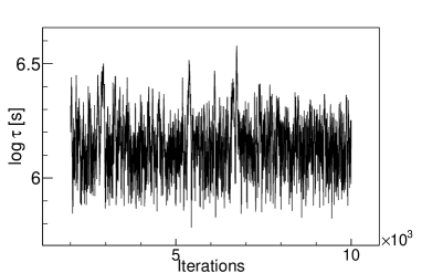
Figure 16: Trace plots of the time scale $\tau$ obtained with MCMC. The left and right panels show the results for the ASCA and $\it{Swift}$-XRT data, respectively.

References

- Abdo et al. (2011) Abdo, A. A., Ackermann, M., Ajello, M., Baldini, L., Ballet, J., Barbiellini, G., Bastieri, D., Bechtol, K., et al. 2011, ApJ, 736, 131
- Acero et al. (2015) Acero, F., Ackermann, M., Ajello, M., Albert, A., Atwood, W., Axelsson, M., Baldini, L., Ballet, J., et al. 2015, The Astrophysical Journal Supplement Series, 218, 23
- Acero et al. (2016) Acero, F., Ackermann, M., Ajello, M., Albert, A., Baldini, L., Ballet, J., Barbiellini, G., Bastieri, D., et al. 2016, ApJS, 223, 26
- Aielli et al. (2010) Aielli, G., Bacci, C., Bartoli, B., Bernardini, P., Bi, X. J., Bleve, C., Branchini, P., Budano, A., et al. 2010, ApJ, 714, L208
- Arévalo et al. (2006) Arévalo, P., Papadakis, I. E., Uttley, P., McHardy, I. M., & Brinkmann, W. 2006, MNRAS, 372, 401
- Atwood et al. (2009) Atwood, W. B., Abdo, A. A., Ackermann, M., Althouse, W., Anderson, B., Axelsson, M., Baldini, L., Ballet, J., et al. 2009, ApJ, 697, 1071
- Atwood et al. (2013) Atwood, W. B., Baldini, L., Bregeon, J., Bruel, P., Chekhtman, A., Cohen-Tanugi, J., Drlica-Wagner, A., Granot, J., et al. 2013, ApJ, 774, 76
- Bartoli et al. (2011) Bartoli, B., Bernardini, P., Bi, X., Bleve, C., Bolognino, I., Branchini, P., Budano, A., Melcarne, A. C., et al. 2011, The Astrophysical Journal, 734, 110
- Bartoli et al. (2016) Bartoli, B., Bernardini, P., Bi, X. J., Cao, Z., Catalanotti, S., Chen, S. Z., Chen, T. L., Cui, S. W., et al. 2016, ApJS, 222, 6
- Błażejowski et al. (2005) Błażejowski, M., Blaylock, G., Bond, I., Bradbury, S., Buckley, J., Carter-Lewis, D., Celik, O., Cogan, P., et al. 2005, The Astrophysical Journal, 630, 130
- Böttcher (2007) Böttcher, M. 2007, Ap&SS, 309, 95
- Böttcher et al. (2013) Böttcher, M., Reimer, A., Sweeney, K., & Prakash, A. 2013, The Astrophysical Journal, 768, 54
- Brooks & Gelman (1997) Brooks, S. P., Gelman, A. 1997. Journal of Computational and Graphical Statistics, 7, 434
- Burke et al. (1994) Burke, B., Mountain, R., Daniels, P., Cooper, M., & Dolat, V. 1994, IEEE transactions on nuclear science, 41, 375
- Burrows et al. (2005) Burrows, D. N., Hill, J. E., Nousek, J. A., Kennea, J. A., Wells, A., Osborne, J. P., Abbey, A. F., Beardmore, A., et al. 2005, Space Sci. Rev., 120, 165
- Cardelli et al. (1989) Cardelli, J. A., Clayton, G. C., & Mathis, J. S. 1989, The Astrophysical Journal, 345, 245
- Ding et al. (2017) Ding, N., Zhang, X., Xiong, D. R., & Zhang, H. J. 2017, MNRAS, 464, 599
- Donnarumma et al. (2009) Donnarumma, I., Vittorini, V., Vercellone, S., del Monte, E., Feroci, M., D’Ammando, F., Pacciani, L., Chen, A. W., et al. 2009, ApJ, 691, L13
- Finke et al. (2008) Finke, J. D., Dermer, C. D., & Böttcher, M. 2008, The Astrophysical Journal, 686, 181
- Fossati et al. (2008) Fossati, G., Buckley, J., Bond, I., Bradbury, S., Carter-Lewis, D., Chow, Y., Cui, W., Falcone, A., et al. 2008, The Astrophysical Journal, 677, 906
- Fossati et al. (1998) Fossati, G., Maraschi, L., Celotti, A., Comastri, A., & Ghisellini, G. 1998, MNRAS, 299, 433
- Gehrels et al. (2004) Gehrels, N., Chincarini, G., Giommi, P., Mason, K. O., Nousek, J. A., Wells, A. A., White, N. E., Barthelmy, S. D., et al. 2004, ApJ, 611, 1005
- Gelman & Rubin (1992) Gelman, A., Rubin, D B. 1992, Statistical Science, 7, 457
- Ghisellini et al. (2009) Ghisellini, G., Tavecchio, F., & Ghirlanda, G. 2009, MNRAS, 399, 2041
- Haario et al. (2001) Haario, H., Saksman, E., & Tamminen, J. 2001, Bernoulli, 7, 223
- Itoh et al. (2015) Itoh, R., Fukazawa, Y., Tanaka, Y. T., Kawabata, K. S., Takaki, K., Hayashi, K., Uemura, M., Ui, T., et al. 2015, PASJ, 67, 45
- Kawabata et al. (2008) Kawabata, K. S., Nagae, O., Chiyonobu, S., Tanaka, H., Nakaya, H., Suzuki, M., Kamata, Y., Miyazaki, S., et al. 2008, in Ground-based and Airborne Instrumentation for Astronomy II Vol. 7014 of Proc. SPIE 70144L
- Kelly et al. (2009) Kelly, B. C., Bechtold, J., & Siemiginowska, A. 2009, The Astrophysical Journal, 698, 895
- Kelly et al. (2011) Kelly, B. C., Sobolewska, M., & Siemiginowska, A. 2011, The Astrophysical Journal, 730, 52
- Kino et al. (2002) Kino, M., Takahara, F., & Kusunose, M. 2002, The Astrophysical Journal, 564, 97
- Lockman, Savage (1995) Lockman, F. J. & Savage, B. D. 1995, ApJS, 97, 1
- Makishima et al. (1996) Makishima, K., Tashiro, M., Ebisawa, K., Ezawa, H., Fukazawa, Y., Gunji, S., Hirayama, M., Idesawa, E., et al. 1996, Publications of the Astronomical Society of Japan, 48, 171
- McHardy et al. (2007) McHardy, I. M., Arévalo, P., Uttley, P., Papadakis, I. E., Summons, D. P., Brinkmann, W., & Page, M. J. 2007, MNRAS, 382, 985
- Ohashi et al. (1996) Ohashi, T., Ebisawa, K., Fukazawa, Y., Hiyoshi, K., Horii, M., Ikebe, Y., Ikeda, H., Inoue, H., et al. 1996, Publications of the Astronomical Society of Japan, 48, 157
- Paggi et al. (2009) Paggi, A., Cavaliere, A., Vittorini, V., & Tavani, M. 2009, A&A, 508, L31
- Poole et al. (2008) Poole, T. S., Breeveld, A. A., Page, M. J., Landsman, W., Holland, S. T., Roming, P., Kuin, N. P. M., Brown, P. J., et al. 2008, MNRAS, 383, 627
- Punch et al. (1992) Punch, M., Akerlof, C. W., Cawley, M. F., Chantell, M., Fegan, D. J., Fennell, S., Gaidos, J. A., Hagan, J., et al. 1992, Nature, 358, 477
- Robbins & Monro (1951) Robbins, H. & Monro, S. 1951, Statistics, 22, 400
- Roberts et al. (1997) Roberts, G. O., Gelman, A., Gilks, W. R. 1997, Annals of Applied Probability, 7, 110
- Roming et al. (2005) Roming, P. W. A., Kennedy, T. E., Mason, K. O., Nousek, J. A., Ahr, L., Bingham, R. E., Broos, P. S., Carter, M. J., et al. 2005, Space Sci. Rev., 120, 95
- Schlafly & Finkbeiner (2011) Schlafly, E. F. & Finkbeiner, D. P. 2011, ApJ, 737, 103
- Shukla et al. (2012) Shukla, A., Chitnis, V. R., Vishwanath, P. R., Acharya, B. S., Anupama, G. C., Bhattacharjee, P., Britto, R. J., Prabhu, T. P., Saha, L., & Singh, B. B. 2012, A&A, 541, A140
- Sobolewska et al. (2014) Sobolewska, M. A., Siemiginowska, A., Kelly, B. C., & Nalewajko, K. 2014, ApJ, 786, 143
- Spada et al. (2001) Spada, M., Ghisellini, G., Lazzati, D., & Celotti, A. 2001, MNRAS, 325, 1559
- Tanaka et al. (1994) Tanaka, Y., Inoue, H., & Holt, S. S. 1994, Publications of the Astronomical Society of Japan, 46, L37
- Tavecchio et al. (1998) Tavecchio, F., Maraschi, L., & Ghisellini, G. 1998, The Astrophysical Journal, 509, 608
- Tramacere et al. (2009) Tramacere, A., Giommi, P., Perri, M., Verrecchia, F., & Tosti, G. 2009, A&A, 501, 879
- Tucker (1975) Tucker, W. 1975, Radiation processes in astrophysics (Cambridge, Mass., MIT Press)
- Uhlenbeck, Ornstein (1930) Uhlenbeck, G. E. & Ornstein, L. S. 1930, Physical review, 36, 823
- Urry, Padovani (1995) Urry, C. M. & Padovani, P. 1995, PASP, 107, 803
- Vianello et al. (2015) Vianello, G., Lauer, R. J., Younk, P., Tibaldo, L., Burgess, J. M., Ayala, H., Harding, P., Hui, M., Omodei, N., & Zhou, H. 2015, Proceedings of the 34th International Cosmic Ray Conference (ICRC2015), 1042 (arXiv:1507.08343)
- Yamashita et al. (1997) Yamashita, A., Dotani, T., Bautz, M., Crew, G., Ezuka, H., Gendreau, K., Kotani, T., Mitsuda, K., et al. 1997, IEEE Transactions on Nuclear Science, 44, 847
- Yan et al. (2013) Yan, D., Zhang, L., Yuan, Q., Fan, Z., & Zeng, H. 2013, The Astrophysical Journal, 765, 122