Numerical solutions to Einstein’s equations in a shearing-dust Universe:
a code comparison

Abstract

A number of codes for general-relativistic simulations of cosmological structure formation have been developed in recent years. Here we demonstrate that a sample of these codes produce consistent results beyond the Newtonian regime. We simulate solutions to Einstein’s equations dominated by gravitomagnetism — a vector-type gravitational field that doesn’t exist in Newtonian gravity and produces frame-dragging, the leading-order post-Newtonian effect. We calculate the coordinate-invariant effect on intersecting null geodesics by performing ray tracing in each independent code. With this observable quantity, we assess and compare each code’s ability to compute relativistic effects.

I Introduction

The flat $\Lambda$ Cold Dark Matter ($\Lambda$CDM) model is the backbone of modern cosmology. Originally proposed in the context of the inflationary scenario Peebles (1984) and to accommodate for observations of structures on large scales Efstathiou et al. (1990), it has emerged as the concordance cosmological model Spergel et al. (2003); Tegmark et al. (2004) after the discovery of the accelerating expansion of the Universe Riess et al. (1998); Perlmutter et al. (1999). Theoretically, $\Lambda$CDM rests on three main pillars: i) based on general relativity (GR) with a cosmological constant $\Lambda$, a Friedmann-Lemaître-Robertson-Walker (FLRW) metric is adopted as the description of the Universe on average, on the assumption of large-scale statistical homogeneity and isotropy; ii) the relativistic perturbations of this background model are used to describe small inhomogeneities at large scales and early times, e.g. cosmic microwave background fluctuations; iii) Newtonian dynamics is used to model structure formation at late times and on small scales, where nonlinearity in the matter distribution is important.

On these bases, $\Lambda$CDM successfully explains the majority of our cosmological observations in a surprisingly simple framework Aghanim et al. (2018); Alam et al. (2017). Yet $\Lambda$CDM faces a number of challenges, theoretical and observational. While a cosmological constant representing vacuum energy Lemaître (1931, 1934) is the simplest possible form of dark energy, the measured value is difficult to justify from a theory standpoint Adler et al. (1995); Weinberg (1989); Martin (2012). With the continuous improvement of cosmological observations, a number of tensions have started to emerge (see, e.g. Buchert et al., 2016), particularly between low and high redshift measurements of some cosmological parameters. For example, a significant tension exists between supernovæ Riess et al. (2018) and cosmic microwave background measurements Aghanim et al. (2018) of the present Hubble expansion rate, $H_{0}$ Riess et al. (2019). The former depends on calibration on the cosmic distance ladder Lemos et al. (2019), and the latter depends on assuming $\Lambda$CDM as cosmological model. Also assuming $\Lambda$CDM, a tension is present between high and low redshift observations of $\sigma_{8}$, the parameter measuring the growth of structures Battye et al. (2015); Douspis et al. (2018). Recently, some evidence for a spatially curved universe has been claimed Handley (2019); Di Valentino et al. (2019) and disputed Efstathiou and Gratton (2020), with some authors suggesting the possibility of a structure formation-induced curvature Bolejko (2017). Motivated theoretically and because of these tensions, a number of alternatives to $\Lambda$CDM have been considered. These range from an interacting vacuum scenario (see, e.g. Salvatelli et al., 2014; Wang et al., 2014; Martinelli et al., 2019; Hogg et al., 2020, and references therein), to scalar fields Copeland et al. (2006) and modified gravity models (see e.g. Clifton et al., 2012; Joyce et al., 2016; Ezquiaga and Zumalacárregui, 2017; Frusciante and Perenon, 2019, and references therein). However, $\Lambda$CDM is still largely preferred when Bayesian model comparisons are carried out Heavens et al. (2017); Renk et al. (2017); Zhao et al. (2017); Lazkoz et al. (2018); Di Valentino et al. (2020).

With the increasing precision of current and upcoming cosmological surveys Euc (2020); LSS (2020); SKA (2020), the $\Lambda$CDM model will be truly tested. In view of these future observations and their target 1% precision, current state-of-the-art cosmological N-body simulations of structure formation aim at the same precision in theoretical predictions. However, considering that these N-body simulations are mostly based on the Newtonian approximation in lieu of full GR, it is timely to address the possibility that some percent-level GR effects may be missed, potentially biasing the inferred likelihood of cosmological parameters. Understanding the role of general-relativistic effects on observations will thus be crucial in correctly interpreting these precision data.

While the extensions and alternatives to $\Lambda$CDM mentioned above explore new physics, some explore the inclusion of existing physics that is neglected by the standard cosmological model. Previous efforts to investigate the role of GR effects in numerical cosmology have included simplifying symmetries (e.g. Torres et al., 2014; Rekier et al., 2015). In recent years, a number of general-relativistic codes with no assumed symmetries have been developed for cosmology, employing either a formally exact treatment of the metric Loffler et al. (2012); Giblin et al. (2016a); Bentivegna and Bruni (2016); Macpherson et al. (2017); Clesse et al. (2017); East et al. (2018); Daverio et al. (2019) or an approximate scheme Adamek et al. (2016a); Barrera-Hinojosa and Li (2020a). These tools provide new ways to study aspects of GR beyond the limited scope of known analytic solutions and perturbative expansions around them. For instance, they have been applied to quantify gravitational back-reaction of small-scale structures Bentivegna and Korzynski (2012, 2013); Macpherson et al. (2018); Adamek et al. (2019a); Giblin et al. (2019a); Macpherson et al. (2019), light-cone projection effects Giblin et al. (2016b); Bentivegna et al. (2017); Giblin et al. (2017); Adamek et al. (2019b), and the impact of relativistic species Adamek et al. (2017a, b) on the evolution and observation of large-scale structure. These codes have proven themselves reliable through comparisons to both linearized and exact GR solutions (e.g. Adamek et al. (2014, 2016b); Mertens et al. (2016); Bentivegna (2017)), and have in turn been used to validate the applicability of traditional Newtonian simulations to cosmology in a weak-field limit (e.g. Adamek et al. (2016c); East et al. (2018, 2019)).

Here, we compare several codes within a controlled setup that features an artificially large gravitomagnetic vector potential as part of the metric, generating a frame-dragging effect. Connected to rotation of masses, frame dragging has been measured in the gravitational field of the Earth Everitt et al (2011). Gravitomagnetism and frame dragging are purely relativistic and absent from Newtonian gravity, a theory based on a single scalar potential (see however Bruni et al. (2014) where this effect is computed from a Newtonian code using a post-Friedmann approximation Milillo et al. (2015)). There are only a few known analytic solutions that exhibit frame-dragging — e.g. the Kerr and Kerr-Newman solutions — although the effect is ubiquitous in GR, for example in rotating neutron stars (see, e.g. Berti et al., 2005). Numerical cosmological solutions with large frame-dragging effects have also been studied Giblin et al. (2019b).

In the limit where linear cosmological perturbation theory provides an accurate description of the behavior of a spacetime, frame-dragging is associated with the presence of vector modes Bardeen (1980); Bruni et al. (1992) and is well understood and under analytic control. However, vector modes may also be sourced through nonlinear processes (e.g. Bruni et al., 1997; Matarrese et al., 1998; Lu et al., 2009; Thomas et al., 2015; Jelic-Cizmek et al., 2018; Rampf et al., 2016; Gressel et al., 2019), potentially interfering with our ability to measure phenomena such as primordial gravitational waves of sufficiently small amplitude Saga (2016). They can also produce a gradient in the matter density field Ellis et al. (1990). While such vector modes are not expected to be a dominant contribution to either the dynamics of our Universe or the propagation of information through it, simulating such a physical system nevertheless provides us with a way to explore the regime of validity of approximate numerical and analytic models. At the nonlinear level, we must seek to validate both perturbation theory and approximate numerical approaches against fully general-relativistic calculations.

In this work, we do precisely this. We describe and perform a comparison between linear theory, simulations that use an approximate treatment of Einstein’s equations to model nonlinear effects, and numerical relativity simulations that provide numerically exact solutions to Einstein’s equations. We focus our comparison on the purely relativistic frame-dragging effect. It would of course be interesting to study other relativistic effects relevant for cosmology, e.g. in nonlinear structure formation or gravitational waves. While these lie beyond the scope of this paper, we emphasise that switching on gravitomagnetism goes a long way, because all relativistic degrees of freedom are excited once nonlinearity becomes relevant. On this basis, it seems reasonable to expect that the level of agreement among codes in this test should be a good indication of what to expect in other regimes.

We present the initial data for our simulations in Section II, describe the observables we compute in Section III, give an overview of the different computational frameworks in Section IV, discuss our results in Section V and conclude in Section VI.

Unless otherwise stated, we use Latin indices to represent spatial indices, which take values $1,2,$ and $3$, and Greek indices to represent space-time indices which take values $0,1,2$, and $3$, with repeated indices implying summation. We set the speed of light $c=1$.

II Initial data

GR admits a well-posed initial-value formulation (see, e.g. Wald, 1984). A consequence of this is that in cosmological simulations we don’t need to specify an a-priori fixed background. We choose coordinates such that our initial Cauchy surface is described by a fixed coordinate time, $t{=t_{\ast}}$. The line element in the 3+1 decomposition is Alcubierre (2008)

$$g_{\mu\nu}dx^{\mu}dx^{\nu}=-\alpha^{2}dt^{2}+\gamma_{ij}\left(dx^{i}+\beta^{i}dt\right)\left(dx^{j}+\beta^{j}dt\right)\,,$$ (1)

where $x^{i}\in\left\{x,y,z\right\}$ are coordinates on the three-dimensional space-like hypersurface, $\alpha$ is the lapse function, and $\beta^{i}$ is the shift vector. While we will set initial conditions non-perturbatively, we can draw a connection to linear perturbation theory both for intuition and a comparison. We choose the initial lapse, shift, spatial metric, and extrinsic curvature to be, respectively,

$$\alpha_{\ast} = 1\,,$$ (2)

$$\beta^{i}_{\ast} = 0\,,$$ (3)

$$\gamma^{\ast}_{ij} = \begin{pmatrix}1&\frac{b}{H_{\ast}L}\cos\frac{2\pi y}{L}&0\\ \frac{b}{H_{\ast}L}\cos\frac{2\pi y}{L}&1+\frac{b^{2}}{H_{\ast}^{2}L^{2}}\cos^{2}\frac{2\pi y}{L}&0\\ 0&0&1\end{pmatrix}\,,$$ (4)

$$K^{\ast}_{ij} = -\begin{pmatrix}H_{\ast}&\frac{b}{4L}\cos\frac{2\pi y}{L}&0\\ \frac{b}{4L}\cos\frac{2\pi y}{L}&H_{\ast}-\frac{b^{2}}{2H_{\ast}L^{2}}\cos^{2}\frac{2\pi y}{L}&0\\ 0&0&H_{\ast}\end{pmatrix}\,.~{}$$ (5)

This can be regarded as a snapshot at an initial time $t_{\ast}$ of an exact perturbation of a reference Einstein-de Sitter (EdS) model with Hubble expansion rate $H_{\ast}$. Here, $L$ is the characteristic length scale of the vector perturbation that also determines the size of the simulation volume (the initial conditions are compatible with periodic boundary conditions that identify $y=L$ with $y=0$), $b$ is a dimensionless amplitude, and the asterisk indicates that a quantity is evaluated on the initial Cauchy surface. The surface has vanishing three-dimensional Riemann tensor ($\gamma_{ij}^{\ast}$ is the Euclidean metric in unusual coordinates) but non-trivial extrinsic curvature. The connection with linear perturbation theory will become apparent shortly.

Having fixed the initial conditions for the metric we can proceed by solving the Hamiltonian and momentum constraint equations on the initial surface to obtain valid initial data for the matter. We assume that the matter can be described (at least initially) as a perfect fluid with vanishing pressure, such that the stress-energy tensor is given by

$$T^{\mu\nu}=\rho_{0}u^{\mu}u^{\nu}\,,$$ (6)

where $\rho_{0}$ is the rest mass-energy density and $u^{\mu}$ is the four-velocity of the fluid. For collisionless matter the fluid description can break down at some point in the evolution due to stream crossing, and we will comment on this issue later.

The Hamiltonian and momentum constraint equations are, respectively,

$${}^{(3)}\!R+K^{2}-K_{ij}K^{ij} = 16\pi G\alpha^{2}\rho_{0}\left(u^{0}\right)^{2}\,,$$ (7)

$$D_{j}\left(K^{ij}-\gamma^{ij}K\right) = 8\pi G\alpha\rho_{0}u^{i}u^{0}\,,$$ (8)

where the 3-curvature ${}^{(3)}\!R$ and covariant derivative $D_{j}$ are associated with the 3-metric $\gamma_{ij}$, and $K=\gamma^{ij}K_{ij}$. Together with the mass-shell condition $g_{\mu\nu}u^{\mu}u^{\nu}=-1$, this yields a closed system of equations from which we can determine $\rho_{0}^{\ast}$ and $u^{\mu}_{\ast}$. Solving this system, given the initial conditions (2), (3), (4), and (5), we obtain

$$\rho_{0}^{\ast}=3\frac{\left(16H_{\ast}^{2}L^{2}-3b^{2}\cos^{2}\frac{2\pi y}{L}\right)^{2}-64\pi^{2}b^{2}\sin^{2}\frac{2\pi y}{L}}{128\pi GL^{2}\left(16H_{\ast}^{2}L^{2}-3b^{2}\cos^{2}\frac{2\pi y}{L}\right)}\,,$$ (9)

$$u_{\ast}^{x}=-\frac{8\pi b\sin\frac{2\pi y}{L}}{\sqrt{\left(16H_{\ast}^{2}L^{2}-3b^{2}\cos^{2}\frac{2\pi y}{L}\right)^{2}-64\pi^{2}b^{2}\sin^{2}\frac{2\pi y}{L}}}\,,$$ (10)

and $u_{\ast}^{y}=u_{\ast}^{z}=0$.

It is worth noting at this point that values $b>2H_{\ast}^{2}L^{2}/\pi$ are unphysical, as they violate the weak energy condition $\rho_{0}^{\ast}>0$ at $t_{\ast}$. For $H_{\ast}L>\pi\sqrt{2/3}$, i.e. for exact perturbations outside the Hubble horizon, the physical range of $b$ is even more restricted, becoming bounded from above by $b<4\sqrt{3H_{\ast}^{2}L^{2}-\pi^{2}}/3$.

All of the explicit expressions given so far are of course valid in the coordinate system we chose, in particular with $\beta^{i}=0$. We can therefore use these expressions directly to set the initial conditions in those simulations that use such coordinates. However, in some simulations we will instead use the coordinates of the so-called Poisson gauge in which vector perturbations are completely carried by the shift. In this gauge we denote the line element as

$$\tilde{g}_{\mu\nu}d\tilde{x}^{\mu}d\tilde{x}^{\nu}=a^{2}(\tilde{t})\bigl{[}-e^{2\psi}d\tilde{t}^{2}+{\tilde{\gamma}^{ij}B_{i}B_{j}d\tilde{t}^{2}}-2B_{i}d\tilde{x}^{i}d\tilde{t}\bigr{.}\\ \bigl{.}+e^{-2\phi}\delta_{ij}d\tilde{x}^{i}d\tilde{x}^{j}+h_{ij}d\tilde{x}^{i}d\tilde{x}^{j}\bigr{]}\,,$$ (11)

where $a(\tilde{t})$ is the scale factor of the reference EdS model, the shift $B_{i}$ is the transverse gravitomagnetic vector potential, $h_{ij}$ is transverse and traceless, and $\tilde{\gamma}^{ij}=(e^{-2\phi}\delta_{ij}+h_{ij})^{-1}$ is the inverse of the spatial metric.

For the particular initial data chosen, a closed expression for the coordinate transformation $x^{\mu}\mapsto\tilde{x}^{\mu}$ is given by

$$\tilde{t} = t\,,$$ (12)

$$\tilde{x} = x+\frac{b}{2\pi}\left[\frac{1}{H_{\ast}}-\frac{3}{2}\left(t-t_{\ast}\right)\right]\sin\frac{2\pi y}{L}\,,$$ (13)

$$\tilde{y} = y\,,$$ (14)

$$\tilde{z} = z\,,$$ (15)

for an infinitesimal $(t-t_{\ast})$ around the initial Cauchy hypersurface. The metric variables in Poisson gauge are then initially given by

$$B_{i}^{\ast}=-\begin{pmatrix}\frac{3b}{4\pi}\sin\frac{2\pi y}{L}\\ 0\\ 0\end{pmatrix}\,,$$ (16)

and ${\psi_{\ast}=}~{}\phi_{\ast}=h_{ij}^{\ast}=0$. We note that from the point of view of the Poisson gauge, the extrinsic curvature is only needed to provide the initial data for the propagating gravitational waves (i.e. the free part, or homogeneous solution, of $h_{ij}$). Due to the weak-field approximation, this part completely decouples from the remaining dynamics in gevolution while it is neglected from the outset in gramses — which are the two codes detailed below that take their initial data in this coordinate system. Therefore the extrinsic curvature in Poisson gauge is not required for setting initial conditions in this work.

From (16) it is clear that the dimensionless parameter $b$ measures the strength of the gravitomagnetic field on the initial hypersurface. Neglecting $b^{2}$ terms in the above expressions we obtain initial conditions for the first-order solutions in the two gauges. We discuss this further in Section III.1 below.

III Behavior of observables

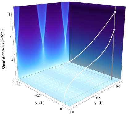
We now want to construct an observable that can be used to “measure” the frame-dragging effect even in the nonperturbative case. Consider an observer comoving with the fluid and located at a point of symmetry where spacetime is invariant under a parity transformation. Without loss of generality we can choose the observer to be located at the origin $x_{O}=y_{O}=z_{O}=0$. Now consider two events $A$ and $B$ on the initial hypersurface that emit a flash of light in all directions. Within the coordinate system that we introduced on the initial hypersurface, these events shall be located at $x_{A}=x_{O}-L,y_{A}=y_{O},z_{A}=z_{O}$ and $x_{B}=x_{O},y_{B}=y_{O}-L,z_{B}=z_{O}$. The null geodesics that connect each of these two events with the worldline of the observer get “lensed” by the frame-dragging effect (see Figure 1 for an illustration). The ray coming from $A$ travels close to a plane of symmetry, while the ray coming from $B$ travels almost orthogonal to it. They will therefore be affected in different ways. One effect is that the angle $\vartheta$ between the two incoming rays is not exactly 90 degrees in the frame of the observer. The non-vanishing dot-product

$$\cos\vartheta=\left.\frac{k^{\mu}_{A}e_{\mu}^{i}\delta_{ij}k^{\nu}_{B}e_{\nu}^{j}}{k^{\mu}_{A}u_{\mu}k^{\nu}_{B}u_{\nu}}\right|_{O}$$ (17)

of the two direction vectors (in the observer’s rest frame) is therefore an observable that directly relates to the frame-dragging effect. Here $u^{\mu}$ is the observer’s four-velocity (which coincides with that of the fluid in this case), $k^{\mu}_{A}$, $k^{\nu}_{B}$ denote the two null vectors of the incoming geodesics, and the $e^{i}_{\mu}$ are the basis vectors of the Fermi frame that, up to rotations, is fixed by the requirement that $u^{\mu}e_{\mu}^{i}=0$ and $g^{\mu\nu}e_{\mu}^{i}e_{\nu}^{j}=\delta^{ij}$.

III.1 Linear regime

We first analyze a solution in the regime where the amplitude of the perturbation $b$ is small and a linear treatment — i.e. a first-order expansion in $b$ about an EdS background — is therefore a good approximation. In this regime it is convenient to work with first-order gauge-invariant variables, an approach pioneered by Bardeen in his seminal work Bardeen (1980). If matter has vanishing pressure, the first-order gauge-invariant vector mode decays like $1/a^{2}$. Noting that $a\propto t^{2}$ if the Universe is matter dominated (where $t$ is conformal time), we find that the linear solution for a harmonic slicing and with initial conditions given by eqs. (2)–(5) is

$$\alpha=\frac{t^{2}}{t_{\ast}^{2}}\,,\quad\gamma_{ij}=\begin{pmatrix}\frac{t^{4}}{t_{\ast}^{4}}&\frac{bt}{2L}\cos\frac{2\pi y}{L}&0\\ \frac{bt}{2L}\cos\frac{2\pi y}{L}&\frac{t^{4}}{t_{\ast}^{4}}&0\\ 0&0&\frac{t^{4}}{t_{\ast}^{4}}\end{pmatrix}\,.$$ (18)

In Poisson gauge, the same linear solution reads

$$a=\frac{\tilde{t}^{2}}{\tilde{t}_{\ast}^{2}}\,,\quad B_{i}=-\begin{pmatrix}\frac{3b\tilde{t}^{4}_{\ast}}{4\pi\tilde{t}^{4}}\sin\frac{2\pi y}{L}\\ 0\\ 0\end{pmatrix}\,,\quad\psi=\phi=h_{ij}=0\,,$$ (19)

thus in this gauge the entire metric first-order perturbation is encoded in the shift. In a generic gauge, Bardeen’s gauge-invariant potential is a linear combination of the shift and the time derivative of the transverse-vector part of $\gamma_{ij}$. Through the momentum constraint this potential is sourced by one of the two matter vector velocity perturbations, namely the one representing the vorticity of $u^{\mu}$. Using the momentum constraint we can therefore relate the gauge-invariant quantity in the two gauges, i.e.,

$$\partial^{j}\partial_{j}B_{i}=\partial^{j}\partial_{t}\left(\gamma_{ij}/\alpha^{2}\right)\,.$$ (20)

Here, the left-hand side represents the gauge-invariant vector mode of the metric in Poisson gauge and the right-hand side the same quantity in the other gauge.

We can also solve the null geodesic equations perturbatively. As per (17), in order to obtain the direction vectors we contract the null vectors at the observer with the basis vectors that provide local Fermi coordinates, which can be constructed perturbatively as well. We note that to calculate (17), the photon four-vectors may also be directly projected into the observers local frame using the projection tensor $g_{\mu\nu}+u_{\mu}u_{\nu}$. However, we proceed using the basis vectors of the Fermi frame in this work. At leading order, the dot product becomes

$$\cos\vartheta_{\mathrm{lin}}=b\left[\frac{H_{\ast}L+6}{\left(H_{\ast}L+2\right)^{3}}+\frac{32\pi^{2}}{H_{\ast}L}\int_{0}^{2\pi}\!\!\!\frac{\cos\xi}{\left(4\pi+H_{\ast}L\xi\right)^{3}}d\xi\right]\,.$$ (21)

This first-order expression has several intuitive properties. First, it is directly proportional to the amplitude $b$ of the vector perturbation. Second, in the limit $H_{\ast}L\ll 1$ it asymptotes to $3b/4$ which is independent of $H_{\ast}L$. This makes sense because deep inside the horizon the time it takes for the light to reach the observer is much shorter than the dynamical time scale of the perturbation. The observable hence becomes insensitive to time evolution. Third, in the limit $H_{\ast}L\gg 1$ quite the opposite is true, and the asymptotic value is $2bH_{\ast}^{-2}L^{-2}$. The signal gets damped because the vector mode decays significantly while the light travels through the spacetime.

III.2 Nonlinear regime

Beyond linear order a minor complication arises because the two flashes of light do not arrive at exactly the same time. The angle between them remains uniquely defined in the observer’s inertial reference frame, and thus one needs to keep track of the rotation of that frame with respect to any coordinate system that is used for the calculation. The arrival vector of the first ray must therefore be parallel transported along the observer’s world line in order for the angles to be comparable. On the other hand, the time delay can be seen as another observable that is linked to the frame-dragging effect.

In Figure 1 we illustrate this visually, depicting photon trajectories as they traverse a spacetime with a large vector mode perturbation. Deflection of photons in this case can be manifestly seen, along with the time-delay. In the background, stream-crossings in the density field are observed as nonlinear collapse occurs. The ADM density in a gauge with a harmonic lapse condition and zero shift is plotted, which differs from the rest density at $\mathcal{O}(b^{2})$, e.g. as noted in eq. (31).

Figure 1: White lines show photon trajectories as they traverse the spacetime, and eventually intersect the observer’s worldline, shown in grey. The colored panels in the background depict the ADM density as the simulation evolves after being initialized with a large amplitude and wavelength, $b=0.5$ and $H_{*}L=2$. Lighter shades indicate higher densities, and darker lower densities. The arrows in the bottom panel depict the matter velocity on the initial surface.

IV Computational frameworks

We compute the observable (17) using four different relativistic codes: gevolution, gramses, the Einstein Toolkit (ET), and CosmoGRaPH. Each code employs a different relativistic approach to evolving the initial conditions presented in Section II, as detailed below. This study therefore provides a valuable comparison of these different computational methods in the context of a problem applicable exclusively to relativistic codes.

We evolve the gauge-appropriate initial conditions (as per Section II) with each code for several light-crossing times. This allows sufficient time for the light pulses to reach the observer even in the case of a large perturbation. For each code we perform 30 simulations with different initial conditions. Specifically, we choose ten values $H_{\ast}L=2^{n}$ for $n\in\{-7,...,2\}$, and three initial perturbation amplitudes for each choice of $H_{\ast}L$, namely $b\in\{0.5,0.05,0.005\}\times H_{\ast}^{2}L^{2}$. This particular choice is motivated by the fact that $b/(H_{\ast}^{2}L^{2})$, much like the compactness parameter of compact objects, measures how extreme the matter configuration is. We remind the reader that on sub-horizon scales $b$ is bounded from above by $2H_{\ast}^{2}L^{2}/\pi$, beyond which the matter configuration would no longer satisfy the weak energy condition. Some intuition can also be gained from considering the curl part of the momentum constraint in Poisson gauge. Here the Laplacian of the gravitomagnetic potential $B_{i}$ — whose initial amplitude is given by $b$ — is equal to the curl part of the momentum density ($\Delta^{2}B_{i}=16\pi Ga^{2}\nabla\times\nabla\times T^{0}_{i}$ at leading order). Hence, a simple dimensional analysis shows that the latter has to approach the critical density as $b$ approaches the value $H_{\ast}^{2}L^{2}$, up to some factors of order unity. The chosen range of values for $b$ allows us to sample those cases that we expect to be well within a linear regime, as well as those in which the initial perturbation has sufficient time to develop into the nonlinear regime during the time the light pulse takes to reach the observer.

We trace the path of the light pulses emitted at events $A$ and $B$ on the initial surface to the observer at the origin, where we then calculate the observable (17). To this end, we integrate the geodesic equation in Wolfram Mathematica (see Appendix D) for the metric obtained with each code, until each light pulse reaches the observers position. The corresponding boundary-value problem is solved using a shooting method (employing a built-in root-finding algorithm). In order to take into account the delay between the two observed signals, we parallel-transport one of the photon four-vectors along the observer’s world-line before taking the dot product. Our ray-tracing method was validated by comparing three independent implementations, including an extension to the mescaline code Macpherson et al. (2019).

We confirm the numerical convergence of the observable (17) for each code by simulating multiple spatial resolutions, see Appendix B for details. We also compare the constraint violation in the numerical relativity codes CosmoGRaPH  and the ET in Appendix A.

IV.1 gevolution

The public cosmological N-body code gevolution  is based on a weak-field expansion of Einstein’s equations in Poisson gauge, which facilitates a vastly more efficient (yet ultimately approximate) computation in most cosmological settings Adamek et al. (2016a, c). This is mainly due to the fact that non-relativistic particle motion allows for a superior convergence rate of the time integrator, making gevolution  an extremely useful tool in relativistic cosmology. A crucial feature in this respect is the spin decomposition of the metric which separates the dynamical spin-2 field from the constraints. The latter evolve on time scales determined by the non-relativistic matter. In our present setup, however, this advantage does not always play out, as we are exploring a parameter space that allows for highly relativistic particles. Nonetheless, all the simulations presented here could be run in a few hours on a single desktop workstation.

The vector mode of the metric, $B_{i}$, is kept only to linear order in gevolution, but its source term, which is the spin-1 part of the momentum density, is treated non-perturbatively. To the extent that the solution maintains $\sqrt{\delta^{ij}B_{i}B_{j}}\ll 1$, which is true in cosmology and even for most of the parameter space studied here, this yields a self-consistent framework. Of course, the numerical solution will only be accurate up to corrections quadratic in $B_{i}$. We shall investigate the performance of this approximation in the regime of large $B_{i}$ in comparison with codes using numerical relativity.

Our main results shown in the next section are based on simulations with periodic domains of $N=96$ grid points in each direction to sample the spacetime, and we also use the same number of particles. In order to study numerical convergence we also performed all simulations with $N=64$, and some with $N=48$.

IV.2 gramses

The recently introduced N-body code gramses Barrera-Hinojosa and Li (2020a, b) implements a constrained formulation of GR Bonazzola et al. (2004); Cordero-Carrion et al. (2008, 2012), in which the Einstein equations are cast into a system composed of three hyperbolic equations for the evolution of tensor degrees of freedom, and a set of ten elliptic-type equations that explicitly include the constraints. Its current version neglects the hyperbolic part by using the conformal flatness approximation and solves the elliptic system using multigrid relaxation, which allows it to compute the two scalar and two vector modes of the metric. The code inherits the adaptive mesh refinements and massive parallelisation infrastructure from its parent code, ramses Teyssier (2002).

In gramses, the spatial coordinates are defined by the minimal distortion gauge (or generalized Dirac gauge) condition Cordero-Carrion et al. (2012); Smarr and York (1978), $\partial_{i}h^{ij}=0$, where $h_{ij}$ corresponds to the deviation from a conformally flat spatial metric. Notice that this is generally different from the Poisson-gauge metric (11), in which $h_{ij}$ is both transverse and traceless. Furthermore, $\beta^{i}$ might carry both scalar (longitudinal) and vector degrees of freedom whereas in Poisson gauge only the latter is allowed. However, the initial data (16) is actually fully compatible with the conformal flatness condition $h^{\ast}_{ij}=0$, so that the spatial coordinates at the initial hypersurface are equivalent in these two gauges, as well as the initial shifts. Moreover, in this code the time coordinate is fixed by a constant mean curvature (CMC) slicing condition, which (5) satisfies, and then (12) also applies.

gramses obtains the metric and extrinsic curvature components by solving elliptic-type equations on a mesh, which means the mesh resolution places a limit on the accuracy of its solutions through the discretisation error. In the results shown below we have used a mesh with $256^{3}$ cells, while we have found that using $128^{3}$ and $64^{3}$ cells leads to larger inaccuracies even in the linear regime, where higher-order terms neglected by the conformal flatness approximation are subdominant. The same discretisation error occurs for all equations being solved, and so it can affect particle movements and thereby accumulate over time. It is therefore important to choose a sufficiently fine grid to suppress this error. Note that for finite differencing at a fixed order, the discretisation error is determined by the number of cells per side instead of the physical size of a cell.

IV.3 Einstein Toolkit

The Einstein Toolkit is an open-source numerical relativity code built on the Cactus infrastructure Loffler et al. (2012); Zilhão and Löffler (2013). Comprised of about 100 individual modules, the ET contains codes to evolve the vacuum Einstein equations using either the Baumgarte-Shapiro-Shibata-Nakamura (BSSN) Shibata and Nakamura (1995); Baumgarte and Shapiro (1999) or the conformal and covariant Z4 Alic et al. (2012) formalism. In addition, it contains codes for relativistic (magneto-)hydrodynamics Baiotti et al. (2005); Etienne et al. (2015), employing a fluid approximation for the matter distribution, and the Carpet adaptive mesh refinement and MPI driver Schnetter et al. (2004). Many in-built initial condition setups are also available, along with constraint violation and analysis modules, and simulation management.

The ET was first adopted for cosmological simulations in Bentivegna and Bruni (2016); Macpherson et al. (2017) (see also Bentivegna (2017)), and has since been shown to be a viable code for fully relativistic simulations of large-scale structure formation. Further studies have included structure formation growth rates Bentivegna and Bruni (2016), primordial gravitational waves Wang (2018), global backreaction and curvature Macpherson et al. (2019), and the effect of small-scale inhomogeneities on the local expansion rate Macpherson et al. (2018).

While the ET is capable of evolving spacetimes in an arbitrary gauge, in this work the initial conditions are evolved using a harmonic lapse condition and zero shift. Because this is a fully covariant calculation, the final observable computed will be independent of the gauge used. Here we use the BSSN formalism to simulate three periodic, cubic domains with resolutions $N^{3}$, where $N=64,80$, and $96$, for each set of initial conditions. Having multiple resolutions allows us to quantify numerical errors for each simulation, details of which are given in Appendix B.

IV.4 CosmoGRaPH

Similar to ET, CosmoGRaPH  Mertens et al. (2016); cos is an open-source numerical relativity code employing the BSSN formulation of Einstein’s equations in order to evolve the metric. It has incorporated SAMRAI Wissink et al. (2001) in order to provide full adaptive mesh refinement and MPI capabilities. CosmoGRaPH  was developed to explore general relativistic effects in cosmological spacetimes, and to probe the applicability of novel numerical methods to cosmological problems. The framework can evolve matter sources including N-body systems, perfect fluids, and scalar fields; and can further perform raytracing through these spacetimes as they dynamically evolve in either a forward or time-reversed setting in order to compute various cosmological observables.

CosmoGRaPH  has been demonstrated capable of obtaining solutions with sufficient accuracy to robustly resolve relativistic corrections, down to the level of numerical precision. It has been used in a cosmological context to explore spacetimes in both weak-field Giblin et al. (2016a, 2019a) and strong-gravity Giblin et al. (2019b) limits, and to explore observable properties of these spacetimes Giblin et al. (2016b). Similar to ET, CosmoGRaPH is capable of utilizing an arbitrary gauge through choice of lapse and shift, however for this work a harmonic slicing condition and zero shift are used. The periodic domain is simulated with resolution $N_{x}=N_{z}=1$ in the x- and z-directions, and $N_{y}=64$, $96$, and $128$ for each set of initial conditions with $N_{p}=N_{y}^{2}/8$ particles. The particle number is chosen to scale this way in order to obtain convergence of the physical field configurations and constraint violation Giblin et al. (2019a).

Figure 2: Numerical results obtained from gevolution (red circles), the Einstein Toolkit (blue diamonds), CosmoGRaPH (green squares) and gramses (orange triangles). Panels show the relative difference between eq. (17), evaluated numerically for simulations with different values of $b$ and $H_{\ast}L$, and the corresponding linear prediction given in eq. (21).

V Results & Discussion

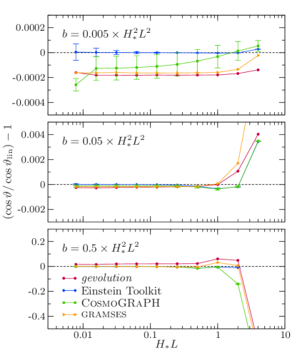
Figure 2 shows results for the observable (17) as computed from the different codes, relative to the linear solution (21), i.e. $({\rm cos}\vartheta/{\rm cos}\vartheta_{\rm lin})-1$, as a function of the dimensionless product $H_{*}L$; the length scale of the perturbation in units of the Hubble scale. Panels, top to bottom, show three different sets of initial perturbation amplitudes, $b\in\{0.005,0.05,0.5\}\times H_{\ast}^{2}L^{2}$, respectively. Red circles show the results from gevolution, blue diamonds show the results from the ET, green squares show the results from CosmoGRaPH, and orange triangles show the results from gramses, with dashed lines showing the linear solution for reference. Data and corresponding error bars for ET and CosmoGRaPH  were calculated using a Richardson Extrapolation, i.e. the data points shown represent values extrapolated to $N\rightarrow\infty$, see Appendix B for details.

In gevolution, the weak-field approximation includes all terms in the expansion up to $\mathcal{O}(b)$, and so for large perturbations (and for $H_{\ast}L\gtrsim 1$) we do expect to see a difference with respect to the ET and CosmoGRaPH. A similar statement can be made about gramses, which, due to the conformal flatness approximation, neglects tensor modes that might be excited during the evolution of the system at $\mathcal{O}(b^{2})$ and beyond.

The top panel of Figure 2 shows results for the smallest-amplitude perturbation, i.e. $b=0.005\times H_{*}^{2}L^{2}$. For this case we see agreement with the linear solution to within $0.03\%$ for all codes and for all values of $H_{*}L$. The ET provides the most numerically accurate solution in this regime where the perturbations remain linear. In this case, the fluid description implemented in the ET remains valid, which carries a smaller numerical error because it does not require smoothing over a particle distribution at each time step. To within numerical accuracy of the simulations performed, the only resolvable effect is a $0.003\%$ deviation from the linear solution for the ET with $H_{*}L=4$ – with the exception of one outlying CosmoGRaPH point at the smallest $L$ and $b$ due to poor numerical convergence, discussed further in Appendix B.

Especially at large values of $H_{*}L$ the performance of the linear prediction may seem surprising, but can be understood from the following considerations. First, working in Poisson gauge where the vector perturbation is in the shift, we can see that the linear expression for the shift is in fact exact on the initial hypersurface, cf. eqs. (16) and (19). The shift also appears only linearly in the geodesic equation (see Appendix D), and the terms due to the lapse perturbation, which is formally $\mathcal{O}(b^{2})$ outside of the initial hypersurface, would alone not lead to a deflection in the considered setup due to symmetry. Hence their effect appears only at one order higher, namely $\mathcal{O}(b^{3})$. There are no new $\mathcal{O}(b^{2})$ corrections as one moves away from the initial hypersurface because the matter dynamics are mainly due to inertia.

Considering the perturbations $b=0.05\times H_{*}^{2}L^{2}$, shown in the middle panel of Figure 2, we see measurable deviation from the linear solution for values of $H_{*}L\gtrsim 1$. These are below $\sim 1\%$ in all codes, and the numerical relativity codes ET and CosmoGRaPH  agree within their quoted numerical accuracy. The results from gevolution  and gramses show a qualitatively similar deviation from the linear prediction, and are well within expected truncation errors from higher-order terms of $\mathcal{O}(b^{2})$ (i.e. quadratic in the shift or higher, see Section IV.1) in the weak-field expansion. However, in the case of gramses  the roughly constant deviation from the linear solution for $H_{*}L\lesssim 1$ is a result of the mesh discretization error (see Section IV.2).

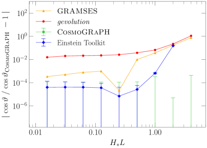
In the most extreme case with $b=0.5\times H_{*}^{2}L^{2}$ — close to the limit set by the weak energy condition — shown in the bottom panel of Figure 2, we see the strongest deviations from the linear prediction. Incidentally, the linear prediction still holds to a good approximation for $H_{*}L\leq 1$, as confirmed by all four codes. In this regime, gevolution shows a persistent $\sim 2\%$ error which is consistent with dropping terms of order $B_{i}\partial^{2}B_{i}{\sim b^{2}/L^{2}}$ from Einstein’s equations: compared to terms linear in $B_{i}$ their relative amplitude is indeed $\sim b/(H_{\ast}L)^{2}$ in some cases. The difference between gevolution  and the other three codes for all values of $H_{*}L$, is therefore still well within the expected $\mathcal{O}(b^{2})$ truncation error from the weak-field expansion. We have clipped the points for $H_{*}L=4$ in the bottom panel of Figure 2 to ensure deviations at smaller $H_{*}L$ can be resolved. In this case, we find deviation from the linear solution for gevolution  of $-0.619$, for gramses  of $-0.68$, and for CosmoGRaPH  of $-0.8183\pm 0.0004$. For the ET simulation with $H_{*}L=4$, we could not find a null geodesic that connects either event A or B with the observer, possibly indicating the presence of a horizon. We suggest this is a result of the fluid approximation used in the ET, since all other codes use a particle description and do not have this issue.

To highlight the difference between codes in the extreme regime shown in the bottom panel of Figure 2, we also plot the observable (17) from each code relative to that calculated in CosmoGRaPH  in Figure 3. Here we see gevolution  and gramses  agree to within $\sim 1\%$ and $\lesssim 0.1\%$ for small values of $H_{*}L$, respectively. This difference grows to $\sim 1$ for the largest box size $H_{*}L=4$. For $H_{*}L<1$ the ET and CosmoGRaPH agree within their numerical errors, however at $H_{*}L=1$ we see a small deviation, which increases to $\sim 15\%$ for $H_{*}L=2$. In this case we expect stream crossing has occurred; a regime in which we no longer trust the fluid approximation implemented in the ET, and the $N$-body (Vlasov) description used in CosmoGRaPH  is more physically relevant. However, the fluid approximation is more numerically accurate than $N$-body per computational cost, as can be seen clearly in the top panel of Figure 2. This is due to the additional numerical error introduced by smoothing over the particle distribution at each time step in order to source the metric evolution, see e.g. Giblin et al. (2019a). Regardless, the inability of the fluid approximation to capture stream crossings implies that once these occur, the results from the ET should not necessarily be considered representative of collisionless matter.

Figure 3: Relative difference between the observable (17) measured in each code and that measured in CosmoGRaPH  for simulations with $b=0.5\times H_{*}^{2}L^{2}$. We use CosmoGRaPH  as a reference here as we expect it to produce the most reliable results in this extreme case. Red circles show residuals for gevolution, orange triangles for gramses, and blue diamonds for the Einstein Toolkit. Green lines show the error bars from the CosmoGRaPH  results.

VI Conclusions

In this work we have compared the computational approaches of four independent, relativistic, cosmological simulation codes. Specifically, we studied a coordinate-invariant effect on null geodesics that is produced by an artificially strong gravitomagnetic field. In the process we have also explored the validity of the linear approximation for the frame-dragging effect.

We summarize our main findings as follows:

• For perturbations with amplitude $b=0.005\times H_{*}^{2}L^{2}$, we find a match to linear theory within 0.03% for all codes and for all box sizes studied here.

• For larger perturbations, with amplitudes $b\in\{0.05,0.5\}\times H_{*}^{2}L^{2}$, we find agreement with linear theory within 0.1% and 1%, respectively, for all sub-horizon box sizes $H_{\ast}L\lesssim 1$. However, gevolution has a persistent deviation of almost 2% for the highest perturbation amplitude, which is nonetheless consistent with its approximation scheme.

• In CosmoGRaPH, the deviation from linear theory is $\sim 80\%$ for $H_{*}L=4$ and $b=0.5\times H_{*}^{2}L^{2}$. We expect CosmoGRaPH  to provide the most trustworthy results in this extreme case; a regime in which $\gtrsim\mathcal{O}(b^{2})$ effects are relevant and stream crossing occurs.

• The weak-field approximation used in gevolution  agrees well with the numerical relativity codes for most cases studied here. Any deviations seen are well within the expected $\mathcal{O}(b^{2})$ for all choices of parameters. Due to the fact that Einstein’s equations are second order, some of these corrections can scale as $\sim b^{2}/L^{2}$, which means that they survive even in the sub-horizon limit.

• In gramses, deviations from the linear solution in cases well into the linear regime are dominated by the mesh discretization error, while for larger perturbations deviations from other codes are mainly due to the conformal flatness approximation, and are within the expected $\mathcal{O}(b^{2})$ truncation error.

• We find agreement within numerical uncertainties between the numerical relativity codes, ET and CosmoGRaPH, in most cases. Exceptions are those in which stream crossing occurs, at which point the fluid description used in ET is no longer resolving the full phase-space dynamics, and CosmoGRaPH  provides a more physically relevant result.

The test performed here is unique in that it is applicable only to codes which consider general-relativistic effects. Each code has differences in either its approximation of GR and/or numerical method. This study therefore provides an important test of these approximations and their limits in describing nonlinear dynamics.

A number of other relativistic effects would of course be interesting to investigate using these codes. These include, but are not limited to, studying in detail the collapse and virialisation of structures, the development and relevance of local spatial and Weyl curvature (electric vs. magnetic), coupling between small scales — where the matter distribution is very nonlinear — and the largest sub-horizon scales, gravitational waves, and the impact that any of these effects may have on current and future cosmological observations.

The codes used here each have their limitations, e.g. ET is currently limited to a fluid description of matter, and therefore cannot be used to study virialisation, while gramses uses the conformal flatness approximation and therefore cannot be used to study gravitational waves. Comparing our codes in regimes where such effects may be relevant therefore is beyond the scope of this paper. Nonetheless, we further emphasise that by inducing a strong gravitomagnetic field, we have considered a regime where all relativistic degrees of freedom are excited once nonlinearity becomes relevant. While we leave the investigation of other relativistic effects to future studies, it seems reasonable to expect that these will not contradict the results we found here.

Appendix A Constraint violation in NR codes

Here we analyse the constraint violation for the numerical relativity codes ET and CosmoGRaPH  for two select simulation cases. These codes are based upon hyperbolic formulations of Einstein’s equations, which evolve the dynamical equations but do not explicitly enforce the constraint equations. The constraints (7) and (8) are instead used as a diagnostic tool to check whether solutions have drifted too far from the physical constraint surfaces, i.e. to determine how well energy and momentum have been conserved in a general-relativistic sense.

Although this check is a good diagnostic, it does not necessarily imply validity of solutions, as numerical error can violate the dynamical evolution equations while still preserving constraints. For a timestep sufficiently small that the error in the dynamical evolution is small, remaining error will be dominated by truncation error when evolving vacuum or fluid solutions, or particle noise in the N-body case. In both cases, we can compute the rate at which the constraint violation in simulations converges to zero, and compare this to theoretical expectations.

In the case of stream-crossings, or caustics, it has been found that the constraint violation in the vicinity of a caustic will not converge in general Giblin et al. (2019a); East (2019). This is due to the presence of a mild singularity in the vicinity of caustics, where curvature scalars can diverge, yet the metric remains in a weak-field limit and the spacetime is geodesically complete. In the N-body case, we therefore expect constraint violation to be well-behaved before stream-crossings, and poor after. We expect the constraint violation to be well-behaved at all times in the corresponding fluid limit (assuming all relevant scales are resolved, i.e. that all gradients in the fluid remain constant between resolutions).

Figure 4: Hamiltonian constraint violation for the ET (blue) and CosmoGRaPH  (green), for $H_{*}L=0.0625$ (top panel) and $H_{*}L=2$ (bottom panel). Both panels show simulations with amplitude $b=0.5\times H_{*}^{2}L^{2}$. Solid curves show the highest resolution, dashed curves the medium resolution, and dotted curves the lowest resolution. Here we show the L2 norm (23) of the constraint violation as a function of approximate simulation scale factor.

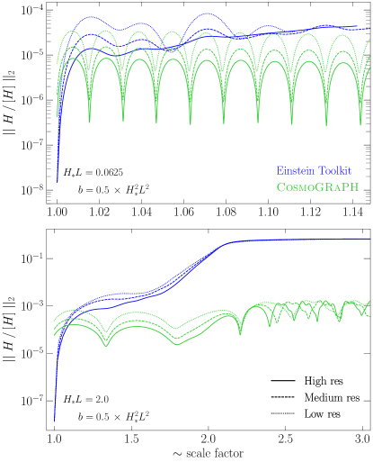
In Figure 4 we show the constraint violation as a function of approximate scale factor of the simulation, for ET (blue curves) and CosmoGRaPH  (green curves). We use the volume of the entire simulation domain, $V_{\mathcal{D}}$, to calculate the approximate scale factor, i.e.,

$$a_{\mathcal{D}}(t)=\left(\frac{V_{\mathcal{D}}(t)}{V_{\mathcal{D}}(t_{\rm init})}\right)^{1/3},$$ (22)

where $V_{\mathcal{D}}\equiv\int_{\mathcal{D}}\sqrt{\gamma}\,d^{3}X$, and $\gamma$ is the determinant of the spatial metric $\gamma_{ij}$.

The top panel of Figure 4 shows the simulation with $H_{*}L=0.0625$, and the bottom panel shows $H_{*}L=2$. Both simulations shown here have perturbation amplitude $b=0.5\times H_{*}^{2}L^{2}$. Solid curves show the highest resolution, dashed curves the medium resolution, and dotted curves the lowest resolution. These sets of resolutions differ slightly between ET and CosmoGRaPH, see Sections IV.3 and IV.4, respectively, for details. Specifically, Figure 4 shows the L2 error of the normalised Hamiltonian constraint violation, i.e.,

$$||H/[H]||_{2}=\frac{\sqrt{\sum_{i}H_{i}^{2}}}{\sqrt{\sum_{i}[H]_{i}^{2}}},$$ (23)

where $H_{i}$ is the Hamiltonian constraint violation at grid cell $i$ (for an exact solution we have $H_{i}=0$ everywhere), and the normalisation is

$$[H]\equiv\sqrt{\left({}^{3}R\right)^{2}+\left(K^{2}\right)^{2}+\left(K_{ij}K^{ij}\right)^{2}+\left(16\pi G\rho\right)^{2}},$$ (24)

where $\rho=\alpha^{2}\rho_{0}(u^{0})^{2}$ is the mass-energy density on the simulation hypersurfaces (not necessarily the rest-frame of the matter), and $[H]_{i}$ is (24) evaluated at grid cell $i$.

For the smaller box size, in the top panel of Figure 4, both simulations show convergence of the L2 error with an increase in resolution. For the larger box size $H_{*}L=2$ in the bottom panel of Figure 4, the perturbation has more time to grow in a few light-crossing times of the box. For the N-body approach used in CosmoGRaPH, convergence is found up until a stream-crossing occurs, at a scale factor of $a\sim 2$. After this time, inexact cancellation of numerically large (and formally infinite) contributions to the Hamiltonian constraint leads to a lack of convergence of constraint violation. For ET we see convergence until approximately the same time as CosmoGRaPH  in this case, after which the constraint violation is approximately the same at all resolutions, and reaches order unity. For this particular simulation, gradients are no longer consistent between resolutions and so we do not expect convergence of the constraints in general. After stream crossing, we do not expect the fluid approach used by ET to be representative of collisionless matter. While convergence of the constraints diverges due to caustic formation, convergence of the metric itself and its first derivatives is still found, leading to convergent results for the observable as discussed in the next section.

Appendix B Convergence and errors

B.1 Numerical convergence of observable

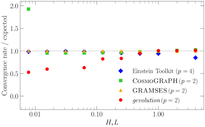
Here we check numerical convergence of the observable presented in Figure 2 as a function of resolution for all codes. We must ensure that our numerical calculations provide results with a sufficient degree of precision that they are meaningful, i.e. that they are approaching a continuum limit solution. We expect different rates of convergence for each code, due to different dominant error sources which depends on the numerical approximations made in each case.

We compute the convergence rate by evaluating the observable at three different resolutions, $\Delta x_{1}$, $\Delta x_{2}$, and $\Delta x_{3}$. For a method of order $p$, the error will be $\mathcal{O}(\Delta x^{p})$, and the convergence rate of the observable angle $\vartheta$ is given by

$$\mathcal{C}=\frac{\vartheta_{\Delta x_{1}}-\vartheta_{\Delta x_{2}}}{\vartheta_{\Delta x_{2}}-\vartheta_{\Delta x_{3}}},$$ (25)

and the theoretical convergence rate is

$$\mathcal{C}_{\rm expected}=\frac{\Delta x_{1}^{p}-\Delta x_{2}^{p}}{\Delta x_{2}^{p}-\Delta x_{3}^{p}}\,.$$ (26)

Figure 5 shows the convergence rate relative to the theoretical convergence rate for each code, for the set of simulations in the top panel of Figure 2. The expected convergence rate is calculated using (26) and the order of the integration scheme implemented in each code, $p$, as indicated in the legend. For this small perturbation, we expect all results to match the linear solution to a good approximation, and so it is an ideal case in which to test numerical convergence (although we have confirmed convergence for larger $b$ as well). From Figure 5 we see all codes give close to their expected numerical convergence rate for all values of $H_{*}L$. In gevolution we see a drop to first-order convergence inside the horizon. This is possibly due to the fact that we are approaching a quasistatic limit in which the error in the time integrator becomes subdominant. The elliptic constraint for the gravitomagnetic potential is solved by inverting a first-order finite-difference Laplacian, which may become the dominant source of error in this regime. We note a few peculiar convergence values in Figure 5 for CosmoGRaPH, gevolution, and ET, at $H_{*}L=0.0078125,0.03125,$ and $2$, respectively. In the case of CosmoGRaPH, we believe this is due to truncation error surpassing error introduced from particle noise, leading to a different convergence rate than expected, and thus effective method order $p$; this additionally results in a poorly extrapolated data point and error bar as seen in Figure 2. The remaining simulations appear to show normal numerical convergence for, e.g., the constraint violation in the case of ET, and so we believe the simulations themselves are providing reliable results. We therefore suggest that the non-convergence of the observable is related to the root-finding algorithm implemented in the ray tracing code used, but we do not investigate this further since all other points show good convergence.

Figure 5: Convergence rate (25) for the observable (17) calculated in simulations with $b=0.005\times H_{*}^{2}L^{2}$. We show the convergence rate relative to its expected value (26), for the Einstein Toolkit (blue diamonds), CosmoGRaPH (green squares), gramses (orange triangles), and gevolution (red circles).The order of the integration scheme, $p$, implemented in each code is indicated in the legend.

B.2 Error calculation

For ET and CosmoGRaPH, simulations were run at three different spatial resolutions for each value of $b$ and $H_{*}L$. This allows us to quantify the numerical error on the observables we compute from these simulations, as well as to estimate values in the $N\rightarrow\infty$ limit using a Richardson extrapolation. The values and error bars are calculated by fitting curves consistent with the expected order of convergence of the scheme used, and extrapolating to find the continuum-limit solution. The numerical error bars shown in Figure 2 are computed using differences between numerical values and the extrapolated, continuum-limit solutions in the case of ET, and using the distribution of extrapolated values in the case of CosmoGRaPH.

Appendix C Initial conditions with BSSN variables

The BSSN conformal factor and extrinsic curvature trace are given by Shibata and Nakamura (1995); Baumgarte and Shapiro (1999)

$$\phi_{\ast}^{\rm BSSN} = 0$$ (27)

$$K_{\ast} = -3H_{\ast}\,.$$ (28)

Because the determinant of the spatial metric $\gamma^{*}=1$, the conformal BSSN metric is given by $\bar{\gamma}_{ij}^{\ast}=\gamma_{ij}^{*}$. The conformally related trace-free part of the extrinsic curvature is given by

$$\bar{A}_{ij}^{*}=3\begin{pmatrix}0&\frac{3b}{4L}\cos\frac{2\pi y}{L}&0\\ \frac{3b}{4L}\cos\frac{2\pi y}{L}&\frac{3b^{2}}{2H_{\ast}L^{2}}\cos^{2}\frac{2\pi y}{L}&0\\ 0&0&0\end{pmatrix}\,,$$ (29)

and the conformal, contracted Christoffel symbol is

$$\bar{\Gamma}^{i}_{\ast}=\left(\begin{array}[]{c}-\frac{2\pi b}{H_{\ast}L^{2}}\sin\frac{2\pi y}{L}\\ 0\\ 0\end{array}\right)\,.$$ (30)

Lastly, the 3+1/ADM density is given by

$$\rho^{*}_{\rm ADM}=\frac{3H_{*}^{2}}{8\pi{G}}-\frac{9b^{2}\cos^{2}\left(\frac{2\pi y}{L}\right)}{128\pi{G}L^{2}}\,,$$ (31)

and relativistic gamma factor $W_{\ast}=\alpha_{\ast}u_{\ast}^{0}$

$$W_{\ast}=\frac{16H_{*}^{2}L^{2}-3b^{2}\cos^{2}\left(\frac{2\pi y}{L}\right)}{\sqrt{\left(16H_{*}^{2}L^{2}-3b^{2}\cos^{2}\left(\frac{2\pi y}{L}\right)\right)^{2}-64\pi^{2}b^{2}\sin^{2}\left(\frac{2\pi y}{L}\right)}}$$ (32)

Appendix D Photon integration

The geodesic equations parallel transport velocity vectors in the direction of the velocity,

$$k^{\mu}\nabla_{\mu}k^{\nu}=0\,,$$ (33)

for a photon 4-vector $k^{\mu}$, or for ordinary matter with $k^{\mu}\rightarrow u^{\mu}$. In order to integrate this numerically, we can cast this expression into a 3+1 form conducive to numerical integration, and for which the effects of frame-dragging due to a nonzero shift are transparent,

$$\frac{dk_{i}}{dt} = -\alpha k^{0}\partial_{i}\alpha+k_{j}\partial_{i}\beta^{j}-\frac{1}{2k^{0}}k_{j}k_{k}\partial_{i}\gamma^{jk}$$

$$\frac{dx^{i}}{dt} = \gamma^{ij}\frac{k_{j}}{k^{0}}-\beta^{i}\,.$$ (34)

Lastly, the observable, eq. (17), can be rewritten without a reference to basis vectors for an observer at rest, $u^{\mu}\propto(1,\vec{0})$, as

$$\cos\vartheta=\left.\frac{\gamma^{ij}k_{i}^{A}k_{j}^{B}}{\sqrt{\gamma^{ij}k_{i}^{A}k_{j}^{A}}\sqrt{\gamma^{ij}k_{i}^{B}k_{j}^{B}}}\right|_{O}\,,$$ (35)

provided the vectors are observed simultaneously. In order to obtain this simple expression we also used the fact that $\beta^{i}$ vanishes at our observer location due to symmetry. For non-simultaneous arrivals, one vector will need to be parallel transported along the observer’s trajectory. The parallel transport equation can be written

$$u^{\mu}\nabla_{\mu}k^{\nu} = 0$$

$$\rightarrow\frac{dk_{i}}{dt} = -\alpha k^{0}\partial_{i}\alpha+k_{j}\partial_{i}\beta^{j}-\frac{1}{2u^{0}}u_{l}k_{j}\partial_{i}\gamma^{lj}$$ (36)

$$+\alpha\left(\frac{u_{k}}{u^{0}}k^{0}-k_{k}\right)K_{i}^{k}\,,$$

where the last term here is new compared to eq. (D), and the second-last term now is sensitive to the observer’s velocity. In terms of $3+1$ variables, and for the metric and observer considered in this work, and for a gauge choice that respects symmetry of the problem (so $\partial_{i}\alpha=0$ at $y=0$), this expression simplifies to

$$\frac{dk_{i}}{dt}=k_{j}\partial_{i}\beta^{j}-\alpha k_{j}K^{j}_{i}\,,$$ (37)

which is integrated purely in time at $y=0$. The observable, eq. (35), is also evaluated using the metric at the time the second ray arrives.