Realistic Re-evaluation of Knowledge Graph Completion Methods: An Experimental Study

Abstract.

In the active research area of employing embedding models for knowledge graph completion, particularly for the task of link prediction, most prior studies used two benchmark datasets FB15k and WN18 in evaluating such models. Most triples in these and other datasets in such studies belong to reverse and duplicate relations which exhibit high data redundancy due to semantic duplication, correlation or data incompleteness. This is a case of excessive data leakage—a model is trained using features that otherwise would not be available when the model needs to be applied for real prediction. There are also Cartesian product relations for which every triple formed by the Cartesian product of applicable subjects and objects is a true fact. Link prediction on the aforementioned relations is easy and can be achieved with even better accuracy using straightforward rules instead of sophisticated embedding models. A more fundamental defect of these models is that the link prediction scenario, given such data, is non-existent in the real-world. This paper is the first systematic study with the main objective of assessing the true effectiveness of embedding models when the unrealistic triples are removed. Our experiment results show these models are much less accurate than what we used to perceive. Their poor accuracy renders link prediction a task without truly effective automated solution. Hence, we call for re-investigation of possible effective approaches.

1. Introduction

Large-scale knowledge graphs such as Freebase (Bollacker et al., 2008), DBpedia (Auer et al., 2007), NELL (Carlson et al., 2010), Wikidata (Vrandečić and Krötzsch, 2014), and YAGO (Suchanek et al., 2008) store real-world facts as triples in the form of (head entity (subject), relation, tail entity (object)), denoted (h, r, t), e.g., (Ludvig van Beethoven, profession, Composer). They are an important resource for many AI applications, such as question answering (Yao and Van Durme, 2014; Yih et al., 2015; Xu et al., 2016), search (Eder, 2012), and smart healthcare (Rotmensch et al., 2017), to name just a few. Despite their large sizes, knowledge graphs are far from complete in most cases, which hampers their usefulness in these applications.

To address this important challenge, various methods have been proposed to automatically complete knowledge graphs. Existing methods in this active area of research can be categorized into two groups (Nickel et al., 2016). One group is based on latent feature models, also known as embedding models, including TransE (Bordes et al., 2013), RESCAL (Nickel et al., 2011), and many other methods (Cai et al., 2018). The other group is based on observed feature models that exploit observable properties of a knowledge graph. Examples of such methods include rule mining systems (Galárraga et al., 2013) and path ranking algorithms (Lao and Cohen, 2010).

Particularly, the latent feature models are extensively studied. They embed each entity h (or t) into a multi-dimensional vector h (or t). A relation $r$ can have different representations. For example, in RESACL (Nickel et al., 2011), each relation is a weight matrix whose entries specify the interaction of latent features. In TransE (Bordes et al., 2013), a relation is a vector r that represents a geometric transformation between the head and tail entities in the embedding space and embeddings are learned in such a way that, if (h, r, t) holds, then $\textbf{h}+\textbf{r}\approx\textbf{t}$.

Embedding models have been extensively evaluated on link prediction, a task that predicts the missing h in triple (?, r, t) or missing t in (h, r, ?). Two benchmark datasets FB15k (a subset of Freebase) and WN18 (extracted from WordNet (Miller, 1995)), created by Bordes et al. (Bordes et al., 2013), are almost always used in such evaluation. Toutanova and Chen (Toutanova and Chen, 2015) noted that FB15k contains many reverse triples, i.e., it includes many pairs of (h, r, t) and (t, r^-1, h) where r and r^-1 are reverse relations. They constructed another dataset, FB15k-237, by only keeping one relation out of any pair of reverse relations. Similarly, Dettmers et al. (Dettmers et al., 2018) created WN18RR out of WN18 by removing reverse triples. The community has started to use FB15k-237 and WN18RR in evaluating models and noted significant performance degeneration of existing models in comparison with their performance on FB15k and WN18 (Dettmers et al., 2018; Toutanova and Chen, 2015; Akrami et al., 2018).

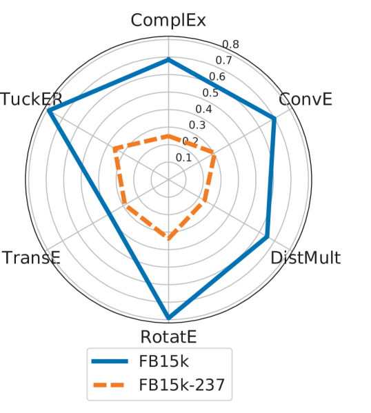
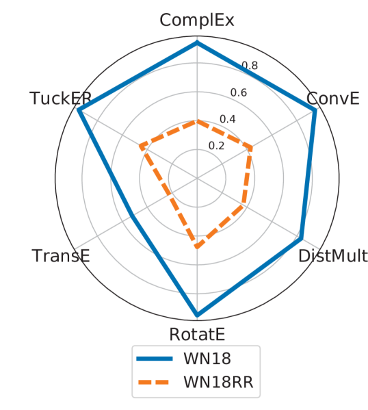
Figure 1. Performance of embedding models on FB15k vs. FB15k-237 and WN18 vs. WN18RR using FMRR^↑

Impact of reverse relations:   This paper thoroughly examines the impact of reverse triples in FB15k and WN18 (details in Section 4.2.1). The idiosyncrasies of the link prediction task on such data can be summarized as follows. A1) Link prediction becomes much easier on a triple if its reverse triple is available. A2) For reverse triples, a straightforward method could be even more effective than complex machine learning models. We discovered that 70% of the triples in the training set of FB15k form reverse pairs. Similarly, for 70% of the triples in its test set, reverse triples exist in the training set. For WN18, these two percentages are even higher—92.5% and 93%. The abundant reverse triples suggest that embedding models would have been biased toward learning whether two relations r₁ and r₂ form a reverse pair. Instead of complex models, one may achieve this goal by using statistics of the triples to derive simple rules of the form (h, r₁, t) $\Rightarrow$ (t, r₂, h). In fact, we generated such a simple model which attained 71.6% for FB15k and 96.4% for WN18 using FHits@1^↑, a common accuracy measure for embedding models.  These results are on par with those by the best performing embedding models—73.8% and 94.6% on FB15K and WN18, respectively, as can be seen from Table 13 in Section 5.

The above analysis suggests that the reverse triples led to a substantial over-estimation of the embedding models’ accuracy, which is verified by our experiments on a wide range of models. While Section 5 examines the results in detail, Figure 1 illustrates the performance comparison of a few representative models using another popular measure FMRR^↑. The results show that R1) the performance of all existing embedding models degenerates significantly after reverse triples are removed. R2) Many successors of the original TransE model were empirically shown to outperform TransE by far on FB15k, but they only attained similar or even worse performance on FB15k-237. For example, the FHits@10^↑ of ComplEX vs. TransE is 42.3% vs. 47.5% on FB15k-237, in stark contrast to 83.2% vs. 62.4% on FB15k. R3) The absolute accuracy of all models is poor, rendering them ineffective for real-world link prediction task. For example, TuckER (Balažević et al., 2019) attains the best FMRR^↑ on FB15k-237 (0.355). However, its performance on FB15k (0.79) was considerably stronger. Similarly, RotatE (Sun et al., 2019) has 0.95 FMRR^↑ on WN18 but only 0.476 on WN18RR.

The existence of excessive reverse triples in FB15k and WN18—the de facto benchmark datasets for link prediction—actually presents a more fundamental defect in many of these models: A3) the link prediction scenario, given such data, is non-existent in the real-world at all. With regard to FB15k, the redundant reverse relations, coming from Freebase, were just artificially created. When a new fact was added into Freebase, it would be added as a pair of reverse triples, denoted explicitly by a special relation reverse_property (Pellissier Tanon et al., 2016; Färber, 2017). In WN18, 17 out of the 18 relations are reverse relations. Some are reverse of each other, e.g., hypernym and hyponym—flower is a hypernym of sunflower and sunflower is a hyponym of flower. Others are self-reciprocal, i.e., symmetric relations such as verb_group—(begin, verb_group, start) and (start, verb_group, begin) are both valid triples. For such intrinsically reverse relations that always come in pair when the triples are curated into the datasets, there is not a scenario in which one needs to predict a triple while its reverse is already in the knowledge graph. Training a knowledge graph completion model using FB15k and WN18 is thus a form of overfitting in that the learned model is optimized for the reverse triples which cannot be generalized to realistic settings. More precisely, this is a case of excessive data leakage—the model is trained using features that otherwise would not be available when the model needs to be applied for real prediction. There could be more natural reverse triples that are worth prediction—two relations are not semantically reverse but correlate and/or the reverse triples are not available together in the knowledge graph due to how the data are collected. We discuss such cases of data redundancy below.

Impact of other data redundancy and Cartesian product relations:   The data leakage due to reverse triples is a form of data redundancy that unrealistically inflates the models’ accuracy. We identified other types of data redundancy in FB15k and another evaluation dataset YAGO3-10 (Section 4.2.2). Specifically, some relations are duplicate as their subject-object pairs substantially overlap, and some are reverse duplicate when one relation’s subject-object pairs overlap a lot with another relation’s object-subject pairs.

We also discovered another type of relations, which we call Cartesian product relations (Section 4.3), that unrealistically inflate a model’s accuracy. Given such a relation, there are a set of subjects and a set of objects, and the relation is valid from every subject in the first set to every object in the second set. In a May 2013 snapshot of Freebase, close to 10% of the relations are Cartesian product relations. In FB15k, 142 out of the 1345 relations are such relations. One example is position, since every team in a certain professional sports league has the same set of positions. The link prediction problem for such relations thus becomes predicting, say, whether an NFL team has the quarter-back position, which is not very meaningful in the real-world. Moreover, when a substantial subset of the aforementioned subject-object Cartesian product is available in the training set, it is relatively easy for a model to attain a strong prediction accuracy.

The same analyses A1-A3 on reverse relations are also applicable on duplicate and Cartersian product relations, and the same observations R1-R3 can be made from our experiment results. A1) In evaluating prediction models, it is misleading to mix such straightforward relations with more realistic, challenging relations. In the test set of FB15k, the numbers of reverse relations, duplicate and reverse duplicate relations, Cartesian product relations, and the remaining relations are 798, 118, 78, and 106, respectively. The FMRR^↑ of ConvE on such relations is 0.72, 0.948, 0.881, and 0.444, respectively. Another example is YAGO3-10 which has two largely duplicate relations isAffiliatedTo and playsFor that account for more than 63% of its test set. The FMRR^↑ of RotatE (Sun et al., 2019) is 0.612 on these 2 relations but only 0.304 on other relations. A2) Instead of learning complex embedding models, a simpler approach can be more effective. For duplicate and reverse duplicate relations, a simple rule based on data statistics can already be quite accurate, as similarly in the aforementioned case of reverse relations. For Cartesian product relations, by observing that a large percentage of possible subject-object pairs in a relation exist in the dataset, one can derive the relation is a Cartesian product relation and thus the same relation should exist in all such pairs. Our experiments on 9 Cartesian product relations in FB15k obtained an average FHits@10^↑ of 98.3% using this method, which is higher than the 96.3% FHits@10^↑ of TransE on these relations. A3) The existence of Cartesian product relations in FB15k is quite artificial. In fact, 60% of them are due to special “mediator nodes” in Freebase that represent multiary relationships and simplification in FB15k for removing such nodes through concatenating edges. Similarly, a vast majority of the duplicate and reverse duplicate relations in FB15k were artificially created. The dataset has 84 pairs of duplicate relations. In 80 out of the 84 pairs, one or both relations are concatenated. The numbers are 63 out of 67 pairs for reverse duplicate relations. Just like reverse triples, they render a link prediction scenario largely nonexistent in the real-world and lead to unrealistically strong prediction accuracy.

The much weaker performance of embedding models on FB15k-237 and WN18RR also drove us to examine observed feature models, specifically using rules discovered by the rule mining system AMIE (Galárraga et al., 2013). Our experiment results show that it also degenerates significantly on the more realistic FB15k-237 and WN18RR. Its FMRR^↑ on FB15k vs. FB15k-237 is 0.797 vs. 0.308 and is 0.94 vs. 0.357 on WN18 vs. WN18RR.

The embedding models generate a ranked list of candidate predictions which can be as long as the number of entities in a knowledge graph. For this ranked list to effectively assist human curators in completing the knowledge graph, the correct predictions should be ranked high. From this perspective, this study depicts a realistic picture of existing methods being much less accurate than one may perceive. As mentioned in R3, their absolute accuracy is poor, which renders link prediction a task without truly effective automated solution. Hence, we call for re-investigation of possible effective approaches for completing knowledge graphs.

This paper presents a systematic study with the main objective of assessing the true effectiveness of link prediction methods in real-world settings. Other studies continue to evaluate models using both FB15k and FB15k-237 (similarly WN18 and WN18RR), merely viewing the latter as a more challenging dataset. However, based on our analyses A1-A3 and experiment results R1-R3, we argue that FB15k and WN18 are completely misleading and should not be used anymore. Similarly, our results show that YAGO3-10, which has been recently used in some studies (Dettmers et al., 2018), also suffers from the same defect since the majority of its triples are duplicates.

A preliminary report of our study was in (Akrami et al., 2018), which presents much less comprehensive analyses and results. Other related studies are (Wang et al., 2019; Meilicke et al., 2018). The focus in (Wang et al., 2019), different from ours, is about how existing evaluation methods are more suitable for question answering than link prediction. Meilicke et al. (Meilicke et al., 2018) analyzed the types of rules that help knowledge graph completion by categorizing test triples of datasets based on explanations generated by their rule-based approach. The test leakage problem was also mentioned in (Dettmers et al., 2018), although their focus was to propose a new embedding model.

To sum up, this paper makes these contributions:

• It provides a thorough investigation of the data redundancy problem in how existing embedding models for knowledge graph completion were trained, due to reverse and duplicate triples in the de facto benchmark datasets FB15k and WN18 (Section 4).

• For the first time, it identifies the existence of Cartesian product relations in FB15k which, together with the data redundancy problem, makes previous performance measures of embedding models unrealistic (Section 4).

• It presents the results of a comprehensive evaluation of these defects’ impacts on the performance of many representative embedding models as well as an observed feature model AMIE (Section 5).

• All codes, experiment scripts, datasets, and results are in a public repository https://github.com/idirlab/kgcompletion. It will help ensure the reproducibility of this research.

2. Background: Knowledge Graph Completion Methods

This section briefly summarizes representative knowledge graph completion methods. In our description, vectors are represented as bold lower case letters such as x. $[\textbf{x}]_{i}$ represents the $i$th element of x. A matrix is denoted by a bold upper case letter, e.g., M. A knowledge graph $\mathcal{G}$ consists of a set of entities $\mathcal{E}$ and a set of relations $\mathcal{R}$. Triples are represented as (h, r, t) where h, t $\in\mathcal{E}$ are the head and tail entities, and relationship r $\in\mathcal{R}$ exists from the head to the tail. $\langle\textbf{x},\textbf{y},\textbf{z}\rangle=\sum_{i}[\textbf{x}]_{i}.[\textbf{y}]_{i}.[\textbf{z}]_{i}$ is the component-wise multi-linear dot product.

2.1. Latent Feature Models

Embedding-based methods employ two crucial components: (1) a scoring function to measure the plausibility of triples (h, r, t), and (2) a process to learn the representations (i.e., embeddings) of entities and relations by solving an optimization problem of maximizing the scores of correct triples while minimizing the scores of incorrect ones.

In TransE (Bordes et al., 2013), the scoring function is $f_{\textsl{\small r}}(\textsf{\small h},\textsf{\small t})=-\|\textbf{h}+\textbf{r}-\textbf{t}\|_{\ell_{1}/\ell_{2}}^{2}$. TransE is a scalable method with a small number of model parameters, but it has limitations in modeling $1$-to-$n$, $n$-to-$1$, and $m$-to-$n$ relations (Wang et al., 2014). TransH (Wang et al., 2014) aims to address TransE’s limitations by not using the same embedding of an entity in different relations.

Lin et al. (Lin et al., 2015b) proposed TransR which learns the embeddings in two different vector spaces $\mathbb{R}^{d}$ and $\mathbb{R}^{k}$ for entities and relations. They argued that using the same semantic space for entities and relations, as in TransE and TransH, is insufficient because they are two completely different types of objects. Instead, TransR defines a projection matrix $\textbf{M}_{r}$ to map entity embeddings to the vector space for each relation. In TransD (Ji et al., 2015), which improves over TransR, the projection matrix is decomposed to the product of two vectors. However, in contrast to TransR, there is a unique projection matrix for each entity-relation pair. RotatE (Sun et al., 2019) defines each relation as a rotation from the source entity to the target entity. The scoring function is $f_{\textsl{\small r}}(\textsf{\small h},\textsf{\small t})=-{\|\textbf{h}\circ\textbf{r}-\textbf{t}\|}^{2}$, where $\circ$ is the Hadmard (or element-wise) product.

To learn the entity and relation representations, a loss function is minimized. Two of the most-frequently used loss functions in embedding models are margin-based loss function $L=\sum_{(\textsf{\small h},\textsl{\small r},\textsf{\small t})\in S}\sum_{(\textsf{\small h'},\textsl{\small r},\textsf{\small t'})\in S^{\prime}}max(0,f_{\textsl{\small r}}(\textsf{\small h},\textsf{\small t})+\gamma-f_{\textsl{\small r}}(\textsf{\small h'},\textsf{\small t'}))$ and logistic loss $L=\sum_{(\textsf{\small h},\textsl{\small r},\textsf{\small t})\in S\cup S^{\prime}}log(1+exp(-y_{hrt}.f_{\textsl{\small r}}(\textsf{\small h},\textsf{\small t})))$. In the equations, $y_{hrt}$ is the sign of a training example (+1/-1 for positive/negative example), $\gamma$ is the margin, $S$ is the set of positive triples (h, r, t) in the training set and $S^{\prime}$ is the set of negative triples (h’, r, t’). Since a real-world knowledge graph contains only positive triples, negative triples in evaluation datasets were generated by corrupting the positive triples—a process that replaces the head or tail entity of each positive triple by other entities in the knowledge graph (Bordes et al., 2013).

Another approach formulates link prediction as a third-order binary tensor completion problem in which a knowledge graph is represented as a partially observed tensor $\textbf{Y}\in\{0,1\}^{|\mathcal{E}|\times|\mathcal{E}|\times|\mathcal{R}|}$. An entry in Y equals one if the corresponding triple exists in $\mathcal{G}$. Different models such as RESCAL (Nickel et al., 2011), DistMult (Yang et al., 2015), ComplEx (Trouillon et al., 2016), and TuckER (Balažević et al., 2019) used various methods of tensor factorization to decompose Y and assign scores to triples based on the learned factors. RESCAL is a collective matrix factorization model which represents a relation as a matrix $\textbf{W}_{r}\in\mathbb{R}^{d\times d}$ that describes the interactions between latent representations of entities. The score of a triple in this method is defined as $f_{\textsl{\small r}}(\textsf{\small h},\textsf{\small t})=\textbf{h}^{\top}\textbf{W}_{r}\textbf{t}$. DistMult is similar to RESCAL but it restricts relations to be diagonal matrices $\textbf{w}_{r}\in\mathbb{R}^{d}$ in order to reduce the number of relation parameters: $f_{\textsl{\small r}}(\textsf{\small h},\textsf{\small t})=\langle\textbf{h},\textbf{w}_{r},\textbf{t}\rangle$. Due to this simplification, DistMult can only model symmetric relations. ComplEx is an extension of DistMult. It uses complex numbers instead of real numbers to handle symmetric and anti-symmetric relations. TuckER is a model based on Tucker decomposition (Tucker et al., 1964) of Y. ConvE (Dettmers et al., 2018) is a neural network model that uses 2D convolutional layers over embeddings, and interactions between entities and relations are modeled by convolutional and fully connected layers.

2.2. Other Approaches

Unlike embedding models which employ latent features, observed feature models directly exploit observable features. For instance, by observing that most persons in a knowledge graph have the same citizenship as their parents, a system may possibly generate rule (a, is_citizen_of, c) $\wedge$ (a, has_child, b) $\Rightarrow$ (b, is_citizen_of, c), which can be also represented as is_citizen_of(a,c) $\wedge$ has_child(a,b) $\Rightarrow$ is_citizen_of(b,c). A representative of the observed feature models is the rule mining system AMIE (Galárraga et al., 2013). In AMIE, a rule has a body (antecedent) and a head (consequent), represented as $B_{1}\land B_{2}\land\ldots\land B_{n}\Rightarrow H$ or in simplified form $\overrightarrow{B}\Rightarrow H$. The body consists of multiple atoms $B_{1}$, $\ldots$, $B_{n}$ and the head $H$ itself is also an atom. In an atom r(h,t), which is another representation of fact triple (h, r, t), the subject and/or the object are variables to be instantiated. The prediction of the head can be carried out when all the body atoms can be instantiated in the knowledge graph.

The multi-hop link prediction approaches (Das et al., 2018; Lin et al., 2018) aim to find complex patterns in a knowledge graph by following reasoning paths, e.g., a$\to$$livesInCity$$\to$b$\to$$isInCountry$$\to$c. Given a query ($e$, r, ?), these approaches use reinforcement learning in learning to walk from $e$ to the answer entity by taking a labeled relation at each step, conditioned on the query relation and entire path history.

3. Existing Evaluation Framework

3.1. Evaluation Datasets

Table 1. Statistics of evaluation datasets

Dataset	#entities	#relations	#train	#valid	#test
FB15k	14,951	1,345	483,142	50,000	59,071
FB15k-237	14,541	237	272,115	17,535	20,046
WN18	40,943	18	141,442	5,000	5,000
WN18RR	40,943	11	86,835	3,034	3,134
YAGO3-10	123,182	37	1,079,040	5,000	5,000
YAGO3-10-DR	122,837	36	732,556	3,390	3,359

FB15k:

Most embedding models have been evaluated on FB15k, a subset of Freebase generated by Bordes et al. (Bordes et al., 2013). FB15k contains only those Freebase entities that were also available in Wikipedia based on the wiki-links database  and have at least 100 appearances in Freebase. The relations included into FB15k must also have at least 100 instances. 14,951 entities and 1,345 relations satisfy these criteria, which account for 592,213 triples included into FB15k. These triples were randomly split into training, validation and test sets. Table 1 shows the statistics of this and other datasets.

WN18:

Many embedding models have also been evaluated using WN18 (Bordes et al., 2013), a knowledge graph extracted from the English lexical database WordNet (Miller, 1995) which defines conceptual-semantic and lexical relations between word forms or between synsets—sets of synonyms. An example triple is (presentation, derivationally_related_form, present).

YAGO3-10:

Some embedding models were evaluated using YAGO3-10 (Dettmers et al., 2018), a subset of YAGO3 (Mahdisoltani et al., 2015)—the multilingual extension of YAGO (Suchanek et al., 2008) which is derived from Wikipedia and WordNet. YAGO3-10 contains entities that are involved in at least 10 relations in YAGO3.

3.2. Evaluation Methods and Measures

Embedding models have been evaluated using several highly-related knowledge graph completion tasks such as triple classification (Wang et al., 2014; Socher et al., 2013), link prediction (Lin et al., 2015a), relation extraction (Weston et al., 2013; Lin et al., 2015b), and relation prediction (Shi and Weninger, 2017). The link prediction task as described in (Bordes et al., 2013) is particularly widely used for evaluating different embedding methods. Its goal is to predict the missing h or t in a triple (h, r, t). For each test triple (h, r, t), the head entity h is replaced with every other entity $\textsf{\small h'}\in\mathcal{E}$ in the dataset, to form corrupted triples. The original test triple and its corresponding corrupted triples are ranked by their scores according to the score functions (Section 2.1) and the rank of the original test triple is denoted rank${}_{\textsf{\small h}}$. The same procedure is used to calculate rank${}_{\textsf{\small t}}$ for the tail entity t. A method with the ideal ranking function should rank the test triple at top.

The accuracy of different embedding models is measured using Hits@1^↑, Hits@10^↑, Mean Rank (MR^↓), and Mean Reciprocal Rank (MRR^↑), as in (Bordes et al., 2013). Hits@k^↑ is the percentage of top $k$ results that are correct. MR^↓ is the mean of the test triples’ ranks, defined as $MR=\frac{1}{2\ |T|}\sum_{(\textsf{\small h},\textsl{\small r},\textsf{\small t})\in T}(\emph{rank}_{\textsf{\small h}}+\emph{rank}_{\textsf{\small t}})$, in which $|T|$ is the size of the test set. MRR^↑ is the average inverse of harmonic mean of the test triples’ ranks, defined as $MRR=\frac{1}{2\ |T|}\sum_{(\textsf{\small h},\textsl{\small r},\textsf{\small t})\in T}(\frac{1}{\emph{rank}_{\textsf{\small h}}}+\frac{1}{\emph{rank}_{\textsf{\small t}}})$.

Besides these raw metrics, we also used their corresponding filtered metrics (Bordes et al., 2013), denoted FHits@1^↑, FHits@10^↑, FMR^↓, and FMRR^↑, respectively. In calculating these measures, corrupted triples that are already in training, test or validation sets do not participate in ranking. In this way, a model is not penalized for ranking other correct triples higher than a test triple. For example, consider the task of predicting tail entity. Suppose the test triple is (Tim Burton, film, Edward Scissorhands) and the training, test, or validation set also contains another triple (Tim Burton, film, Alice in Wonderland). If a model ranks Alice in Wonderland higher than Edward Scissorhands, the filtered metrics will remove this film from the ranked list so that the model would not be penalized for ranking (Tim Burton, film, Edward Scissorhands) lower than (Tim Burton, film, Alice in Wonderland), both correct triples.

We note that, by definition, higher Hits@1^↑ (FHits@1^↑), Hits@10^↑ (FHits@10^↑) and MRR^↑ (FMRR^↑), and lower MR^↓ (FMR^↓) indicate better accuracy.

4. Inadequacy of benchmarks and Evaluation Measures

In this section we investigate the existence and impact of a few types of relations in FB15k, WN18 and YAGO3-10, including reverse (and symmetric) relations, redundant relations, and Cartesian product relations. The outcome suggests that triples in these relations led to a substantial over-estimation of the accuracy of embedding models.

4.1. Identifying the Most Probable Freebase Snapshot Used for Producing FB15k

In order to understand the various defects in FB15k and their root cause, we searched for the same Freebase snapshot that was used to create FB15k. When it was active, Freebase maintained periodic snapshots, more frequent than monthly. It is unclear from (Bordes et al., 2013) which snapshot was used to create FB15k. To derive the most probable timestamp of the snapshot from which FB15k was produced, we compared the snapshots available at https://commondatastorage.googleapis.com/freebase-public/ as of June 2019. Particularly, we considered the snapshots in the several months before (Bordes et al., 2013) was published. We analyzed to what degree these snapshots overlap with FB15k.

The May 5, 2013 snapshot (i.e., https://commondatastorage.googleapis.com/freebase-public/rdf/freebase-rdf-2013-05-05-00-00.gz) has the largest overlap among these snapshots, as it contains 99.54% of the triples in FB15k. We thus concluded that FB15k was most likely drawn from a snapshot around May 5, 2013, which can be approximated by the snapshot on that exact date.

Mediator nodes, also called compound value type (CVT) nodes, are used in Freebase to represent multiary relationships. For example, Figure 2 shows several CVT nodes. The rightmost CVT node is connected to an award, two nominee nodes and a work through various relations. In the May 2013 Freebase snapshot, for many (but not all) CVT nodes, additional concatenated edges were created. Specifically, for such a CVT node, multiple triples were created, each a concatenation of two edges connected through the CVT node. These binary relationships partly capture the multiary relationship represented by the CVT node. For instance, the triples (Bafta Award For Best Film, award_category/nominees, CVT) and (CVT, award_nomination/nominated_for, A Room With A View) in Figure 2 would be concatenated to form a triple between the award and the work nominated for the award. The concatenation of two relations $\textsl{\small r}_{1}$ and $\textsl{\small r}_{2}$ is written as $\textsl{\small r}_{1}.\textsl{\small r}_{2}$. There are 54,541,700 concatenated triples in the May 2013 snapshot.

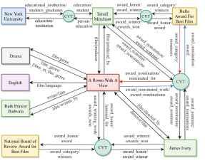
Figure 2. Mediator (CVT) nodes in Freebase

Concatenated Edges

FB15k does not include any CVT nodes or edges adjacent to such nodes from Freebase. However, it kept most concatenated edges (or maybe all, although we have no absolute way to verify, since nowhere we can find all Freebase snapshots that have ever been created). All the 707 concatenated relations in FB15k exist in the May 2013 snapshot. Among the 592,213 triples in FB15k, 396,148 are concatenated and 394,947 of them could be found in the snapshot.

4.2. Data Redundancy

4.2.1. Data Leakage Due to Reverse Triples

(1) FB15k: In (Toutanova and Chen, 2015), Toutanova and Chen noted that the widely-used benchmark dataset FB15k contains many reverse triples, i.e., it includes many pairs of (h, r, t) and (t, r^-1, h) where r^-1 is the reverse of r. Freebase actually denotes reverse relations explicitly using a special relation reverse_property. For instance, the triple (film/directed_by, reverse_property, director/film) in Freebase denotes that film/directed_by and director/film are reverse relations. Therefore, (A Room With A View, film/directed_by, James Ivory) and (James Ivory, director/film, A Room With A View) form a pair of reverse triples, as shown in Figure 2. The reverse relation of a concatenated relation $\textsl{\small r}_{1}.\textsl{\small r}_{2}$ is the concatenation of the corresponding reverse relations, i.e., $\textsl{\small r}_{2}^{-1}.\textsl{\small r}_{1}^{-1}$. For example, in Figure 2 award_nominated_work/award_nominations . award_nomination/award (blue edges) and award_category/nominees . award_nomination/nominated_for (red edges) are two concatenated relations which are reverse of each other.

Using the reverse relation information from the May 2013 snapshot of Freebase, out of the 483,142 triples in the training set of FB15k, 338,340 triples form 169,170 reverse pairs. Furthermore, for 41,529 out of the 59,071 triples (i.e., about 70.3%) in the test set of FB15k, their reverse triples exist in the training set. These data characteristics suggest that embedding models would have been biased toward learning reverse relations for link prediction. More specifically, the task can largely become inferring whether two relations r₁ and r₂ form a reverse pair. Given the abundant reverse triples in the dataset, this goal could potentially be achieved without using a machine learning approach based on complex embeddings of entities and relations. Instead, one may aim at deriving simple rules of the form (h, r₁, t) $\Rightarrow$ (t, r₂, h) using statistics about the triples in the dataset. In fact, Dettmers et al. (Dettmers et al., 2018) generated such a simple model which attained a 68.9% accuracy by the measure FHits@1^↑. We generated a similar model by finding the relations that have more then 80% intersections. It attained an FHits@1^↑ of 71.6%. This is even slightly better than the 70.3% accuracy one may achieve using an oracle based on the reverse relations denoted in the May 2013 Freebase snapshot. The FHits@1^↑ of the best performing embedding model on FB15k is 73.8% (more details in Table 13 of Section 5).

(2) WN18: WN18 also suffers from data leakage, as 14 out of its 18 relations form 7 pairs of reverse relations, e.g., (europe, has_part, republic_of_estonia) and (republic_of_estonia, part_of, europe) are two reverse triples in reverse relations has_part and part_of. There are also 3 self-reciprocal (i.e., symmetric) relations: verb_group, similar_to, derivationally_related_form. 4,658 out of the 5,000 test triples have their reverse triples available in the training set. The training set itself contains 130,791 (about 92.5%) triples that are reverse of each other. On WN18, we can achieve an FHits@1^↑of 96.4% by the aforementioned simple rule-based model (finding the relations that have more then 80% intersections) which is better than the results obtained by the embedding models (Table 13 of Section 5).

In training a knowledge graph completion model using FB15k and WN18, we fall into a form of overfitting in that the learned models are optimized for the reverse triples which cannot be generalized to realistic settings. More precisely, this is a case of excessive data leakage—the model is trained using features that otherwise would not be available when the model needs to be applied for real prediction.

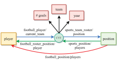
Figure 3. Duplicate relations

4.2.2. Other Redundant Triples

(1) FB15k: In addition to reverse relations, there are other types of semantically redundant relations in FB15k. While it is infeasible to manually verify such semantic redundancy, we used a simple method to automatically detect it. Given two relations $\textsl{\small r}_{1}$ and $\textsl{\small r}_{2}$, we calculate how much their subject-object pairs overlap. Suppose $|\textsl{\small r}|$ is the number of instance triples in relation r and $T_{\textsl{\small r}}$ denotes the set of subject-object pairs in r, i.e., $T_{\textsl{\small r}}=\{(\textsf{\small h},\textsf{\small t})\ |\ \textsl{\small r}(\textsf{\small h},\textsf{\small t})\in\mathcal{G}\}$. We say $\textsl{\small r}_{1}$ and $\textsl{\small r}_{2}$ are near-duplicate relations, simplified as duplicate relations, if they satisfy the following condition: $\frac{|T_{\textsl{\small r}_{1}}\cap T_{\textsl{\small r}_{2}}|}{|\textsl{\small r}_{1}|}>\theta_{1}$ and $\frac{|T_{\textsl{\small r}_{1}}\cap T_{\textsl{\small r}_{2}}|}{|\textsl{\small r}_{2}|}>\theta_{2}$. Moreover, $T_{\textsl{\small r}}^{-1}$ denotes the reverse entity pairs of $T_{\textsl{\small r}}$, i.e., $T_{\textsl{\small r}}^{-1}=\{(\textsf{\small t},\textsf{\small h})\ |\ (\textsf{\small h},\textsf{\small t})$ $\in$ $T_{\textsl{\small r}}\}$. We say $\textsl{\small r}_{1}$ and $\textsl{\small r}_{2}$ are reverse duplicate relations if they satisfy the following condition: $\frac{|T_{\textsl{\small r}_{1}}\cap T_{\textsl{\small r}_{2}}^{-1}|}{|\textsl{\small r}_{1}|}>\theta_{1}$ and $\frac{|T_{\textsl{\small r}_{1}}\cap T_{\textsl{\small r}_{2}}^{-1}|}{|\textsl{\small r}_{2}|}>\theta_{2}$. We have set $\theta_{1}$ and $\theta_{2}$ to 0.8 on FB15k.

For example football_position/players ($\textsl{\small r}_{1}$) and sports_position/players.football_roster_position/player ($\textsl{\small r}_{2}$) are duplicate based on this definition, since $\frac{|T_{\textsl{\small r}_{1}}\cap T_{\textsl{\small r}_{2}}|}{|\textsl{\small r}_{1}|}=0.87$ and $\frac{|T_{\textsl{\small r}_{1}}\cap T_{\textsl{\small r}_{2}}|}{|\textsl{\small r}_{2}|}=0.97$. These two relations are displayed in Figure 3 using red and green edges, respectively. The first relation records each football player’s position considering their overall career. For the second relation, each instance triple is a concatenation of two edges connected through a mediator node, representing a multiary relationship about the position a player plays for a team as shown in Figure 3. Since most players play at the same position throughout their careers, these two relations are redundant. Another example of similar nature is that $\textsl{\small r}_{1}$ and football_player/current_team . sports_team_roster/position ($\textsl{\small r}_{3}$) are reverse duplicate relations, because $\frac{|T_{\textsl{\small r}_{1}}\cap T_{\textsl{\small r}_{3}}^{-1}|}{|\textsl{\small r}_{1}|}=0.88$ and $\frac{|T_{\textsl{\small r}_{1}}\cap T_{\textsl{\small r}_{3}}^{-1}|}{|\textsl{\small r}_{3}|}=0.97$. In Figure 3 they are highlighted in red and blue, respectively.

For each test triple in FB15k, we use the methods explained to determine whether it has 1) reverse triples, 2) duplicate or reverse duplicate triples in the training set, and whether it has 3) reverse triples, 4) duplicate or reverse duplicate triples in the test set itself. A triple may have redundant triples in any of these four categories. We use bitmap encoding to represent different cases of redundancy. For example, 1100 is for a triple that has both reverse triples and (reverse) duplicate triples in the training set. Hence, there are 16 possible different combinatorial cases. Considering the test triples in FB15k, not all 16 cases exist. Instead, 12 different cases exist. Figure 4 shows the percentages of triples in different cases. The 7 cases smaller than 1% are combined in one slice. The largest three slices are 1000 (triples with only reverse triples in the training set), 0000 (triples without any redundant triples), and 0010 (triples with only reverse triples in the test set). In total, 41,529, 1,847 and 2,701 test triples have reverse, reverse duplicate and duplicate triples in the training set, and 4,992, 249, and 328 test triples have these categories of redundant triples in the test set itself. The data redundancy causes overestimation of embedding models’ accuracy. For instance, the FMR^↓, FHits@10^↑, FHits@1^↑, and FMRR^↑ of ConvE are 33.5, 88.8, 64.3, and 0.734 on such relations, whereas its performance using these measures on relations without any redundancy is only 149, 61.2, 37.3, and 0.454, respectively.

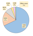
Figure 4. Redundancy in the test set of FB15k

(2) YAGO3-10: With 1,079,040 training triples, this dataset is larger than FB15k and WN18. However, among its 37 relations, the two most populated relations $\textsl{\small isAffiliatedTo}\ (r_{1})$ and $\textsl{\small playsFor}\ (r_{2})$ account for 35% and 30% of the training triples, respectively. Although $r_{1}$ semantically subsumes $r_{2}$ in the real world, they appear as near-duplicate relations in this particular dataset, as $\frac{|T_{\textsl{\small r}_{1}}\cap T_{\textsl{\small r}_{2}}|}{|\textsl{\small r}_{1}|}=0.75$ and $\frac{|T_{\textsl{\small r}_{1}}\cap T_{\textsl{\small r}_{2}}|}{|\textsl{\small r}_{2}|}=0.87$. In the training set, 557,696 triples find their duplicates in itself. 2,561 out of the 5,000 test triples have their duplicate triples available in the training set. The various models achieved much stronger results on $r_{1}$ and $r_{2}$ than other relations. For example, the FMR^↓, FHits@10^↑, FHits@1^↑, and FMRR^↑ of RotatE on these two relations are 225.84, 81.04, 50.43, and 0.612, in comparison with 4,540.65, 43.76, 23.38, and 0.304 on other relations. Furthermore, YAGO3-10 also has 3 semantically symmetric relations: hasNeighbor, isConnectedTo, and isMarriedTo. In its test set, 118 triples belonging to these relations have their reverse triples available in the training set. The FHits@1^↑of the simple rule-based model mentioned in Section 1 is 51.6% on YAGO3-10, which outperforms embedding models, as can be seen in Table 11.

Table 2. The strong FMRR^↑results on a few Cartesian product relations in FB15k-237

relation	# of triples	TransE	DistMult	ComplEx	ConvE	RotatE
olympic_games/medals_awarded . olympic_medal_honor/medal	16	1	1	1	1	1
food/nutrients . nutrition_fact/nutrient	105	0.83	0.73	0.72	0.82	0.79
travel_destination/climate . travel_destination_monthly_climate/month	60	0.98	0.77	0.95	0.98	0.98

Table 3. Link prediction using Cartesian product property

	TransE results								Prediction using Cartesian product property
	FB15k as ground truth								FB15k as ground truth								Freebase as ground truth
	MR↓	H10↑	H1↑	MRR↑	FMR↓	FH10↑	FH1↑	FMRR↑	MR↓	H10↑	H1↑	MRR↑	FMR↓	FH10↑	FH1↑	FMRR↑	FMR↓	FH10↑	FH1↑	FMRR↑
r1	19.97	43.33	3.33	0.14	1.39	99.17	83.33	0.9	16.52	52	6	0.18	1.46	100	70	0.83	1.40	100	71	0.84
r2	5	100	0	0.24	2.5	100	0	0.42	3.6	100	35	0.55	1.6	100	70	0.80	1.45	100	75	0.84
r3	6.5	100	0	0.22	2.5	100	0	0.42	3.6	100	40	0.57	1.45	100	70	0.82	1.4	100	70	0.83
r4	1784.25	25	0	0.09	1777	25	0	0.1	995.25	74	25	0.45	990.17	88	88	0.88	990.09	88	88	0.88
r5	12.74	58.82	11.76	0.31	1	100	100	1	364.03	60	17	0.35	352.03	94	94	0.94	352.03	94	94	0.94
r6	10.72	62.5	9.38	0.27	1.03	100	96.88	0.98	9.62	64	12	0.31	1	100	100	1	1	100	100	1
r7	7.75	50	25	0.35	2.75	100	25	0.51	1872.38	60	10	0.3	1865.72	75	25	0.43	1864.83	75	53	0.6
r8	10.75	62.5	0	0.19	4.63	75	25	0.44	6.63	74	14	0.37	2.69	100	60	0.7	2.09	100	64	0.74
r9	15.59	53.13	18.75	0.34	1	100	100	1	11.57	65	19	0.36	1	100	100	1	1	100	100	1

Table 4. Cartesian product relations used in Table 3

r1	travel_destination/climate . travel_destination_monthly_climate/month
r2	computer_videogame/gameplay_modes
r3	gameplay_mode/games_with_this_mode
r4	educational_institution/sexes_accepted . gender_enrollment/sex
r5	olympic_medal/medal_winners . olympic_medal_honor/olympics
r6	x2010fifaworldcupsouthafrica/world_cup_squad/current_world_cup_squad . x2010fifaworldcupsouthafrica/current_world_cup_squad/position
r7	dietary_restriction/compatible_ingredients
r8	ingredient/compatible_with_dietary_restrictions
r9	olympic_games/medals_awarded . olympic_medal_honor/medal

4.3. Cartesian Product Relations

We also discovered another issue with FB15k which makes existing performance measures of embedding models unrealistic. This problem manifests in what we call Cartesian product relations. Given such a relation, the subject-object pairs from all instance triples of the relation form a Cartesian product. In other words, there are a set of subjects and a set of objects, and the relation exists from every subject in the first set to every object in the second set. One example Cartesian product relation is climate, since (a, climate, b) is a valid triple for every possible city a and month b. Another example is position, since every team in a certain professional sports league has the same set of positions. The link prediction problem for such relations thus becomes predicting whether a city has a climate in, say, January, or whether an NFL team has the quarter-back position. Such a prediction task is not very meaningful.

A few notes can be made about Cartesian product relations. (1) Similar to reverse relations and other forms of data redundancy, the existence of these relations unrealistically inflates a model’s link prediction accuracy. When a substantial subset of the aforementioned subject-object Cartesian product is available in the training set, it is relatively easy for a model to attain strong accuracy. However, it is problematic to mix such straightforward test cases with more realistic, challenging cases. At least, the performance of a model should be separately evaluated on Cartesian product relations and non-Cartesian product relations.

(2) Albeit not always meaningful, one may still perform link prediction on Cartesian product relations. However, a simpler approach can be more effective than learning complex embedding models. For instance, by examining all instance triples of a relation r, a method can identify the sets of all subjects $S_{\textsl{\small r}}=\{\textsf{\small h}\ |\ \exists\textsl{\small r}(\textsf{\small h},\textsf{\small t})\in\mathcal{G}\}$ and objects $O_{\textsl{\small r}}=\{\textsf{\small t}\ |\ \exists\textsl{\small r}(\textsf{\small h},\textsf{\small t})\in\mathcal{G}\}$ in the instance triples. By observing a large percentage of possible subject-object pairs existing in the relation, the method can derive the relation might be a Cartesian product relation. More specifically, if $|\textsl{\small r}|\ /\ (|S_{\textsl{\small r}}|\times|O_{\textsl{\small r}}|)$ is greater than a pre-determined threshold (0.8 in our study), we consider r a Cartesian product relation. There are a total of 31,771 relations (375,387,927 instance triples) in the aforementioned May 2013 Freebase snapshot, of which 3,568 relations have only one instance triple each. Among the 28,203 remaining relations (375,384,359 instance triples), we detected 2,951 Cartesian product relations (2,605,338 instance triples) using this method. We also identified 142 Cartesian product relations in FB15k, with 13,038 triples. Although there are not as many Cartesian product relations as reverse relations, we discovered that among the relations on which embedding models attained the highest accuracy there are Cartesian product relations. Table 2 shows such results on the relations using FMRR^↑ on FB15k after reverse triples are removed.  These are the Cartesian product relations among the top-12 relations ranked by FMRR^↑ of ConvE on FB15k-237.

Once a relation r is detected as a Cartesian product relation, for link prediction, we can predict triple (h, r, t) to be valid, given any $\textsf{\small h}\in S_{\textsl{\small r}}$ and $\textsf{\small t}\in O_{\textsl{\small r}}$. We can further extend this approach. If an entity type system exists (which is the case with Freebase), we can identify the common type of all entities in $S_{\textsl{\small r}}$ and $O_{\textsl{\small r}}$, respectively, and then predict (h, r, t) valid for all h and t belonging to the corresponding types.

(3) The existence of Cartesian product relations in FB15k is quite artificial. In fact, many such relations are due to mediator nodes in Freebase and simplification in FB15k for removing such nodes (see Section 4.1). The majority of relationships in Freebase are multiary relationships connected through mediator nodes. For instance, a mediator node is connected to Tokyo with an edge labeled climate and to January with an edge labeled month. It is further connected to 34 with an edge labeled average_min_temp_c, indicating that the average low temperature in Tokyo is 34 degrees Fahrenheit in January. In fact, it is also connected to other nodes for capturing the maximal temperature, rain fall, and so on. The more realistic and useful prediction task is to predict the average temperature, rather than whether a city has a temperature. Even though most real-world relationships are multiary, the studies on link prediction have often simplified it as multiple binary relationships (which is lossful as the multiple binary relationships cannot be used to restore the identical original relationship). That is how FB15k entails the less meaningful prediction tasks. In fact, out of the 4,683 Cartesian product relations mentioned in (2), 3,506 are concatenated relations. In the specific example above, the concatenated edge is between Tokyo and January, connecting the original climate and month edges.

Table 5. Link prediction results on FB15k and FB15k-237

FB15k

FB15k-237

Raw measures

Filtered measures

Raw measures

Filtered measures

Model

MR↓

Hits@10↑

MRR↑

FMR↓

FHits@10↑

FMRR↑

MR↓

Hits@10↑

MRR↑

FMR↓

FHits@10↑

FMRR↑

TransE (Bordes et al., 2013)

243.0 199.9

34.9 44.3

– 0.227

125.0 68.8

47.1 62.4

– 0.391

– 363.3

– 32.2

– 0.169

– 223.4

– 47.5

– 0.288

TransH (Wang et al., 2014)

211.0 234.7

42.5 45.5

– 0.177

84.0 84.0

58.5 69.0

– 0.346

– 398.8

– 30.9

– 0.157

– 251.1

– 49.0

– 0.290

TransR (Lin et al., 2015b)

226.0 231.9

43.8 48.8

– 0.236

78.0 78.2

65.5 72.9

– 0.471

– 391.3

– 31.4

– 0.164

– 240.2

– 51.0

– 0.314

TransD (Ji et al., 2015)

211.0 234.4

49.4 47.4

– 0.179

67.0 85.4

74.2 70.9

– 0.352

– 391.6

– 30.6

– 0.154

– 244.1

– 48.5

– 0.284

DistMult (Yang et al., 2015)

– 313.0 264.3

– 45.1 50.3

– 0.206 0.240

– 159.6 106.3

57.7 71.4 82.8

0.35 0.423 0.651

– 566.3 –

– 30.3 –

– 0.151 –

– 418.5 –

– 41.8 –

– 0.238 –

ComplEx (Trouillon et al., 2016)

– 350.3 250.6

– 43.8 49.2

0.242 0.205 0.233

– 192.3 90.0

84.0 72.7 83.2

0.692 0.516 0.685

– 656.4 –

– 29.9 –

– 0.158 –

– 508.5 –

– 42.3 –

– 0.249 –

ConvE (Dettmers et al., 2018)

– 189.5

– 51.7

– 0.268

64.0 46.5

87.3 85.6

0.745 0.698

– 481.7

– 28.6

– 0.154

246.0 271.5

49.1 48.1

0.316 0.305

RotatE (Sun et al., 2019)

– 190.4

– 50.6

– 0.256

40 41.1

88.4 88.1

0.797 0.791

– 333.4

– 31.7

– 0.169

177 179.1

53.3 53.2

0.338 0.337

TuckER (Balažević et al., 2019)

– 186.4

– 51.3

– 0.260

– 39.0

89.2 89.1

0.795 0.790

– 343.5

– 35.4

– 0.197

– 164.8

54.4 53.9

0.358 0.355

AMIE (Galárraga et al., 2013)

337.0

64.6

0.370

309.7

88.1

0.797

1909

36.2

0.201

1872

47.7

0.308

$\bullet$ Published results $\bullet$ OpenKE (https://github.com/thunlp/OpenKE) $\bullet$ ComplEx (https://github.com/ttrouill/complex) $\bullet$ ConvE (https://github.com/TimDettmers/ConvE) $\bullet$ RotatE (https://github.com/DeepGraphLearning/KnowledgeGraphEmbedding) $\bullet$ TuckER (https://github.com/ibalazevic/TuckER) $\bullet$ AMIE (produced by us)

Table 6. Link prediction results on WN18 and WN18RR

WN18

WN18RR

Raw measures

Filtered measures

Raw measures

Filtered measures

Model

MR↓

Hits@10↑

MRR↑

FMR↓

FHits@10↑

FMRR↑

MR↓

Hits@10↑

MRR↑

FMR↓

FHits@10↑

FMRR↑

TransE (Bordes et al., 2013)

263.0 142.4

75.4 75.4

– 0.395

251.0 130.8

89.2 86.0

– 0.521

– 2414.7

– 47.2

– 0.176

– 2401.3

– 51.0

– 0.224

TransH (Wang et al., 2014)

318.0 190.1

75.4 76.2

– 0.434

303.0 178.7

86.7 86.1

– 0.570

– 2616

– 46.9

– 0.178

– 2602

– 50.4

– 0.224

TransR (Lin et al., 2015b)

232.0 199.7

78.3 77.8

– 0.441

219.0 187.9

91.7 87.3

– 0.583

– 2847

– 48.1

– 0.184

– 2834

– 51.0

– 0.235

TransD (Ji et al., 2015)

242.0 202.5

79.2 79.5

– 0.421

229 190.6

92.5 91.0

– 0.569

– 2967

– 47.4

– 0.172

– 2954

– 50.6

– 0.219

DistMult (Yang et al., 2015)

– 452.9 915.0

– 80.9 80.7

– 0.531 0.558

– 438.5 902.1

94.2 93.9 93.5

0.83 0.759 0.834

– 3798.1 –

– 46.2 –

– 0.264 –

– 3784 –

– 47.5 –

– 0.371 –

ComplEx (Trouillon et al., 2016)

– 477.3 636.1

– 81.5 80.5

0.587 0.597 0.584

– 462.7 622.7

94.7 94.6 94.5

0.941 0.902 0.940

– 3755.9 –

– 46.7 –

– 0.276 –

– 3741.7 –

– 47.4 –

– 0.398 –

ConvE (Dettmers et al., 2018)

– 413.1

– 80.6

– 0.574

504 396.6

95.5 95.5

0.94 0.945

– 5007.3

– 47.9

– 0.261

5277 4992.7

48.0 50.4

0.46 0.429

RotatE (Sun et al., 2019)

– 286.2

– 81.1

– 0.584

309 269.7

95.9 96.0

0.949 0.950

– 3374

– 53.0

– 0.306

3340 3359.8

57.1 57.3

0.476 0.476

TuckER (Balažević et al., 2019)

– 484.7

– 80.6

– 0.576

– 468.1

95.8 95.8

0.953 0.950

– 6598

– 46.8

– 0.272

– 6584

52.6 50.2

0.470 0.451

AMIE (Galárraga et al., 2013)

1299.8

94.0

0.931

1299.1

94.0

0.940

12963

35.6

0.357

12957

35.6

0.357

$\bullet$ Published results $\bullet$ OpenKE (https://github.com/thunlp/OpenKE) $\bullet$ ComplEx (https://github.com/ttrouill/complex) $\bullet$ ConvE (https://github.com/TimDettmers/ConvE) $\bullet$ RotatE (https://github.com/DeepGraphLearning/KnowledgeGraphEmbedding) $\bullet$ TuckER (https://github.com/ibalazevic/TuckER) $\bullet$ AMIE (produced by us)

(4) The performance measures in Section 3.2 are based on the closed-world assumption and thus have flaws when a model correctly predicts a triple that does not exist in the ground-truth dataset. More specifically, if a corrupted triple of a given test triple does not exist in the training or test set, it is considered incorrect. However, the corrupted triple might be correct as well. If a model ranks the corrupted triple higher than the test triple itself, its accuracy measures will be penalized, which contradicts with the exact goal of link prediction—finding correct triples that do not already exist in the dataset. While this defect of the accuracy measures is applicable on all types of relation,  it is more apparent in evaluating a method that is capable of leveraging the characteristics of Cartesian product relations. Such a method would mark many triples non-existent in the dataset as correct and further rank many of them higher than the test triples.

Table 3 uses several measures to show the accuracy of the prediction method based on the Cartesian product property, as explained in (2).  The method’s accuracy is evaluated using both FB15k and the larger Freebase snapshot as the ground truth. The table also shows the results of using TransE. In all cases FB15k training set is used as the training data for making predictions. The table presents the results on all 9 Cartesian product relations we detected from FB15k, which are listed in Table 4. Some of them are detected as Cartesian product relations by applying the aforementioned process over the training set of FB15k and some are detected over the Freebase snapshot. We can make several observations regarding the results in Table 3. First, the performance of using Cartesian product property is higher when Freebase instead of FB15k is the ground truth. This is because Freebase subsumes FB15k and thus is affected less by the defect mentioned in (4). Second, using Cartesian product property is more accurate than embedding models such as TransE, especially when the Freebase snapshot is used as the ground truth to calculate filtered measures. (Note that using Freebase as the ground truth will not affect unfiltered measures such as MR^↓. Therefore we do not repeat those measures in the table.) For example, consider predicting triples in relation r2. We observed that the Cartesian product property attained a FMRR^↑ of 0.80 using FB15k as ground truth, in comparison to 0.42 by TransE. The accuracy is further improved to 1 when using the Freebase snapshot as the ground truth.

5. Experiments

Table 7. Percentages of test triples, among those on which various models outperformed TransE, that have reverse and duplicate triples in training set

FB15k
Model	FMR↓	FHits@10↑	FHits@1↑	FMRR↑
DistMult	82.17 %	90.78 %	95.16 %	85.88 %
ComplEx	81.24 %	90.14 %	94.98 %	84.67 %
ConvE	78.69 %	87.12 %	91.1 %	78.04 %
RotatE	78.61%	88.37%	94.41%	78.16%
TuckER	78.96%	87.76%	93.65%	78.87%

WN18
Model	FMR↓	FHits@10↑	FHits@1↑	FMRR↑
DistMult	98.43 %	99.4 %	98.53 %	98.55 %
ComplEx	97.93 %	98.72 %	99.1 %	97.73 %
ConvE	96.42 %	96.7 %	98.96 %	95.85 %
RotatE	95.17%	95.82%	98.74%	94.00%
TuckER	95.75%	95.18%	98.45%	95.70%

Table 8. Number of relations on which each model is the most accurate

	FB15-237				WN18RR				YAGO3-10
Model	FMR↓	FH10↑	FH1↑	FMRR↑	FMR↓	FH10↑	FH1↑	FMRR↑	FMR↓	FH10↑	FH1↑	FMRR↑
TransE	17	43	23	19	8	2	0	1	9	10	3	3
DistMult	5	23	13	6	0	1	0	0	4	3	6	1
ComplEx	6	20	12	5	0	2	0	0	6	10	7	4
ConvE	8	41	30	15	1	3	3	3	4	7	7	2
RotatE	77	92	58	55	2	9	4	5	2	13	8	5
TuckER	95	112	101	91	2	2	6	4	5	13	10	10
AMIE	31	66	68	49	1	2	3	3	4	6	12	9

5.1. FB15k-237, WN18RR, YAGO3-10-DR

Among the first to document the data redundancy in FB15k, Toutanova and Chen (Toutanova and Chen, 2015) created FB15k-237 from FB15k by removing such redundancy. They first limited the set of relations in FB15k to the most frequent 401 relations. Their approach of removing redundancy is essentially the same as the equations for detecting duplicate and reverse duplicate relations in Section 4.2.2, likely with different thresholds. For each pair of such redundant relations, only one was kept. This process decreased the number of relations to 237. They also removed all triples in test and validation sets whose entity pairs were directly linked in the training set through any relation. This step could incorrectly remove useful information. For example, place_of_birth and place_of_death may have many overlapping subject-object pairs, but they are not semantically redundant. Furthermore, the creation of FB15k-237 did not resort to the absolutely accurate reverse relation information encoded by reverse_property. Finally, it does not identify Cartesian product relations. Nevertheless, we used both FB15k-237 and FB15k in our experiments. This allows us to corroborate the experiment results with those from a number of recent studies.

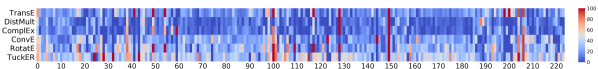
Figure 5. Percentage of triples on which each method outperforms others, separately for each FB15k-237 relation

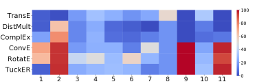
Figure 6. Percentage of triples on which each method outperforms others, for each WN18RR relation

To remove the WN18 reverse relations mentioned in Section 4.2, Dettmers et al. (Dettmers et al., 2018) created WN18RR by keeping just one relation from each pair of reverse relations. The resulting dataset WN18RR has 40,943 entities in 11 relations. However, this dataset still contains symmetric (i.e., self-reciprocal) relations—a special case of reverse relations where a relation is the reverse of itself. Particularly, more than 34% of the training triples in WN18RR belong to the symmetric relation derivationally_related_form which is for terms in different syntactic categories that have the same morphological root. For instance, both triples (question, derivationally_related_form, inquire) and (inquire, derivationally_related_form, question) are in the training set. Among the 11 relations in WN18RR’s training set, 3 are self-reciprocal, which account for 30,933 of the 86,835 training triples. 28,835 out of these 30,933 triples form reverse pairs. For the remaining 2,098 triples, 1,052 form reverse pairs of with 1,052 triples (around 33.57%) of the test set.

As mentioned in Section 4.2, YAGO3-10 has two near-duplicate relations isAffiliatedTo and playsFor and 3 semantically symmetric relations hasNeighbor, isConnectedTo, and isMarriedTo. We removed playsFor. In the training set, for each pair of redundant triples belonging to symmetric relations, we only kept one. Moreover, we removed a triple from the test and validation sets if it belongs to any symmetric relation and its entity pairs are directly linked in the training set. We call the resulting dataset YAGO3-10-DR, of which the statistics can be found in Table 1.

5.2. Experiment Setup

Our experiments were conducted on an Intel-based machine with an Intel Xeon E5-2695 processor running at 2.1GHz, Nvidia Geforce GTX1080Ti GPU, and 256 GB RAM. The experiments used source codes of various methods from several places, including the OpenKE (Han et al., 2018) repository which covers implementations of TransE, TransH, TransR, TransD, RESCAL, DistMult, and ComplEx, as well as the source code releases of ComplEx (which also covers DistMult), ConvE, RotatE, and TuckER. The URLs of these implementations can be found in Table 5.

The different models used in our experiments have different hyperparameters. We used the same hyperparameter settings for FB15k, FB15k-237, WN18, WN18RR, and YAGO3-10 that were used by the developers of the source codes. The details can be found in the codes.

We also experimented with rule-based system AMIE (Galárraga et al., 2013). AMIE rules were generated by applying the AMIE+ (https://bit.ly/2Vq2OIB) code released by the authors of (Galárraga et al., 2015) on the training sets of FB15k, FB15k-237, WN18, WN18RR, and YAGO3-10. The parameters of AMIE+ were set in the same way as in (Meilicke et al., 2018), for all datasets. For any link prediction task (h, r, ?) or (?, r, t), all the rules that have relation r in the rule head are employed. The instantiations of these rules are used to generate the ranked list of results. For example, for test case (Bill Gates, place_of_birth, ?), the following rule will be employed: $(\textsf{\small?a},\textsl{\small places\allowbreak\_lived/location},\textsf{\small?b})\ \Rightarrow(\textsf{\small?a},\textsl{\small place\allowbreak\_of\allowbreak\_birth},\textsf{\small?b})$. Then the instantiations of variable ?b are used to find the list of predictions. Several rules may generate the same answer entity. It is imperative to combine the confidence of those rules in some way in order to score the answer entities. We ranked the answer entities by the maximum confidence of the rules instantiating them and broke ties by the number of applicable rules (Meilicke et al., 2018).

(a) Categorizing the relations on which each method has the best result

(b) Break-down of methods achieving best performance on each type of relations

Figure 7. Models with best FMRR^↑ on FB15k-237

Table 9. FHits@10^↑ by category of relations on FB15k-237

	$1$-to-$1$		$1$-to-$n$		$n$-to-$1$		$n$-to-$m$
Model	Left FH10↑	Right FH10↑	Left FH10↑	Right FH10↑	Left FH10↑	Right FH10↑	Left FH10↑	Right FH10↑
TransE	55.21	55.21	60.40	9.59	11.74	84.60	40.52	56.12
DistMult	47.92	46.35	43.62	3.63	4.34	76.06	36.09	51.48
ComplEx	47.40	46.88	36.66	3.94	5.13	75.82	36.95	52.48
ConvE	27.60	26.56	59.63	11.29	14.38	85.34	41.20	56.73
RotatE	59.38	58.85	67.52	13.61	17.08	87.49	47.38	61.49
TuckER	55.21	52.60	65.58	15.62	21.52	87.84	48.14	61.54
AMIE	43.23	44.27	46.17	13.07	18.20	80.49	42.45	55.19

Table 10. FHits@10^↑ by category of relations on WN18RR

	$1$-to-$1$		$1$-to-$n$		$n$-to-$1$		$n$-to-$m$
Model	Left FH10↑	Right FH10↑	Left FH10↑	Right FH10↑	Left FH10↑	Right FH10↑	Left FH10↑	Right FH10↑
TransE	92.86	92.86	42.32	15.79	14.32	34.90	92.92	93.72
DistMult	97.62	92.86	24.21	6.32	5.78	33.83	95.75	95.75
ComplEx	97.62	97.62	29.47	7.58	5.72	33.02	95.84	95.31
ConvE	97.62	97.62	44.63	16.84	11.57	31.34	95.22	94.96
RotatE	97.62	97.62	53.68	28.84	20.98	43.04	96.11	95.58
TuckER	97.62	97.62	40.21	18.95	15.13	30.26	94.96	91.77
AMIE	97.62	97.62	1.26	1.26	1.41	1.41	92.83	92.83

Table 11. Link prediction results on YAGO3-10

YAGO3-10					YAGO3-10-DR
Model	FH1↑	FMR↓	FH10↑	FMRR↑	FH1↑	FMR↓	FH10↑	FMRR↑
TransE	– 40.7	– 1193.4	– 67.9	– 0.504	– 11.7	– 2355.9	– 32.3	– 0.19
DistMult	– 34.2 42.4	– 1712.8 2685.1	– 64.9 66.0	– 0.448 0.51	– 9.6 13.3	– 7509.3 5553.2	– 28.8 30.7	– 0.161 0.192
ComplEx	– 35.5 44.9	– 3076.4 2911.7	– 64.6 67.8	– 0.455 0.53	– 9.7 14.3	– 8498.1 6077	– 28.8 31.5	– 0.162 0.201
ConvE	45.0 46.2	2792 1598.8	66.0 68.6	0.52 0.542	– 14.7	– 4453.3	– 31.5	– 0.204
RotatE	40.2 40.5	1767 1809.4	67.0 67.4	0.495 0.499	– 15.3	– 3084.2	– 33.2	– 0.214
TuckER	– 40.7	– 2293.8	– 66.1	– 0.496	– 14.8	– 6068.8	– 32	– 0.207
AMIE	55.8	24133	57.96	0.565	–	–	–	–

(a) Categorizing the relations on which each method has the best result

(b) Break-down of methods achieving best performance on each type of relations

Figure 8. Models with best FMRR^↑ on YAGO3-10

Table 12. FHits@10^↑ by category of relations on YAGO31-0

	$1$-to-$1$		$1$-to-$n$		$n$-to-$1$		$n$-to-$m$
Model	Left FH10↑	Right FH10↑	Left FH10↑	Right FH10↑	Left FH10↑	Right FH10↑	Left FH10↑	Right FH10↑
TransE	76.67	80.00	48.31	32.58	3.89	78.34	63.82	80.23
DistMult	83.33	83.33	49.44	29.21	6.09	55.67	60.21	79.77
ComplEx	90.00	83.33	55.06	31.46	5.75	29.10	62.26	80.47
ConvE	83.33	80.00	43.82	39.33	3.21	74.11	65.31	80.98
RotatE	83.33	83.33	55.06	38.20	6.43	77.66	61.66	80.68
TuckER	86.67	90.00	42.70	39.33	5.25	72.59	60.72	79.67
AMIE	73.33	73.33	13.48	11.24	6.26	7.45	67.44	64.24

Table 13. FHits@1^↑ results

Model	FB15k	FB15k-237	WN18	WN18RR
TransE	– 26.9	– 19.1	– 31.1	– 5.1
DistMult	– – 54.1	– 15.5 –	– – 75.2	– 29.1 –
ComplEX	59.9 – 59.5	– 15.9 –	93.6 – 93.7	– 34.0 –
ConvE	67.0 60.7	23.9 23.13	93.5 93.9	39.0 39.2
RotatE	74.6 73.8	24.1 23.9	94.4 94.4	42.8 42.5
TuckER	74.1 72.9	26.6 26.2	94.9 94.6	44.3 42.8
AMIE	– 75.1	– 22.5	– 93.9	– 35.6
Simple Model (generated by us)	71.6	1.1	96.4	34.8

5.3. Results

Tables 5 and 6 display the results of link prediction on FB15k vs. FB15k-237 and WN18 vs. WN18RR for all compared methods, using both raw and filtered metrics explained in Section 3.2. For each method, the table shows the original publication where it comes from. The values in black color are the results listed in the original publication, while a hyphen under a measure indicates that the original publication did not list the corresponding value. The values in other colors are obtained through our experiments using various source codes, as listed in the tables.

Below we summarize and explain the results in Table 5 and Table 6. (1) The overall observation is that the performance of all methods worsens considerably after removal of reverse relations. For instance, the FMRR^↑ of ConvE—one of the best performing methods under many of the metrics—has decreased from 0.698 (on FB15k) to 0.305 (on FB15k-237) and from 0.945 (on WN18) to 0.429 (on WN18RR). Its FMR^↓ also became much worse, from 46.5 (FB15k) to 271.5 (FB15k-237) and from 396.6 (WN18) to 4992.7 (WN18RR). This result verifies that embedding-based methods may only perform well on reverse relations. However, a straightforward approach based on detection of reverse relations can achieve comparable or even better accuracy, as explained in Section 4.2.1.

(2) Many successors of TransE (e.g., DistMult, ComplEx, ConvE, RotatE, and TuckER) were supposed to significantly outperform it. This was indeed verified by our experiment results on FB15k and WN18. However, on FB15k-237, their margin over TransE became much smaller. For example, by FMRR^↑, TransE’s accuracy is 0.288, in comparison with DistMult (0.238), ComplEx (0.249), ConvE (0.305), RotatE (0.337), and TuckER (0.355). We hypothesize that these models improved the results mostly on reverse and duplicate triples and hence, after removing those triples, they do not exhibit clear advantage. This hypothesis can be verified by our finding that most of the test triples on which these models outperformed TransE have reverse or duplicate triples in the training set, as shown in Table 7. The observations regarding WN18RR are similar, although the successors of TransE demonstrated wider edge over TransE. We note that, however, this could be attributed to the large number of reverse triples from symmetric relations that are retained in WN18RR, as explained in Section 5.1.

(3) Tables 5 and 6 show that the performance of AMIE also substantially degenerates in the absence of data redundancy. For example, its FHits@10^↑ has decreased from 88.1% (FB15k) to 47.7% (FB15k-237) and from 94.0% (WN18) to 35.6% (WN18RR).

(4) We further analyzed how the most-accurate models perform. There are 224, 11, and 34 distinct relations in the test sets of FB15k-237, WN18RR, and YAGO3-10, respectively. Table 8 shows, for each metric and each model, the number of distinct test relations on which the model is the most accurate. Furthermore, the heatmap in Figure 5 (Figure 6, resp.) shows, for each of the 224 (11, resp.) relations in FB15k-237 (WN18RR, resp.), the percentage of test triples on which each model has the best performance (i.e., the highest rank) in comparison with other models, using FMRR^↑ as the performance measure. What is particularly insightful about Figure 6 is that TuckER, RotatE, and ConvE clearly dominated other models on relations #1 (derivationally_related_form), #8 (similar_to), and #10 (verb_group). As explained in Section 5.1, these are all symmetric relations where reverse triples are retained in WN18RR. This observation corroborates with the analysis in 2) above. It suggests that the state-of-the-art models might be particularly optimized for reverse triples. On the other hand, the simple rule based on data statistics can attain an FHits@1^↑ of 97.85% on these 3 relations.

(5) To better understand the strengths and weaknesses of each model, we further broke down the numbers in the column FMRR^↑of Table 8. The relations are categorized into 4 different classes: $1$-to-$1$, $1$-to-$n$, $n$-to-$1$ and $n$-to-$m$, based on the average number of heads per tail and tails per head. An average number less than 1.5 is marked as “$1$” and “$n$” otherwise (Bordes et al., 2013). Among the 224 distinct relations in the test set of FB15k-237, 5.8% are $1$-to-$1$, 11.6% are $1$-to-$n$, 33.9% are $n$-$1$, and 48.7% are $n$-to-$m$ relations. The numbers of test triples belonging to these 4 types of relations are 192, 1,293, 4,285 and 14,696, respectively. In WN18RR, the 11 distinct relations in the test set are distributed as 2, 4, 3, and 2 in these four classes, and the numbers of test triples are 42, 475, 1,487, and 1,130, respectively. Figure 7(a) shows the break-down of relations on which each method has the best result for FB15k-237. Figure 7(b) shows the break-down of best performing models within each type of relations. Overall, RotatE and TuckER outperformed other models, with RotatE particularly excelling on $1$-to-$1$ and $1$-to-$n$ relations and TuckER on $n$-to-$1$ and $n$-to-$m$ relations. TransE still demonstrated its robust strength on $1$-to-$1$ relations. Our experiment results on WN18RR show some characteristics similar to that of Figure 7. However, since WN18RR has only 11 relations, the distributions are less indicative and robust. Hence, we omit the discussions of such results on WN18RR.

(6) We further computed the FHits@10^↑ for head and tail predictions separately for each relation type of FB15k-237 and WN18RR, as in Tables 9 and 10. The first and second best results are shown with boldface and underline, respectively. All the methods performed better at predicting the “$1$” side of $1$-to-$n$ and $n$-to-$1$ relations on both datasets. On FB15k-237, RotatE and TransE are the first and second best performing models on $1$-to-$1$ relations, respectively. RoataE and TuckER have the highest performance on $1$-to-$n$, $n$-to-$1$, and $n$-to-$m$ relations. Performance of TuckER, RotatE, and AMIE is the best in predicting the side $n$ of $1$-to-$n$ and $n$-to-$1$ relations which are more complicated. On WN18RR, almost all models have very high accuracy on $1$-to-$1$ and $n$-to-$m$ relations. Note that self-reciprocal relations derivationally_related_form, similar_to, and verb_group belong to these categories.

(7) As mentioned in Section 4.2.2, YAGO3-10 is dominated by two relations isAffilatedTo and playsFor which are effectively duplicate relations. The results on this dataset for some the best performing models are shown in Table 11. AMIE achieved better performance than embedding models on FHits@1^↑and FMRR^↑. Similar to (5) and (6), we generated detailed results on this dataset, shown in Figure 8 and Table 12. Figure 8 shows that AMIE outperformed other models on $1$-to-$1$ and $n$-to-$m$ relations while TuckER was on par with AMIE on $1$-to-$1$ relations. RotatE and TuckER outperformed others in $1$-to-$n$ and $n$-to-$1$ relations. Table 12 shows that embedding models have very similar results particularly on $1$-to-$1$ and $n$-to-$m$ relations. We note that the duplicate relations isAffilatedTo and playsFor belong to $n$-to-$m$ and the self-reciprocal relation isMarriedTo belongs to $1$-to-$1$.

(8) The results on YAGO3-10-DR are also shown in Table 11. Same as what we observed on FB15k-237 and WN18RR, the performance of all models dropped significantly after removal of duplicate and reverse triples. Hence, we recommend YAGO3-10-DR for evaluating embedding models instead of YAGO3-10.

(9) Table 13 compares various methods using FHits@1^↑, which is a more demanding measure than FHits@10^↑, since it only considers whether a model ranks a correct answer at the very top. The results show that embedding models and AMIE have comparable performance on FB15k and WN18 as these datasets contain relations that clearly can be predicted by rules. On FB15k-237 and WN18RR, embedding models RotatE and TuckER stand out.

6. Conclusions

In this paper, we did an extensive investigation of data redundancy in the widely-used benchmark datasets FB15k, WN18, and YAGO3-10 and its impact on the performance of link prediction models. Our experiments show that, in the absence of the straightforward prediction tasks, the performance of these models degenerates significantly. We identified Cartesian product relations in FB15k which also lead to unrealistic evaluation performance. Given the data characteristics, oftentimes a simple rule based on data statistics can challenge the accuracy of complex machine learning models. Moreover, these problems with the data present unrealistic cases of link prediction that are nonexistent in the real world. We also demonstrated the inadequacy of existing evaluation metrics that penalize a method for generating correct predictions not available in the ground-truth dataset. The results of the study render link prediction a task without truly effective automated solution. Hence, we call for re-investigation of possible effective approaches for completing knowledge graphs.

- (1)
- Akrami et al. (2018) Farahnaz Akrami, Lingbing Guo, Wei Hu, and Chengkai Li. 2018. Re-evaluating Embedding-Based Knowledge Graph Completion Methods. In Proceedings of the 27th ACM International Conference on Information and Knowledge Management (CIKM). 1779–1782. https://doi.org/10.1145/3269206.3269266
- Auer et al. (2007) Sören Auer, Christian Bizer, Georgi Kobilarov, Jens Lehmann, Richard Cyganiak, and Zachary Ives. 2007. DBpedia: A nucleus for a web of open data. In Proceedings of the 6th International Semantic Web Conference and 2nd Asian Semantic Web Conference (ISWC + ASWC). 722–735.
- Balažević et al. (2019) Ivana Balažević, Carl Allen, and Timothy M Hospedales. 2019. TuckER: Tensor Factorization for Knowledge Graph Completion. In Proceedings of the 2019 Conference on Empirical Methods in Natural Language Processing and the 9th International Joint Conference on Natural Language Processing (EMNLP + IJCNLP). 5185–5194. https://doi.org/10.18653/v1/D19-1522
- Bollacker et al. (2008) Kurt Bollacker, Colin Evans, Praveen Paritosh, Tim Sturge, and Jamie Taylor. 2008. Freebase: a collaboratively created graph database for structuring human knowledge. In Proceedings of the 2008 ACM international conference on Management of data (SIGMOD). 1247–1250. https://doi.org/10.1145/1376616.1376746
- Bordes et al. (2013) Antoine Bordes, Nicolas Usunier, Alberto Garcia-Durán, Jason Weston, and Oksana Yakhnenko. 2013. Translating embeddings for modeling multi-relational data. In Proceedings of the 26th International Conference on Neural Information Processing Systems (NeurIPS). 2787–2795.
- Cai et al. (2018) Hongyun Cai, Vincent W Zheng, and Kevin Chen-Chuan Chang. 2018. A comprehensive survey of graph embedding: Problems, techniques, and applications. IEEE Transactions on Knowledge and Data Engineering (TKDE) 30, 9 (2018), 1616–1637. https://doi.org/10.1109/TKDE.2018.2807452
- Carlson et al. (2010) Andrew Carlson, Justin Betteridge, Bryan Kisiel, Burr Settles, Estevam R Hruschka Jr, and Tom M Mitchell. 2010. Toward an architecture for never-ending language learning. In Proceedings of the 24th AAAI Conference on Artificial Intelligence (AAAI). 1306–1313.
- Das et al. (2018) Rajarshi Das, Shehzaad Dhuliawala, Manzil Zaheer, Luke Vilnis, Ishan Durugkar, Akshay Krishnamurthy, Alex Smola, and Andrew McCallum. 2018. Go for a Walk and Arrive at the Answer: Reasoning Over Paths in Knowledge Bases using Reinforcement Learning. In Proceedings of the 6th International Conference on Learning Representations (ICLR).
- Dettmers et al. (2018) Tim Dettmers, Minervini Pasquale, Stenetorp Pontus, and Sebastian Riedel. 2018. Convolutional 2D Knowledge Graph Embeddings. In Proceedings of the 32nd AAAI Conference on Artificial Intelligence (AAAI). 1811–1818.
- Eder (2012) Jeffrey Scott Eder. 2012. Knowledge graph based search system. US Patent App. 13/404,109.
- Färber (2017) Michael Färber. 2017. Semantic Search for Novel Information. IOS Press, Amsterdam, The Netherlands, The Netherlands.
- Galárraga et al. (2015) Luis Galárraga, Christina Teflioudi, Katja Hose, and Fabian M. Suchanek. 2015. Fast Rule Mining in Ontological Knowledge Bases with AMIE. The VLDB Journal 24, 6 (Dec. 2015), 707–730. https://doi.org/10.1007/s00778-015-0394-1
- Galárraga et al. (2013) Luis Antonio Galárraga, Christina Teflioudi, Katja Hose, and Fabian Suchanek. 2013. AMIE: association rule mining under incomplete evidence in ontological knowledge bases. In Proceedings of the 22nd international conference on World Wide Web (WWW). 413–422. https://doi.org/10.1145/2488388.2488425
- Han et al. (2018) Xu Han, Shulin Cao, Xin Lv, Yankai Lin, Zhiyuan Liu, Maosong Sun, and Juanzi Li. 2018. OpenKE: An Open Toolkit for Knowledge Embedding. In Proceedings of the 2018 Conference on Empirical Methods in Natural Language Processing: System Demonstrations (EMNLP). 139–144. https://doi.org/10.18653/v1/D18-2024
- Ji et al. (2015) Guoliang Ji, Shizhu He, Liheng Xu, Kang Liu, and Jun Zhao. 2015. Knowledge Graph Embedding via Dynamic Mapping Matrix. In Proceedings of the 53rd Annual Meeting of the Association for Computational Linguistics and the 7th International Joint Conference on Natural Language Processing (ACL + IJCNLP). 687–696. https://doi.org/10.3115/v1/P15-1067
- Lao and Cohen (2010) Ni Lao and William W Cohen. 2010. Relational retrieval using a combination of path-constrained random walks. Machine learning 81, 1 (2010), 53–67. https://doi.org/10.1007/s10994-010-5205-8
- Lin et al. (2018) Xi Victoria Lin, Richard Socher, and Caiming Xiong. 2018. Multi-hop knowledge graph reasoning with reward shaping. In Proceedings of the 2018 Conference on Empirical Methods in Natural Language Processing (EMNLP) (2018), 3243–3253.
- Lin et al. (2015a) Yankai Lin, Zhiyuan Liu, Huanbo Luan, Maosong Sun, Siwei Rao, and Song Liu. 2015a. Modeling Relation Paths for Representation Learning of Knowledge Bases. In Proceedings of the 2015 Conference on Empirical Methods in Natural Language Processing (EMNLP). 705–714. https://doi.org/10.18653/v1/D15-1082
- Lin et al. (2015b) Yankai Lin, Zhiyuan Liu, Maosong Sun, Yang Liu, and Xuan Zhu. 2015b. Learning Entity and Relation Embeddings for Knowledge Graph Completion.. In Proceedings of the 29th AAAI Conference on Artificial Intelligence (AAAI). 2181–2187.
- Mahdisoltani et al. (2015) Farzaneh Mahdisoltani, Joanna Biega, and Fabian M Suchanek. 2015. Yago3: A knowledge base from multilingual wikipedias. In Conference on Innovative Data Systems Research (CIDR).
- Meilicke et al. (2018) Christian Meilicke, Manuel Fink, Yanjie Wang, Daniel Ruffinelli, Rainer Gemulla, and Heiner Stuckenschmidt. 2018. Fine-grained evaluation of rule-and embedding-based systems for knowledge graph completion. In International Semantic Web Conference (ISWC). https://doi.org/10.1007/978-3-030-00671-6_1
- Miller (1995) George A. Miller. 1995. WordNet: A Lexical Database for English. Commun. ACM 38, 11 (Nov. 1995), 39–41.
- Nickel et al. (2016) Maximilian Nickel, Kevin Murphy, Volker Tresp, and Evgeniy Gabrilovich. 2016. A review of relational machine learning for knowledge graphs. Proc. IEEE 104, 1 (2016), 11–33. https://doi.org/10.1109/JPROC.2015.2483592
- Nickel et al. (2011) Maximilian Nickel, Volker Tresp, and Hans-Peter Kriegel. 2011. A Three-Way Model for Collective Learning on Multi-Relational Data. In Proceedings of the 28th International Conference on Machine Learning (ICML). 809–816.
- Pellissier Tanon et al. (2016) Thomas Pellissier Tanon, Denny Vrandečić, Sebastian Schaffert, Thomas Steiner, and Lydia Pintscher. 2016. From Freebase to Wikidata: The Great Migration. In Proceedings of the 25th International Conference on World Wide Web (WWW). 1419–1428.
- Rotmensch et al. (2017) Maya Rotmensch, Yoni Halpern, Abdulhakim Tlimat, Steven Horng, and David Alexander Sontag. 2017. Learning a Health Knowledge Graph from Electronic Medical Records. Scientific Reports 7 (12 2017). https://doi.org/10.1038/s41598-017-05778-z
- Shi and Weninger (2017) Baoxu Shi and Tim Weninger. 2017. ProjE: Embedding projection for knowledge graph completion. In Proceedings of the 31st AAAI Conference on Artificial Intelligence (AAAI). 1236–1242.
- Socher et al. (2013) Richard Socher, Danqi Chen, Christopher D Manning, and Andrew Ng. 2013. Reasoning with neural tensor networks for knowledge base completion. In Proceedings of the 26th International Conference on Neural Information Processing Systems (NeurIPS). 926–934.
- Suchanek et al. (2008) Fabian M Suchanek, Gjergji Kasneci, and Gerhard Weikum. 2008. Yago: A large ontology from wikipedia and wordnet. Web Semantics 6, 3 (2008), 203–217. https://doi.org/10.1016/j.websem.2008.06.001
- Sun et al. (2019) Zhiqing Sun, Zhi-Hong Deng, Jian-Yun Nie, and Jian Tang. 2019. RotatE: Knowledge Graph Embedding by Relational Rotation in Complex Space. In Proceedings of the International Conference on Learning Representations (ICLR). 926–934.
- Toutanova and Chen (2015) Kristina Toutanova and Danqi Chen. 2015. Observed versus latent features for knowledge base and text inference. In Proceedings of the 3rd Workshop on Continuous Vector Space Models and their Compositionality. 57–66. https://doi.org/10.18653/v1/W15-4007
- Trouillon et al. (2016) Théo Trouillon, Johannes Welbl, Sebastian Riedel, Éric Gaussier, and Guillaume Bouchard. 2016. Complex embeddings for simple link prediction. In Proceedings of the 33rd International Conference on Machine Learning (ICML). 2071–2080.
- Tucker et al. (1964) Ledyard R Tucker et al. 1964. The extension of factor analysis to three-dimensional matrices. Contributions to mathematical psychology 110119 (1964).
- Vrandečić and Krötzsch (2014) Denny Vrandečić and Markus Krötzsch. 2014. Wikidata: a free collaborative knowledgebase. Commun. ACM 57, 10 (2014), 78–85.
- Wang et al. (2019) Yanjie Wang, Daniel Ruffinelli, Rainer Gemulla, Samuel Broscheit, and Christian Meilicke. 2019. On Evaluating Embedding Models for Knowledge Base Completion. In Proceedings of the 4th Workshop on Representation Learning for NLP (RepL4NLP-2019). 104–112. https://doi.org/10.18653/v1/W19-4313
- Wang et al. (2014) Zhen Wang, Jianwen Zhang, Jianlin Feng, and Zheng Chen. 2014. Knowledge Graph Embedding by Translating on Hyperplanes. In Proceedings of the 28th AAAI Conference on Artificial Intelligence (AAAI). 1112–1119.
- Weston et al. (2013) Jason Weston, Antoine Bordes, Oksana Yakhnenko, and Nicolas Usunier. 2013. Connecting Language and Knowledge Bases with Embedding Models for Relation Extraction. In Proceedings of the 2013 Conference on Empirical Methods in Natural Language Processing (EMNLP). 1366–1371.
- Xu et al. (2016) Kun Xu, Siva Reddy, Yansong Feng, Songfang Huang, and Dongyan Zhao. 2016. Question Answering on Freebase via Relation Extraction and Textual Evidence. In In Proceedings of the 54th Annual Meeting of the Association for Computational Linguistics (ACL). 2326–2336. https://doi.org/10.18653/v1/P16-1220
- Yang et al. (2015) Bishan Yang, Wen-tau Yih, Xiaodong He, Jianfeng Gao, and Li Deng. 2015. Embedding entities and relations for learning and inference in knowledge bases. In Proceedings of the International Conference on Learning Representations (ICLR).
- Yao and Van Durme (2014) Xuchen Yao and Benjamin Van Durme. 2014. Information extraction over structured data: Question answering with freebase. In Proceedings of the 52nd Annual Meeting of the Association for Computational Linguistics (ACL), Vol. 1. 956–966.
- Yih et al. (2015) Wen-tau Yih, Ming-Wei Chang, Xiaodong He, and Jianfeng Gao. 2015. Semantic Parsing via Staged Query Graph Generation: Question Answering with Knowledge Base. In Proceedings of the 53rd Annual Meeting of the Association for Computational Linguistics and the 7th International Joint Conference on Natural Language Processing (ACL + IJCNLP). 1321–1331. https://doi.org/10.3115/v1/P15-1128