Biexciton State Energies from Many-Body Perturbation Theory Based on Density Functional Theory Simulation

Abstract

We develop a method for computing self-energy of a biexciton state in a semiconductor nanostructure using many-body perturbation theory (MBPT) based on the density functional theory (DFT) simulation. We compute energies of low-energy biexciton states composed of singlet excitons in the chiral single-wall carbon nanotubes (SWCNT), such as (6,2), (6,5) and (10,5). In all cases we find a small decrease in the biexciton gap: -0.045 $eV$ in (6,2), which is 4.59% of the non-interacting biexciton gap; -0.041 $eV$ in (6,5), which is 4.47% of the non-interacting gap and -0.036 $eV$ in (10,5), which is 4.31%.

I Introduction

Efficient photon-to-electron energy conversion is an important property of a nanomaterial, which has been receiving a lot of attention. One mechanism of increasing the conversion efficiency is called multiple-exciton generation (MEG), where absorption of a high-energy photon results in the generation of multiple charge carriers. Fig. 1 illustrates the MEG process: absorption of a high-energy photon creates an electron-hole pair (exciton) with the energy exceeding twice the bandgap. In MEG, this excess photon energy is diverted into generation of additional charge carriers instead of being lost to generating atomic vibrations.

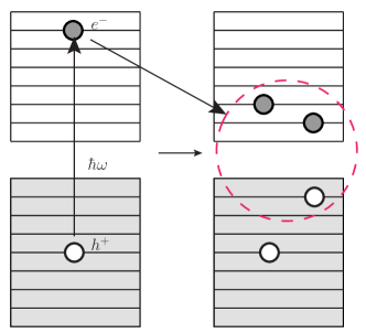
Figure 1: Schematic illustration of the MEG process. Absorption of a photon with energy $\hbar\omega\geq 2E_{gap}$ creates and exciton which can decay into a biexciton. Pictured here, a hot electron loses some of its energy to the creation of another electron-hole pair.

It has been shown that biexciton bound states play an important role in the excited-state properties of SWCNTs and that exciton-exciton binding energies are strongly dependent on the nanotube chirality Matsunaga et al. (2011); Santos et al. (2011). Experimental work aimed at addressing specifically the importance of exciton-exciton interactions in chiral SWCNTs has been performed by Colombier et al., where biexciton binding energy of 106 meV in (9,7) SWCNT has been reported Colombier et al. (2012). Previous theoretical work on exciton and biexciton binding energies in carbon nanotubes has been reported by Kammerlander et al. where the quantum Monte Carlo method has been combined with the tight-binding approximation and binding energies of $\approx 120-150$ meV were reported Kammerlander et al. (2007). Theoretical efforts based on MBPT for calculating exciton-to-biexciton rates in MEG calculations in carbon nanotubes have been reported by Rabani et al., although in their work, the final biexciton state is treated as a pair of two non-interacting excitons Rabani and Baer (2010). Additionally, there has been extensive theoretical work based on perturbation theory aimed at predicting carrier multiplication (CM) rates in semiconductor nanostructures Vörös et al. (2013); Marri et al. (2015, 2014), but exciton-exciton interactions in the final biexciton state are not included. Explicit, first-principles treatment of exciton-exciton interactions in semiconductor nanostructures is reported by Piryatinski et al. Piryatinski et al. (2007), where first-order perturbation theory is applied to biexciton states in type II core/shell nanocrystals, where spatial separation of opposite charges and enhanced confinement of like-charges leads to large ($\sim$ 100 meV) positive shifts to the bi-exciton energies. However, the methodology developed in Piryatinski et al. (2007) is not applicable to biexciton states where exciton separation distance is comparable to electron-hole separation distance, as can be expected in CNTs.

Recently, Kryjevski et al. have developed several methods for a comprehensive description of MEG in a nanosctructure using DFT-based MBPT, including exciton effects Kryjevski and Kilin (2014, 2016); Kryjevski et al. (2016); Kryjevski et al. (2017a, b); Kryjevski et al. (2018). First, one uses DFT-based MBPT technique to compute exciton-to-biexciton decay and recombination rates, i.e., the rates of the inverse and direct Auger processes, respectively Kryjevski and Kilin (2014, 2016). Next, one utilizes DFT software to compute phonon frequencies and normal modes, which are then used to compute one- and two-phonon exciton emission rates Kryjevski et al. (2017b). Finally, all these rates are incorporated into the Boltzmann transport equation (BE) which provides comprehensive nonperturbative description of time evolution of the excited state including “competition” between different relaxation channels, such as MEG, phonon-mediated relaxation, etc. Kryjevski et al. (2017b). In particular, one can compute number of excitons generated from a single high-energy photon, which is the internal quantum efficiency (QE). This method has been successfully applied to several chiral SWCNTs and efficient low-energy MEG was predicted, in a good agreement with the available experimental data Wang et al. (2010); Gabor et al. (2009). Further, when augmented with the exciton transfer terms this BE technique has been applied to the doped SWCNT-$Si$ nanocrystal system and formation of a long-lived charge transfer state was predicted Kryjevski et al. (2018). Additionally, in Kryjevski et al. (2017a) MEG rates method for the singlet fission (SF) process, where a singlet exciton decays into two spin-one (triplet) excitons in the overall singlet state, has been developed and applied to SWCNTs.

In all the MEG work so far the final biexciton state has been approximated as a non-interacting exciton pair. However, knowledge of the low-energy biexciton energy levels is essential for the accurate prediction of the MEG threshold. So, here we investigate this issue by developing a DFT-based MBPT method for biexciton state energies by including residual electrostatic (dipole-dipole) interactions between the excitons in the biexciton state. The technique is then applied to chiral SWCNTs (6,2), (6,5) and (10,5). Here, only biexciton states composed of two singlet excitons are included.

The paper is organized as follows. Section II contains description of the methods and approximations employed in this work. Section IV contains description of the atomistic models studied in this work and of DFT simulation details. Section V contains discussion of the results obtained. Conclusions and Outlook are presented in Section VI.

II Theoretical Methods and Approximations

II.1 Microscopic Hamiltonian

For completeness, let us review basics of the DFT-based MBPT approach that includes electron-exciton terms Kryjevski et al. (2017a).

The electron field operator $\psi_{\sigma}(\textbf{x})$ is related to the annihilation operator of the $i^{th}$ Kohn-Sham (KS) state $a_{i\alpha}$ via

$$\psi_{\sigma}(\textbf{x})=\sum_{i,\sigma}\phi_{i\sigma}(\textbf{x})a_{i\sigma}$$ (1)

where $\phi_{i\sigma}(\textbf{x})$ is the $i^{th}$ KS orbital with spin $\sigma$ and $a_{i\sigma},a_{i\sigma}^{\dagger}$ obey fermion anti-commutation relations $\{a_{i\sigma},a_{j\nu}^{\dagger}\}=\delta_{ij}\delta_{\sigma\nu},\{a_{i\sigma},a_{j\nu}\}=0$ Fetter and Walecka (1971); Mahan (2000). In the spin nonpolarized case we consider here, $\phi_{i\uparrow}(\textbf{x})=\phi_{i\downarrow}(\textbf{x})\equiv\phi_{i}(\textbf{x}).$ In terms of $a_{i\sigma},a_{i\sigma}^{\dagger}$, the electron Hamiltonian is

$${H}=\sum_{i\sigma}\varepsilon_{i}a_{i\sigma}^{\dagger}a_{i\sigma}+H_{C}-H_{V}+H_{e-exciton}$$ (2)

where $\varepsilon_{i\uparrow}=\varepsilon_{i\downarrow}\equiv\varepsilon_{i}$ is the energy of the $i^{\text{th}}$ KS orbital. In a periodic structure KS energies and orbitals are labeled by the band number and lattice wavevector but here, as explained in Sec. IV, the state label is just an integer. The $H_{C}$ term is the microscopic Coulomb interaction operator

$$H_{C}=\frac{1}{2}\sum_{ijkl\sigma,\nu}V_{ijkl}a^{\dagger}_{i\sigma}a^{\dagger}_{j\nu}a_{l\nu}a_{k\sigma},$$ (3)

$$V_{ijkl}=\int d\textbf{x}d\textbf{y}\phi_{i}^{*}(\textbf{x})\phi_{j}^{*}(\textbf{y})\frac{e^{2}}{|\textbf{x}-\textbf{y}|}\phi_{l}(\textbf{y})\phi_{k}(\textbf{x}),$$ (4)

where KS indices $i,j,k,l,...$ can refer to both occupied and unoccupied states within the included range. The $H_{V}$ term prevents double-counting of electron interactions

$$H_{V}=\sum_{ij,\sigma}a^{\dagger}_{i\sigma}\bigg{(}\int d\textbf{x}d\textbf{y}\phi_{i}^{*}(\textbf{x})V_{KS}(\textbf{x},\textbf{y})\phi_{j}(\textbf{y})\bigg{)}a_{j\sigma},$$ (5)

where $V_{KS}(\textbf{x},\textbf{y})$ is the Kohn-Sham potential used in the DFT simulation Onida et al. (2002); Kümmel and Kronik (2008).

The electron-exciton coupling term $H_{e-exciton}$ appearing in Eq. (2) is

$$H_{e-exciton}=\sum_{eh\alpha}\sum_{\sigma}\frac{1}{\sqrt{2}}\bigg{(}[\varepsilon_{e}-\varepsilon_{h}-E^{\alpha}]\Psi_{eh}^{\alpha}a_{h\sigma}a^{\dagger}_{e\sigma}({\rm B}^{\alpha}+{\rm B}^{\alpha\dagger})+h.c.\bigg{)}+\sum_{\alpha}E^{\alpha}{\rm B}^{\alpha\dagger}{\rm B}^{\alpha}$$ (6)

where $e\geq$ LU (the lowest unoccupied KS state) and $h\leq HO$ (the highest occupied KS state), ${\rm B}^{\alpha\dagger}$, $\Psi_{eh}^{\alpha}$ and $E^{\alpha}$ are the singlet exciton creation operator, wave function and energies respectively. Technically, the full electron Hamiltonian is comprised of only the first three terms in Eq. (2), however adding $H_{e-exciton}$ along with the rules to avoid double counting allows for the perturbative treatment of excitonic effects and is a standard approch to describing the coupling between excitons and electrons and holes Beane et al. (2000); Spataru et al. (2004); Perebeinos et al. (2004); Spataru et al. (2005). The $H_{e-exciton}$ term is a result of resummation of Coulomb perturbative corrections resulting from the Coulomb interaction operator $H_{C}$ (Eq. (4)) to the electron-hole state, which is an implementation of a standard method to include bound states into the MBPT framework Berestetskii et al. (1979); Beane et al. (2000); Kryjevski et al. (2017a).

Exciton wave functions, $\Psi_{eh}^{\alpha},$ and energies, $E^{\alpha},$ are solutions to the Bethe-Salpeter equation (BSE), which is (see, e.g., Benedict et al. (2003a))

$$[\varepsilon_{e}-\varepsilon_{h}-E^{\alpha}]\Psi_{eh}^{\alpha}+\sum_{e^{\prime}h^{\prime}}(K_{C}+K_{D})(e,h;e^{\prime},h^{\prime})\Psi_{e^{\prime}h^{\prime}}^{\alpha}=0,$$ (7)

where

$$K_{C}=\frac{8\pi e^{2}}{V}\sum_{\textbf{k}\neq 0}\frac{\rho_{eh}(\textbf{k})\rho_{e^{\prime}h^{\prime}}^{*}(\textbf{k})}{k^{2}},$$ (8)

$$K_{D}=-\frac{4\pi e^{2}}{V}\sum_{\textbf{k}\neq 0}\frac{\rho_{ee^{\prime}}(\textbf{k})\rho_{hh^{\prime}}^{*}(\textbf{k})}{|\textbf{k}|^{2}-\Pi(0,-\textbf{k},\textbf{k})},$$ (9)

where

$$\rho_{ij}(\textbf{k})=\sum_{\textbf{p}}\phi_{j}^{*}(\textbf{p}-\textbf{k})\phi_{i}(\textbf{p})$$ (10)

Medium screening is taken into account via the polarization function (Eq. (11)) which appears only in the direct term (Eq. (9)) of BSE. In the random-phase approximation (RPA)

$$\Pi(\omega,\textbf{k},\textbf{p})=\frac{8\pi e^{2}}{\hbar V}\sum_{ij}\rho_{ij}(\textbf{k})\rho_{ji}(\textbf{p})\bigg{(}\frac{\theta_{-j}\theta_{i}}{\omega-\omega_{ij}+i\delta}-\frac{\theta_{j}\theta_{-i}}{\omega-\omega_{ij}-i\delta}\bigg{)},\;\;\;\omega_{ij}=\frac{\varepsilon_{i}-\varepsilon_{j}}{\hbar}$$ (11)

where $V$ is the simulation cell volume, $\delta$ is the width parameter, which will be set to $0.025~{}eV$ corresponding to the room temperature scale.

Here, we use static approximation, taking $\Pi(\omega=0,\textbf{k},\textbf{p}).$ This is a widely-used approach for semiconductor nanostructures (e.g., Öğüt et al. (2003); Benedict et al. (2003b); Wilson et al. (2009)), which is justified by the cancellations that appear when the electron-hole screening and the single-particle Green’s functions are both treated dynamically Bechstedt et al. (1997). Next, the main simplifying approximation employed in this work is to retain only the diagonal elements of the polarization matrix, i.e., $\Pi(0,\textbf{k},\textbf{p})\simeq\Pi(0,\textbf{k},-\textbf{k})\delta_{\textbf{k},-\textbf{p}}$, or $\Pi(0,\textbf{x},\textbf{x}^{\prime})\simeq\Pi(0,\textbf{x}-\textbf{x}^{\prime})$ in position space, i.e., the system is approximated as a uniform medium. This is a valid approximation for quasi-one-dimensional systems, such as CNTs, where one can expect $\Pi(\textbf{x},\textbf{x}^{\prime})\simeq\Pi(z-z^{\prime})$, with $z,z^{\prime}$ being the axial positions. This diagonal polarization matrix approximation, which is a an improvement on previous studies on CNTs in which screening has been approximated by a dielectric constant Perebeinos and Avouris (2006), has been employed for the time being, as it significantly reduces computational costs. Calculations including full treatment of the polarization matrix, although unlikely to change qualitative conclusions, are left for future work. Also, in the DFT simulations one uses hybrid Heyd-Scuseria-Ernzerhof (HSE06) exchange-correlation functional Heyd et al. (2003) which is to substitute for the $G_{0}W_{0}$ calculation of single-particle energies - the second step in the standard three-step process in the electronic structure calculation Rohlfing and Louie (2000); Hybertsen and Louie (1986). The HSE06 functional, which is significantly less computationally expensive than $G_{0}W_{0}$, has been shown to produce somewhat reasonable results for bandgaps in semiconducting nanostructures Kümmel and Kronik (2008); Muscat et al. (2001); Jain et al. (2011). So, single-particle energies and orbitals are approximated by the KS $\varepsilon_{i}$ and $\phi_{i}({\bf x})$ from the HSE06 DFT output. Therefore, in our approximation using HSE06 replaces “dressing” fermion lines in the Feynman diagrams, including subtraction of the compensating term (5).

For SWCNTs, the set of approximations stated above have been checked and shown to be reasonable by reproducing experimental results for the low-energy absorption peaks in (6,2), (6,5) and (10,5) SWCNTs within 5-13% error Kryjevski et al. (2017b).

III Expressions for the Biexciton Self-Energy

In order to account for the exciton-exciton interactions one computes self-energy of the biexciton state $\hbar\Sigma_{\alpha\beta}(E)$. Then the biexciton energy is approximated as

$$E_{\alpha\beta}=E^{\alpha}+{E}^{\beta}+\hbar\Sigma_{\alpha\beta}(E=E^{\alpha}+E^{\beta})$$ (12)

where $E^{\alpha}$ and $E^{\beta}$ are the energies of the two excitons in the biexciton state. $E^{\alpha}$ and $E^{\beta}$ are obtained by solving the Bethe-Salpeter equation (Eq. (7)). $\hbar\Sigma_{\alpha\beta}(E=E^{\alpha}+E^{\beta})$ is the biexciton self-energy evaluated on the total energy of a state composed of two non-interacting excitons $|{\alpha}\rangle$ and $|{\beta}\rangle$.

To the leading order in the Coulomb interaction the relevant Feynman diagrams are shown in Fig. 2. One only retains corrections to the bare biexciton state where a particle or a hole from the exciton $|{\alpha}\rangle$ interacts with a particle or a hole from the other exciton $|{\beta}\rangle$; the interactions between particles and holes within the same exction are already included by the BSE. Note that including contributions with all possible arrow directions in each fermion loop is needed to include all the interactions between electrons and holes within the biexciton state.

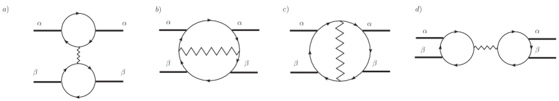
Figure 2: Leading order Feynman diagrams representing contributions to the biexciton self-energy. Thin (fermion) lines are Kohn-Sham particle/hole propagators, thick lines - excitons (see Fig. 3), zigzag lines - the screened Coulomb interaction. Not shown for brevity are similar diagrams where arrow directions in one of the fermion loops are reversed, and diagrams where all arrows are reversed.

Note that for each diagram in Fig. 2 there is an additional contribution upon exchange of the $\alpha$ and $\beta$ excitons on the right-hand-side of the fermion loop. These contributions are currently a subject of future work. The expressions resulting from each diagram in Fig. 2 are similar in general form, so for brevity, only one of them will be quoted here and the rest will be presented in the appendix. For instance, the diagram from Fig. 2 - a) results in the following expression

$$\hbar\Sigma_{\alpha\beta}(E=E^{\alpha}+E^{\beta})=\frac{4}{5}\sum_{ijklmn}\frac{\Theta_{i}\Theta_{n}\Theta_{l}\Theta_{-k}\Theta_{-j}\Theta_{-m}}{(E^{\alpha}-\epsilon_{nk}-i\delta)(E^{\beta}-\epsilon_{lm}+i\delta)(\epsilon_{kj}-i\delta)(\epsilon_{li}+i\delta)}\times$$

$$\times(\Psi_{im}^{\beta})^{*}(E^{\beta}-\epsilon_{im})(\Psi_{nk}^{\alpha})^{*}(E^{\alpha}-\epsilon_{nk})\Psi_{lm}^{\beta}(E^{\beta}-\epsilon_{lm})\Psi_{nj}^{\alpha}(E^{\alpha}-\epsilon_{nj})\times W_{ijkl}$$ (13)

where $\Psi_{ij}^{\alpha}$ and $E^{\alpha}$ are the exciton wave function and exciton energies respectively obtained by solving the Bethe-Salpeter equation (Eq. (7)). $\epsilon_{ij}=\epsilon_{i}-\epsilon_{j}$; $W_{ijkl}$ are the RPA-screened Coulomb matrix elements

$$W_{ijkl}=\frac{4\pi e^{2}}{V}\sum_{\textbf{k}\neq 0}\frac{\rho_{il}^{*}(\textbf{k})\rho_{jk}(\textbf{k})}{|\textbf{k}|^{2}-\Pi(0,-\textbf{k},\textbf{k})}$$ (14)

where $\Pi(0,-\textbf{k},\textbf{k})$ is defined in Eq. (11). The theta-functions determine whether the KS indices $i,j,k,l$ are particles or holes

$$\Theta_{i}=\sum_{i>\text{HO}}~{}~{},~{}~{}\Theta_{-i}=\sum_{i\leq\text{HO}}.$$ (15)

In this work we use

$$\frac{1}{x\pm i\delta}=\frac{x}{x^{2}+\delta^{2}}\mp i\frac{\delta}{x^{2}+\delta^{2}},$$ (16)

i.e., both the principal value and delta function parts of $1/(x\pm i\delta)$ factors are included.

The other three diagrams - 2-$b),~{}c),~{}d)$ - produce similar expressions not shown for the sake of brevity.

Next, the possibility of including higher order perturbative corrections was explored. Naively including terms of second (or higher) order in the Coulomb interaction, i.e., decorating diagrams in Fig. 2 with additional zigzag lines, would lead to prohibitively expensive calculations, even for a small system. However, certain classes of perturbative contributions can be summed to all orders, such as the Coulomb interactions between electron and hole resulting in formation of an exciton bound state (see Fig. 3). Eq. 6 describes the resulting exciton-electron coupling term.

Figure 3: Summing perturbative contributions from Coulomb interactions (zigzag lines) between electron and hole (thin lines) is equivalent to including intermediate exciton bound state (thick line).

This summation of Coulomb corrections to all orders can be applied to modify the diagrams shown in Fig. 2. In Fig. 4 it is illustrated how an intermediate exciton state $\gamma$ appears from decorating the electron-hole lines in Fig. 2 with zigzag lines in all possible ways. Here, we work to the leading order in the electron-exciton coupling - Eq. 6 - and, so, only decorate one pair of the electron-hole lines.

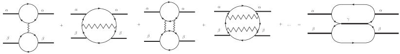
Figure 4: Summing perturbative contributions from Coulomb interactions (zigzag lines) between electron and hole (thin lines) from different excitons - $\alpha$ and $\beta$ - results in appearance of the intermediate exciton $\gamma$.

The two distinct diagrams resulting from modifying Fig. 2 are shown in Fig. 5.

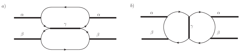
Figure 5: a) - diagram resulting from modification of diagrams 2-a) and b). b) - diagram resulting from modification of diagrams 2-c) and d).

The contributions to the biexciton self-energy from the diagrams in Fig. 5 are

$$\hbar\Sigma_{\alpha\beta}^{+}=\hbar\Sigma_{\alpha\beta}^{\textrm{a}}+\hbar\Sigma_{\alpha\beta}^{\textrm{b}}$$ (17)

$$\hbar\Sigma_{\alpha\beta}^{\textrm{a}}(E=E^{\alpha}+E^{\beta})=\frac{8}{45}\sum_{ijklmn\gamma}\frac{\Theta_{j}\Theta_{k}\Theta_{n}\Theta_{-i}\Theta_{-l}\Theta_{-m}}{(E^{\alpha}-\epsilon_{ki}+i\delta)(E^{\beta}-\epsilon_{nm}-i\delta)(E^{\gamma}-\epsilon_{km}+i\delta)(E^{\gamma}-\epsilon_{jl}+i\delta)(\epsilon_{jk}+i\delta)}\times$$ (18)

$$\times(\Psi_{ji}^{\alpha})^{*}(E^{\alpha}-\epsilon_{ji})\Psi_{ki}^{\alpha}(E^{\alpha}-\epsilon_{ki})\Psi_{nl}^{\beta}(E^{\beta}-\epsilon_{nl})(\Psi_{nm}^{\beta})^{*}(E^{\beta}-\epsilon_{nm})\Psi_{jl}^{\gamma}(E^{\gamma}-\epsilon_{jl})(\Psi_{km}^{\gamma})^{*}(E^{\gamma}-\epsilon_{km})$$

$$\hbar\Sigma_{\alpha\beta}^{\textrm{b}}(E^{\alpha}+E^{\beta})=\frac{8}{45}\sum_{ijklmn\gamma}\frac{\Theta_{j}\Theta_{k}\Theta_{n}\Theta_{-i}\Theta_{-l}\Theta_{-m}}{(E^{\alpha}-\epsilon_{kl}+i\delta)(E^{\beta}-\epsilon_{km}-i\delta)(E^{\gamma}-\epsilon_{jl}+i\delta)(E^{\gamma}-\epsilon_{nm}+i\delta)(\epsilon_{jn}+i\delta)}\times$$ (19)

$$\times(\Psi_{ji}^{\alpha})^{*}(E^{\alpha}-\epsilon_{ji})\Psi_{kl}^{\alpha}(E^{\alpha}-\epsilon_{kl})\Psi_{ni}^{\beta}(E^{\beta}-\epsilon_{ni})(\Psi_{km}^{\beta})^{*}(E^{\beta}-\epsilon_{km})\Psi_{jl}^{\gamma}(E^{\gamma}-\epsilon_{jl})(\Psi_{nm}^{\gamma})^{*}(E^{\gamma}-\epsilon_{nm})$$

where the additional summation label $\gamma$ is over the intermediate exciton state. Note that here the screened Coulomb interaction only appears implicitly through the exciton wavefunctions and energies.

Additionally, there are self-energy contributions from the repulsive electron-electron and hole-hole interactions. These come from, e.g., diagrams in Fig. 2 a) and d) but with arrows in one of the fermion loops reversed. These corrections are treated to the leading order in the Coulomb interaction. There are eight distinct expressions contributing to the biexciton self-energy due to the inter-exciton electron-electron or hole-hole interactions, two from each of the 4 diagrams in Fig. 2 with the appropriate fermion arrow flips. The expressions are

$$\hbar\Sigma_{\alpha\beta}^{-}=\hbar\Sigma_{\alpha\beta}^{\textrm{ee},a}+\hbar\Sigma_{\alpha\beta}^{\textrm{hh},a}+\hbar\Sigma_{\alpha\beta}^{\textrm{ee},b}+\hbar\Sigma_{\alpha\beta}^{\textrm{hh},b}+\hbar\Sigma_{\alpha\beta}^{\textrm{ee},c}+\hbar\Sigma_{\alpha\beta}^{\textrm{hh},c}+\hbar\Sigma_{\alpha\beta}^{\textrm{ee},d}+\hbar\Sigma_{\alpha\beta}^{\textrm{hh},d}$$ (20)

$$\hbar\Sigma_{\alpha\beta}^{\textrm{ee},a}(E^{\alpha}+E^{\beta})=-\frac{4}{5}\sum_{ijklmn}\frac{\Theta_{i}\Theta_{l}\Theta_{k}\Theta_{j}\Theta_{-m}\Theta_{-n}}{(E^{\alpha}+\epsilon_{kn}-i\delta)(E^{\beta}-\epsilon_{lm}+i\delta)(\epsilon_{kj}-i\delta)(\epsilon_{li}+i\delta)}\times$$

$$\times(\Psi_{im}^{\beta})^{*}(E^{\beta}-\epsilon_{im})(\Psi_{kn}^{\alpha})^{*}(E^{\alpha}-\epsilon_{kn})\Psi_{lm}^{\beta}(E^{\beta}-\epsilon_{lm})\Psi_{jn}^{\alpha}(E^{\alpha}-\epsilon_{jn})\times W_{ijkl}$$ (21)

$$\hbar\Sigma_{\alpha\beta}^{\textrm{hh},a}(E^{\alpha}+E^{\beta})=-\frac{4}{5}\sum_{ijklmn}\frac{\Theta_{-i}\Theta_{-l}\Theta_{-k}\Theta_{-j}\Theta_{m}\Theta_{n}}{(E^{\alpha}+\epsilon_{nk}-i\delta)(E^{\beta}-\epsilon_{ml}+i\delta)(\epsilon_{kj}-i\delta)(\epsilon_{li}+i\delta)}\times$$

$$\times(\Psi_{mi}^{\beta})^{*}(E^{\beta}-\epsilon_{mi})(\Psi_{nk}^{\alpha})^{*}(E^{\alpha}-\epsilon_{nk})\Psi_{ml}^{\beta}(E^{\beta}-\epsilon_{ml})\Psi_{nj}^{\alpha}(E^{\alpha}-\epsilon_{nj})\times W_{ijkl}$$ (22)

$$\hbar\Sigma_{\alpha\beta}^{\textrm{ee},b}(E^{\alpha}+E^{\beta})=-\frac{4}{5}\sum_{ijklmn}\frac{\Theta_{i}\Theta_{l}\Theta_{k}\Theta_{j}\Theta_{-m}\Theta_{-n}}{(E^{\alpha}+\epsilon_{im}-i\delta)(E^{\beta}-\epsilon_{ln}+i\delta)(\epsilon_{il}-i\delta)(\epsilon_{jk}+i\delta)}\times$$

$$\times(\Psi_{kn}^{\beta})^{*}(E^{\beta}-\epsilon_{kn})(\Psi_{jm}^{\alpha})^{*}(E^{\alpha}-\epsilon_{jm})\Psi_{ln}^{\beta}(E^{\beta}-\epsilon_{ln})\Psi_{im}^{\alpha}(E^{\alpha}-\epsilon_{im})\times W_{ijkl}$$ (23)

$$\hbar\Sigma_{\alpha\beta}^{\textrm{hh},b}(E^{\alpha}+E^{\beta})=-\frac{4}{5}\sum_{ijklmn}\frac{\Theta_{-i}\Theta_{-l}\Theta_{-k}\Theta_{-j}\Theta_{m}\Theta_{n}}{(E^{\alpha}-\epsilon_{mi}-i\delta)(E^{\beta}-\epsilon_{nl}+i\delta)(\epsilon_{il}-i\delta)(\epsilon_{jk}+i\delta)}\times$$

$$\times(\Psi_{nk}^{\beta})^{*}(E^{\beta}-\epsilon_{nk})(\Psi_{mj}^{\alpha})^{*}(E^{\alpha}-\epsilon_{mj})\Psi_{nl}^{\beta}(E^{\beta}-\epsilon_{nl})\Psi_{mi}^{\alpha}(E^{\alpha}-\epsilon_{mi})\times W_{ijkl}$$ (24)

$$\hbar\Sigma_{\alpha\beta}^{\textrm{ee},c}(E^{\alpha}+E^{\beta})=-\frac{4}{5}\sum_{ijklmn}\frac{\Theta_{i}\Theta_{l}\Theta_{k}\Theta_{j}\Theta_{-m}\Theta_{-n}}{(E^{\alpha}+\epsilon_{im}-i\delta)(E^{\beta}-\epsilon_{jm}+i\delta)(\epsilon_{il}-i\delta)(\epsilon_{jk}+i\delta)}\times$$

$$\times(\Psi_{kn}^{\beta})^{*}(E^{\beta}-\epsilon_{kn})(\Psi_{ln}^{\alpha})^{*}(E^{\alpha}-\epsilon_{ln})\Psi_{jm}^{\beta}(E^{\beta}-\epsilon_{jm})\Psi_{im}^{\alpha}(E^{\alpha}-\epsilon_{im})\times W_{ijkl}$$ (25)

$$\hbar\Sigma_{\alpha\beta}^{\textrm{hh},c}(E^{\alpha}+E^{\beta})=-\frac{4}{5}\sum_{ijklmn}\frac{\Theta_{-i}\Theta_{-l}\Theta_{-k}\Theta_{-j}\Theta_{m}\Theta_{n}}{(E^{\alpha}-\epsilon_{mi}-i\delta)(E^{\beta}+\epsilon_{mj}+i\delta)(\epsilon_{il}-i\delta)(\epsilon_{jk}+i\delta)}\times$$

$$\times(\Psi_{nk}^{\beta})^{*}(E^{\beta}-\epsilon_{nk})(\Psi_{nl}^{\alpha})^{*}(E^{\alpha}-\epsilon_{nl})\Psi_{mj}^{\beta}(E^{\beta}-\epsilon_{mj})\Psi_{mi}^{\alpha}(E^{\alpha}-\epsilon_{mi})\times W_{ijkl}$$ (26)

$$\hbar\Sigma_{\alpha\beta}^{\textrm{ee},d}(E^{\alpha}+E^{\beta})=-\frac{4}{5}\sum_{ijklmn}\frac{\Theta_{i}\Theta_{l}\Theta_{k}\Theta_{j}\Theta_{-m}\Theta_{-n}}{(E^{\alpha}-\epsilon_{im}-i\delta)(E^{\beta}+\epsilon_{lm}+i\delta)(\epsilon_{il}+i\delta)(\epsilon_{kj}-i\delta)}\times$$

$$\times(\Psi_{kn}^{\beta})^{*}(E^{\beta}-\epsilon_{kn})(\Psi_{jn}^{\alpha})^{*}(E^{\alpha}-\epsilon_{jn})\Psi_{lm}^{\beta}(E^{\beta}-\epsilon_{lm})\Psi_{im}^{\alpha}(E^{\alpha}-\epsilon_{im})\times W_{ijkl}$$ (27)

$$\hbar\Sigma_{\alpha\beta}^{\textrm{hh},d}(E^{\alpha}+E^{\beta})=-\frac{4}{5}\sum_{ijklmn}\frac{\Theta_{-i}\Theta_{-l}\Theta_{-k}\Theta_{-j}\Theta_{m}\Theta_{n}}{(E^{\alpha}+\epsilon_{mi}-i\delta)(E^{\beta}-\epsilon_{ml}+i\delta)(\epsilon_{il}+i\delta)(\epsilon_{kj}-i\delta)}\times$$

$$\times(\Psi_{nk}^{\beta})^{*}(E^{\beta}-\epsilon_{nk})(\Psi_{nj}^{\alpha})^{*}(E^{\alpha}-\epsilon_{nj})\Psi_{ml}^{\beta}(E^{\beta}-\epsilon_{ml})\Psi_{mi}^{\alpha}(E^{\alpha}-\epsilon_{mi})\times W_{ijkl},$$ (28)

where, for example, $\hbar\Sigma_{\alpha\beta}^{\textrm{ee},a}$ stands for a self-energy contribution from a diagram representing electron-electron interactions obtained by flipping the arrows in one of the fermion loops in Fig. 2-a). Other symbols hold the same meaning as in Eq. (13). Note that here, Coulomb matrix elements $W_{ijkl}$ have either all-electron or all-hole indices. Thus, the complete expression for the biexciton self-energy is

$$\hbar\Sigma_{\alpha\beta}=\hbar\Sigma_{\alpha\beta}^{+}+\hbar\Sigma_{\alpha\beta}^{-}$$ (29)

where $\hbar\Sigma_{\alpha\beta}^{+}$ is defined in (17) and $\hbar\Sigma_{\alpha\beta}^{-}$ is defined in (20).

IV Atomistic Models

Calculations of biexciton self-energies have been performed for chiral SWCNTs (6,5), (6,2) and (10,5), which are shown in Fig. 6. DFT with HSE06 functional, as implemented in VASP (Vienna ab-initio simulation package) Kresse and Joubert (1999), was used to optimize geometries and obtain KS orbitals $\phi_{i\sigma}(\textbf{x})$ and energies $\varepsilon_{i}$. The momentum cutoff is defined as

$$\frac{\hbar^{2}\textbf{k}^{2}}{2m}\leq E_{max},\;\;\;\textbf{k}=2\pi\bigg{(}\frac{n_{x}}{L_{x}},\frac{n_{y}}{L_{y}},\frac{n_{z}}{L_{z}}\bigg{)},\;\;\;n_{x},n_{y},n_{z}=0,\pm 1,\pm 2,\cdots$$ (30)

where $m$ is the electron mass; we used $E_{max}=300~{}eV$. The number of orbitals used in the calculations was determined by the condition $E_{i_{max}}-E_{HO}\simeq E_{LU}-E_{i_{min}}\geq 3.5~{}eV$ where $i_{max}$/$i_{min}$ label the highest/lowest orbital.

Periodic boundary conditions were used in the DFT simulations. In the axial direction the simulation cell length was chosen to accommodate an integer number of unit cells, while in the other two directions the SWCNT surfaces were separated by about 1 $nm$ of vacuum in order to avoid spurious interactions between their periodic images. For (6,2) and (10,5) the simulations have been performed including three unit cells. The rationale for this is that future work will involve SWCNTs with functionalized surfaces. So, including several unit cells will allow to keep the dopant concentration reasonably low. Also, including three unit cells instead of one substitutes for the Brillouin zone sampling. So, here we perform calculations at the $\Gamma$ point only. Previously, it has been shown that the variations in the single particle energies over the Brillouin zone is reasonably small ($\approx 10\%$) when three unit cells have been included in the simulation instead of one Kryjevski et al. (2017b). For the (6,5) SWCNT only one unit cell was included due to high computational cost. However, the absorption spectrum for (6,5) was reproduced with the same accuracy as for the other two CNTs Kryjevski et al. (2017b).

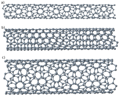
Figure 6: Atomistic models of the three chiral SWCNTs: a) - (6,2), b) - (6,5) and c) - (10,5)

V Results and Discussion

Table 1 shows the results for the three SWCNTs. In all cases the resulting $\Sigma_{\alpha\beta}({E}_{\alpha}+{E}_{\beta})$ come out to be real, with vanishingly small imaginary parts. This is as expected since in our approximation we only include the possibility of the biexciton state decaying into an exciton and an electron-hole pair, which is suppressed due to energy conservation. The biexciton self-energy correction to the biexciton gap was obtained by evaluating Eqs. (13) and (18) for a biexciton state made of two lowest-energy excitons, i.e., $\hbar\Sigma(E=2E_{\rm gap}^{\rm exc}),~{}E_{\rm gap}^{\rm exc}={E}_{1}$. For reference, the quasiparticle gap $E_{\rm gap}=\varepsilon_{LU}-\varepsilon_{HO}$ obtained from the DFT simulation is included. Figure 7 shows plots of the density of states (DOS) for the excitons and biexcitons, including the shift due to exciton-exciton interactions. The DOS was calculated using DOS$=\sum_{i}\delta(E-E_{i})$, where the delta function was approximated by a Gaussian function with a width corresponding to room temperature. For the exciton DOS, $E_{i}$ are the solutions to the Bethe-Salpeter equation - $E_{\alpha}$ (Eq. (7)). For biexciton DOS, $E_{i}=E_{\alpha}+E_{\beta}$ for a pair of non-interacting excitons and $E_{i}=E_{\alpha\beta}$ (Eq. (12)) for the self-energy corrected pair of excitons.

Chirality	$E_{gap}$	$E_{\rm gap}^{\rm exc}$	$\Sigma(2E_{\rm gap}^{\rm exc})$
$(6,2)$	1.33	0.98	-0.045
$(6,5)$	1.22	1.09	-0.041
$(10,5)$	0.91	0.835	-0.036

Table 1: $E_{gap}$ is the HO-LU gap and $E_{\rm gap}^{\rm exc}=\epsilon_{1}$ is the lowest exciton energy obtained from BSE. $\Sigma(2E_{\rm gap}^{\rm exc})$ is the biexciton self-energy for the lowest-energy biexciton. All energies are in $eV$.

Figure 7: Exciton and biexciton DOS for the three nanotubes in units of exciton gap $E_{\rm gap}^{\rm exc}$ . Blue line is the exciton DOS, red line - biexciton DOS without self-energy corrections, green line - biexciton DOS with self-energy corrections.

Results show a small redshift in the biexciton density of states for all the nanostructures under consideration. As a percentage of the non-interacting gap, these shifts are: -4.59% for (6,2), -4.47% for (6,5) and -4.31% for (10,5) SWCNT. This is as expected since dipole-dipole electrostatic interactions are attractive.

In our approach it has been possible to sum perturbative contributions from the attractive interactions between the excitons in the biexciton state. However, the repulsive contributions are only included to the leading order. A calculation where both types of interactions are included to the leading order, i.e., only including the contributions from the four diagrams in Fig. 2, has been performed. In this case the corrections to the biexciton gap as a fraction of the non-interacting gap are: -1.84% for (6,2), -1.93% for (6,5) and -2.27% for (10,5) SWCNT. This suggests that better treatment of repulsive interactions by including higher order perturbative corrections, which is prohibitively expensive, would only reduce the negative shift in the biexciton gap.

VI Conclusions and Outlook

We have developed a first-principles DFT-based MBPT method to compute biexciton state energies in a semiconductor nanostructure. For that, we have computed self-energy of the biexciton state including (residual) electrostatic exciton-exciton interactions. In this work we have only included spin-zero excitons. These biexciton energies are relevant for, e.g., accurate determination of the MEG threshold in a nanostructure.

To the first order in the Coulomb interaction there are four distinct Feynman diagrams contributing to the biexciton self-energy shown in Fig. 2. However, it has been possible to perform partial resummation of the perturbative corrections, such as those included in the exciton-electron coupling term in Eq. 6. As a result, to the leading order in the electron-exciton coupling, just two distinct contributions that include intermediate exciton state appear, as shown Fig. 5. Additionally, there are repulsive interactions between the like charges in the two excitons (electron-electron and hole-hole), which have been included to the leading order resulting in eight distinct contributions.

Calculations have been performed for the chiral SWCNTs (6,2), (6,5) and (10,5). We have found small negative corrections to the biexciton state gaps: -0.045 $eV$ in (6,2), which is 4.59% of the non-interacting biexciton gap; -0.041 $eV$ in (6,5), which is 4.47% of the non-interacting gap and -0.039 $eV$ in (10,5), which is 4.31%. Small magnitude of energy shifts confirms validity of the perturbative approach for the biexciton states, at least for the SWCNTs, and justifies simplified treatment of the biexcitons in SWCNTs as a pair of non-interacting excitons.

An important extension of the approach left to future work is to include the effects of triplet excitons, which would allow to compute energy of a biexciton made of a pair of a triplets in the overall singlet state. This is needed for precise determination of the MEG threshold in the SF channel.

Another extension of this work would be to decorate both pairs of electron-hole lines in the diagrams in Fig. 5 with interactions (zigzag lines) and perform resummation. This would result in the processes where two intermediate exciton states appear. But small magnitude of the first-order biexciton energy corrections suggests that this modification of the technique is not likely to change the results significantly, at least for the SWCNTs.

Improving the overall precision of the calculations preformed here can be done by the use of $G_{0}W_{0}$ calculations for single particle energies instead of using the HSE06 functional. This is expected to introduce an overall blueshift in both exciton and biexciton DOS, but not to alter our overall qualitative conclusions. Another step would be inclusion of the full, dynamically screened polarization function $\Pi(\omega,\textbf{k},\textbf{p})$ instead of the static, diagonal approximation $\Pi(0,-\textbf{k},\textbf{k})$. This would greatly increase computational cost, but it is not expected to alter the conclusions reached in this work.

VII Acknowledgements

Authors acknowledge financial support from the NSF grant CHE-1413614. The authors acknowledge the use of computational resources at the Center for Computationally Assisted Science and Technology (CCAST) at North Dakota State University. The diagrams shown in Figs. 1-5 have been created with JaxoDraw Binosi and Theußl (2004).

References

- Matsunaga et al. (2011) R. Matsunaga, K. Matsuda, and Y. Kanemitsu, Phys. Rev. Lett. 106, 037404 (2011).
- Santos et al. (2011) S. M. Santos, B. Yuma, S. Berciaud, J. Shaver, M. Gallart, P. Gilliot, L. Cognet, and B. Lounis, Phys. Rev. Lett. 107, 187401 (2011).
- Colombier et al. (2012) L. Colombier, J. Selles, E. Rousseau, J. Lauret, F. Vialla, C. Voisin, and G. Cassabois, Phys. Rev. Lett. 109, 197402 (2012).
- Kammerlander et al. (2007) D. Kammerlander, D. Prezzi, G. Goldoni, E. Molinari, and U. Hohenester, Phys. Rev. Lett. 99, 126806 (2007).
- Rabani and Baer (2010) E. Rabani and R. Baer, Chemical Physics Letters 496, 227 (2010).
- Vörös et al. (2013) M. Vörös, D. Rocca, G. Galli, G. T. Zimanyi, and A. Gali, Phys. Rev. B 87, 155402 (2013).
- Marri et al. (2015) I. Marri, M. Govoni, and S. Ossicini, Beilstein journal of nanotechnology 6, 343 (2015).
- Marri et al. (2014) I. Marri, M. Govoni, and S. Ossicini, Journal of the American Chemical Society 136, 13257 (2014).
- Piryatinski et al. (2007) A. Piryatinski, S. A. Ivanov, S. Tretiak, and V. I. Klimov, Nano letters 7, 108 (2007).
- Kryjevski and Kilin (2014) A. Kryjevski and D. Kilin, Molecular Physics 112, 430 (2014).
- Kryjevski and Kilin (2016) A. Kryjevski and D. Kilin, Molecular Physics 114, 365 (2016).
- Kryjevski et al. (2016) A. Kryjevski, B. Gifford, S. Kilina, and D. Kilin, The Journal of Chemical Physics 145, 154112 (2016).
- Kryjevski et al. (2017a) A. Kryjevski, D. Mihaylov, B. Gifford, and D. Kilin, The Journal of Chemical Physics 147, 034106 (2017a).
- Kryjevski et al. (2017b) A. Kryjevski, D. Mihaylov, S. Kilina, and D. Kilin, The Journal of Chemical Physics 147, 154106 (2017b).
- Kryjevski et al. (2018) A. Kryjevski, D. Mihaylov, and D. Kilin, The Journal of Physical Chemistry Letters 9, 5759 (2018).
- Wang et al. (2010) S. Wang, M. Khafizov, X. Tu, M. Zheng, and T. D. Krauss, Nano Letters 10, 2381 (2010).
- Gabor et al. (2009) N. M. Gabor, Z. Zhong, K. Bosnick, J. Park, and P. L. McEuen, Science 325, 1367 (2009).
- Fetter and Walecka (1971) A. Fetter and J. Walecka, Quantum Theory of Many-particle Systems, International series in pure and applied physics (McGraw-Hill, 1971).
- Mahan (2000) G. D. Mahan, Many-Particle Physics (Kluwer Academic/Plenum Publishers, 2000).
- Onida et al. (2002) G. Onida, L. Reining, and A. Rubio, Rev. Mod. Phys. 74, 601 (2002).
- Kümmel and Kronik (2008) S. Kümmel and L. Kronik, Rev. Mod. Phys. 80, 3 (2008).
- Beane et al. (2000) S. Beane, P. Bedaque, W. Haxton, D. Phillips, and M. Savage, From Hadrons to Nuclei: Crossing the Border (World Scientific, 2000), vol. 1, pp. 133–269.
- Spataru et al. (2004) C. D. Spataru, S. Ismail-Beigi, L. X. Benedict, and S. G. Louie, Physical Review Letters 92, 077402 (2004).
- Perebeinos et al. (2004) V. Perebeinos, J. Tersoff, and P. Avouris, Phys. Rev. Lett. 92, 257402 (2004).
- Spataru et al. (2005) C. D. Spataru, S. Ismail-Beigi, R. B. Capaz, and S. G. Louie, Phys. Rev. Lett. 95, 247402 (2005).
- Berestetskii et al. (1979) V. Berestetskii, E. Lifshitz, and L. Pitaevskii, Quantum Electrodynamics (Oxford, U.K.: Pergamon Press, 1979).
- Benedict et al. (2003a) L. X. Benedict, A. Puzder, A. J. Williamson, J. C. Grossman, G. Galli, J. E. Klepeis, J.-Y. Raty, and O. Pankratov, Phys. Rev. B 68, 085310 (2003a).
- Öğüt et al. (2003) S. Öğüt, R. Burdick, Y. Saad, and J. Chelikowsky, Phys. Rev. Lett. 90, 127401 (2003).
- Benedict et al. (2003b) L. Benedict, A. Puzder, A. Williamson, J. Grossman, G. Galli, J. Klepeis, J.-Y. Raty, and O. Pankratov, Phys. Rev. B 68, 085310 (2003b).
- Wilson et al. (2009) H. Wilson, D. Lu, F. Gygi, and G. Galli, Phys. Rev. B 79, 245106 (2009).
- Bechstedt et al. (1997) F. Bechstedt, K. Tenelsen, B. Adolph, and R. Del Sole, Phys. Rev. Lett. 78, 1528 (1997).
- Perebeinos and Avouris (2006) V. Perebeinos and P. Avouris, Phys. Rev. B 74, 121410 (2006).
- Heyd et al. (2003) J. Heyd, G. E. Scuseria, and M. Ernzerhof, The Journal of Chemical Physics 118, 8207 (2003).
- Rohlfing and Louie (2000) M. Rohlfing and S. G. Louie, Phys. Rev. B 62, 4927 (2000).
- Hybertsen and Louie (1986) M. S. Hybertsen and S. G. Louie, Phys. Rev. B 34, 5390 (1986).
- Muscat et al. (2001) J. Muscat, A. Wander, and N. Harrison, Chemical Physics Letters 342, 397 (2001).
- Jain et al. (2011) M. Jain, J. R. Chelikowsky, and S. G. Louie, Phys. Rev. Lett. 107, 216806 (2011).
- Kresse and Joubert (1999) G. Kresse and D. Joubert, Phys. Rev. B 59, 1758 (1999).
- Binosi and Theußl (2004) D. Binosi and L. Theußl, Computer Physics Communications 161, 76 (2004).