Data-Driven Attack Detection for Linear Systems

Abstract

This paper studies the attack detection problem in a data-driven and model-free setting, for deterministic systems with linear and time-invariant dynamics. Differently from existing studies that leverage knowledge of the system dynamics to derive security bounds and monitoring schemes, we focus on the case where the system dynamics, as well as the attack strategy and attack location, are unknown. We derive fundamental security limitations as a function of only the observed data and without estimating the system dynamics (in fact, no assumption is made on the identifiability of the system). In particular, (i) we derive detection limitations as a function of the informativity and length of the observed data, (ii) provide a data-driven characterization of undetectable attacks, and (iii) construct a data-driven detection monitor. Surprisingly, and in accordance with recent studies on data-driven control, our results show that model-based and data-driven security techniques share the same fundamental limitations, provided that the collected data remains sufficiently informative.

I Introduction

The increasing integration of the cyber and physical layers in many real-world systems has led to the emergence of cyber-physical systems security as a prominent engineering discipline, with attack monitoring forming a crucial component. Its methods differ from traditional information security techniques which lack an appropriate abstraction of the physical layer [1] and are inadequate for the protection of cyber-physical systems, where the target is often the underlying dynamics of the physical system.

Attack monitoring methods for cyber-physical systems can be broadly classified into model-based and data-driven approaches. While the latter relies only on the data, generated in the form of measurements from sensors deployed on the physical system, the former additionally assumes knowledge of the model of the underlying system. Clearly, from the perspective of implementation, model-based monitoring methods [2, 3] have to first contend with the difficulty of obtaining a reliable model for the underlying system. This is in practice achieved by system identification, for which the available data must be adequately informative – a requirement that is difficult to meet for complex systems. Moreover, it is unclear if full system identification is even necessary for attack monitoring. These considerations have contributed to the increasing popularity in recent years of data-driven approaches to monitoring. However, despite the proliferation of data-driven methods for security, a detailed characterization of their limitations is lacking, especially when compared to model-based methods. This letter fills such a gap for the monitoring of linear systems.

We now provide an overview of the data-driven attack monitoring problem studied in this letter. We consider the following discrete-time linear time-invariant system:

$$\begin{aligned} x(k+1)&=Ax(k)+Bu(k),\\ y(k)&=Cx(k)+Du(k),\end{aligned}$$ (1)

with $A\in\mathbb{R}^{n\times n}$, $B\in\mathbb{R}^{n\times m}$, $C\in\mathbb{R}^{p\times n}$ and $D\in\mathbb{R}^{p\times m}$ the system matrices, $x:\mathbb{N}\rightarrow\mathbb{R}^{n}$ the state, $u:\mathbb{N}\rightarrow\mathbb{R}^{m}$ the (attack) control input, and $y:\mathbb{N}\rightarrow\mathbb{R}^{p}$ the output of the system. Further, let $u=\left(u_{1},\ldots,u_{m}\right)$, where $u_{j}:\mathbb{N}\rightarrow\mathbb{R}$ is the input to actuator $j\in\{1,\ldots,m\}$ and $y=\left(y_{1},\ldots,y_{p}\right)$, where $y_{i}:\mathbb{N}\rightarrow\mathbb{R}$ is the output from sensor $i\in\{1,\ldots,p\}$.

The attacks are modeled in the form of data injection to the system (1), which includes a large class of attacks [2]. Thus, the system (1) is said to be under attack if $u\not\equiv 0$. The data-driven attack detection problem reads as follows:

Problem 1

(Data-driven attack detection) Given the output $\left\{y(k)\right\}_{k\in\mathbb{N}}$, determine if the (attack) input $u\not\equiv 0$.  $\square$

An algorithm to solve Problem 1 is called attack monitor [2]. In Problem 1, the matrices $A,B,C,D$ of system (1), the state $\left\{x(k)\right\}_{k\in\mathbb{N}}$, and the (attack) input $\left\{u(k)\right\}_{k\in\mathbb{N}}$ are unknown. Further, the Attack Detection Problem 1 is one of binary classification of time-series of measurements $\{y(k)\}_{k\in\mathbb{N}}$ into the classes $\{\mathrm{Attack},~{}\mathrm{No-Attack}\}$, where $u\not\equiv 0$ corresponds to the class $\mathrm{Attack}$ and $u\equiv 0$ to $\mathrm{No-Attack}$. Therefore, data-driven attack detection is essentially an inverse problem of determining the structure of the inputs to system (1) based on the output measurements. In this letter, we characterize the fundamental limitations of data-driven attack monitoring when the underlying system is linear and time-invariant.

Related work. Approaches to data-driven monitoring fundamentally rely on the fact that the underlying system (1) imposes structure on the temporal characteristics of the output data streams. The task of a data-driven attack monitor is then one of detecting changes in the structure of the output data streams in the absence of a model of the underlying system that generates them. Viewed this way, the task of data-driven attack monitoring is closely related to outlier detection in sensor data streams [4, 5]. Recent works have proposed machine learning methods for data-driven attack monitoring of cyber-physical systems, which broadly fall within the categories of supervised [6] and unsupervised learning [7, 8, 9]. While these works demonstrate performance of varying degree in implementation, a theoretical characterization of performance of these approaches remains elusive.

The performance of data-driven methods relies heavily on the quality of the available data. Therefore, an investigation into the fundamental limitations of data-driven methods must relate notions of performance to notions of data informativity. In the context of system identification, persistency of excitation [10] is often assumed as a precondition on the data. In [11], the authors propose the notion of data informativity for data-driven control [12, 13], where they characterize the necessity of persistency of excitation for data-driven analysis and control and show that for certain problems, persistency of excitation is not necessary. In a similar vein, in this letter we obtain conditions on the information content in the measurement data in the context of data-driven monitoring.

Finally, in [2] the authors characterize undetectable attacks for model-based attack monitoring. Other works have studied the problem of false-data injection [14, 15], where the objective is to inject inputs that will remain undetected by an attack monitor. Here, we provide an equivalent characterization of undetectable attacks in a data-driven setting

Paper contributions. This letter contributes a characterization of the fundamental limitations of data-driven attack monitoring, from a systems-theoretic perspective. The particular contributions and the outline we follow are detailed below: (i) We first briefly treat the problem of attack detection in the model-based setting and develop the framework and preliminary results that we then adapt to the data-driven setting. (ii) We propose the notion of Hankel information to characterize the information content in the output time series. We then obtain a systems-theoretic bound on the information content of the output time series generated by a given system and the time taken to attain this bound. (iii) We propose a data-driven attack monitoring scheme that relies on learning the dynamics governing the features in the output data. (iv) We provide a practical data-driven heuristic for handling the output data for use in the attack monitor, and characterize the length of the time horizon for data collection to reach detection capability under the heuristic. (v) We finally characterize attacks undetectable by data-driven monitors.

II Data-driven attack detection

In this section, we address the data-driven attack detection problem. The output of system (1) over a time window $\{0,1,\ldots,N-1\}$, for any $N\in\mathbb{N}$, can be expressed as

$$\mathbf{y}_{0:N-1}=\left[\begin{array}[]{@{}c|c@{}}\mathcal{O}_{N}&\mathcal{C}_{N}\end{array}\right]\left(\begin{matrix}x(0)\\ \mathbf{u}_{0:N-1}\end{matrix}\right),$$ (3)

where $\mathbf{y}_{r:s}=(y(r),y(r+1),\ldots,y(s))\in\mathbb{R}^{p(s-r+1)}$ and $\mathbf{u}_{r:s}=(u(r),u(r+1),\ldots,u(s))\in\mathbb{R}^{m(s-r+1)}$, for any $r,s\in\mathbb{N}$ such that $r\leq s$. The matrices $\mathcal{O}_{N}$ and $\mathcal{C}_{N}$ read as: $\displaystyle\mathcal{O}_{N}=\left[\begin{matrix}C\\ CA\\ CA^{2}\\ \vdots\\ CA^{N-1}\end{matrix}\right],~{}~{}\mathcal{C}_{N}=\left[\begin{matrix}D&0&\ldots&0\\ CB&D&\ldots&0\\ CAB&CB&\ldots&0\\ \vdots&\vdots&\ddots&\vdots\\ CA^{N-2}B&CA^{N-3}B&\ldots&D\end{matrix}\right].$

Notice from (3) that the outputs over time-windows of size $N$ belong to the column space of $\left[\begin{array}[]{@{}c|c@{}}\mathcal{O}_{N}&\mathcal{C}_{N}\end{array}\right]$.

II-A Feature space dynamics and undetectable attacks

In the ensuing analysis, we consider the nominal system under no attack (i.e., $u\equiv 0$). We now factor $\mathcal{O}_{N}$ by singular value decomposition [16] and construct $S^{(\mathrm{m},\mathrm{nom})}$ from the left singular vectors of $\mathcal{O}_{N}$ corresponding to the non-zero singular values, (where $\mathrm{m}$ in the superscript denotes that it is obtained from the model). Notice that $\mathrm{Col}\left(S^{(\mathrm{m},\mathrm{nom})}\right)=\mathrm{Col}\left(\mathcal{O}_{N}\right)$, and let $\mathrm{Col}\left(S^{(\mathrm{m},\mathrm{nom})}\right)$ be the feature space of the nominal outputs of (1) over time windows of size $N$. Since the columns of $S^{(\mathrm{m},\mathrm{nom})}$ are orthonormal, they form a basis of the nominal feature space. Then, the nominal output over a time window $\{k,\ldots,k+N-1\}$ is $\mathbf{y}_{k:k+N-1}=\mathcal{O}_{N}x(k)$, and it can be expressed in the feature space coordinates as

$$\mathbf{w}(k)={S^{(\mathrm{m},\mathrm{nom})}}^{\top}\mathbf{y}_{k:k+N-1}={S^{(\mathrm{m},\mathrm{nom})}}^{\top}\mathcal{O}_{N}x(k).$$

We call $\{\mathbf{w}(k)\}_{k\in\mathbb{N}}$ the nominal feature vector sequence. We note that $\{\mathbf{w}(k)\}_{k\in\mathbb{N}}$ is the representation of the nominal outputs over windows of size $N$ of (1) in the feature space coordinates. It can be shown, for sufficiently large $N$, that the nominal feature vector sequence is generated by the system:

$$\mathbf{w}(k+1)=\left({S^{(\mathrm{m},\mathrm{nom})}}^{\top}\mathcal{O}_{N}\right)A{\left({S^{(\mathrm{m},\mathrm{nom})}}^{\top}\mathcal{O}_{N}\right)}^{\dagger}\mathbf{w}(k),$$ (4)

where $\mathbf{w}(0)=\mathbf{w}_{0}={S^{(\mathrm{m},\mathrm{nom})}}^{\top}\mathcal{O}_{N}x(0)$. This forms the content of the Theorem II.1 below, which is proved in Appendix A. Before stating the theorem, we recall the notion of observability index of linear time-invariant systems, which provides a lower bound on the size $N$ of the time window. The observability index of the system (1) is defined as:

$$\nu=\min\left\{N\in\mathbb{N}\left|~{}\mathrm{Rank}\left(\mathcal{O}_{N}\right)=\mathrm{Rank}\left(\mathcal{O}_{N+j}\right),~{}\forall j\in\mathbb{N}\right.\right\}.$$

Theorem II.1

(Feature space dynamics) Let $\nu$ be the observability index of (1). For any $N\geq\nu$, the feature vector sequence $\{\mathbf{w}(k)\}_{k\in\mathbb{N}}$ generated by the system (1) with $u\equiv 0$ is a solution to (4). $\square$

Theorem II.1 suggests the design of an attack detection scheme that is based on verifying if the output time series $\{y(k)\}_{k\in\mathbb{N}}$, generated by the system (1), can be completely characterized by a feature vector sequence $\{\mathbf{w}(k)\}_{k\in\mathbb{N}}$ that is a solution to (4). In particular, if $\mathbf{y}_{k:k+N-1}={S^{(\mathrm{m},\mathrm{nom})}}\mathbf{w}(k)$ for all $k\in\mathbb{N}$, where $\{\mathbf{w}(k)\}_{k\in\mathbb{N}}$ is a solution to (4), then $\{y(k)\}_{k\in\mathbb{N}}$ is classified as $\mathrm{No-Attack}$. The output sequence is otherwise classified as $\mathrm{Attack}$. We also note that maximum detection capability is attained at time $T_{\text{safe}}^{m}=\nu$.

Remark 1

(Undetectable attacks) We first note that for time instants $T\leq\nu$, an (attack) input $\mathbf{u}_{0:T-1}$ over the time horizon $\{0,\ldots,T-1\}$ is detectable if and only if $\mathcal{C}_{T}\mathbf{u}_{0:T-1}\notin\mathrm{Col}\left(\mathcal{O}_{T}\right)$. Therefore, any (attack) input $\mathbf{u}_{0:T-1}$ for which $\mathcal{C}_{T}\mathbf{u}_{0:T-1}\in\mathrm{Col}\left(\mathcal{O}_{T}\right)$ is undetectable. However, for attacks starting at a time instant $T\geq\nu+1$ (i.e., $u:\mathbb{N}\rightarrow\mathbb{R}^{m}$ such that $\mathbf{u}_{0:T-1}=0$), not only must the outputs $\mathbf{y}_{k:k+N-1}\in\mathrm{Col}\left(\mathcal{O}_{N}\right)$, they must also, for $N\geq\nu+1$, be completely characterized by a feature vector sequence $\{\mathbf{w}(k)\}_{k\in\mathbb{N}}$ that is a solution to (4). Thus, an attack starting at $T\geq\nu+1$ is undetectable if and only if $\mathbf{u}_{T:T+N-1}\in\mathrm{Ker}\left(\mathcal{C}_{N}\right)$ for any $N\in\mathbb{N}$.

Furthermore, if $u:\mathbb{N}\rightarrow\mathbb{R}^{m}$ is a finite duration attack (i.e., there exists a $d\in\mathbb{N}$ such that $\mathbf{u}_{T+d:\infty}=0$), it can remain undetectable (i.e., $\mathbf{u}_{T:T+N-1}\in\mathrm{Ker}\left(\mathcal{C}_{N}\right)$ for any $N\in\mathbb{N}$) only if the system (1) is not left invertible [17].

This analysis is compatible with the fundamental limitations derived for model-based attack detection in [2] in terms of the zero dynamics of (1). $\square$

II-B Information bound on output time series

The preceding analysis assumes the knowledge of the system matrix $A$ and the observability matrix $\mathcal{O}_{N}$ of system (1), which are unknown in the data-driven setting. We instead have access only to a finite time series of outputs over a horizon $\{0,\ldots,T-1\}$, from which we can construct the following Hankel matrix with a time window of size $N\leq T$:

$$Y_{N,T}=\left[\begin{matrix}y(0)&y(1)&\ldots&y(T-N)\\ y(1)&y(2)&\ldots&y(T-N+1)\\ y(2)&y(3)&&\\ \vdots&\vdots&\ddots&\vdots\\ y(N-1)&y(N)&\ldots&y(T-1)\end{matrix}\right].$$ (5)

As a first step, we characterize the information bound on the output time series for the attack detection problem via an upper bound on the rank of $Y_{N,T}$. Notice that $\mathrm{Rank}\left(Y_{N,T}\right)$ is a function of $N,T\in\mathbb{N}$ and the initial state $x(0)$ (since $\{y(k)\}_{k\in\mathbb{N}}$ is generated by the underlying system (1)). We introduce the notion of Hankel information defined below:

$$\Gamma\left(\{y(k)\}_{k\in\mathbb{N}}\right)=\sup_{N,T\in\mathbb{N}}\{\mathrm{Rank}\left(Y_{N,T}\right)\;:\;N\leq T\},$$ (6)

as the measure of the information content in the output data $\{y(k)\}_{k\in\mathbb{N}}$. In fact, we have $Y_{k,N,T}=\mathcal{O}_{N}\left[\begin{matrix}x(k)&Ax(k)&\ldots&A^{T-N}x(k)\end{matrix}\right]$, from which it follows that $\mathrm{Rank}\left(Y_{N,T}\right)\leq\mathrm{Rank}\left(\mathcal{O}_{N}\right)$. When $\mathrm{Rank}\left(Y_{N,T}\right)=\mathrm{Rank}\left(\mathcal{O}_{N}\right)$, we can completely reconstruct the column space of $\mathcal{O}_{N}$ from $\{y(k)\}_{k\in\mathbb{N}}$. This corresponds to the full information scenario. However, since this is not generally the case, we provide a bound in Proposition II.2 on the Hankel information of the output data $\{y(k)\}_{k\in\mathbb{N}}$ generated from an initial state $x(0)$. Before stating the proposition, we first introduce the notion of excitability index for the system 1.

Definition 1

(Excitability index) Let $x\in\mathbb{R}^{n}$ and $N\in\mathbb{N}$, and let $E_{N}(x)=\left[\begin{matrix}x&Ax&\ldots&A^{N-1}x\end{matrix}\right]$. The excitability index $\mu(x)$ of (1) at $x$ is defined as

$$\mu(x)=\min\{i\!\!\;:\;\!\!\mathrm{Rank}\left(E_{i}(x)\right)=\mathrm{Rank}\left(E_{i+j}(x)\right),\forall j\in\mathbb{N}\}.$$

The excitability index of (1) is $\mu=\max_{x\in\mathbb{R}^{n}}\mu(x)$. $\square$

Proposition II.2

(Hankel information bound on output time series) Let $\{y(k)\}_{k\in\mathbb{N}}$ be output of (1) from an initial state $x(0)$. Then, for any $N,T\in\mathbb{N}$ with $N\leq T$, we have:

1. $\mathrm{Rank}\left(Y_{N,T}\right)\leq\min_{\mathcal{V}\subseteq\mathrm{Ker}^{\perp}\left(\mathcal{O}_{N}\right)}\{\mathrm{dim}(\mathcal{V})\;:\;x(0)\in\mathcal{V};A\mathcal{V}\subseteq\mathcal{V}\}$,

2. $\Gamma\left(\{y(k)\}_{k\in\mathbb{N}}\right)\leq\min\left\{\nu p,\mu\right\}$,

where $Y_{N,T}$ and $\Gamma\left(\{y(k)\}_{k\in\mathbb{N}}\right)$ are as defined in (5) and (6).

Proof:

We start by noticing that $Y_{N,T}=\mathcal{O}_{N}\left[\begin{matrix}x(0)&Ax(0)&\ldots&A^{T-N}x(0)\end{matrix}\right]$, from which it follows that $\mathrm{Rank}\left(Y_{N,T}\right)\leq\mathrm{Rank}\left(\left[\begin{matrix}x(0)&Ax(0)&\ldots&A^{T-N}x(0)\end{matrix}\right]\right)$. Let $\mathcal{V}$ be $A$-invariant, and let $x(0)\in\mathcal{V}\subseteq\mathrm{Ker}^{\perp}\left(\mathcal{O}_{N}\right)$. Then, $\mathrm{dim}\left(\left\{x(0),Ax(0),\ldots,A^{T-N}x(0)\right\}\right)\leq\mathrm{dim}\left(\mathcal{V}\right)$. It then follows that $\mathrm{Rank}\left(Y_{N,T}\right)\leq\mathrm{Rank}\left(\left[\begin{matrix}x(0)&Ax(0)&\ldots&A^{T-N}x(0)\end{matrix}\right]\right)\leq\mathrm{dim}(\mathcal{V})$. Since the above inequality holds for any $A$-invariant $\mathcal{V}\subseteq\mathrm{Ker}^{\perp}\left(\mathcal{O}_{N}\right)$, the claim follows.

Moreover, we have $\mathrm{Rank}\left(\mathcal{O}_{N}\right)\leq\mathrm{Rank}\left(\mathcal{O}_{\nu}\right)$ and $\mathrm{Rank}\left(\left[\begin{matrix}x(0)&Ax(0)&\ldots&A^{T-N}x(0)\end{matrix}\right]\right)\leq\mathrm{Rank}\left(\left[\begin{matrix}x(0)&Ax(0)&\ldots&A^{\mu-1}x(0)\end{matrix}\right]\right)$ where $\nu$ and $\mu$ are the observability and excitability indices respectively. Moreover, we have $\mathrm{Rank}\left(Y_{N,T}\right)=\mathrm{dim}\left(\mathrm{Ker}^{\perp}\left(\mathcal{O}_{N}\right)\cap\mathrm{Col}\left(\left[\begin{matrix}x(0)&Ax(0)&\ldots&A^{T-N}x(0)\end{matrix}\right]\right)\right)$. Since $\mathrm{dim}\left(\mathrm{Ker}^{\perp}\left(\mathcal{O}_{N}\right)\right)=\mathrm{dim}\left(\mathrm{Col}\left(\mathcal{O}_{N}\right)\right)\leq\min\{\nu p,n\}$, $\mathrm{dim}\left(\mathrm{Col}\left(\left[\begin{matrix}x(0)&Ax(0)&\ldots&A^{T-N}x(0)\end{matrix}\right]\right)\right)\leq\mu$ for any $N,T\in\mathbb{N}$ and $x(0)\in\mathbb{R}^{n}$, and we have $\mu\leq n$, we get $\sup\{\mathrm{Rank}\left(Y_{N,T}\right)\!\!\;:\;\!\!N,T\in\mathbb{N}\text{ and }N\leq T\}\leq\min\left\{\nu p,\mu\right\}$. ∎

Proposition II.2 implies that, if the initial state $x(0)$ belongs to an $A$-invariant subspace of $\mathrm{Ker}^{\perp}\left(\mathcal{O}_{N}\right)$ of lower dimension, then the column space of $\mathcal{O}_{N}$ cannot be completely characterized from the Hankel matrix $Y_{N,T}$, for any $T\in\mathbb{N}$. Proposition II.2 therefore characterizes an information bound on $\{y(k)\}_{k\in\mathbb{N}}$. We now characterize the length of the shortest time horizon over which $\{y(k)\}_{k\in\mathbb{N}}$ attains the Hankel information bound.

Theorem II.3

(Minimum horizon length) Let $\{y(k)\}_{k\in\mathbb{N}}$ be the outputs of (1) from the initial state $x(0)$. Then, for any $x(0)\in\mathbb{R}^{n}$ and $T_{0}\geq\nu+\mu-1$, there exists $N_{0}\in\mathbb{N}$ with $N_{0}\leq T_{0}$ such that:

$$\mathrm{Rank}\left(Y_{N_{0},T_{0}}\right)=\Gamma\left(\{y(k)\}_{k\in\mathbb{N}}\right),$$

where $Y_{N,T}$ and $\Gamma\left(\{y(k)\}_{k\in\mathbb{N}}\right)$ are as defined in (5) and (6).

Proof:

For the Hankel matrix $Y_{N,T}$, we have $r=Np$ rows and let $c$ be the number of columns. Then by construction, we have $T=N+c-1$. Thus, we have $Y_{N,T}=\mathcal{O}_{N}\left[\begin{matrix}x(0)&Ax(0)&\ldots&A^{c-1}x(0)\end{matrix}\right]$, and $\mathrm{Rank}\left(Y_{N,T}\right)=\mathrm{dim}\left(\mathrm{Ker}^{\perp}\left(\mathcal{O}_{N}\right)\cap\mathrm{Col}\left(\left[\begin{matrix}x(0)&Ax(0)&\ldots&A^{c-1}x(0)\end{matrix}\right]\right)\right)$. We also have $\mathrm{Ker}^{\perp}\left(\mathcal{O}_{N}\right)\subseteq\mathrm{Ker}^{\perp}\left(\mathcal{O}_{\nu}\right)$ and $\mathrm{Col}\left(\left[\begin{matrix}x(0)&Ax(0)&\ldots&A^{c-1}x(0)\end{matrix}\right]\right)\subseteq\mathrm{Col}\left(\left[\begin{matrix}x(0)&Ax(0)&\ldots&A^{\mu-1}x(0)\end{matrix}\right]\right)$ for all $N,c\in\mathbb{N}$. Therefore, we get $\mathrm{Ker}^{\perp}\left(\mathcal{O}_{N}\right)\cap\mathrm{Col}\left(\left[\begin{matrix}x(0)&Ax(0)&\ldots&A^{c-1}x(0)\end{matrix}\right]\right)\subseteq\mathrm{Ker}^{\perp}\left(\mathcal{O}_{\nu}\right)\cap\mathrm{Col}\left(\left[\begin{matrix}x(0)&Ax(0)&\ldots&A^{\mu-1}x(0)\end{matrix}\right]\right)$ Thus, for $T_{0}\geq\nu+\mu-1$, we can choose $N_{0}=\nu$ and $c=\mu$ such that $Y_{N_{0},T_{0}}$ attains maximum rank. ∎

Theorem II.3 states that for any initial state $x(0)$, we attain the Hankel information (upper) bound in Proposition II.2 for the time series of outputs $\{y(k)\}_{k\in\mathbb{N}}$ generated by the system (1), within the finite time horizon $\{0,\ldots,\nu+\mu-1\}$.

II-C Data-driven attack detection monitor

For the nominal system under no attack (i.e., $u\equiv 0$), we now seek to obtain a data-driven expression for the feature space dynamics, as in (4). We factor the Hankel matrix $Y_{N,T}\in\mathbb{R}^{pN\times(T-N+1)}$ by singular value decomposition to obtain a matrix $S_{N,T}\in\mathbb{R}^{pN\times q}$ whose column vectors are the (orthonormal) left singular vectors of $Y_{N,T}$ corresponding to the non-zero singular values. The columns of $S_{N,T}$ can be interpreted as the features in the output data $\{y(k)\}_{k=0}^{T-1}$ with a time window of size $N$. In the ensuing analysis, we fix $N$, $T$ and suppress them from the notation, hereby denoting $Y_{N,T}$ and $S_{N,T}$ simply by $Y$ and $S$, respectively.

We now define feature vectors $\mathbf{w}(k)=S^{\top}\mathbf{y}_{k:k+N-1}$ by projecting the outputs $\mathbf{y}_{k:k+N-1}$, for $k\in\{0,\ldots,T-N\}$, onto the feature space, and construct a matrix $W$ as follows:

$$W=\left[\begin{matrix}|&|&&|\\ \mathbf{w}(0)&\mathbf{w}(1)&\ldots&\mathbf{w}(T-N)\\ |&|&&|\end{matrix}\right].$$

We then similarly construct a matrix $\vec{W}$ from output data over a time horizon $\{1,\ldots,T\}$, i.e., $\{y(k)\}_{k=1}^{T}$, to get:

$$\vec{W}=\left[\begin{matrix}|&|&&|\\ \mathbf{w}(1)&\mathbf{w}(2)&\ldots&\mathbf{w}(T-N+1)\\ |&|&&|\end{matrix}\right].$$

We show in Theorem II.4 that, for $T$ greater than the minimum horizon length in Theorem II.3, the nominal feature vector sequence is obtained as a solution to $\mathbf{w}(k+1)=M^{*}\mathbf{w}(k)$ for all $k\in\mathbb{N}$, where $M^{*}\in\mathbb{R}^{q\times q}$ is a solution to the following minimization problem:

$$M^{*}=\arg\min_{M\in\mathbb{R}^{q\times q}}\|\vec{W}-MW\|_{F},$$ (7)

where $\|\cdot\|_{F}$ denotes the Frobenius norm. In the data-driven analysis literature, this approach goes by the name of Dynamic Mode Decomposition [18], and is closely related to the Eigensystem Realization Algorithm [19] in the domain of system identification. Theorem II.4 characterizes the conditions under which the feature vector sequence offers a complete characterization of the nominal output time series.

Theorem II.4

(Data-driven feature space dynamics) For $N\geq\nu$ and $T\geq N+\mu-1$, the feature vector sequence $\{\mathbf{w}(k)\}_{k\in\mathbb{N}}$ generated by the (nominal) system (1) with $u\equiv 0$ is a solution to $\mathbf{w}(k+1)=M^{*}\mathbf{w}(k)$ for all $k\in\mathbb{N}$, where $M^{*}$ is given by (7). Moreover, the global minimizer in (7) is $M^{*}=\vec{W}W^{\dagger}$, and the minimum value is $0$.

The proof of Theorem II.4 is provided in Appendix B. It follows from Theorem II.4 that, if the system is not under attack over the time horizon $\{0,1,\ldots,T\}$ with $T\geq\nu+\mu-1$, the feature vector sequence $\{\mathbf{w}(k)\}_{k=0}^{T}$ is a solution to $\mathbf{w}(k+1)=M^{*}\mathbf{w}(k)$, where $M^{*}$ can be computed from the (nominal) output sequence $\{y(k)\}_{k=0}^{T}$ via the minimization (7). This enables the prediction of the outputs starting at time $T+1$, as $\hat{\mathbf{y}}_{k:k+N-1}=S\mathbf{w}(k)$ for $k\in\{T-N+1,\ldots\}$. An attack detection scheme can therefore be defined based on the prediction error, where the case $\mathbf{y}_{k:k+N-1}\neq\hat{\mathbf{y}}_{k:k+N-1}$ is classified as $\mathrm{Attack}$. Moreover, the maximum data-driven attack detection capability is attained at time instant $T_{\text{safe}}=\nu+\mu$. In comparison, in the model-based setting attack detection capability is attained at time $T_{\text{safe}}^{m}=\nu$, where $\nu$ is the observability index, as established in Theorem II.1 and discussed in Remark 1. We refer the reader to [2] for detailed accounts on model-based attack monitor design.

Although attack detection capability can be attained at $T_{\text{safe}}=\nu+\mu$, it requires the construction of a Hankel matrix of appropriate dimensions (with $\nu p$ rows and $\mu$ columns). However, since $\nu$ and $\mu$ are unknown in the data-driven setting, achieving full detection capability at $T_{\text{safe}}=\nu+\mu$ requires an algorithm to compute $N$, which is likely to increase the time complexity of the monitor. We therefore provide a practical data-driven heuristic in Remark 2 for the choice of $N$, and an estimate in Theorem II.5 for the time $\bar{T}_{\text{safe}}$ at which full attack detection capability is attained for the heuristic.

Remark 2

(Data-driven choice of $N$) Given a finite time series of outputs over a time horizon $\{0,\ldots,T-1\}$, and a window of size $N$, the Hankel matrix satisfies $Y_{N,T}\in\mathbb{R}^{pN\times(T-N+1)}$. In our heuristic algorithm, we select $N$ to satisfy $T-N+1\geq pN$, to maintain at least as many columns as there are rows. This leads to the choice $N=\left\lfloor\frac{T+1}{p+1}\right\rfloor$. $\square$

Theorem II.5

(Safe time horizon length) Let $\{y(k)\}_{k\in\mathbb{N}}$ be the output of (1), let $N(T)=\left\lfloor\frac{T+1}{p+1}\right\rfloor$, and let $\bar{T}_{\text{safe}}\geq\max\left\{\nu(p+1)-1,\mu\left(\frac{p+1}{p}\right)-1\right\}$. Then,

$$\mathrm{Rank}\left(Y_{N(\bar{T}_{\text{safe}}),\bar{T}_{\text{safe}}}\right)=\Gamma\left(\{y(k)\}_{k\in\mathbb{N}}\right),$$

where $Y_{N,T}$ and $\Gamma\left(\{y(k)\}_{k\in\mathbb{N}}\right)$ are as defined in (5) and (6).

Proof:

Following the arguments in the proof of Theorem II.3, the observability index $\nu$ yields a necessary and sufficient lower bound on $N$, and we get a lower bound on $T$ by allowing $\left\lfloor\frac{T+1}{p+1}\right\rfloor\geq\nu$. Moreover, the excitability index yields a necessary and sufficient lower bound on the number of columns as $T-N+1\geq\mu$. Therefore, for a safe time horizon length $\bar{T}_{\text{safe}}$ satisfying $\bar{T}_{\text{safe}}\geq\max\left\{\nu(p+1)-1,\mu\left(\frac{p+1}{p}\right)-1\right\}$, we get that $\mathrm{Rank}\left(Y_{N(\bar{T}_{\text{safe}}),\bar{T}_{\text{safe}}}\right)$ attains the maximum value. ∎

We next characterize undetectable attacks for the data-driven attack monitor. Notice that any attack over the time horizon $\{0,\ldots,\nu+\mu\}$ is undetectable, since attack detection capability is only attained at $T_{\text{safe}}=\nu+\mu$. We therefore restrict our attention to attacks starting at $T\geq T_{\text{safe}}+1$.

Theorem II.6

(Data-driven undetectable attacks) The (attack) input $u:\mathbb{N}\rightarrow\mathbb{R}^{m}$ to the system (1), with $\mathbf{u}_{0:T-1}=0$ for $T\geq T_{\text{safe}}+1=\nu+\mu+1$, is undetectable if and only if $\mathbf{u}_{T:T+N-1}\in\mathrm{Ker}\left(\mathcal{C}_{N}\right)$ for all $N\in\mathbb{N}$.

Proof:

We have $\mathbf{w}(T-N)=S^{\top}\mathbf{y}_{T-N:T-1}$ and from the feature space dynamics, we get $\mathbf{w}(T-N+1)=M^{*}\mathbf{w}(T-N)$, where $M^{*}$ is obtained from (7) over the time horizon $\{0,\ldots,T_{\text{safe}}\}$ and the predicted output over $\{T-N+1,\ldots,T\}$ is given by $\hat{\mathbf{y}}_{T-N+1:T}=S\mathbf{w}(T-N+1)=SM^{*}S^{\top}\mathbf{y}_{T-N:T-1}$. It follows from (3) and Theorem II.4 that the output prediction error $\mathbf{y}_{T-N+1:T}-\hat{\mathbf{y}}_{T-N+1:T}=\mathcal{C}_{N}\mathbf{u}_{T-N+1:T}$, where $\mathbf{u}_{T-N+1:T}=\left(0,\ldots,0,u(T)\right)$. For an undetectable attack, the prediction error $\mathbf{y}_{T-N+1:T}-\hat{\mathbf{y}}_{T-N+1:T}=\mathcal{C}_{N}\mathbf{u}_{T-N+1:T}=0$, which implies that $\mathbf{u}_{T-N+1:T}\in\mathrm{Ker}\left(\mathcal{C}_{N}\right)$, i.e., $u(T)\in\mathrm{Ker}\left(D\right)$. By induction, we get that $\mathbf{u}_{T:T+N-1}\in\mathrm{Ker}\left(\mathcal{C}_{N}\right)$ for any $N\in\mathbb{N}$. Conversely, if $\mathbf{u}_{T:T+N-1}\in\mathrm{Ker}\left(\mathcal{C}_{N}\right)$ for any $N\in\mathbb{N}$, we see that the prediction error vanishes, which implies that the attack is undetectable, thereby proving the claim. ∎

III Numerical experiments

We now present results from numerical experiments validating the key theoretical results presented in this letter and comparing model-based and data-driven attack monitoring. We considered a linear time-invariant system (1) of state-space dimension $n=50$ defined below:

$$A=\left[\begin{matrix}\mathbf{0}_{(n-1)\times 1}&\vline&I_{n-1}\\ \hline\cr-1&\vline&-\mathbf{1}_{1\times(n-1)}\end{matrix}\right],$$

with $m=5$ actuators and $p=10$ sensors. The columns of $B$ and the rows of $C$ were distinctly chosen at random from $\{e_{i}\}_{i=1}^{n}$, the standard basis for $\mathbb{R}^{n}$. The matrix $D$ was chosen to be the zero matrix.

We determined the values of the observability and excitability indices numerically to be $\nu=15$ and $\mu=50$, respectively. With the data-driven heuristic from Remark 2 we plot in Figure 1 the rank of the Hankel matrix $Y_{N(T),T}$, $\mathrm{Rank}\left(Y_{N(T),T}\right)$ as a function of $T$.

Figure 1: The figure shows the plot of the rank of the Hankel matrix $Y_{N(T),T}$ vs. time $T$ with $N$ chosen according to the data-driven heuristic from Remark 2. We observe that $\mathrm{Rank}(Y_{N(T),T})$ is a monotonically increasing function of $T$, and a maximum rank of $50$ is attained at $\bar{T}_{\text{safe}}=164$. With $p=10$ and $\nu=15$ obtained numerically, we see that $\nu(p+1)-1=164=\bar{T}_{\text{safe}}$, which validates Theorem II.5.

We then designed model-based and data-driven attack detection monitors based on feature space dynamics (4) and as outlined in Section II-C, respectively. We injected the system with an attack input at the actuator $j=4$ at $T=249>\bar{T}_{\text{safe}}$, such that $u_{4}(249)=1$, and tracked the prediction error for the model-based and data-driven attack detection monitors starting from a random initial state, as shown in Figure 2.

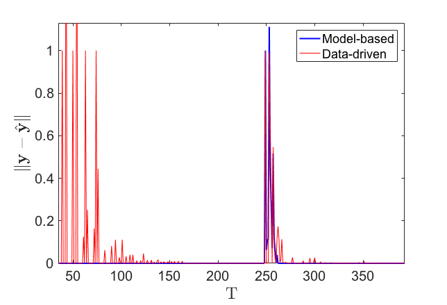
Figure 2: The figure shows the responses of the model-based and data-driven attack monitors for an attack input $u_{4}(249)=1$. Attack detection capability for the model-based monitor is achieved at time $T=15$ and for data-driven monitor at time $\bar{T}_{\text{safe}}=164$ (consistent with the result in Figure 1) as seen from the convergence to zero of the prediction error, implicitly validating Theorems II.1 and II.4. The attack is detected as an error in the output prediction by the monitors at $T=249$. We also observe that the data-driven monitor recovers from the attack at around $T=270$ when the prediction error is below $0.03$ units ($<3\%$ of attack input magnitude) and gradually decays to zero.

IV Conclusion and future work

In this letter, we characterized the fundamental limitations on data-driven monitoring of linear time-invariant systems from a systems-theoretic perspective. In particular: (i) we characterized an information bound on the output time series and the minimum time horizon length for measurement data collection to achieve detection capability; (ii) we provided a heuristic for the choice of dimensions of the Hankel matrix employed in data-driven attack detection; and (iii) we obtained a characterization of undetectable attacks. Surprisingly, our results show that model-based and data-driven detection strategies share the same limitations, thus relaxing the stringent assumption of the knowledge of the system dynamics that is typically made in existing security works.

Future work includes the limitations of data-driven detection in stochastic, time-varying and nonlinear systems.

Appendix A Proof of Theorem II.1

We have $\mathbf{w}(k+1)={S^{(\mathrm{m},\mathrm{nom})}}^{\top}\mathcal{O}_{N}x(k+1)={S^{(\mathrm{m},\mathrm{nom})}}^{\top}\mathcal{O}_{N}Ax(k)$. Suppose $x(k)\notin\mathrm{Ker}\left(\mathcal{O}_{N}\right)$, we get that $0\neq\mathcal{O}_{N}x(k)\in\mathrm{Col}\left(\mathcal{O}_{N}\right)=\mathrm{Col}\left(S^{(\mathrm{m},\mathrm{nom})}\right)$, and we can express $\mathcal{O}_{N}x(k)$ as a linear combination of the columns of $S^{(\mathrm{m},\mathrm{nom})}$. It then follows that ${S^{(\mathrm{m},\mathrm{nom})}}^{\top}\mathcal{O}_{N}x(k)\neq 0$. Moreover, if $x(k)\in\mathrm{Ker}\left(\mathcal{O}_{N}\right)$, then we have ${S^{(\mathrm{m},\mathrm{nom})}}^{\top}\mathcal{O}_{N}x(k)\neq 0$. Therefore, we get that $\mathrm{Ker}\left({S^{(\mathrm{m},\mathrm{nom})}}^{\top}\mathcal{O}_{N}\right)=\mathrm{Ker}\left(\mathcal{O}_{N}\right)$.

We note that $\mathbf{w}(k)\in\mathrm{Col}\left({S^{(\mathrm{m},\mathrm{nom})}}^{\top}\mathcal{O}_{N}\right)\cong\mathrm{Ker}^{\perp}\left({S^{(\mathrm{m},\mathrm{nom})}}^{\top}\mathcal{O}_{N}\right)$ for all $k\in\mathbb{N}$. We now express $x(k)\in\mathbb{R}^{n}=\mathrm{Ker}\left({S^{(\mathrm{m},\mathrm{nom})}}^{\top}\mathcal{O}_{N}\right)\oplus\mathrm{Ker}^{\perp}\left({S^{(\mathrm{m},\mathrm{nom})}}^{\top}\mathcal{O}_{N}\right)$ as $x(k)=\alpha(k)+\beta(k)$, where $\alpha(k)\in\mathrm{Ker}\left({S^{(\mathrm{m},\mathrm{nom})}}^{\top}\mathcal{O}_{N}\right)$ and $\beta(k)\in\mathrm{Ker}^{\perp}\left({S^{(\mathrm{m},\mathrm{nom})}}^{\top}\mathcal{O}_{N}\right)$. We have $\mathbf{w}(k)={S^{(\mathrm{m},\mathrm{nom})}}^{\top}\mathcal{O}_{N}x(k)={S^{(\mathrm{m},\mathrm{nom})}}^{\top}\mathcal{O}_{N}\beta(k)$. Since ${S^{(\mathrm{m},\mathrm{nom})}}^{\top}\mathcal{O}_{N}$ is a bijection from $\mathrm{Ker}^{\perp}\left({S^{(\mathrm{m},\mathrm{nom})}}^{\top}\mathcal{O}_{N}\right)$ to $\mathrm{Col}\left({S^{(\mathrm{m},\mathrm{nom})}}^{\top}\mathcal{O}_{N}\right)$, with ${\left({S^{(\mathrm{m},\mathrm{nom})}}^{\top}\mathcal{O}_{N}\right)}^{\dagger}$ as its inverse, we get that $\beta(k)={\left({S^{(\mathrm{m},\mathrm{nom})}}^{\top}\mathcal{O}_{N}\right)}^{\dagger}\mathbf{w}(k)$.

Now, we have $\mathbf{w}(k+1)={S^{(\mathrm{m},\mathrm{nom})}}^{\top}\mathcal{O}_{N}x(k+1)={S^{(\mathrm{m},\mathrm{nom})}}^{\top}\mathcal{O}_{N}Ax(k)={S^{(\mathrm{m},\mathrm{nom})}}^{\top}\mathcal{O}_{N}A\left(\alpha(k)+\beta(k)\right)={S^{(\mathrm{m},\mathrm{nom})}}^{\top}\mathcal{O}_{N}A\alpha(k)+{S^{(\mathrm{m},\mathrm{nom})}}^{\top}\mathcal{O}_{N}A\beta(k)={S^{(\mathrm{m},\mathrm{nom})}}^{\top}\mathcal{O}_{N}A\alpha(k)+{S^{(\mathrm{m},\mathrm{nom})}}^{\top}\mathcal{O}_{N}A{\left({S^{(\mathrm{m},\mathrm{nom})}}^{\top}\mathcal{O}_{N}\right)}^{\dagger}\mathbf{w}(k)$. Since $\alpha(k)\in\mathrm{Ker}\left({S^{(\mathrm{m},\mathrm{nom})}}^{\top}\mathcal{O}_{N}\right)=\mathrm{Ker}\left(\mathcal{O}_{N}\right)$, we have $CA^{i}\alpha(k)=0$ for all $i\in\{0,\ldots,N-1\}$. Now, if $N\geq\nu$, the observability index of the system (1), then we have $\mathrm{Rank}(\mathcal{O}_{N})=\mathrm{Rank}(\mathcal{O}_{N+1})$, and since $\mathrm{Ker}(\mathcal{O}_{N+1})\subseteq\mathrm{Ker}(\mathcal{O}_{N})$, it follows from the Rank-Nullity Theorem that $\mathrm{Ker}(\mathcal{O}_{N})=\mathrm{Ker}(\mathcal{O}_{N+1})$. We therefore get that $CA^{N}\alpha(k)=0$, which implies that $\mathcal{O}_{N}A\alpha(k)=0$, or in other words, $A\alpha(k)\in\mathrm{Ker}\left(\mathcal{O}_{N}\right)=\mathrm{Ker}\left({S^{(\mathrm{m},\mathrm{nom})}}^{\top}\mathcal{O}_{N}\right)$. This is equivalent to stating that the $\mathrm{Ker}\left({S^{(\mathrm{m},\mathrm{nom})}}^{\top}\mathcal{O}_{N}\right)$ is an invariant subspace of $A$ when $N\geq\nu$, the observability index of (1). Therefore, we get that $\mathbf{w}(k+1)=\left({S^{(\mathrm{m},\mathrm{nom})}}^{\top}\mathcal{O}_{N}\right)A{\left({S^{(\mathrm{m},\mathrm{nom})}}^{\top}\mathcal{O}_{N}\right)}^{\dagger}\mathbf{w}(k)$.

Appendix B Proof of Theorem II.4

We first recall that $Y_{N,T}=\mathcal{O}_{N}\left[\begin{matrix}x(0)&Ax(0)&\ldots&A^{T-N}x(0)\end{matrix}\right]=\left[\begin{matrix}\mathcal{O}_{N}x(0)&\mathcal{O}_{N}Ax(0)&\ldots&\mathcal{O}_{N}A^{T-N}x(0)\end{matrix}\right]$ We have $\mathbf{w}(k)=S^{\top}\mathcal{O}_{N}x(k)$ for all $k\in\mathbb{N}$. Let $x(k)=\alpha(k)+\beta(k)$, where $\alpha(k)\in\mathrm{Ker}\left(S^{\top}\mathcal{O}_{N}\right)$ and $\beta(k)\in\mathrm{Ker}^{\perp}\left(S^{\top}\mathcal{O}_{N}\right)$. We therefore get that $\mathbf{w}(k)=S^{\top}\mathcal{O}_{N}\beta(k)$. Since $S^{\top}\mathcal{O}_{N}$ is a bijection from $\mathrm{Ker}^{\perp}\left(S^{\top}\mathcal{O}_{N}\right)$ to $\mathrm{Col}\left(S^{\top}\mathcal{O}_{N}\right)$, we have that $\beta(k)=\left(S^{\top}\mathcal{O}_{N}\right)^{\dagger}\mathbf{w}(k)$.

Now, since $N\geq\nu$ and $T-N\geq\mu-1$, we get from Theorem II.3 that $Y_{N,T}$ is of maximum rank and we have $\mathbf{w}(k+1)=S^{\top}\mathcal{O}_{N}x(k+1)=S^{\top}\mathcal{O}_{N}Ax(k)=S^{\top}\mathcal{O}_{N}A\left(\alpha(k)+\beta(k)\right)=S^{\top}\mathcal{O}_{N}A\alpha(k)+S^{\top}\mathcal{O}_{N}A\left(S^{\top}\mathcal{O}_{N}\right)^{\dagger}\mathbf{w}(k)$.

Suppose $\alpha(k)\in\mathrm{Ker}\left(\mathcal{O}_{N}\right)$, and since $N\geq\nu$ we get that $\mathrm{Ker}\left(\mathcal{O}_{N}\right)$ is $A$-invariant, and we get that $A\alpha\in\mathrm{Ker}\left(\mathcal{O}_{N}\right)$, or in other words, $S^{\top}\mathcal{O}_{N}A\alpha(k)=0$. Now suppose, on the other hand, that $\alpha(k)\in\mathrm{Ker}^{\perp}\left(\mathcal{O}_{N}\right)\cap\mathrm{Ker}\left(S^{\top}\mathcal{O}_{N}\right)$, we would then indeed have $x(k)\in\mathrm{Ker}^{\perp}\left(\mathcal{O}_{N}\right)$. Moreover, let $V\subseteq\mathrm{Ker}^{\perp}\left(\mathcal{O}_{N}\right)$ be the smallest $A$-invariant subset of $\mathrm{Ker}^{\perp}\left(\mathcal{O}_{N}\right)$ containing $x(0)$. This implies that $x(k)\in V\subseteq\mathrm{Ker}^{\perp}\left(\mathcal{O}_{N}\right)$. Since the columns of $S$ form a basis of $\mathcal{O}_{N}V$, we get that $\mathcal{O}_{N}x(k)$ can be expressed as a linear combination of the columns of $S$, i.e., that $\mathcal{O}_{N}x(k)=Sv(k)$, with $v(k)\neq 0$ and we get $x(k)=\mathcal{O}_{N}^{\dagger}Sv(k)$. It then follows that $\mathcal{O}_{N}x(k)$ does not have a component orthogonal to all the column vectors of $S$, which implies that $\alpha(k)=0$ and we get a contradiction. Therefore, $\alpha(k)\notin\mathrm{Ker}^{\perp}\left(\mathcal{O}_{N}\right)\cap\mathrm{Ker}\left(S^{\top}\mathcal{O}_{N}\right)$. Thus, we get that $\mathbf{w}(k+1)=\left(S^{\top}\mathcal{O}_{N}\right)A\left(S^{\top}\mathcal{O}_{N}\right)^{\dagger}\mathbf{w}(k)$. and we can write $\vec{W}=\left(S^{\top}\mathcal{O}_{N}\right)A\left(S^{\top}\mathcal{O}_{N}\right)^{\dagger}W$. It is clear from the above that $\mathrm{Col}\left(\vec{W}^{\top}\right)\subseteq\mathrm{Col}\left(W^{\top}\right)$, from which we infer that $\left(S^{\top}\mathcal{O}_{N}\right)A\left(S^{\top}\mathcal{O}_{N}\right)^{\dagger}=\vec{W}W^{\dagger}$ is the global minimizer for the minimization problem (7) and that the minimum value is zero.

References

• [1] A. A. Cárdenas, S. Amin, and S. S. Sastry. Research challenges for the security of control systems. In Proceedings of the 3rd Conference on Hot Topics in Security, pages 6:1–6:6, Berkeley, CA, USA, 2008.
• [2] F. Pasqualetti, F. Dörfler, and F. Bullo. Attack detection and identification in cyber-physical systems. IEEE Transactions on Automatic Control, 58(11):2715–2729, 2013.
• [3] Y. Chen, S. Kar, and J. M. F. Moura. Dynamic attack detection in cyber-physical systems with side initial state information. IEEE Transactions on Automatic Control, 62(9):4618–4624, 2016.
• [4] S. Papadimitriou, J. Sun, and C. Faloutsos. Streaming pattern discovery in multiple time-series. In Proc. of the 31st International Conference on Very Large Data Bases, pages 697–708, 2005.
• [5] D. Shi, Z. Guo, K. H. Johansson, and L. Shi. Causality countermeasures for anomaly detection in cyber-physical systems. IEEE Transactions on Automatic Control, 63(2):386–401, 2017.
• [6] R. Hink, J. M. Beaver, M. A. Buckner, T. Morris, U. Adhikari, and S. Pan. Machine learning for power system disturbance and cyber-attack discrimination. In 7th International Symposium on Resilient Control Systems, pages 1–8, 2014.
• [7] M. Kravchik and A. Shabtai. Detecting cyber attacks in industrial control systems using convolutional neural networks. In Proc. of the ACM Workshop on Cyber-Physical Systems Security and Privacy, pages 72–83, 2018.
• [8] J. Inoue, Y. Yamagata, Y. Chen, C. M. Poskitt, and J. Sun. Anomaly detection for a water treatment system using unsupervised machine learning. In IEEE International Conference on Data Mining Workshops, pages 1058–1065, 2017.
• [9] J. Goh, S. Adepu, M. Tan, and Z. S. Lee. Anomaly detection in cyber physical systems using recurrent neural networks. In IEEE 18th International Symposium on High Assurance Systems Engineering (HASE), pages 140–145, 2017.
• [10] J. C. Willems, P. Rapisarda, I. Markovsky, and B. L. M. De Moor. A note on persistency of excitation. Systems & Control Letters, 54(4):325–329, 2005.
• [11] H. J. Van Waarde, J. Eising, H. L. Trentelman, and M. K. Camlibel. Data informativity: a new perspective on data-driven analysis and control. IEEE Transactions on Automatic Control, 2020.
• [12] C. De Persis and P. Tesi. Formulas for data-driven control: Stabilization, optimality and robustness. IEEE Transactions on Automatic Control, 65(3):909–924, 2020.
• [13] G. Baggio, V. Katewa, and F. Pasqualetti. Data-driven minimum-energy controls for linear systems. IEEE Control Systems Letters, 3(3):589–594, 2019.
• [14] Y. Liu, P. Ning, and M. K. Reiter. False data injection attacks against state estimation in electric power grids. ACM Transactions on Information and System Security, 14(1):1–33, 2011.
• [15] Y. Mo and B. Sinopoli. False data injection attacks in electricity markets. In IEEE Int. Conf. on Smart Grid Communications, pages 226–231, Gaithersburg, MD, October 2010.
• [16] R. A. Horn and C. R. Johnson. Matrix Analysis. Cambridge University Press, 1985.
• [17] M. Sain and J. Massey. Invertibility of linear time-invariant dynamical systems. IEEE Transactions on Automatic Control, 14(2):141–149, 1969.
• [18] J. H. Tu, C. W. Rowley, D. M. Luchtenburg, S. L. Brunton, and J. N. Kutz. On dynamic mode decomposition: Theory and applications. Journal of Computational Dynamics, 1(2):391–421, 2014.
• [19] J-N. Juang and R. S. Pappa. An eigensystem realization algorithm for modal parameter identification and model reduction. Journal of Guidance, Control and Dynamics, 8(5):620–627, 1985.