Getting to 99% Accuracy in Interactive Segmentation

Abstract

Interactive object cutout tools are the cornerstone of the image editing workflow. Recent deep-learning based interactive segmentation algorithms have made significant progress in handling complex images and rough binary selections can typically be obtained with just a few clicks. Yet, deep learning techniques tend to plateau once this rough selection has been reached. In this work, we interpret this plateau as the inability of current algorithms to sufficiently leverage each user interaction and also as the limitations of current training/testing datasets.

We propose a novel interactive architecture and a novel training scheme that are both tailored to better exploit the user workflow. We also show that significant improvements can be further gained by introducing a synthetic training dataset that is specifically designed for complex object boundaries. Comprehensive experiments support our approach, and our network achieves state of the art performance.

O45 O1em m #3

1 Introduction

Interactive image segmentation aims at generating a binary mask that delineates a foreground object of interest from the background. Unlike in semantic image segmentation, user interactions are expected and must be exploited. Typically, the interaction will come in the form of clicks that the user will place to fix errors in foreground or background areas. In an ideal interactive session, the main shape is sketched in a few clicks, then smaller local details are refined with subsequent edits. Exploring and exploiting this interactive editing loop is the objective of this paper.

Classic approaches to interactive segmentation [1, 2, 3] have found some use in professional applications like Photoshop. Artists require a tool which is responsive to their edits and flexible enough to allow for a wide range of shapes. The work of Liu et al. [4] (2009) is particularly interesting in that regard, as they acknowledge the progressive nature of image editing and pay particular attention to the artist workflow. For instance, they make sure that changes to the mask stay localised to the user edit, so as not to undo progress. These early works have however poor performance on textured regions, and some images may require many clicks just to get a rough selection.

Recently, deep-learning approaches have excelled at producing rough segmentation masks with minimal user input. Object masks can now be typically be extracted to 90% accuracy(mean Intersection over Union/mIoU [5]) in under six clicks [6, 7, 8, 9, 10, 11, 12, 13], even on highly textured images. A caveat of its successes; deep-learning approaches are also observed to plateau short of 95% accuracy, even after 10 or more clicks and are unable to output very detailed masks, even after 20 clicks.

Such low-resolution predictions may be sufficient for casual applications, such as dataset annotation. For professional high-end applications, such as Photoshop, this is of little interest as professional artists can manually draw 90% accurate masks in no time. What they really need is a tool to help them reach 99-100% accuracy reliably. See Figure 1 for a comparison of results achieving 90% [8] accuracy and our results which achieve 99%.

One reason for this plateau is that current architectures manipulate images and click interactions at low resolution, while fine details are usually only recovered through post-processing stages (either using graph cuts [6, 13] or CNNs [14, 10]). This is partly a consequence of existing benchmarks having set low accuracy targets for the task [6]: in the Berkeley benchmark[15] the threshold is set to 90% accuracy, 90% for the GrabCut dataset [16] and only 85% for PASCAL [5]. These arbitrary targets come from a focus on quick rough selections and imperfections in the manual delineations of the objects when creating the ground-truth labelling. Any pixel within 3-5 pixels of the object boundary is typically ignored in the evaluation. As a result, it was noted in FCN [17] that working at $8\times$ lower resolution yields sufficient accuracy for the benchmark tasks of semantic segmentation, and many deep learning architectures are content working at $8\times$ or $4\times$ lower output resolution than the original image [6, 7, 8, 9, 12].

Figure 1: Comparison between state of the art segmentation at 90% accuracy [8] and our results (right) at 99% accuracy.

Another reason for the plateau is that current approaches treat all user interactions the same. During training, a set of foreground and background clicks are typically placed on the object and background, according to heuristic strategies [8, 10, 11, 12, 13, 7]. These clicks are placed together during training, without keeping any state or order information from one interaction to the next. The networks are thus not specifically trained to respond to corrective user clicks. Only in [18, 7] was the idea of training the network one edit at a time was explored, but only after that a good initial segmentation is given. There is thus a need to better focus on the way artists approach iterative segmentation and how to respond precisely to their input.

The primary objective of this paper is to reach higher levels of segmentation accuracy by working at full resolution and modelling, from the start, the selection process as a series of interactions, whose purpose shifts over time from identifying the object globally to refining it locally. To achieve that goal, we are making a series of contributions covering all aspects of the problem. These contributions include:

1. A single architecture which allows for high resolution processing. The core architecture is based on a U-Net style decoder with skip connections to handle fine details. We further incorporate a Guided Filter layer [19] to refine the results and produce precise transparency masks.

2. Our architecture is split across two encoding streams: an Image stream and an Interaction stream. This separation of the inputs improves the propagation of the user interactions throughout the network and helps precisely respond to each click.

3. A training strategy where the corrective clicks are sequentially added from the first click, so as to match the artist workflow and thus jointly train for initial rough segmentation and detailed refinements.

4. Demonstrating that a high quality synthetic dataset, specifically designed to target fine details, can be used to further improve the quality of the segmentation.

The proposed method achieves state of the art performance for any number of clicks and can reach 99% accuracy for 62% of images at 20 clicks. More importantly, it is also demonstrably more usable for artists, as the network predictions are more predictable and easier to subsequently edit.

The rest of the paper is organised as follows. In Section 2 we review prior works related to our approach. In Section 3 we detail our proposed method. In Section 4 we compare our method to the state of the art algorithms and we perform ablation experiments to quantitatively and qualitatively assess our contributions. In Section 5 we present our new training synthetic dataset and study how it can impact the quality of the segmentation.

2 Related Works

In recent years, deep-learning based approaches to interactive segmentation (e.g. [6, 14, 13]) have superseded prior works [3, 4, 1, 2]. While the core architecture of interactive segmentation networks is typically borrowed from semantic segmentation networks (e.g. DeepLab [20]), or general purpose image processing architectures (e.g. U-Net [21]), deep interactive segmentation requires addressing two specific challenges: 1) how to best encode the sequence of user interactions in the architecture and 2) how to train the network so as to best match the behaviour of artists. In the rest of this section, we look at how existing works approach the design and training of interactive segmentation networks.

2.1 Segmentation Architectures

Most previous interactive segmentation networks are either based on semantic segmentation networks, such as DeepLab [20], or general purpose image processing networks such as U-Net [21]. Semantic Segmentation networks typically follow an Encoder-Decoder architecture and use off-the-shelf encoders pretrained on ImageNet [22]. For instance, the works of Xu et al. [6] and Majumder and Yao [12] are based on the FCN semantic segmentation network of Shelhamer et al. [17], which itself is based on the ImageNet trained VGG16 network of Simonyan and Zisserman [23]. The differences between notable prior works on Interactive Segmentation are included in Tables 1,  2 and 3.

Note that techniques based on semantic segmentation networks typically operate at $\nicefrac{{1}}{{4}}$ or $\nicefrac{{1}}{{8}}$ resolution, which is a too low resolution for our aim. Full resolution output can be obtained by using Graph-Cuts (see iFCN [6], RIS-Net [13]) or by appending a dedicated upsampling networks (see FCTSFN [10] and BRS [14]). Upsampling networks need to be trained afterwards, in a two-stage process. In RIS-Net [13], fullres prediction is obtained by fusing the predictions of two decoder streams: the first stream makes a global low resolution prediction and the second stream independently processes patches at click locations to give local hires predictions. In IIS-LD [11], a single full resolution network is proposed by using VGG hypercolumns.

Name	Reference	Encoder	Decoder	Scale	Post-Processing
iFCN	Xu et al. [6]	VGG16 [23]	FCN [17]	1:8	graph-cuts [1]
ITIS	Mahadevan et al. [7]	Xception [24]	DeepLab-v3+ [25]	1:4	none
DEXTR	Maninis et al. [8]	ResNet-101 [26]	Deeplab-v2	1:8	none
VOS-wild	Benard et al. [9]	ResNet-101	Deeplab-v2 [27]	1:8	CRF [28]
FCTSFN	Hu et al. [10]	VGG16	CNN with bilinear upsampling	1:1	refinement network
IIS-LD	Li et al. [11]	VGG16	hypercolumn, CAN [29]	1:1	none
CAMLG	Majumder et al. [12]	VGG16	FCN	1:8	none
RIS-Net	Liew et al. [13]	VGG16	DeepLab-LargeFOV [27], custom CNN for local predictions around clicks	1:1	graph-cuts
IITSEN	Bredell et al. [18]	U-Net [21]	U-Net	1:1	none
BRS	Jang and Kim [14]	DenseNet [30]	U-Net	1:1	refinement network
Ours	-	ResNet-50, groupnorm [31], weight standardisation [32]	Pyramid Pooling [33],U-Net	1:1	guided filter layer [34]

Table 1: Segmentation Architecture in relevant previous works, detailing: the type of decoder and encoder used, the scale of the tensor after the decoder and the post-processing method used for upsampling the results to full resolution.

Name	Reference	Click Embedding	Click Fusion	Feedback Fusion
iFCN	Xu et al. [6]	Distance Map	early	none
ITIS	Mahadevan et al. [7]	Gaussian	early	early
DEXTR	Maninis et al. [8]	Gaussian	early	none
VOS-wild	Benard et al. [9]	Gaussian	early	none
FCTSFN	Hu et al. [10]	Distance Map	late	none
IIS-LD	Li et al. [11]	Gaussian	late	none
CAMLG	Majumder et al. [12]	Superpixel based embedding [12]	early	optional
RIS-Net	Liew et al. [13]	Distance Map	early	none
IITSEN	Bredell et al. [18]	Distance Map	early	early
BRS	Jang and Kim [14]	Distance Map	early	none
Ours	-	Gaussians at 3 Scales [35]	both	late

Table 2: User Interactions Encoding in relevant previous works.

Name	Reference	Loss	Training Schedule	Training Dataset
iFCN	Xu et al. [6]	BCE	all clicks at once	PASCAL 2012
ITIS	Mahadevan et al. [7]	BCE	adding one click per epoch	SBD Training + PASCAL 2012
DEXTR	Maninis et al. [8]	BCE	4 boundary clicks at once	SBD Full
VOS-wild	Benard et al. [9]	BCE	all clicks at once [6]	SBD Full
FCTSFN	Hu et al. [10]	BCE	all clicks at once [6]	PASCAL 2012
IIS-LD	Li et al. [11]	IoU + click location	all clicks at once [6]	SBD Training
CAMLG-IIS	Majumder et al. [12]	BCE	all clicks at once [6]	SBD Full
RIS-Net	Liew et al. [13]	BCE + Click Discounting [13]	all clicks at once [6]	PASCAL 2012
IITSEN	Bredell et al. [18]	BCE	Separate network makes initial prediction, then adding clicks per image.	Medical [36]
BRS	Jang and Kim [14]	BCE	all clicks at once[14]	SBD Training
Ours	-	IoU + click location	adding clicks per image from scratch	SBD Training + Synthetic

Table 3: Loss and Training in relevant previous works.

2.2 Embedding User Interactions

Encoding the Clicks

The core segmentation network also needs to be adapted to include the user interactions. In the literature, interactions come in the form of clicks: positive clicks indicate foreground regions and negative clicks background regions. Such click inputs are encoded as images either via a distance transform [6, 13, 18, 10, 12] or by fitting Gaussian masks to each of the clicks [8, 35, 9, 11].

To integrate the click maps into the network, most papers (iFCN [6], RIS-Net [13], ITIS [7], DEXTR [8]) adopt an early fusion scheme by simply joining the click maps as extra channels to the input image tensor. Later fusion schemes are however possible. In IIS-LD [11], the click maps are concatenated with all the upsampled image features hypercolumn. In FCTSFN (Hu et al. [10]), VGG16 is applied separately to both the input image and the click maps. The lower resolution features from both inputs are then concatenated before being passed to further convolutional layers. They show that the late feature fusion of click and image streams out-performs concatenation of image and clicks at the beginning of a single stream.

2.2.1 Mask Predictions Feedback

In most prior works (including iFCN [6], RISNET [13], DEXTR [8], IIS-LD [11], FCTSFN [10]), when a user adds a new click, the previous prediction is discarded and a new prediction is make afresh. This means no state is carried on from one click to the next. We could try, however, to learn from previous clicks and predictions as they give more context to what the new click is trying to fix. The approach proposed in ITIS by Mahadevan et al. [7] and IITSEN by Bredell et al. [18] is to feed back the mask alongside the image and the clicks (early fusion) in order to retain some state information.

One potential issue with this early fusion approach is that it might be hard for the network to recover from a very poor previous prediction.

2.3 Training Scheme

The specificity of training interactive segmentation models is that user clicks need to be supplied during training. As it is impractical to provide human-generated clicks, the clicks must be simulated in some way. How best to do this is an open question.

In their early work on deep interactive segmentation, Xu et al. [6] use a set of three strategies for generating clicks from a given segmentation label. The method goes as follows: a random number of foreground clicks are placed randomly on the object and a random number of background clicks are placed near the object. This sampling strategy seeks to mimic typical human input patterns and it has been adopted by many subsequent works [10, 35, 11, 12, 9, 13].

Mahadevan et al. [7] (ITIS) observe, however, that this way of predetermining the click placements, independently of the network prediction errors, has an adverse impact on the final model accuracy. They propose to start with this scheme at first, but then, at each subsequent epoch, a new click is added on the centre of the largest incorrect region. This training scheme tries to increase the correlation between the click locations and prediction errors. The issue is that the initial click samples are still randomly grouped. Also, later clicks are only updated one epoch at a time but the network weights may have changed significantly between each epoch. This means that the click sequences are not necessarily coherent.

A more direct approach for training interactive image segmentation networks was taken by Bredell et al. [18] for medical image segmentation. After an initial segmentation is computed by a separate network, the interactive network is trained by iteratively adding one click at a time. Each click is placed on the largest incorrect region. The approach, however, still relies on an initial segmentation, which we believe is unnecessary.

3 Proposed Approach

3.1 An Interactive Hi-Resolution Network Architecture

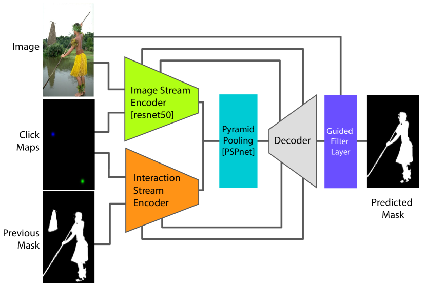
Figure 2: Proposed Architecture. The Image Stream generates image features using ResNet-50, whereas the Interaction Stream embeds the previous mask estimate and the user clicks. Both streams get fused and pass through the pyramid pooling. The decoder follows a U-Net style architecture. The final layer is a $5\times 5$ Deep Guided Filter layer, which allows for fine details extraction.

	Figure 3: Comparison of mean IoU scores after $n$ clicks for the GrabCut testset [16].
	Figure 4: Comparison of mean IoU scores after $n$ clicks for the Berkeley testset [15].
	Figure 5: Comparison of mean IoU scores after $n$ clicks for the SBD testset [37].

The proposed architecture is presented in Figure 2. The segmentation masks are achieved through the use of an encoder-decoder network. One key aspect of our model is that we split the input image and user interactions into two streams: the Image stream and the Interaction stream. The separation into two streams is designed to allow for both early and late fusion approaches and thus better respond to user interactions.

Our approach differs in some key ways from prior methods which have used the previous mask as input to the network [18, 7] and methods which separate the streams for clicks and the image [10]. Firstly, we adopt a late fusion for integrating the mask to the image stream. By using a separate branch, we prevent poor previous mask estimates from affecting the computation of the image features, while still allowing the mask information to be used. Secondly, we feed the clicks to both the image and interaction stream, which we observed to improve accuracy, as opposed to using early or late fusion alone.

The Image Stream architecture is based on ResNet-50 with Group Normalisation and Weight Standardisation [32]. The weights are initialised by pre-training on ImageNet for classification [32]. Two modifications are made to the network. First, we increase the number of input channels from 3 to 9 to allow for the extra click input maps. We encode the foreground and background clicks as in [35] using Gaussian masks at three different scales, centred on each click. Second, we remove the striding from ‘layer 3’ and ‘layer 4’ of ResNet-50 and increase the dilation to 2 and 4 respectively. This increases the output resolution from the Image Stream by 4 times. We experimented with replacing ResNet-50 with ResNet-101 or ResNet-101 pretrained for semantic segmentation, but we did not observe any noticeable improvement.

Because our training regime requires a batch size of 1, a crucial tweak is that we use Group Normalisation (GN) [31] (32 channels per group) with Weight Standardisation [32] instead of Batch Normalisation.

The Interaction Stream encodes the previous mask together with the click maps. It has six convolutional layers (see Table 4), each followed by the LeakyReLu activation function [38]. Three of the layers are strided convolutions with stride two, so the output resolution matches that of the Image Stream.

The Decoder concatenates features from both streams and passes them to a Pyramid Pooling layer [33]. The pooled features are fed into a decoder which contains eight convolutional layers interleaved with three bilinear upsampling layers and skip connections from both streams (see Table 5). The output of the decoder is at full resolution.

Fine Details are then extracted by appending a Guided Filter layer [34]. This further refines the mask details and allow us to obtain a transparency mask that can capture subpixel features, such as hair strands, as well as transparency, such as in motion blur. This means that the predicted mask is now a proper transparency mask that can be subsequently used for compositing the selected object onto a different background.

The full implementation details of the network architecture can be found on the project page.

Interaction Stream Encoder Layer	X	C	S
Concat: Clicks & Previous Mask	256	7	-
conv1	256	64	1
conv2	128	128	2
conv3	128	256	1
conv4	64	256	2
conv5	32	256	2
conv6	32	256	1

Table 4: Network architecture for the Interaction Stream Encoder. X is the output spatial resolution, C is output number of channels, S is the convolution stride. All convolutional layers are followed by LeakyRelu activations [38].

Decoder Layer	X	C	GN	Up
Concat: Features from PPM & Interaction Stream ‘conv6’	32	3328
conv1	32	256	✓
conv2	32	256	✓	✓
Concat: ResNet ‘layer 1’ & Interaction Stream ‘conv4’	64	768
conv3	64	256	✓	✓
Concat: ResNet ‘conv 3’ & Interaction Stream ‘conv2’	128	384
conv4	128	64	✓	✓
Concat: Image & Clicks	256	73
conv5	256	32
conv6	256	16
conv7: (1x1, clip(0,1))	256	1

Table 5: Network architecture for the decoder. X is the output spatial resolution, C is output number of channels, GN indicates if the LeakyReLu was followed by a Group Normalisation  [31] layer, Up indicates if the layer was followed by 2x bilinear upsampling. All convolutional layers except ‘conv7’ are followed by LeakyReLu activations.

3.2 Training

Training Schedule

A fundamental deviation from previous works is that we train our network, image by image, click by click. Whereas in prior works the clicks are first bundled together, we propose to introduce the clicks sequentially, starting from a single click, and adopting the same sequential scheme used to evaluate interactive segmentation algorithms [39, 6, 13, 11, 35, 12, 9, 10]. For each click, we first look at the previously predicted map, and segment the mislabelled pixels into connected regions. We place the click at the centre of the largest incorrect region, so as to maximise the Euclidean distance to both the region boundary and the sides of the image. For the first click, the prediction map is set to zero. The loss is then computed after the placement of each click and the weights are updated through back-propagation before the next click.

By iterating through each click, we are essentially combining the loss for the entire range of clicks, hence effectively computing the area under the accuracy per clicks curve (as seen in Figures 5, 5 and 5). This has the advantage that our training loss matches the final metric used for evaluation. Also, this means that we are optimising for the whole range of clicks. In practice we found that using 4 clicks per image was optimal. The overall performance did not improve when placing more than 4 clicks but started to degrade when using 3 or less clicks.

Loss

The loss for a particular image is defined, as in Li et al. [11] (IIS-LD), as the sum of the soft-IoU loss and a click location loss:

$$L(\alpha)=1-\frac{\sum_{i}\alpha_{i}\hat{\alpha}_{i}}{\sum_{i}\max(\alpha_{i},\hat{\alpha}_{i})}+\sum_{c\in\mathrm{Clicks}}\left(\alpha_{c}-\hat{\alpha}_{c}\right)^{2}$$ (1)

where $\alpha_{i}$ and $\hat{\alpha}_{i}$ are the mask prediction and ground truth mask values at pixel $i$. We found that using the soft-IoU led to visually and quantitatively better results than when using the binary cross entropy (BCE) loss. Segmentation results with BCE tend to show more spurious isolated regions than with the soft-IoU loss.

Hyper-Parameters

The ResNet-50 is initialised by pre-training on ImageNet [32]. We train our model with the RAdam optimiser [40] with a learning rate of $10^{-5}$, with a single image in each batch. The learning rate is reduced by a factor of 0.1 at epochs 14, 17 and 20, and training completes after 25 epochs. We apply weight decay of $0.005,10^{-5}$ to convolutional weights, and the GN parameters respectively. Images are cropped at a fixed size of $352\times 352$ pixels, and we use horizontal flipping, gamma augmentations, and brightness augmentations.

4 Evaluation

4.1 Benchmarks

We evaluate our work across three publicly available segmentation datasets. GrabCut [16] is a 50 image dataset with 50 ground truth masks, although pixels in a thin band around the object boundaries are not labelled. Berkeley [15] is a 96 image dataset with 100 ground truth masks, the masks are of the highest quality of all three datasets. SBD [37] validation set contains 2,820 images with multiple labels per image. The labels span 20 object classes.

4.2 Comparison to the State of the Art

Method	GrabCut NoC @ 90%	Berkeley NoC @ 90%	SBD NoC @ 85%
IFCN [6]	6.04	8.65	9.18
RIS-Net [13]	5.00	6.03	-
ITIS [7]	5.60	-	-
DEXTR [8]	4.00	-	-
VOS-wild [9]	3.8	-	-
FCTSFN [10]	3.76	6.49	-
IIS-LD [11]	4.79	-	7.41
CAMLG-IIS [12]	3.58	5.60	-
BRS [14]	3.6	5.08	6.59
Ours	2.54	3.53	3.90

Table 6: The mean number of clicks required to achieve a certain mIoU accuracy on different datasets [16, 15, 37] by various algorithms. The best results are indicated in bold with the second best underlined.

In this section, we use two metrics to demonstrate the superior performance of our algorithm over existing work.

Quick Selection. On Table 6 we report the mean number of clicks that it takes to reach the customarily used 85%/90% IoU threshold, known as the Number of Clicks metric(NoC @ $x$%). Our algorithm reaches 90% accuracy in 2.54 clicks on GrabCut and 3.53 clicks on Berkeley. It reaches 85% in 3.90 clicks on the SBD test set. These are all significant improvements over the state of the art.

We primarily use this metric in order to compare with results reported from previous methods. As seen in Figure 1 the segmentation quality at 90% is not sufficient for image editing, and as seen in Figures 5–5 many methods plateau in accuracy around those thresholds. So we believe it is more important to measure accuracy for a wide range of clicks.

Accuracy per Click. On Figures 5–5 is reported the average segmentation accuracy (mean IoU) across the first 20 iterated clicks for state of the art algorithms on each dataset. The click placement strategy used in the evaluation is the same used by all other methods. In the legend we also report the area under curve (AuC) score across the full range of clicks (1-20). From the graph and the AuC score we see that our algorithm outperforms all others, on all datasets, for every number of clicks. On the GrabCut graph we see that for the first click our method matches the accuracy of CAMLG-IIS [12] yet their method does not make good use of the corrective clicks compared to ours. We believe the AuC metric is much more relevant for future works than the number of clicks, hence we use it for our ablation study. The graphs show there is still large room for improvement in future work for both at early clicks and for reducing the plateau at later clicks, especially on the Berkeley and SBD datasets.

4.3 Ablation Study

We study the effectiveness of our contributions for the following scenarios:

• A baseline model for our method is based on the Image stream, pyramid pooling layer and decoder alone and does not include the Interaction Stream nor the Guided Filter Layer. It is trained using the standard bundled click strategy from Ning et al. [6].

• In ($+T$), we change the training approach to our click by click iterative training scheme.

• In ($+T,+I$), we also include the Interaction Stream ($+I$), without the previous mask feedback (i.e. it is set to zero).

• In ($+T,+I,+F$), the previous predicted mask is fed to the Interaction Stream.

• In ($+T,+I,+F,+G$), our full model is completed by appending a Guided Filter Layer. Unless otherwise stated all results in this paper refer to this model.

Accuracy per Click. On Figures 9, 9 and 9 are reported the mean IoU across the range of 20 clicks on the SBD dataset [37]. The area under the curve, with its confidence interval, is also compiled in Table 7. We plot the results from the state of the art method BRS [14] as a reference.

We can see that our stripped down baseline model performs about on par with the state of the art, which points to the strength of our ResNet-50 based Encoder Decoder architecture with Group Normalisation. Then, training the model with our interactive regime ($+T$) gives a clear boost to accuracy for all clicks. Then adding the interactive stream ($+T,+I$) gives a consistent improvement at higher numbers of clicks, where fine edits are made. Similarly, adding the feedback of the mask ($+T,+I,+F$) improves results for later clicks on all three datasets. The Guided Filter layer gives improvements on the Grabcut [16] and Berkeley [15] datasets but not on the SBD [37] set. We believe this is because the labels on SBD do not follow the object boundaries closely (see discussion in section 5), but Guided Filter refines the prediction based on the image edges.

Method	GrabCut	Berkeley	SBD
ours: baseline	$0.9121\pm 0.0078$	$0.9065\pm 0.0036$	$0.8416\pm 0.0008$
ours:$+T$	$0.9516\pm 0.0041$	$0.9306\pm 0.0022$	$0.8842\pm 0.0006$
ours:$+T,I$	$0.9486\pm 0.0038$	$0.9350\pm 0.0019$	$0.8941\pm 0.0005$
ours:$+T,I,F$	$0.9625\pm 0.0031$	$0.9396\pm 0.0018$	$0.9079\pm 0.0005$
ours:$+T,I,F,G$	$0.9628\pm 0.0025$	$0.9423\pm 0.0018$	$0.9026\pm 0.0005$

Table 7: Mean IoU for the 1-20 clicks range on the different datasets [16, 15, 37] for each variant of our algorithm.

Corrective Click Accuracy. On Figure 6, we introduce a novel way to measure interactive segmentation performance. At each click iteration, we measure the proportion of correctly predicted pixels within the previous incorrect region, which is where this new click was placed. In effect, this measures the networks ability to accurately respond to user inputs, something very important for the user experience. We compare on Berkeley our baseline model to the one with interactive training and the full model, which also includes the Guided Filter Layer, and the interaction stream with mask feedback.

Interestingly, all three methods perform equally for the first three clicks. However, the baseline model continuously drops in corrective accuracy after this. The more clicks are added, the less it responds to each click. Our interactive training improves this and has much higher corrective accuracy for all clicks, but it still drops over time. Our full model maintains a steady 50% corrective accuracy for each click, indicating it more consistently leverages each user input.

Figure 6: Correction accuracy at each click for the Berkeley dataset [15]. The correction accuracy is defined as the proportion of pixels correctly predicted on the region where the click was placed (see text).

	Figure 7: Comparison of mean IoU scores after $n$ clicks for the GrabCut testset [16].
	Figure 8: Comparison of mean IoU scores after $n$ clicks for the Berkeley testset [15].
	Figure 9: Comparison of mean IoU scores after $n$ clicks for the SBD testset [37].

Reaching 99% accuracy On Figures 12, 12 and 12 we plot the proportion of images where the prediction accuracy surpasses 90-99% accuracy at 1,5,10 and 20 clicks. We see that by adding more clicks we not only raise the lower bar of accuracy but also the number of images reaching 99%. At 20 clicks, 100% of images exceed 95% accuracy, and 62% of images exceed $99\%$ accuracy on the GrabCut dataset. The Berkeley and SBD datasets are more difficult, yet at 20 clicks our method still exceeds 95% accuracy for 81% and 55% respectively.

	Figure 10: Proportion of images surpassing $x\%$ accuracy after $n$ clicks for the GrabCut testset [16]. 62% of predictions exceed $99\%$ accuracy after 20 clicks.
	Figure 11: Proportion of images surpassing $x\%$ accuracy after $n$ clicks for the Berkeley testset [15]. 81% of predictions exceed $95\%$ accuracy after 20 clicks.
	Figure 12: Proportion of images surpassing $x\%$ accuracy after $n$ clicks for the SBD testset [37]. 55% of predictions exceed $95\%$ accuracy after 20 clicks.

4.4 Qualitative Evaluation

In Figure 14 and 15 we compare the predictions of our baseline and full algorithms for six clicks on images from the GrabCut and Berkeley datasets. Note that the baseline approach sometimes fails to recover from poor initial guesses, whereas our iteratively trained network is better at correcting with each click.

In Figure 13 we see that, after 20 clicks, both models roughly select the object, but our final model is visibly more precise in these instances.

To illustrate the behaviour of our method across the whole range of difficulties, we sampled in Figure 16 images based on their accuracy at 20 clicks. The images are ranked from easiest (top) to hardest (bottom).

BL
Ours

Figure 13: Qualitative comparison between our baseline and our model after 20 clicks. Object masks are highlighted in cyan.

	Click 1	Click 2	Click 3	Click 4	Click 5	Click 6
BL
Ours
BL
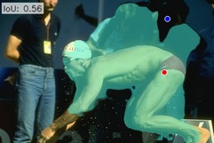
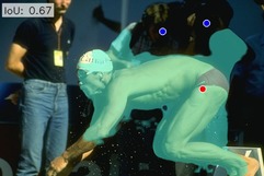
Ours
BL
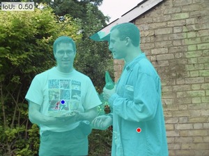
Ours
BL
Ours

Figure 14: Qualitative comparison between our baseline (BL) and our model across the first 4 clicks. Positive clicks are in red, negative in blue, object masks are highlighted in cyan. Images are from the GrabCut Dataset.

	Click 1	Click 2	Click 3	Click 4	Click 5	Click 6
BL
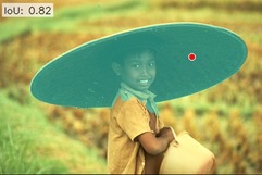
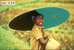
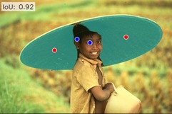
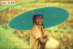
Ours
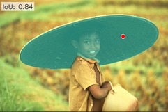
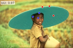
BL
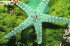
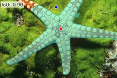
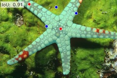
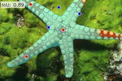
Ours
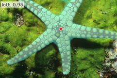
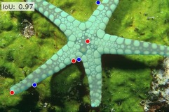
BL
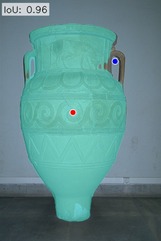
Ours
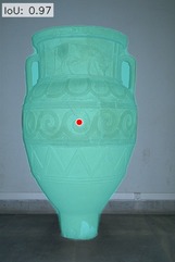
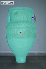
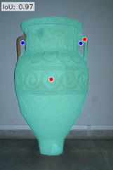
BL
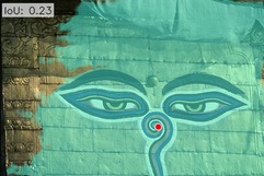
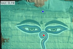
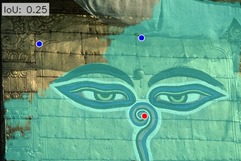
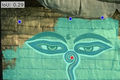
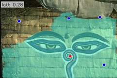
Ours

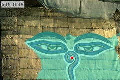
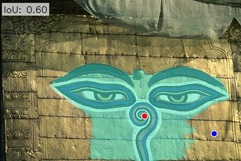
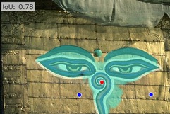
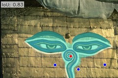
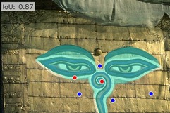
Figure 15: Qualitative comparison between our baseline (BL) and our model across the first 6 clicks. Positive clicks are in red, negative in blue, object masks are highlighted in cyan. Images are from the Berkeley Dataset.

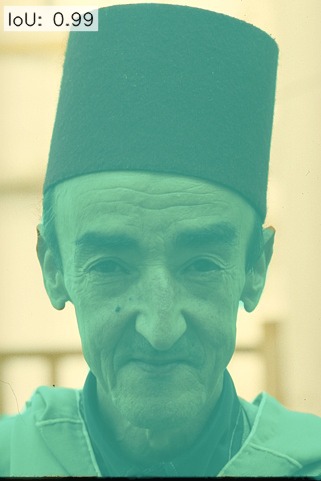
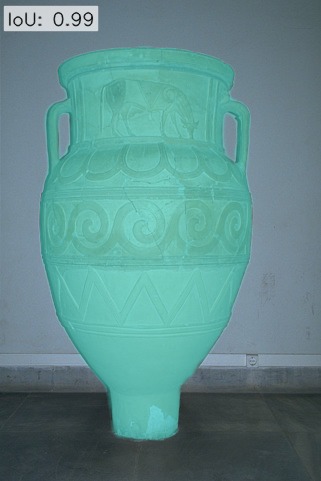
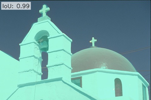
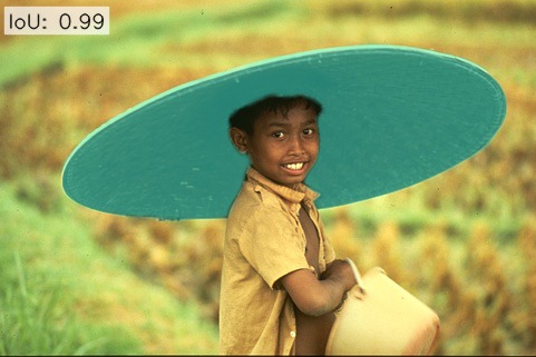
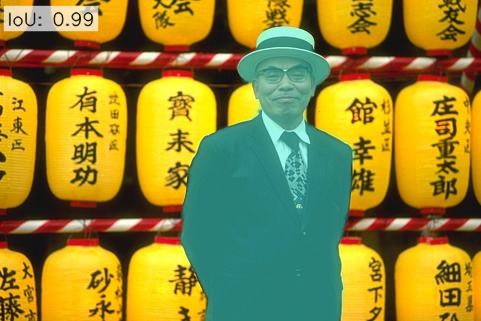
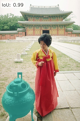
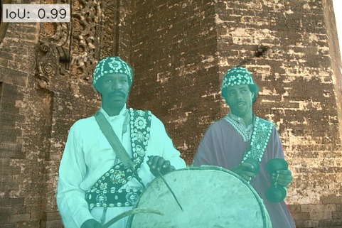
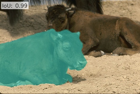
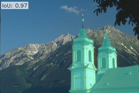
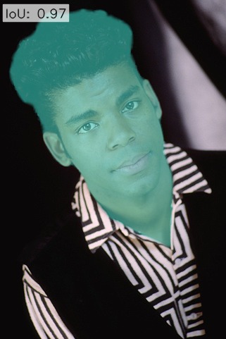
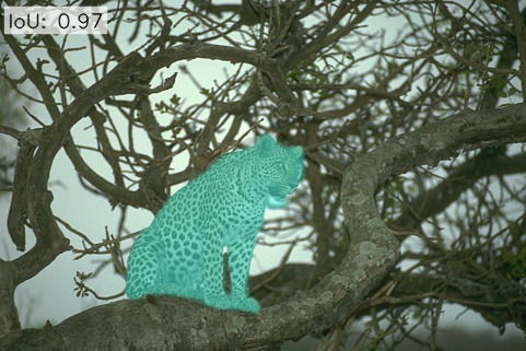
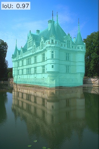
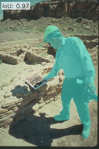
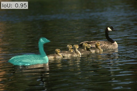
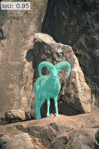
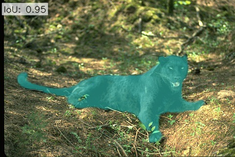
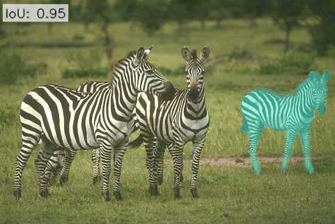
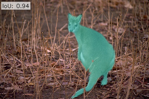
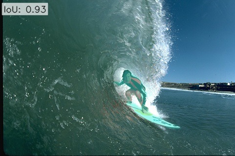
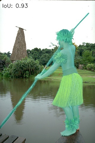
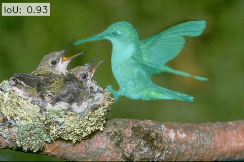
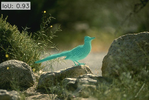
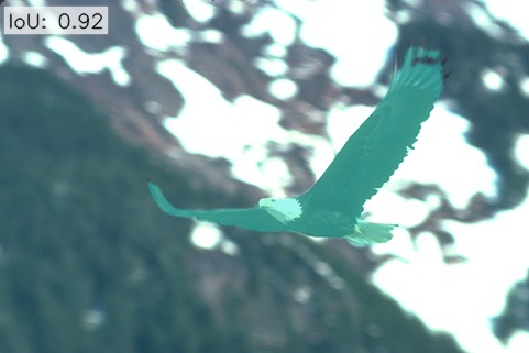
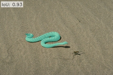
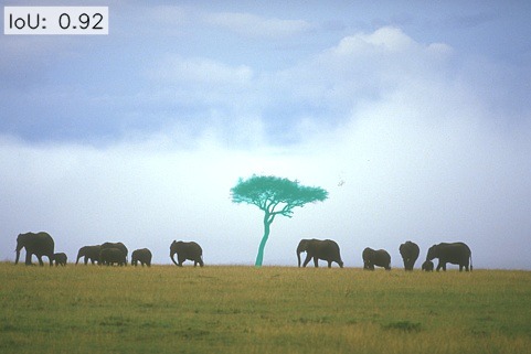
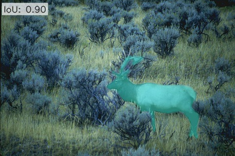
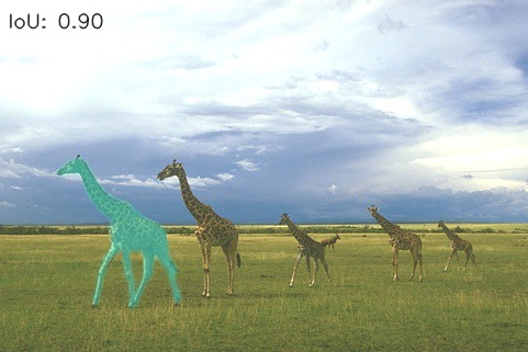
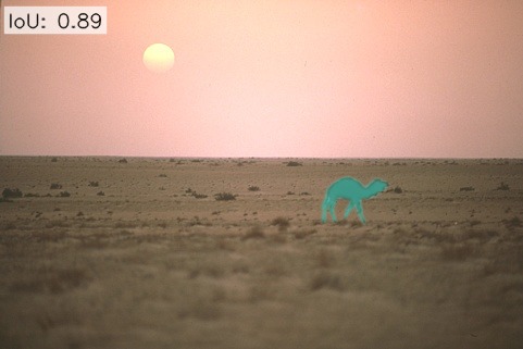
Figure 16: Example predictions from our method at 20 clicks on the Berkeley dataset. Examples are ordered from the easiest (top) to the most difficult images (bottom), based on the mean IoU accuracy over the 15-20 click range. Positive clicks are in red, negative in blue, object masks are highlighted in cyan.

5 Training on a Synthetic Dataset

The two most popular training sets used in interactive segmentation are PASCAL 2012 [5, 37] and SBD [41]. They contain thousands of images labelled by annotators. However, these datasets are also quite imprecise, which is a problem when training very high-quality segmentation networks. Examples of ground-truth delineations can be found in Figure 17. Interestingly, the GrabCut benchmark defines a band of pixel around the object boundary that is excluded when measuring the accuracy. This is not the case with SBD and PASCAL, for which every pixel is evaluated. This partly explains why state of the art techniques achieve higher levels of accuracy on GrabCut.

We can argue that whatever is drawn by the annotators should be considered as ground truth, and that there is no such thing as an incorrect labelling. After all, interactive segmentation algorithms are meant to assist the user achieve whatever arbitrary delineation they want. However, the labelled masks on these datasets would not be good enough in high-end image or video editing applications. These existing datasets are thus not representative of our final application.

We therefore propose to explore how training our network on an accurate and consistently labelled synthetic dataset would impact our overall performance.

5.1 Synthetic Dataset Construction

We constructed our synthetic training dataset in a similar way to the Deep Image Matting dataset from Xu et al. [42]. We sourced 15,000 images of objects with foreground colours and transparencies from the Internet. As illustrated in Figure 18, the images are synthesised on the fly during training by compositing one of these foreground objects onto a randomly sampled background. The background images come from MS-COCO [41] and ETHZ Synthesizability [43] datasets. The binary masks are obtained by thresholding the alpha matte at 0.5. A few examples of such composite training images are shown in Figure 19.

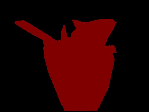
Figure 17: Example of labelling errors in SBD train and validation dataset.

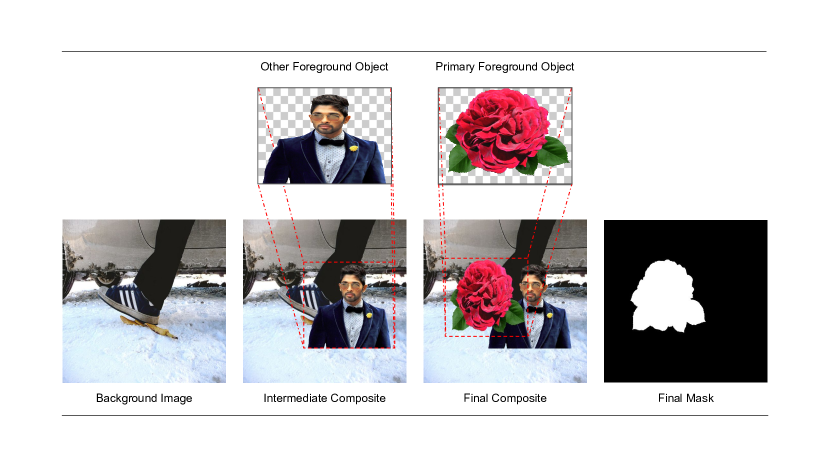
Figure 18: Creating an image of the synthetic dataset.

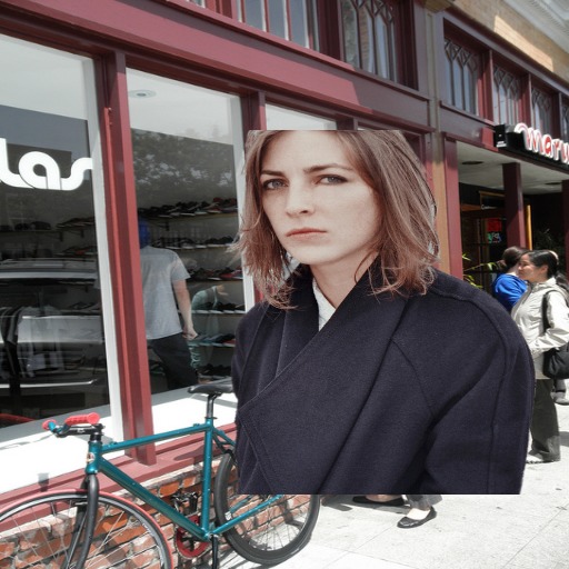
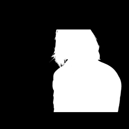
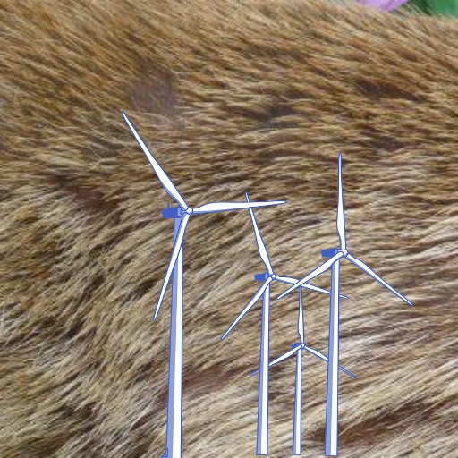
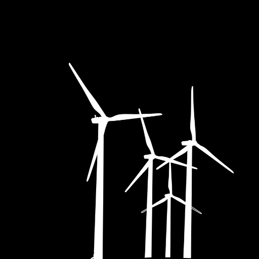
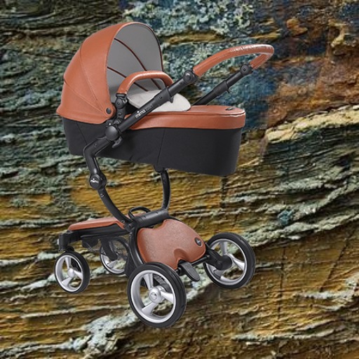
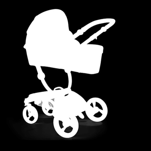
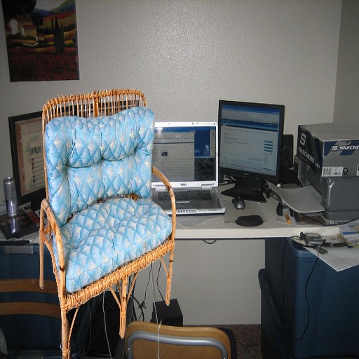
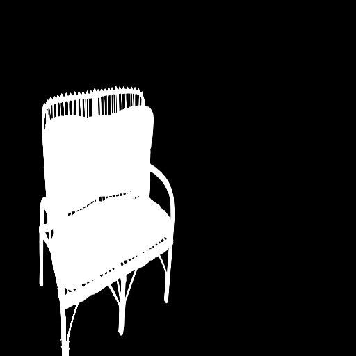
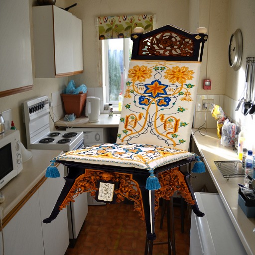
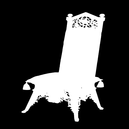
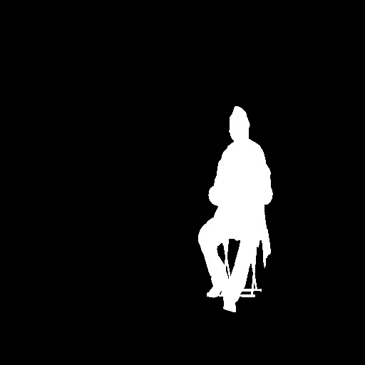
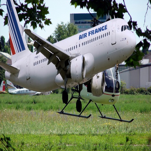
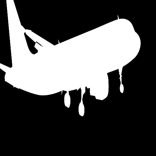
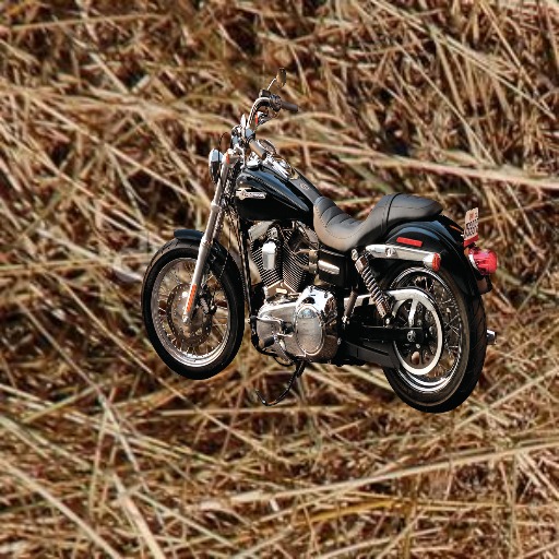
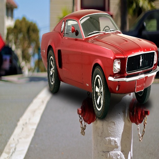
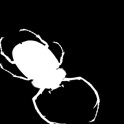
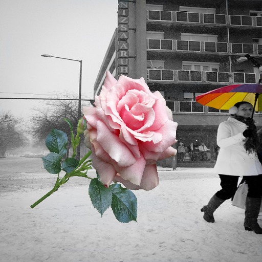
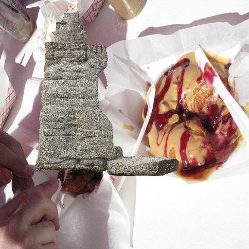
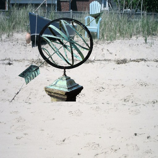
Figure 19: Synthetic Dataset Examples: Variety of training images and their corresponding masks, generated from our Synthetic Dataset.

5.2 Synthetic Dataset Training Results

We propose to analyse the following three training scenarios:

1. our full model (ours:$+T,I,F,G$ ), trained on SBD as proposed in the previous sections

2. our full model (ours:$+T,I,F,G$ w Synth ), solely trained on the synthetic dataset for 10 epochs at fixed learning rate $10^{-5}$.

3. our full model (ours:$+T,I,F,G$ w Synth+FT ), finetuning the previous model on SBD for 5 epochs with learning rate $5\times 10^{-6}$.

The comparisons of the mean IoU over the GrabCut, Berkeley and SBD datasets for these three scenarios is presented in Figures 22, 22 and  22 and examples of the segmentation results at 3 clicks and 20 clicks for the three training approaches are shown in Figure 23 and 24.

Method	GrabCut			Berkeley
	NoC @ 90%	AuC	>99% @ 20 clicks	NoC @ 90%	AuC	>95% @ 20 clicks
ours:$+T,I,F,G$	2.54	0.963	62%	3.53	0.942	81%
ours:$+T,I,F,G$ w Synth	1.96	0.968	74%	3.46	0.943	82%
ours:$+T,I,F,G$ w Synth+FT	1.8	0.974	71%	3.04	0.949	83%

Table 8: Comparison of training with SBD alone(ours:$+T,I,F,G$ ), with the synthetic dataset alone(ours:$+T,I,F,G$ w Synth ), and with finetuning the synthetic model on the SBD set(ours:$+T,I,F,G$ w Synth+FT ). We measure the proportion of images that surpass 95% & 99% accuracy at 20 clicks.

What transpires from these results is that training on the synthetic dataset helps considerably extracting fine details in the masks(see Table 8). This is visible on the examples of Figure 23 and Figure 24. This can also be deduced from the IoU plots on Berkeley and GrabCut, as both synthetic trained (1) and fine tuned (2) versions outperform the SBD trained network (3) as the number of clicks increases.

On the other hand, training on the SBD seems to help with the first few clicks. This makes sense as SBD is designed for rough semantic shapes, whereas our synthetic dataset is not specifically tailored for semantic classes.

We note that the difference between both training sets is most evident on the SBD benchmark, where using the synthetic dataset actually negatively impacts the performance. This makes sense as SBD has only 20 classes, thus training on the SBD training set gives a decisive advantage.

6 Discussion

We have shown that our interactive segmentation method can reach levels of accuracy that can be as high as 99% mIoU. What can be done to achieve higher levels of accuracy? One limitation is that binary segmentation is not well defined for natural images. Pixels at the object boundaries are never either foreground or background but always a mix of both (e.g. hair, fur, motion blur, defocus, etc.). This is exactly what natural matting is trying to solve by defining transparency masks. Thus, instead of interactive segmentation, we should probably aim for interactive matting instead, at least on high-end applications.

One other limitation we observed in this paper is that we are partly limited by the quality of existing training sets. The semantic segmentation datasets available for training and testing are based on real images but are of low quality. On the other hand, the synthetic datasets used in matting, and also in this paper, are of high quality but are not based on real images. There is thus room for much better training sets. The same problem is true for the test sets used in the three popular benchmarks. Going beyond 95% accuracy on the SBD benchmark requires to match a ground truth that does not necessarily follow the actual object boundaries.

In the end, there seems to be two problems in one: rough segmentation and extracting fine details. It is difficult to solve for both in a single unified approach. We can point out to the BRS (Jang and Kim [14]), or FCTSFN (Hu et al. [10]), which split their architectures into two parts: a core network that produces a rough segmentation and, appended to it, a refinement network to upsample the masks. Both networks are trained in stages. In our approach, we show that a single network can be used, but we still resort to a two-stage training when using the synthetic dataset. How to best schedule the training for rough and fine details seems to be key.

	Figure 20: Training with our Synthetic dataset. Mean IoU scores after $n$ clicks for the GrabCut testset [16].
	Figure 21: Training with our Synthetic dataset. Comparison of mean IoU scores after $n$ clicks for the Berkeley testset [15].
	Figure 22: Training with our Synthetic dataset. Comparison of mean IoU scores after $n$ clicks for the SBD testset [37].

Image	Ground Truth	SBD [37]	Synthetic	Synthetic+ SBD

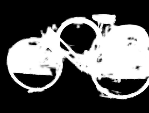
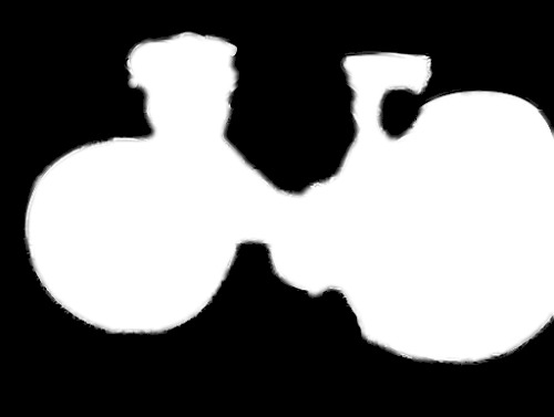
Figure 23: Segmentation examples at 3 clicks, for models trained with SBD, trained with the synthetic dataset alone, and trained with the synthetic set and finetuned on SBD: Images are from the SBD validation set.

Image	Ground Truth	SBD [37]	Synthetic	Synthetic + SBD

Figure 24: Example segmentations at 20 clicks, of models trained with SBD, trained with the synthetic dataset alone, and trained with the synthetic set and finetuned on SBD: Images are from the Berkeley dataset.

7 Conclusion

Existing deep-learning based interactive segmentation methods are of limited use in professional photo editing applications as these methods plateau in accuracy around 95% and yet artists need to achieve more than 99% accuracy. One reason for this plateau is that they insufficiently leverage user interactions. We proposed a novel single network architecture that better embeds the user interactions into two separate streams. Using a click by click training regime helps us improve the correlation between the click placements and the prediction errors. Our experiments show how each contribution improves the response to local corrections and mIoU accuracy across the full range of clicks. In comparison to existing approaches, our method achieves higher accuracy for all 20 measured clicks, across three benchmarks and we even achieve 99% accuracy for 62% of images on the GrabCut dataset within 20 clicks.

We also make the observation that the low quality of existing training sets limits the potential performance of current interactive networks. We show that introducing a more accurate synthetic training set can further improve the overall accuracy of our system, this model reaches 99% accuracy for 74% of images on the GrabCut dataset within 20 clicks.

References

- Boykov and Jolly [2001] Y. Boykov, M.-P. Jolly, Interactive graph cuts for optimal boundary and region segmentation of objects in n-d images, in: Proceedings of the International Conference on Computer Vision, volume 1, 2001, pp. 105–112 vol.1. doi:doi:10.1109/ICCV.2001.937505.
- Kass et al. [1988] M. Kass, A. Witkin, D. Terzopoulos, Snakes: Active contour models, International Journal of Computer Vision 1 (1988) 321–331. doi:doi:10.1007/BF00133570.
- Mortensen and Barrett [1995] E. N. Mortensen, W. A. Barrett, Intelligent scissors for image composition, in: Proceedings of the 22Nd Annual Conference on Computer Graphics and Interactive Techniques, Proceedings of the ACM SIGGRAPH Conference on Computer Graphics, ACM, New York, NY, USA, 1995, pp. 191–198. doi:doi:10.1145/218380.218442.
- Liu et al. [2009] J. Liu, J. Sun, H. Shum, Paint selection, ACM Transactions on Graphics (TOG) 28 (2009) 69. doi:doi:10.1145/1531326.1531375.
- Everingham et al. [2012] M. Everingham, L. Van Gool, C. K. I. Williams, J. Winn, A. Zisserman, The PASCAL Visual Object Classes Challenge 2012 (VOC2012) Results, http://www.pascal-network.org/challenges/VOC/voc2012/workshop/index.html, 2012.
- Xu et al. [2016] N. Xu, B. L. Price, S. Cohen, J. Yang, T. S. Huang, Deep interactive object selection, in: Proceedings of the IEEE Conference on Computer Vision and Pattern Recognition, 2016, pp. 373–381. doi:doi:10.1109/CVPR.2016.47.
- Mahadevan et al. [2018] S. Mahadevan, P. Voigtlaender, B. Leibe, Iteratively trained interactive segmentation, in: British Machine Vision Conference, BMVC, 2018, p. 212.
- Maninis et al. [2018] K. Maninis, S. Caelles, J. Pont-Tuset, L. V. Gool, Deep extreme cut: From extreme points to object segmentation, in: Proceedings of the IEEE Conference on Computer Vision and Pattern Recognition, 2018, pp. 616–625. doi:doi:10.1109/CVPR.2018.00071.
- Bénard and Gygli [2017] A. Bénard, M. Gygli, Interactive Video Object Segmentation in the Wild, Technical Report, gifs.com, 2017.
- Hu et al. [2019] Y. Hu, A. Soltoggio, R. Lock, S. Carter, A fully convolutional two-stream fusion network for interactive image segmentation, Neural Networks 109 (2019) 31–42. doi:doi:10.1016/j.neunet.2018.10.009.
- Li et al. [2018] Z. Li, Q. Chen, V. Koltun, Interactive image segmentation with latent diversity, in: Proceedings of the IEEE Conference on Computer Vision and Pattern Recognition, 2018, pp. 577–585. doi:doi:10.1109/CVPR.2018.00067.
- Majumder and Yao [2019] S. Majumder, A. Yao, Content-aware multi-level guidance for interactive instance segmentation, in: Proceedings of the IEEE Conference on Computer Vision and Pattern Recognition, 2019, pp. 11602–11611.
- Liew et al. [2017] J. Liew, Y. Wei, W. Xiong, S. H. Ong, J. Feng, Regional interactive image segmentation networks, in: Proceedings of the International Conference on Computer Vision, 2017, pp. 2746–2754. doi:doi:10.1109/ICCV.2017.297.
- Jang and Kim [2019] W.-D. Jang, C.-S. Kim, Interactive image segmentation via backpropagating refinement scheme, in: Proceedings of the IEEE Conference on Computer Vision and Pattern Recognition, 2019.
- McGuinness and O’Connor [2010] K. McGuinness, N. E. O’Connor, A comparative evaluation of interactive segmentation algorithms, Pattern Recognition 43 (2010) 434–444. doi:doi:10.1016/j.patcog.2009.03.008.
- Lempitsky et al. [2009] V. S. Lempitsky, P. Kohli, C. Rother, T. Sharp, Image segmentation with a bounding box prior, in: Proceedings of the International Conference on Computer Vision, 2009, pp. 277–284. doi:doi:10.1109/ICCV.2009.5459262.
- Shelhamer et al. [2017] E. Shelhamer, J. Long, T. Darrell, Fully convolutional networks for semantic segmentation, IEEE Transactions on Pattern Analysis and Machine Intelligence 39 (2017) 640–651. doi:doi:10.1109/TPAMI.2016.2572683.
- Bredell et al. [2018] G. Bredell, C. Tanner, E. Konukoglu, Iterative interaction training for segmentation editing networks, in: Machine Learning in Medical Imaging - 9th International Workshop, MLMI 2018, Held in Conjunction with MICCAI 2018, Granada, Spain, September 16, 2018, Proceedings, 2018, pp. 363–370. doi:doi:10.1007/978-3-030-00919-9_42.
- Wu et al. [2018] H. Wu, S. Zheng, J. Zhang, K. Huang, Fast end-to-end trainable guided filter, in: Proceedings of the IEEE Conference on Computer Vision and Pattern Recognition, 2018, pp. 1838–1847. doi:doi:10.1109/CVPR.2018.00197.
- Chen et al. [2016] L.-C. Chen, G. Papandreou, I. Kokkinos, K. Murphy, A. L. Yuille, Deeplab: Semantic image segmentation with deep convolutional nets, atrous convolution, and fully connected crfs., CoRR abs/1606.00915 (2016).
- Ronneberger et al. [2015] O. Ronneberger, P. Fischer, T. Brox, U-net: Convolutional networks for biomedical image segmentation, in: Medical Image Computing and Computer-Assisted Intervention - MICCAI, 2015, pp. 234–241. doi:doi:10.1007/978-3-319-24574-4_28.
- Deng et al. [2009] J. Deng, W. Dong, R. Socher, L.-J. Li, K. Li, L. Fei-Fei, ImageNet: A Large-Scale Hierarchical Image Database, in: Proceedings of the IEEE Conference on Computer Vision and Pattern Recognition, 2009.
- Simonyan and Zisserman [2014] K. Simonyan, A. Zisserman, Very deep convolutional networks for large-scale image recognition, CoRR abs/1409.1556 (2014).
- Chollet [2017] F. Chollet, Xception: Deep learning with depthwise separable convolutions, in: Proceedings of the IEEE conference on computer vision and pattern recognition, 2017, pp. 1251–1258.
- Chen et al. [2018] L.-C. Chen, Y. Zhu, G. Papandreou, F. Schroff, H. Adam, Encoder-decoder with atrous separable convolution for semantic image segmentation, in: Proceedings of the European conference on computer vision (ECCV), 2018, pp. 801–818.
- He et al. [2016] K. He, X. Zhang, S. Ren, J. Sun, Deep residual learning for image recognition, in: Proceedings of the IEEE conference on computer vision and pattern recognition, 2016, pp. 770–778.
- Chen et al. [2017] L.-C. Chen, G. Papandreou, I. Kokkinos, K. Murphy, A. L. Yuille, Deeplab: Semantic image segmentation with deep convolutional nets, atrous convolution, and fully connected crfs, IEEE transactions on pattern analysis and machine intelligence 40 (2017) 834–848.
- Krähenbühl and Koltun [2011] P. Krähenbühl, V. Koltun, Efficient inference in fully connected crfs with gaussian edge potentials, in: Advances in neural information processing systems, 2011, pp. 109–117.
- Chen et al. [2017] Q. Chen, J. Xu, V. Koltun, Fast image processing with fully-convolutional networks, in: Proceedings of the IEEE International Conference on Computer Vision, 2017, pp. 2497–2506.
- Huang et al. [2017] G. Huang, Z. Liu, L. Van Der Maaten, K. Q. Weinberger, Densely connected convolutional networks, in: Proceedings of the IEEE conference on computer vision and pattern recognition, 2017, pp. 4700–4708.
- Wu and He [2018] Y. Wu, K. He, Group normalization, in: Proceedings of the European Conference on Computer Vision, 2018, pp. 3–19. doi:doi:10.1007/978-3-030-01261-8_1.
- Qiao et al. [2019] S. Qiao, H. Wang, C. Liu, W. Shen, A. Yuille, Weight standardization, arXiv preprint arXiv:1903.10520 (2019).
- Zhao et al. [2017] H. Zhao, J. Shi, X. Qi, X. Wang, J. Jia, Pyramid scene parsing network, in: Proceedings of the IEEE Conference on Computer Vision and Pattern Recognition, 2017, pp. 6230–6239. doi:doi:10.1109/CVPR.2017.660.
- Wu et al. [2018] H. Wu, S. Zheng, J. Zhang, K. Huang, Fast end-to-end trainable guided filter, in: Proceedings of the IEEE Conference on Computer Vision and Pattern Recognition, 2018.
- Le et al. [2018] H. Le, L. Mai, B. L. Price, S. Cohen, H. Jin, F. Liu, Interactive boundary prediction for object selection, in: Proceedings of the European Conference on Computer Vision, 2018, pp. 20–36. doi:doi:10.1007/978-3-030-01264-9_2.
- Nicholas Bloch [2015] A. M. Nicholas Bloch, Nci-isbi 2013 challenge: Automated segmentation of prostate structures, 2015. doi:doi:10.7937/K9/TCIA.2015.ZF0VLOPV.
- Hariharan et al. [2011] B. Hariharan, P. Arbelaez, L. D. Bourdev, S. Maji, J. Malik, Semantic contours from inverse detectors, in: Proceedings of the International Conference on Computer Vision, 2011, pp. 991–998. doi:doi:10.1109/ICCV.2011.6126343.
- Maas et al. [2013] A. L. Maas, A. Y. Hannun, A. Y. Ng, Rectifier nonlinearities improve neural network acoustic models, Proc. ICML (2013).
- Nickisch et al. [2010] H. Nickisch, C. Rother, P. Kohli, C. Rhemann, Learning an interactive segmentation system, in: ICVGIP, 2010, pp. 274–281. doi:doi:10.1145/1924559.1924596.
- Liu et al. [2019] L. Liu, H. Jiang, P. He, W. Chen, X. Liu, J. Gao, J. Han, On the variance of the adaptive learning rate and beyond, 2019. arXiv:1908.03265.
- Lin et al. [2014] T. Lin, M. Maire, S. J. Belongie, J. Hays, P. Perona, D. Ramanan, P. Dollár, C. L. Zitnick, Microsoft COCO: common objects in context, in: Proceedings of the European Conference on Computer Vision, 2014, pp. 740–755. doi:doi:10.1007/978-3-319-10602-1_48.
- Xu et al. [2017] N. Xu, B. Price, S. Cohen, T. Huang, Deep image matting, in: Proceedings of the IEEE Conference on Computer Vision and Pattern Recognition, 2017.
- Dai et al. [2014] D. Dai, H. Riemenschneider, L. V. Gool, The synthesizability of texture examples, in: Proceedings of the IEEE Conference on Computer Vision and Pattern Recognition, 2014, pp. 3027–3034. doi:doi:10.1109/CVPR.2014.387.