Rotational excitations in rare-earth nuclei: a comparative study within three cranking models with different mean fields and the treatments of pairing correlations

Abstract

High-spin rotational bands in rare-earth Er ($Z=68$), Tm ($Z=69$) and Yb ($Z=70$) isotopes are investigated by three different nuclear models. These are (i) the cranked relativistic Hartree-Bogoliubov (CRHB) approach with approximate particle number projection by means of the Lipkin-Nogami (LN) method, (ii) the cranking covariant density functional theory (CDFT) with pairing correlations treated by a shell-model-like approach (SLAP) or the so called particle-number conserving (PNC) method, and (iii) cranked shell model (CSM) based on the Nilsson potential with pairing correlations treated by the PNC method. A detailed comparison between these three models in the description of the ground state rotational bands of even-even Er and Yb isotopes is performed. The similarities and differences between these models in the description of the moments of inertia, the features of band crossings, equilibrium deformations and pairing energies of even-even nuclei under study are discussed. These quantities are considered as a function of rotational frequency and proton and neutron numbers. The changes in the properties of the first band crossings with increasing neutron number in this mass region are investigated. On average, a comparable accuracy of the description of available experimental data is achieved in these models. However, the differences between model predictions become larger above the first band crossings. Because of time-consuming nature of numerical calculations in the CDFT-based models, a systematic study of the rotational properties of both ground state and excited state bands in odd-mass Tm nuclei is carried out only by the PNC-SCM. With few exceptions, the rotational properties of experimental 1-quasiparticle and 3-quasiparticle bands in ^{165,167,169,171}Tm are reproduced reasonably well. The appearance of backbendings or upbendings in these nuclei is well understood from the analysis of the variations of the occupation probabilities of the single-particle states and their contributions to total angular momentum alignment with rotational frequency.

I Introduction

The increase of angular momentum towards extreme values triggers the appearance of different physical phenomena such as backbending Johnson et al. (1971); Lee et al. (1977), band termination Bengtsson and Ragnarsson (1983); Afanasjev et al. (1999a), signature inversion Bengtsson et al. (1984), superdeformation Twin et al. (1986), wobbling motion Ødegård et al. (2001), etc. The rare-earth nuclei with $N\sim 100$ and $A\sim 170$ are particularly rich in such phenomena. In this mass region, the nuclei have prolate shapes at ground states but the yrast and near-yrast structures at medium and high spin are built by a significant number of multi-quasiparticle (qp) configurations with different degree of triaxiality. In even-even nuclei the transition from ground state rotational band to 2-qp band is triggered by first paired band crossing leading either to backbending or upbending. The backbending has first been observed in ¹⁶⁰Dy ($Z=66$) in the pioneering work of Ref. Johnson et al. (1971), and later it was interpreted as the alignment of one pair of the $i_{13/2}$ neutrons Stephens and Simon (1972). Thus, the determination of the nature of band crossings allows to identify involved single-particle states and quasiparticle configurations along the yrast line (see Refs. de Voigt et al. (1983); Szymański (1983)).

As compared with even-even nuclei, the odd-$A$ systems at low to medium spins provide much richer experimental data and thus give deeper insight into single-particle and shell structures in the vicinity of the Fermi level. This can be illustrated by the Tm $(Z=69)$ isotopes which are used in the present manuscript as a testing ground for different theoretical approaches. For example, the ground state bands (GSB) in the $N=96-102$ Tm isotopes are build on the $\pi 1/2^{+}[411]$ Nilsson state. Recently, the experimental evidence of a sharp backbending in this band has been observed in the ¹⁶⁹Tm nucleus Asgar et al. (2017). The backbending is also sharp in this band in ¹⁶⁵Tm Jensen et al. (2001). On the contrary, the situation is completely different in the ¹⁶⁷Tm nucleus (which is located between two above mentioned nuclei) the GSB of which shows only a smooth upbending  Burns et al. (2005). These features could provide a detailed information on the single-particle level distribution in the vicinity of the Fermi level and yrast-yrare interaction Bengtsson et al. (1978); Wu and Zeng (1991a).

Over the years the experimental data on rotating rare-earth nuclei have been used as a testing ground for various theoretical models such as the cranked Nilsson-Strutinsky method Andersson et al. (1976), the cranked shell model (CSM) with Nilsson Bengtsson and Frauendorf (1979) and Woods-Saxon Nazarewicz et al. (1985); Ćwiok et al. (1987) potentials, the projected shell model Hara and Sun (1995), the tilted axis cranking model Frauendorf (2001), the cranked relativistic (covariant) Afanasjev et al. (1996, 2000a) and non-relativistic density functional theories (DFTs) Terasaki et al. (1995); Egido and Robledo (1993); Afanasjev et al. (2000a), etc. They differ by employed assumptions and approximations and range from simple CSM based on phenomenological potentials to much more microscopic cranked DFTs. In the present manuscript, the experimental data on the $N=96-102$ Er $(Z=68)$, Tm $(Z=69)$ and Yb $(Z=70$) nuclei will be used for a comparative analysis of three different theoretical approaches, namely,

1. The cranked relativistic Hartree-Bogoliubov approach with pairing correlations treated by approximate particle number projection by means of the Lipkin-Nogami method (further abbreviated as CRHB+LN Afanasjev et al. (2000b)).

2. The cranking covariant density functional theory with pairing correlations treated by the shell-model-like approach (further abbreviated as cranking CDFT-SLAP Shi et al. (2018)).

3. The particle-number conserving method based on the cranked shell model in which the phenomenological Nilsson potential is adopted for the mean field (further abbreviated as PNC-CSM Zeng et al. (1994a)).

The first two methods are based on covariant density functional theory (CDFT), while the latter one on phenomenological Nilsson potential. The latter two approaches use the same particle-number conserving method, while the first one is based on approximate particle number projection by means of the Lipkin-Nogami (LN) method. The goals of this study are (i) to evaluate the weak and strong points of these approaches, (ii) to estimate to which extent approximate particle number projection by means of the LN method is a good approximation to the particle-number conserving method, and (iii) to evaluate typical accuracy of the description of experimental data by these methods.

CDFT Ring (1996); Vretenar et al. (2005); Meng et al. (2006a) is well suited for the description of rotational structures. It exploits basic properties of QCD at low energies, in particular, the symmetries and the separation of scales Lal (2004). Built on the Dirac equation, it provides a consistent treatment of the spin degrees of freedom Lal (2004); Cohen et al. (1992) and spin-orbit splittings Bender et al. (1999); Litvinova and Afanasjev (2011). The latter has significant influence on the shell structure. It also includes the complicated interplay between the large Lorentz scalar and vector self-energies induced on the QCD level by the in-medium changes of the scalar and vector quark condensates Cohen et al. (1992). Lorentz covariance of CDFT leads to the fact that time-odd mean fields of this theory are determined as spatial components of Lorentz vectors and therefore coupled with the same constants as the time-like components Afanasjev and Abusara (2010a), which are fitted to ground-state properties of finite nuclei. This is extremely important for the description of nuclear rotations Afanasjev and Ring (2000); Vretenar et al. (2005); Meng et al. (2013). Using cranked versions of CDFT, many rotational phenomena such as superdeformation at high spin König and Ring (1993); Afanasjev et al. (1996, 2000b), smooth band termination Vretenar et al. (2005), magnetic Madokoro et al. (2000); Peng et al. (2008); Zhao et al. (2011a, 2015a) and antimagnetic Zhao et al. (2011b, 2012); Liu (2019) rotations, nuclear chirality Zhao (2017), clusterization at high spins Zhao et al. (2015b); Zhao and Li (2018); Afanasjev and Abusara (2018); Ren et al. (2019), the birth and death of particle-bound rotational bands and the extension of nuclear landscape beyond spin zero neutron drip line Afanasjev et al. (2019) have been investigated successfully.

The Nilsson potential Nilsson (1955); Nilsson et al. (1969); Nilsson and Ragnarsson (1995) has been used in the calculations of rotational properties for more that half of century. Contrary to the CDFT, cranking approaches based on this potential lack full self-consistency and do not include time-odd mean fields. Despite that they are still quite powerful theoretical tools which have high predictive power. They have been instrumental in the prediction of superdeformation and smooth band termination at high spin as well as magnetic, antimagnetic and chiral rotations (see Refs. Nilsson and Ragnarsson (1995); Afanasjev et al. (1999a); Frauendorf (2001) and references quoted therein). They are still extensively used by Lund and Notre-Dame groups in the interpretation of recent experimental data Petrache et al. (2019); Bhattacharya et al. (2019). This is in part due to the fact that cranking approaches based on the Nilsson potential are by the orders of magnitude numerically less time consuming that those based on the DFT approaches.

Pairing correlations are extremely important for the description of rotational properties such as the moment of inertia (MOI), the frequencies of paired band crossings leading either to backbendings or upbendings, the alignment gains at paired band crossings, etc Bohr and Mottelson (1975); Ring and Schuck (1980); Meng (2015). They are usually treated by the Bardeen-Cooper-Schrieffer (BCS) or Hartree-Fock-Bogoliubov (HFB) approaches within the mean-field approximation Ring and Schuck (1980). However, in these two standard methods pairing collapse takes place either at a critical rotational frequency $\omega_{\rm c}$ Mottelson and Valatin (1960) or a critical temperature $T_{\rm c}$ Sano and Wakai (1972). To restore this broken symmetry, a number of approximate methods of particle number restoration have been developed in the past. One of most widely used is the Lipkin-Nogami method Lipkin (1960, 1961); Nogami (1964), which considers the second-order correction of the particle-number fluctuation. When this method is implemented, the pairing collapse does not appear in the solutions of the cranked HFB equations for a substantially large frequency range Gall et al. (1994); Valor et al. (1996); Afanasjev et al. (2000b). In particular, the CRHB+LN calculations successfully describe experimental data on rotational properties across the nuclear chart and different physical phenomena such as the rotation of normal deformed nuclei, super- and hyperdeformation at high spin, pairing phase transition, role of proton-neutron pairing in $N\approx Z$ nuclei, etc Afanasjev et al. (1999b, 2000b); O’Leary et al. (2003); Afanasjev and Abdurazakov (2013); Afanasjev (2014); Jeppesen et al. (2009); Herzberg et al. (2009); Afanasjev and Frauendorf (2005); Ray and Afanasjev (2016); Andreoiu et al. (2007); Davies et al. (2007). However, the investigations have shown that the LN method breaks down in the weak pairing limit Dobaczewski and Nazarewicz (1993); Sheikh et al. (2002) leading to pairing collapse. This is especially a case for extremely high rotational frequencies and for rotational bands built on multi-qp pair-broken excited configurations. It turns out that for such situations the calculations without pairing provide quite accurate description of experimental rotational properties Afanasjev et al. (1996, 1999a); Afanasjev and Frauendorf (2005).

In addition, various particle-number projection approaches based on the BCS or HFB formalism have been developed over the time Ring and Schuck (1980); Egido and Ring (1982); Anguiano et al. (2001); Volya et al. (2001); Stoitsov et al. (2007); Bender et al. (2009); Yao et al. (2014). In these approaches, the ideal treatment is the variation after projection. However, such methods are very complicated and computationally extremely expensive for deformed rotational structures. To overcome these problems, alternative non-variational methods aiming at the diagonalization of the many-body Hamiltonian directly have been developed Zeng and Cheng (1983); Pillet et al. (2002). In this so-called shell-model-like approach (SLAP) Meng et al. (2006b), or originally referred as particle-number conserving (PNC) method Zeng and Cheng (1983), the pairing Hamiltonian is diagonalized directly in a properly truncated Fock-space Wu and Zeng (1989). In the SLAP/PNC approach, both particle number conservation and the Pauli blocking effects are treated exactly. Note that the SLAP/PNC method has been built into theoretical approaches based on CSM with the Nilsson Zeng et al. (1994a) and Woods-Saxon Molique and Dudek (1997); Fu et al. (2013) potentials as well as on those based on relativistic Meng et al. (2006b) and non-relativistic Liang et al. (2015) DFTs. These methods have been successful in the description of different nuclear phenomena in rotating nuclei such as odd-even differences in MOI Zeng et al. (1994b), identical bands Zeng et al. (2001); Liu et al. (2002), nuclear pairing phase transition Wu et al. (2011), antimagnetic rotation Zhang et al. (2013a); Zhang (2016); Liu (2019); Zhang (2019), and high-$K$ rotational bands in the rare-earth nuclei Zhang et al. (2009); Zhang (2018); He and Li (2018); Liu et al. (2019); Dai and Xu (2019), and rotational bands in actinides He et al. (2009); Zhang et al. (2011, 2012, 2013b); Fu et al. (2014). Note that similar approaches to treat pairing correlations with exactly conserved particle number can be found in Refs. Richardson and Sherman (1964); Pan et al. (1998); Volya et al. (2001); Jia (2013a, b); Chen et al. (2014).

The paper is organized as follows. Theoretical frameworks of the CRHB+LN, cranking CDFT-SLAP and PNC-CSM approaches are presented in Sec. II. The structure of point-coupling and meson-exchange covariant energy density functionals (CEDFs) and of the Nilsson potential is considered in this section too. Two methods for the treatment of pairing, i.e., the SLAP (or PNC) and LN, are also discussed. The numerical details of the present calculations are given in Sec. III. The results of the calculations for even-even Er and Yb isotopes obtained within these three approaches as well as a detailed comparison of these results are reported in Sec. IV. The results for odd-proton Tm nuclei are presented in Sec. V; because of numerical limitations the major focus is on the excitation energies and MOIs of the 1- and 3-qp configurations obtained in the PNC-CSM calculations. In addition, the evolution of backbendings/upbendings with increasing neutron number is discussed. Finally, Sec. VI summarizes the results of our work.

II Theoretical framework

In this section we will give a brief introduction to the cranked CDFT and CSM approaches and the methods for treating the pairing correlations, namely, SLAP and the LN method. Note that the cranking methods discussed are based on one-dimensional cranking approximation.

II.1 The shell-model-like approach

The cranking many-body Hamiltonian with pairing correlations can be written as

$$\hat{H}=\hat{H}_{0}+\hat{H}_{\rm P}.$$ (1)

Here the one-body Hamiltonian is given by

$$\hat{H}_{0}=\sum\hat{h}_{0}=\sum(h_{\rm s.p.}-\omega_{x}j_{x}),$$ (2)

and $\hat{H}_{\rm P}$ is pairing Hamiltonian. $h_{\rm s.p.}$ and $-\omega_{x}j_{x}$ are the single-particle Hamiltonian and Coriolis term, respectively. $h_{\rm s.p.}$ can be represented by any mean field Hamiltonian. So far the SLAPs based on phenomenological Nilsson Zeng et al. (1994a) and Woods-Saxon Fu et al. (2013) potentials and non-relativistic (Skyrme Hartree-Fock approach Liang et al. (2015)) and relativistic (CDFT Shi et al. (2018)) DFTs have been developed. In the present work, we employ two SLAPs: one is based on microscopic cranked CDFT approach and another on phenomenological cranked Nilsson Hamiltonian.

The basic idea of SLAP is to diagonalize the many-body Hamiltonian (1) directly in a sufficiently large many-particle configuration (MPC) space, characterized by an exact particle number Zeng and Cheng (1983), which is constructed from the cranked single-particle states. After diagonalizing the one-body Hamiltonian $\hat{H}_{0}$, one can obtain the single-particle routhians $\varepsilon_{\mu\alpha}$

$$\hat{H}_{0}=\sum_{\mu\alpha}\varepsilon_{\mu\alpha}\hat{b}^{\dagger}_{\mu\alpha}\hat{b}_{\mu\alpha},$$ (3)

and the corresponding eigenstate $|\mu\alpha\rangle$ (denoted further by $|\mu\rangle$)

$$|\mu\alpha\rangle=\sum_{\xi}C_{\mu\xi}(\alpha)|\xi\alpha\rangle,$$ (4)

for each level $\mu$ with the signature $\alpha$. Therefore, the MPC $|i\rangle$ for the $n$-particle system can be constructed as Zeng et al. (1994a)

$$|i\rangle=|\mu_{1}\mu_{2}\cdots\mu_{n}\rangle=\hat{b}^{\dagger}_{\mu_{1}}\hat{b}^{\dagger}_{\mu_{2}}\cdots\hat{b}^{\dagger}_{\mu_{n}}|0\rangle.$$ (5)

The parity $\pi$, signature $\alpha$, and the corresponding configuration energy for each MPC are obtained from the occupied single-particle states. By diagonalizing the cranking many-body Hamiltonian (1) in a sufficiently large MPC space (a dimension of 1000 for both protons and neutrons is good enough for rare-earth nuclei), reasonably accurate solutions for the ground state and low-lying excited eigenstates can be obtained. Their wavefunctions can be written as

$$|\Psi\rangle=\sum_{i}C_{i}\left|i\right\rangle,\qquad(C_{i}\;\textrm{real}),$$ (6)

where $C_{i}$ are the corresponding expansion coefficients.

For the state $|\Psi\rangle$, the angular momentum alignment is given by

$$\langle\Psi|J_{x}|\Psi\rangle=\sum_{i}C_{i}^{2}\langle i|J_{x}|i\rangle+2\sum_{i<j}C_{i}C_{j}\langle i|J_{x}|j\rangle,$$ (7)

and the kinematic MOI by

$$J^{(1)}=\frac{1}{\omega_{x}}\langle\Psi|J_{x}|\Psi\rangle.$$ (8)

Because $J_{x}$ is a one-body operator, the matrix element $\langle i|J_{x}|j\rangle$ ($i\neq j$) may be non-zero only when the states $|i\rangle$ and $|j\rangle$ differ by one particle occupation Zeng et al. (1994a). After a certain permutation of creation operators, $|i\rangle$ and $|j\rangle$ can be recast into

$$|i\rangle=(-1)^{M_{i\mu}}|\mu\cdots\rangle,\qquad|j\rangle=(-1)^{M_{j\nu}}|\nu\cdots\rangle,$$ (9)

where $\mu$ and $\nu$ denote two different single-particle states, and $(-1)^{M_{i\mu}}=\pm 1$, $(-1)^{M_{j\nu}}=\pm 1$ depend on whether the permutation is even or odd. Therefore, the angular momentum alignment of $|\Psi\rangle$ can be expressed as

$$\langle\Psi|J_{x}|\Psi\rangle=\sum_{\mu}j_{x}(\mu)+\sum_{\mu<\nu}j_{x}(\mu\nu),$$ (10)

where the diagonal term $j_{x}(\mu)$ and the off-diagonal (interference) term $j_{x}(\mu\nu)$ can be written as

$$j_{x}(\mu) = \langle\mu|j_{x}|\mu\rangle n_{\mu},$$ (11)

$$j_{x}(\mu\nu) = 2\langle\mu|j_{x}|\nu\rangle\sum_{i<j}(-1)^{M_{i\mu}+M_{j\nu}}C_{i}C_{j}\quad(\mu\neq\nu).$$

The occupation probability $n_{\mu}$ of cranked single-particle orbital $|\mu\rangle$ is given by

$$n_{\mu}=\sum_{i}|C_{i}|^{2}P_{i\mu}.$$ (13)

$P_{i\mu}=1$ if $|\mu\rangle$ is occupied in MPC $|i\rangle$, and $P_{i\mu}=0$ otherwise. Note that in the cranking CDFT-SLAP, the occupation probabilities will be iterated back into the densities and currents in Table 2 to achieve self-consistency Meng et al. (2006b); Shi et al. (2018).

In general, the pairing Hamiltonian $\hat{H}_{\rm P}$ can be written as

$$\hat{H}_{\rm P}=\hat{H}_{\rm pair-mon}+\hat{H}_{\rm pair-quad}+O({\rm higher\,\,order}),$$ (14)

with

$$\hat{H}_{\rm pair-mon} = -G_{0}\sum_{\xi,\eta>0}^{\xi\neq\eta}\hat{\beta}^{\dagger}_{\xi}\hat{\beta}^{\dagger}_{\bar{\xi}}\hat{\beta}_{\bar{\eta}}\hat{\beta}_{\eta},$$ (15)

$$H_{\rm pair-quad} = -G_{2}\sum_{\xi\eta}q_{2}(\xi)q_{2}(\eta)\hat{\beta}^{\dagger}_{\xi}\hat{\beta}^{\dagger}_{\bar{\xi}}\hat{\beta}_{\bar{\eta}}\hat{\beta}_{\eta},$$ (16)

being the Hamiltonians of monopole and quadrupole pairing and $G_{0}$ and $G_{2}$ their effective pairing strengths. Higher order terms are usually neglected. Note that $\bar{\xi}$ ($\bar{\eta}$) labels the time-reversal state of $\xi$ ($\eta$), and $\xi\neq\eta$ means that the self-scattering of the nucleon pairs is forbidden Meng et al. (2006b). In Eq. (16), $q_{2}(\xi)$ and $q_{2}(\eta)$ are the diagonal elements of the stretched quadrupole operator. It turns out that reasonable agreement with experiment is obtained in cranking CDFT-SLAP with only monopole pairing Shi et al. (2018); recent investigation of Ref. Xiong (2019) has shown that with renormalized pairing strengths the cranking CDFT-SLAP results with monopole pairing are quite similar to those obtained with the separable pairing force of Ref. Tian et al. (2009). Thus, we only include monopole pairing in the cranking CDFT-SLAP code. On the contrary, the addition of quadrupole pairing is necessary in the SLAP with Nilsson potential.

In the SLAP, the pairing energy $E_{\rm pair}$ due to pairing correlations is defined as

$$E_{\rm pair}=\langle\Psi|\hat{H}_{\rm P}|\Psi\rangle.$$ (17)

II.2 Cranked relativistic Hartree-Bogliuobov approach with approximate particle number projections by means of Lipkin-Nogami method

The cranked relativistic Hartree-Bogoluibov (CRHB) equations with approximate particle number projection by means of the Lipkin-Nogami (LN) method (further CRHB+LN) are given by Afanasjev et al. (1999b, 2000b)

$$\left(\begin{array}[]{cc}\hat{h}_{\rm D}\left(\eta\right)-\lambda\left(\eta\right)-\omega_{x}\hat{J}_{x}&\hat{\Delta}\left(\eta\right)\\ -\hat{\Delta}^{\ast}\left(\eta\right)&-\hat{h}_{\rm D}^{\ast}\left(\eta\right)+\lambda\left(\eta\right)+\omega_{x}\hat{J}_{x}^{\ast}\end{array}\right)\left(\begin{array}[]{c}U\left(\bm{r}\right)\\ V\left(\bm{r}\right)\end{array}\right)_{k}=E_{k}\left(\eta\right)\left(\begin{array}[]{c}U\left(\bm{r}\right)\\ V\left(\bm{r}\right)\end{array}\right)_{k},$$ (18)

where

$$\hat{h}_{\rm D}(\eta) = \hat{h}_{\rm D}+2\lambda_{2}\,[(1+\eta)\rho-{\rm Tr}(\rho)],$$ (19)

$$\hat{\Delta}(\eta) = \hat{\Delta}-2\lambda_{2}(1-\eta)\kappa,$$ (20)

$$\lambda(\eta) = \lambda_{1}+\lambda_{2}\,[1+\eta],$$ (21)

$$E_{k}(\eta) = E_{k}-\eta\lambda_{2}.$$ (22)

Here $\hat{h}_{\rm D}$ is the single-nucleon Dirac Hamiltonian the structure of which is discussed in more detail in Sec. II.3. $\hat{\Delta}$ is the pairing potential, $U_{k}$ and $V_{k}$ are quasiparticle Dirac spinors and $E_{k}$ denote the quasiparticle energies.

The $\lambda_{2}$ value used in the CRHB+LN calculations is given by

$$\lambda_{2}=-\frac{1}{4}\frac{{\rm Tr}_{2}{\rm Tr}_{2}(\kappa^{\ast}\rho\,\overline{v}\,\sigma\kappa)}{[{\rm Tr}(\kappa\kappa^{\dagger})]^{2}-2{\rm Tr}(\kappa\kappa^{\dagger}\kappa\kappa^{\dagger})}.$$ (23)

where $\sigma=1-\rho$ and $\overline{v}_{abcd}=\langle ab|V^{pp}|cd-dc\rangle$ is antisymmetrized matrix element of the two-particle interaction $V^{pp}$. The trace ${\rm Tr}_{2}$ represents the summation in the particle-particle channel. Note that the density matrix $\rho$ and pairing tensor $\kappa$ entering into Eq. (23) are real.

The presence of the parameter $\eta\,(\eta=0,\pm 1)$ is the consequence of the fact that the form of the CRHB+LN equations is not unique (see Ref. Afanasjev et al. (2000b) for detail). The application of the LN method leads to a modification of the CRHB equations for the fermions, while the mesonic part of the CRHB theory is not affected. This modification is obtained by the restricted variation of $\lambda_{2}\langle(\Delta N)^{2}\rangle$, namely, $\lambda_{2}$ is not varied and its value is calculated self-consistently using Eq. (23) in each step of the iteration. In the present calculations we are using the case of $\eta=+1$ which provides reasonable numerical stability of the CRHB+LN equations. It corresponds to the shift of whole modification into the particle-hole channel of the CRHB+LN theory: $\hat{h}_{\rm D}\rightarrow\hat{h}_{\rm D}+4\lambda_{2}\rho-2\lambda_{2}{\rm Tr}(\rho)$ leaving pairing potential $\hat{\Delta}$ unchanged.

In the CRHB theory the phenomelogical Gogny-type finite range interaction

$$V^{pp}(1,2)= f\sum_{i=1,2}e^{-[({\bm{r}}_{1}-{\bm{r}}_{2})/\mu_{i}]^{2}}$$ (24)

$$\times(W_{i}+B_{i}P^{\sigma}-H_{i}P^{\tau}-M_{i}P^{\sigma}P^{\tau}),$$

is used in the pairing channel. Here $\mu_{i}$, $W_{i}$, $B_{i}$, $H_{i}$ and $M_{i}$ $(i=1,2)$ are the parameters of the force and $P^{\sigma}$ and $P^{\tau}$ are the exchange operators for the spin and isospin variables, respectively. The parameter set D1S Berger et al. (1991) is employed for the Gogny pairing force. A scaling factor $f$ is used here for fine tuning of pairing properties to the mass region under study Afanasjev and Abdurazakov (2013). A clear advantage of the Gogny pairing force is that all multipoles of the interaction are taken into account in the pairing channel.

The expectation value of the total angular momentum along the rotational axis is given by

$$J={\rm Tr}(j_{x}\rho),$$ (25)

and the size of pairing correlations is measured in terms of the pairing energy

$$E_{\rm pair}=-\frac{1}{2}\rm{Tr}(\Delta\kappa).$$ (26)

This is not an experimentally accessible quantity, but it is a measure for the size of the pairing correlations in theoretical calculations.

II.3 Covariant energy density functionals

The cranking CDFT-SLAP and CRHB+LN calculations are performed with CEDFs representative of two classes of CDFT models Agbemava et al. (2014), namely, (i) those based on meson exchange with non-linear meson couplings (NLME), and (ii) those based on point coupling (PC) models with zero-range interaction terms in the Lagrangian. In NLME models, the exchange of mesons with finite masses leads to finite-range interaction. In PC models, the gradient terms simulate the effects of finite range.

The Lagrangians of these two classes of the functionals can be written as: $\mathcal{L}=\mathcal{L}_{\rm common}+\mathcal{L}_{\rm model-specific}$ where the $\mathcal{L}_{\rm common}$ consists of the Lagrangian of the free nucleons and the electromagnetic interaction. It is identical for all two classes of functionals and is written as

$$\mathcal{L}_{\rm common}=\mathcal{L}^{\rm free}+\mathcal{L}^{\rm em},$$ (27)

with

$$\mathcal{L}^{\rm free}=\bar{\psi}(i\gamma_{{\mu}}\partial^{\mu}-m)\psi,$$ (28)

and

$$\mathcal{L}^{\rm em}=-\frac{1}{4}F^{\mu\nu}F_{\mu\nu}-e\frac{1-\tau_{3}}{2}\bar{\psi}\gamma^{\mu}\psi A_{\mu}.$$ (29)

For each model there is a specific term in the Lagrangian: for the NLME models we have

$$\mathcal{L}_{\rm NLME} = \frac{1}{2}(\partial{\sigma})^{2}-\frac{1}{2}m_{\sigma}^{2}\sigma^{2}-\frac{1}{4}\Omega_{\mu\nu}\Omega^{\mu\nu}+\frac{1}{2}m_{\omega}^{2}\omega^{2}$$ (30)

$$-\frac{1}{4}\vec{R}_{\mu\nu}\vec{R}^{\mu\nu}+\frac{1}{2}m_{\rho}^{2}\vec{\rho}^{\,2}-g_{\sigma}(\bar{\psi}\psi)\sigma$$

$$-g_{\omega}(\bar{\psi}\gamma_{\mu}\psi)\omega^{\mu}-g_{\rho}(\bar{\psi}\vec{\tau}\gamma_{\mu}\psi)\vec{\rho}^{\,\mu}$$

$$-\frac{1}{3}g_{2}\sigma^{3}-\frac{1}{4}g_{3}\sigma^{4}.$$

Note that non-linear $\sigma$ meson couplings are important for the description of surface properties of finite nuclei, especially the incompressibility Boguta and Bodmer (1977) and for nuclear deformations Gambhir et al. (1990). In the present manuscript, we are using NL1 Reinhard et al. (1986) and NL5(E) Agbemava et al. (2019) CEDFs for NLME models; they depend on 6 parameters, namely, on $m_{\sigma}$, $g_{\sigma}$, $g_{\omega}$, $g_{\rho}$, $g_{2}$, and $g_{3}$.

The Lagrangian of the PC models contains three parts:
(i) the four-fermion point coupling terms:

$$\begin{aligned} \mathcal{L}^{\rm 4f}=&-\frac{1}{2}\alpha_{S}(\bar{\psi}\psi)(\bar{\psi}\psi)-\frac{1}{2}\alpha_{V}(\bar{\psi}\gamma_{\mu}\psi)(\bar{\psi}\gamma^{\mu}\psi)&\\ &-\frac{1}{2}\alpha_{TS}(\bar{\psi}\vec{\tau}\psi)(\bar{\psi}\vec{\tau}\psi)-\frac{1}{2}\alpha_{TV}(\bar{\psi}\vec{\tau}\gamma_{\mu}\psi)(\bar{\psi}\vec{\tau}\gamma^{\mu}\psi),&\end{aligned}$$ (31)

(ii) the gradient terms which are important to simulate the effects of finite range:

$$\begin{aligned} \mathcal{L}^{\rm der}=&-\frac{1}{2}\delta_{S}\partial_{\nu}{(\bar{\psi}\psi)}\partial^{\nu}{(\bar{\psi}\psi)}&\\ &-\frac{1}{2}\delta_{V}\partial_{\nu}{(\bar{\psi}\gamma_{\mu}\psi)}\partial^{\nu}{(\bar{\psi}\gamma^{\mu}\psi)}&\\ &-\frac{1}{2}\delta_{TS}\partial_{\nu}{(\bar{\psi}\vec{\tau}\psi)}\partial^{\nu}{(\bar{\psi}\vec{\tau}\psi)}&\\ &-\frac{1}{2}\delta_{TV}\partial_{\nu}{(\bar{\psi}\vec{\tau}\gamma_{\mu}\psi)}\partial^{\nu}{(\bar{\psi}\vec{\tau}\gamma^{\mu}\psi)},&\end{aligned}$$ (32)

(iii) The higher order terms which are responsible for the surface properties:

$$\begin{aligned} \mathcal{L}^{\rm hot}=&-\frac{1}{3}\beta_{S}(\bar{\psi}\psi)^{3}-\frac{1}{4}\gamma_{S}(\bar{\psi}\psi)^{4}&\\ &-\frac{1}{4}\gamma_{V}[(\bar{\psi}\gamma_{\mu}\psi)(\bar{\psi}\gamma^{\mu}\psi)]^{2}.&\end{aligned}$$ (33)

For the PC models we have 9 parameters $\alpha_{S}$, $\alpha_{V}$, $\alpha_{TV}$, $\delta_{S}$, $\delta_{V}$, $\delta_{TV}$, $\beta_{S}$, $\gamma_{S}$, $\gamma_{V}$. In these calculations we neglect the scalar-isovector channel, i.e., we use $\alpha_{TS}=\delta_{TS}=0$, because it has been shown in Ref. Roca-Maza et al. (2011) that the information on masses and radii of finite nuclei does not allow to distinguish the effects of two isovector mesons $\delta$ and $\rho$. For PC model we are using PC-PK1 CEDF Zhao et al. (2010).

The solution of these Lagrangians leads to the Dirac equation for the fermions and, in the case of meson exchange models, to the Klein-Gordon equations for the mesons. The single-particle Dirac Hamiltonian is given by

$$\hat{h}_{\rm D}=\bm{\alpha}\cdot(-i{\bm{\nabla}}-\bm{V})+\beta(m+S)+V^{0},$$ (34)

and it enters into the solutions of the cranking CDFT-SLAP [Eq. (2) under the condition $\hat{h}_{\rm s.p.}=\hat{h}_{\rm D}$] and CRHB+LN [see Eq. (19)] equations.

The time-independent inhomogeneous Klein-Gordon equations for the mesonic fields obtained by means of variational principle are given in the NLME models as Afanasjev et al. (1999b, 2000b)

$$\left\{-\Delta-({\omega}_{x}\hat{l}_{x})^{2}+m_{\sigma}^{2}\right\}~{}\sigma(\bm{r}) = -g_{\sigma}\rho_{\sl S}(\bm{r})$$

$$\,\,\,\,\,\,\,\,\,\,\,\,\,\,\,\,\,-g_{2}\sigma^{2}(\bm{r})-g_{3}\sigma^{3}(\bm{r}),$$

$$\left\{-\Delta-({\omega}_{x}\hat{l}_{x})^{2}+m_{\omega}^{2}\right\}\omega_{0}(\bm{r}) = g_{\omega}\rho_{V}(\bm{r}),$$

$$\left\{-\Delta-[{\omega}_{x}(\hat{l}_{x}+\hat{s}_{x})]^{2}+m_{\omega}^{2}\right\}~{}\bm{\omega}(\bm{r}) = g_{\omega}\bm{j}_{V}(\bm{r}),$$

$$\left\{-\Delta-({\omega}_{x}\hat{l}_{x})^{2}+m_{\rho}^{2}\right\}\rho_{0}(\bm{r}) = g_{\rho}\rho_{TV}(\bm{r}),$$

$$\left\{-\Delta-[{\omega}_{x}(\hat{l}_{x}+\hat{s}_{x})]^{2}+m_{\rho}^{2}\right\}~{}\bm{\rho}(\bm{r}) = g_{\rho}\bm{j}_{TV}(\bm{r}),$$

$$-\Delta~{}A_{0}(\bm{r}) = e\rho_{V}^{p}(\bm{r}),$$

$$-\Delta~{}\bm{A}(\bm{r}) = e\bm{j}_{V}^{p}(\bm{r}).$$ (35)

No such equations are present in the PC models.

The form of the relativistic fields $S({\bm{r}})$ and $V^{\mu}(\bm{r})$ as well as the currents and densities defining these fields depends on the class of the functional; the detailed expressions for them are given in Tables 1 and 2. Note that so far the CRHB+LN calculations were based only on the NLME models Afanasjev et al. (1999b, 2000b, 2003); Afanasjev and Abdurazakov (2013); Afanasjev (2014). In this manuscript, we continue to use such an approach for a consistency with previous studies. After solving self-consistently the equations of motion for the nucleons [Eq. (34)] and mesons [Eq. (35)], the total energy of the system can be obtained; we refer the reader to Sec. 2.1. of Ref. Afanasjev et al. (2000b) for more details on this step in the CRHB+LN framework. In the cranking CDFT-SLAP, both the NLME and PC models are used. Note that there is no meson in the PC model, and only the Dirac equation for the nucleons [Eq. (34)] exists. The occupation probabilities $n_{\mu}$ of each orbital obtained by Eq. (13) will be iterated back into the densities and currents in Table 2 to achieve self-consistency when solving the Dirac equation Meng et al. (2006b); Shi et al. (2018).

In CDFT, the quadrupole moments $Q_{20}$ and $Q_{22}$ are calculated by

$$Q_{20} = \int d^{3}r\left[\rho(r)\sqrt{\frac{5}{16\pi}}\left(3z^{2}-r^{2}\right)\right],$$ (36)

$$Q_{22} = \int d^{3}r\left[\rho(r)\sqrt{\frac{15}{32\pi}}\left(x^{2}-y^{2}\right)\right],$$ (37)

and the deformation parameters $\beta$ and $\gamma$ can be extracted from

$$\beta=\sqrt{a_{20}^{2}+2a_{22}^{2}},\quad\gamma=\arctan\left[\sqrt{2}\frac{a_{22}}{a_{20}}\right],$$ (38)

using

$$Q_{20}=\frac{3A}{4\pi}R_{0}^{2}a_{20},\quad Q_{22}=\frac{3A}{4\pi}R_{0}^{2}a_{22},$$ (39)

with $R_{0}=1.2A^{1/3}$ fm. Note that in this work, the sign convention of Ref. Ring and Schuck (1980) is adopted for the definition of $\gamma$.

Contrary to the Nilsson potential used in the PNC-CSM approach, time-odd mean fields emerging from space-like components of vector fields and currents play an extremely important role in the description of rotating nuclei in the CDFT framework König and Ring (1993); Afanasjev and Ring (2000); Afanasjev and Abusara (2010b). They significantly affect the MOIs, single-particle alignments and band crossing features. Available comparisons between theory and experiment in paired and unpaired regimes of rotation strongly suggest that time-odd mean fields are well described by the state-of-the-art CEDFs (see Refs. Meng (2015); Vretenar et al. (2005); Afanasjev and Abusara (2010b)). In contrast to non-relativistic DFTs, they are constrained by the Lorentz covariance and thus do not require additional parameters Afanasjev and Abusara (2010a).

Table 1: Relativistic fields $S(\bm{r})$, $V_{0}(\bm{r})$ and $\bm{V}(\bm{r})$ as defined in non-linear meson exchange and point coupling models.

NLME

PC

$\displaystyle S(\bm{r})=$ $\displaystyle g_{\sigma}\sigma(\bm{r})$ $\displaystyle V_{0}(\bm{r})=$ $\displaystyle g_{\omega}\omega_{0}(\bm{r})+g_{\rho}\tau_{3}\rho_{0}(\bm{r})+e\frac{1-\tau_{3}}{2}A_{0}(\bm{r})$ $\displaystyle\bm{V}(\bm{r})=$ $\displaystyle g_{\omega}\bm{\omega}(\bm{r})+g_{\rho}\tau_{3}\bm{\rho}(\bm{r})+e\frac{1-\tau_{3}}{2}\bm{A}(\bm{r})$

$\displaystyle S(\bm{r})=$ $\displaystyle\alpha_{S}\rho_{S}+\beta_{S}\rho^{2}_{S}+\gamma_{S}\rho^{3}_{S}+\delta_{S}\Delta\rho_{S}$ $\displaystyle V_{0}(\bm{r})=$ $\displaystyle\alpha_{V}\rho_{V}+\gamma_{V}\rho^{3}_{V}+\delta_{V}\Delta\rho_{V}$ $\displaystyle+\tau_{3}\alpha_{TV}\rho_{TV}+\tau_{3}\delta_{TV}\Delta\rho_{TV}+e\frac{1-\tau_{3}}{2}{A}^{0}$ $\displaystyle\bm{V}({\bm{r}})=$ $\displaystyle\alpha_{V}\bm{j}_{V}+\gamma_{V}(\bm{j}_{V})^{3}+\delta_{V}\Delta\bm{j}_{V}$ $\displaystyle+\tau_{3}\alpha_{TV}\bm{j}_{TV}+\tau_{3}\delta_{TV}\Delta\bm{j}_{TV}+e\frac{1-\tau_{3}}{2}{\bm{A}}$

Table 2: Local densities and currents as defined in the CRHB+LN and cranking CDFT-SLAP. The sums are taken over only the states with positive energies (no-sea approximation). The indexes $n$ and $p$ indicate neutron and proton states, respectively. Note that the spatial components of the electromagnetic vector potential $\bm{A}$ are neglected since their contributions are extremely small.

CRHB+LN

CDFT-SLAP

$\displaystyle\rho_{S}(\bm{r})$ $\displaystyle=\sum_{k>0}[V_{k}^{n}(\bm{r})]^{\dagger}\hat{\beta}V_{k}^{n}(\bm{r})+[V_{k}^{p}(\bm{r})]^{\dagger}\hat{\beta}V_{k}^{p}(\bm{r})$ $\displaystyle\rho_{V}(\bm{r})$ $\displaystyle=\sum_{k>0}[V_{k}^{n}(\bm{r})]^{\dagger}V_{k}^{n}(\bm{r})+[V_{k}^{p}(\bm{r})]^{\dagger}V_{k}^{p}(\bm{r})$ $\displaystyle\rho_{TV}(\bm{r})$ $\displaystyle=\sum_{k>0}[V_{k}^{n}(\bm{r})]^{\dagger}V_{k}^{n}(\bm{r})-[V_{k}^{p}(\bm{r})]^{\dagger}V_{k}^{p}(\bm{r})$ $\displaystyle\bm{j}_{V}(\bm{r})$ $\displaystyle=\sum_{k>0}[V_{k}^{n}(\bm{r})]^{\dagger}\hat{\bm{\alpha}}V_{k}^{n}(\bm{r})+[V_{k}^{p}(\bm{r})]^{\dagger}\hat{\bm{\alpha}}V_{k}^{p}(\bm{r})$ $\displaystyle\bm{j}_{TV}(\bm{r})$ $\displaystyle=\sum_{k>0}[V_{k}^{n}(\bm{r})]^{\dagger}\hat{\bm{\alpha}}V_{k}^{n}(\bm{r})-[V_{k}^{p}(\bm{r})]^{\dagger}\hat{\bm{\alpha}}V_{k}^{p}(\bm{r})$

$\displaystyle\rho_{S}(\bm{r})$ $\displaystyle=\sum_{\mu}n_{\mu}\bar{\psi}_{\mu}(\bm{r})\psi_{\mu}(\bm{r})$ $\displaystyle\rho_{V}(\bm{r})$ $\displaystyle=\sum_{\mu}n_{\mu}\psi_{\mu}^{\dagger}(\bm{r})\psi_{\mu}(\bm{r})$ $\displaystyle\rho_{TV}(\bm{r})$ $\displaystyle=\sum_{\mu}n_{\mu}\psi_{\mu}^{\dagger}(\bm{r})\bm{\tau}_{3}\psi_{\mu}(\bm{r})$ $\displaystyle\bm{j}_{V}(\bm{r})$ $\displaystyle=\sum_{\mu}n_{\mu}\psi_{\mu}^{\dagger}(\bm{r})\bm{\alpha}\psi_{\mu}(\bm{r})$ $\displaystyle\bm{j}_{TV}(\bm{r})$ $\displaystyle=\sum_{\mu}n_{\mu}\psi_{\mu}^{\dagger}(\bm{r})\bm{\alpha}\tau_{3}\psi_{\mu}(\bm{r})$ $\displaystyle\rho_{c}(\bm{r})$ $\displaystyle=\sum_{\mu}n_{\mu}\psi_{\mu}^{\dagger}(\bm{r})\frac{1-\tau_{3}}{2}\psi_{\mu}(\bm{r})$

II.4 Cranked Nilsson model

The cranked Nilsson Hamiltonian is used in the PNC-CSM; here we present a short review of its features. The cranked shell model Hamiltonian is given by

$$h_{0}=h_{\rm Nil}-\omega_{x}j_{x},$$ (40)

where $h_{\rm Nil}$ is the Nilsson Hamiltonian and $-\omega_{x}j_{x}$ is the Coriolis term. Note that the collective rotation of the nucleus is considered in the one-dimensional cranking approximation for which the nuclear field is rotated with the cranking frequency $\omega_{x}$ about the principal $x$ axis.

The Nilsson Hamiltonian is based on axially deformed modified-oscillator potential

$$V_{\rm osc} = \frac{1}{2}M\left[\omega_{\bot}^{2}(x^{2}+y^{2})+\omega_{z}^{2}z^{2}\right]$$ (41)

$$+C\vec{l}\cdot\vec{s}+D\left(l^{2}-\langle l^{2}\rangle_{N}\right),$$

which includes spin-orbit term $\vec{l}\cdot\vec{s}$ and the $l^{2}-\langle l^{2}\rangle_{N}$ term Nilsson and Ragnarsson (1995). Note that the oscillator frequencies $\omega_{\bot}$ and $\omega_{z}$ are the functions of deformation parameters. The restriction to axial shapes is an approximation which follows from non-selfconsistent nature of the PNC-CSM in which the deformation of the potential is defined by the deformation parameters of the ground state (which are axially symmetric in the region under study) and the variations in the deformation parameters with angular momentum are neglected.

The Nilsson Hamiltonian is usually written in stretched coordinates

$$\xi=x\sqrt{\frac{M\omega_{\bot}}{\hbar}},\quad\eta=y\sqrt{\frac{M\omega_{\bot}}{\hbar}},\quad\zeta=z\sqrt{\frac{M\omega_{z}}{\hbar}},$$ (42)

which allow to transform away the coupling terms of the $r^{2}P_{2}(\cos\theta)$ term between the major $N$ and $N\pm 2$ shells  Nilsson (1955). In these coordinates the Nilsson Hamiltonian $h_{\rm Nil}$ is written as Nilsson et al. (1969)

$$h_{\rm Nil}= \frac{1}{2}\hbar\omega_{0}(\varepsilon_{2},\varepsilon_{4})\left[-\nabla^{2}_{\rho}+\frac{1}{3}\left(2\frac{\partial^{2}}{\partial\zeta^{2}}-\frac{\partial^{2}}{\partial\xi^{2}}-\frac{\partial^{2}}{\partial\eta^{2}}\right)\right.$$

$$+ \left.\rho^{2}-\frac{2}{3}\varepsilon_{2}\rho^{2}P_{2}(\cos\theta_{t})+2\varepsilon_{4}\rho^{2}P_{4}(\cos\theta_{t})\right]$$

$$- 2\kappa\hbar\mathring{\omega}_{0}\left(\vec{s}\cdot\vec{l}_{t}-\mu(\rho^{4}-\langle\rho^{4}\rangle_{N})\right),$$ (43)

where $\rho^{2}=\xi^{2}+\eta^{2}+\zeta^{2}$ and $\theta_{t}$ ($\cos\theta_{t}=\zeta/\rho$) and $\vec{l}_{t}$ are the angle and angular momentum in the stretched coordinates, respectively. Here ($\kappa,\mu$) are the Nilsson parameters and ($\varepsilon_{2},\varepsilon_{4}$) are the deformation parameters; they represent the input parameters of the Nilsson Hamiltonian the definition of which is discussed in Sec. III.3. Neutron and proton oscillator parameters are given by Nilsson and Ragnarsson (1995)

$$\hbar\mathring{\omega}_{\rm n,p}=41A^{-1/3}\left(1\pm\frac{1}{3}\frac{N-Z}{A}\right),$$ (44)

where the plus/minus sign holds for neutrons/protons. The quantity $\omega_{0}/\mathring{\omega}_{0}$ is determined by the volume conservation condition

$$\frac{\omega_{0}^{3}}{\mathring{\omega}_{0}^{3}}=\frac{1}{(1+\frac{1}{3}\varepsilon_{2})(1-\frac{2}{3}\varepsilon_{2})^{\frac{1}{2}}}\int_{-1}^{1}\frac{\frac{1}{2}d(\cos\theta)}{\left(1-\frac{2}{3}\varepsilon_{2}P_{2}+2\varepsilon_{4}P_{4}\right)^{\frac{3}{2}}}.$$ (45)

III Numerical details

III.1 The cranking CDFT-SLAP

In the present cranking CDFT-SLAP calculations the point-coupling CEDF PC-PK1 Zhao et al. (2010) is used in the particle-hole channel and the monopole pairing interaction is employed in the particle-particle channel. In addition, some calculations are performed with the meson-exchange NL5(E) CEDF Agbemava et al. (2019) with the goal to compare their results with those obtained with PC-PK1. In the present work, a three-dimensional harmonic oscillator (3DHO) basis in Cartesian coordinates with good signature quantum number Shi et al. (2018) is adopted for solving the equation of motions for the nucleons and mesons. The Dirac spinors are expanded into 3DHO basis with 14 major shells. When using meson-exchange NL5(E) CEDF, 20 major shells are used for mesons. For both protons and neutrons, the MPC truncation energies are selected to be around 8.0 MeV, and the dimensions of the MPC space are chosen to be equal to 1000. This provides sufficient numerical accuracy for the rare-earth nuclei. The effective pairing strengths are equal to 1.5 MeV both for protons and neutrons; the neutron pairing strengths are defined by fitting the experimental odd-even mass differences in ^166-172Yb, and the proton pairing strengths are taken the same as those for neutrons. In addition, they are also fitted to the bandhead MOIs of ¹⁷⁰Yb and ¹⁶⁸Er at $\hbar\omega_{x}\sim 0.04$ MeV.

III.2 The CRHB+LN approach

The CRHB+LN calculations are performed with the NL1 Reinhard et al. (1986) and NL5(E) Agbemava et al. (2019) CEDFs. The latter functional provides the best global description of the ground state properties among the NLME functionals Agbemava et al. (2019). The NL1 is the first successful CEDF fitted more that 30 years ago. Despite that it provides quite reasonable description of the one-quasiparticle spectra in deformed rare-earth region Afanasjev and Shawaqfeh (2011) and works extremely well in the description of rotational properties of the nuclei across the nuclear landscape Afanasjev et al. (1996, 1999c, 2000b); Afanasjev and Abdurazakov (2013). All fermionic and bosonic states belonging to the shells up to $N_{F}=14$ and $N_{B}=20$ of the 3DHO basis were taken into account in the diagonalization of the Dirac equation and the matrix inversion of the Klein-Gordon equations, respectively. As follows from a detailed analysis of Ref. Afanasjev and Abdurazakov (2013) this truncation of the basis provides sufficient accuracy of the calculations.

The scaling factor $f$ of the Gogny pairing [see Eq. (24)] is defined at low frequency $\hbar\omega_{x}=0.05$ MeV by fitting the experimental MOIs of even-even Er and Yb nuclei used in the present study. This procedure gives the values $f=0.957$ and $f=0.950$ for the NL1 and NL5(E) functionals, respectively.

III.3 The PNC-CSM

Table 3: Deformation parameters ($\varepsilon_{2}$, $\varepsilon_{4}$) adopted in the present calculations for even-even Er and Yb isotopes (see text for details).

	164Er	166Er	168Er	170Er
$\varepsilon_{2}$	0.258	0.267	0.273	0.276
$\varepsilon_{4}$	0.001	0.012	0.023	0.034
	166Yb	168Yb	170Yb	172Yb
$\varepsilon_{2}$	0.246	0.255	0.265	0.269
$\varepsilon_{4}$	0.004	0.014	0.025	0.036

The deformation parameters ($\varepsilon_{2}$, $\varepsilon_{4}$) of even-even Er and Yb isotopes used in PNC-CSM calculations are taken from Ref. Bengtsson et al. (1986) (see Table 3). For deformation parameters of odd-$A$ Tm isotopes we use an average of the deformations of neighboring even-even Er and Yb isotopes.

Table 4: The Nilsson ($\kappa_{\rm th}$, $\mu_{\rm th}$) parameters adopted in the present calculations compared with the parameters of Ref. Bengtsson and Ragnarsson (1985) [labelled as ($\kappa_{\rm stand}$, $\mu_{\rm stand}$)] and Ref. Bengtsson (1990) [labelled as $\kappa_{\rm A150}$, $\mu_{\rm A150}$)].

$N$	$\kappa_{\rm th}$	$\mu_{\rm th}$	$\kappa_{\rm stand}$	$\mu_{\rm stand}$	$\kappa_{\rm A150}$	$\mu_{\rm A150}$
$\pi_{4}$	0.076	0.57	0.065	0.57	0.070	0.50
$\pi_{5}$	0.060	0.57	0.060	0.65	0.060	0.55
$\nu_{5}$	0.062	0.43	0.062	0.43	0.062	0.43
$\nu_{6}$	0.062	0.40	0.062	0.34	0.062	0.40

The Nilsson parameters ($\kappa$, $\mu$) are usually obtained by the fit of calculated single-particle levels to experimental level schemes in the rare-earth nuclei and actinides Nilsson et al. (1969); Bengtsson and Ragnarsson (1985); Bengtsson et al. (1986). The Nilsson parameters employed in the present calculations [labeled as ($\kappa_{\rm th}$, $\mu_{\rm th}$) in Table 4] are obtained from the parameters of Ref. Bengtsson (1990) [labeled as ($\kappa_{\rm A150}$, $\mu_{\rm A150}$) in Table 4] by means of some modifications in proton subsystem, namely, by fitting the calculated proton energy levels to experimental 1-qp excitation energies in odd-$A$ Tm isotopes. The main difference between the Nilsson parameters of Ref. Bengtsson (1990) and the “standard” Nilsson parameters of Ref. Bengtsson and Ragnarsson (1985) [labeled as ($\kappa_{\rm stand}$, $\mu_{\rm stand}$) in Table 4] is that the proton $Z=64$ gap is increased and the neutron $i_{13/2}$ orbitals are lowered by about 0.5 MeV. This can improve the description of the backbendings in this mass region. These three parameter sets are shown at Table 4. The comparison between experimental band-head energies of the 1- and 3-qp states in odd-$A$ Tm isotopes and their calculated counterparts obtained with these three sets of the Nilsson parameters is discussed in Sec. V.

In the present PNC-CSM calculations, the MPC space is constructed from proton $N=4,5$ and neutron $N=5,6$ major shells. The MPC truncation energies are selected to be around 6.0 MeV for protons and 5.5 MeV for neutrons, respectively. The dimensions of the MPC space are equal to 1000 both for protons and neutrons; this is equivalent to the MPC space used in the cranking CDFT-SLAP calculations. In the PNC-CSM calculations, both monopole and quadrupole pairings are considered. The pairing strengths are defined by fitting the odd-even mass differences and the MOIs of low-spin parts of experimental bands in even-even and odd-$A$ nuclei. The monopole proton pairing strengths are the same for all even-even Er and Yb isotopes and they are equal to $G_{\rm 0p}=0.35$ MeV. On the contrary, there is some variation of the monopole neutron pairing strengths with neutron number; they are equal to $G_{\rm 0n}=0.40$ MeV for $N=96$ and 98 isotopes and $G_{\rm 0n}=0.25$ MeV for $N=100$ and 102 isotopes. For odd-$A$ nuclei ^{165,167,169,171}Tm, the monopole pairing strengths are $G_{\rm 0p}=0.31$ MeV and $G_{\rm 0n}=0.33$ MeV.

Previous investigations have shown that the description of experimental bandhead energies and level crossing frequencies can be improved when quadrupole pairing is taken into account Diebel (1984); Satuła and Wyss (1994). However, an accurate determination of the quadrupole pairing strength still remains not fully solved problem. Quadrupole pairing strengths are typically fitted in the frameworks of different models to the bandhead energies, MOIs, and bandcrossing frequencies, and they are usually chosen to be proportional to the strengths of monopole pairing Diebel (1984); Hara and Sun (1995). However, the proportionality constants depend on nuclear mass region. It was argued in Ref. Sakamoto and Kishimoto (1990) that the quadrupole pairing strength is expected to be determined by the restoration of the Galilean invariance broken by the monopole pairing. However, further modifications of its strength are still needed to describe experimental MOIs and bandcrossing frequencies in many cases. We tried to keep quadrupole pairing strengths $G_{2}$ proportional to monopole pairing strengths $G_{0}$ in the PNC-CSM calculations but found that resultant small change of quadrupole pairing strength with particle number has little influence on the calculated MOIs. Thus, it was decided for all nuclei under study to keep the strength of quadrupole pairing at fixed values of $G_{\rm 2p}=G_{\rm 2n}=0.006$ MeV.

IV Comparison between the CRHB+LN, cranking CDFT-SLAP, and PNC-CSM calculations for even-even Er and Yb isotopes

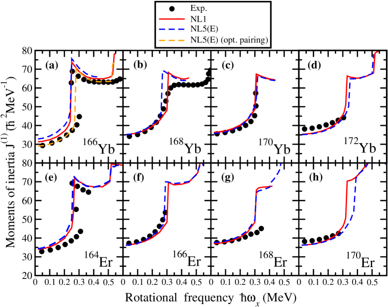
Figure 1: The kinematic MOIs $J^{(1)}$ for the GSBs of ^{166,168,170,172}Yb (upper panels) and ^{164,166,168,170}Er (lower panels), obtained in the CRHB+LN calculations with the CEDFs NL1 Reinhard et al. (1986) (red solid lines) and NL5(E) Agbemava et al. (2019) (blue dashed lines), compared to the experimental data (black solid circles). The latter are taken from Refs. Singh and Chen (2018); Baglin (2008a, 2010); Baglin et al. (2018); Firestone et al. (1999). Orange dashed line in panel (a) shows the results obtained with the NL5(E) CEDF and scaling factor $f$ of Gogny pairing fitted in such a way that it exactly reproduces experimental MOI of ¹⁶⁶Yb GSB at $\hbar\omega_{x}=0.05$ MeV.

Figure 1 compares experimental and theoretical MOIs obtained in the CRHB+LN calculations with the CEDFs NL1 and NL5(E). It can be seen that the results of the calculations for both functionals are close to each other. They also reproduce the experimental MOIs quite well. Note that the CRHB+LN, cranking CDFT-SLAP and PNC-CSM calculations are performed as a function of rotational frequency. Thus, they cannot predict or describe the back-sloping part of the backbending curve. However, they can reproduce an average frequency of backbending defined as $\hbar\omega_{\rm ave}=\frac{1}{2}(\hbar\omega_{1}+\hbar\omega_{2})$ where $\hbar\omega_{1}$ corresponds to the frequency at which the MOI curve bends backward and $\hbar\omega_{2}$ to the frequency at which the MOI curve bends forward.

There is only a small difference in the band crossing frequencies for the $N=98$ (¹⁶⁶Er and ¹⁶⁸Yb) and $N=102$ (¹⁷⁰Er and ¹⁷²Yb) isotones obtained in the calculations with the NL1 and NL5(E) functionals (see Fig. 1). In the $N=98$ isotones [Figs. 1(b) and (f)], the calculated first upbending takes place at somewhat lower frequencies for NL5(E) as compared with NL1. On the contrary, the situation is reversed in the $N=102$ isotones [Figs. 1(d) and (h)]. In the $N=96$ (¹⁶⁴Er and ¹⁶⁶Yb) isotones, the first band crossing is calculated at $\hbar\omega_{x}\approx 0.25$ MeV. The calculated first band crossing frequency gradually increases with increasing neutron number and it reaches $\hbar\omega_{x}\approx 0.32$ MeV in the $N=102$ (¹⁷⁰Er and ¹⁷²Yb) isotones. The calculated first upbendings are very sharp in the CRHB+LN calculations for both functionals. Experimental data show that sharp backbendings exist in ^166,170Yb [Figs. 1(a) and (c)] and ¹⁶⁴Er [Fig. 1(e)], while the upbendings in ¹⁶⁸Yb [Fig. 1(b)] and ¹⁶⁶Er [Fig. 1(f)] are somewhat smoother as compared with calculations. Note that for the ^170,172Yb [Figs. 1(b) and (d)] and ^166,168,170Er [Figs. 1(f), (g) and (h)] nuclei the $s$-bands have not been observed experimentally. Therefore, further experiments are needed to verify the predicted upbending features of these nuclei.

It can be seen in Fig. 1(b) that a second upbending in ¹⁶⁸Yb is observed experimentally at $\hbar\omega_{x}\sim 0.58$ MeV. In this nucleus, the CRHB+LN calculations for both functionals do not converge above $\hbar\omega_{x}=0.45$ MeV. This numerical instability is most likely caused by the competition of different configurations located at comparable energies in the region of second band crossing. Indeed, the CRHB+LN calculations provide converged solutions at frequencies $\hbar\omega_{x}\sim 0.6$ MeV in most of the nuclei under consideration even if the pairing is extremely weak. These solutions are not shown in Fig. 1 if there is non-convergence in the region of second band crossing. Thus, this non-convergence should not necessary be a manifestation of the deficiencies of the LN method. Note that similar situation with non-convergence of the CRHB+LN solutions in the region of second band crossing has been observed also in rotational structures of some actinides and light superheavy nuclei (see Ref. Afanasjev and Abdurazakov (2013)).

Note that the CRHB+LN calculations converge in most of even-even nuclei. For example, they predict second upbending in ¹⁶⁶Yb and ^164,166Er nuclei at $\hbar\omega_{x}\approx 0.53$ MeV [see Figs. 1(a), (e) and (f)]; these nuclei are the neighbors of ¹⁶⁸Yb. These frequencies are only slightly lower than the one at which experimental second upbending is seen in ¹⁶⁸Yb. In addition, second upbendings are predicted in ¹⁷²Yb and ¹⁷⁰Er [see Figs. 1(d) and (h)]. In the CRHB+LN calculations, both sharp and gradual second upbendings appear in this mass region contrary to only sharp first upbendings.

The differences (especially those related to different crossing frequencies) in the model predictions obtained with the NL1 and NL5(E) CEDFs are attributable to the differences in the underlying single-particle structure and, in particular, to the energies with respect of vacuum of aligning orbitals which are responsible for band crossing (see Fig. 7 below). As illustrated by orange dashed line in Fig. 1(a), some additional improvement in the description of experimental data could be obtained by further optimization of pairing. In the ‘NL5(E) (opt. pairing)’ calculations, the scaling factor $f$ of the Gogny pairing is selected in such a way that it reproduces exactly the experimental MOI at $\hbar\omega_{x}=0.05$ MeV. This leads to both much better description of absolute values of MOI before and after first band crossing in ¹⁶⁶Yb and the frequency of first band crossing.

All these results demonstrate that the LN method is a reasonably good approximation to exact particle-number conserving method at least for the yrast bands in even-even nuclei. It allows to avoid the pairing collapse (appearing in the standard BCS or HFB approaches) in significant frequency range. This collapse in the CRHB+LN calculations takes place only at very high rotational frequencies where the pairing is very weak. Note that at these frequencies, the calculations without pairing represent a feasible alternative for the analysis of rotational properties. In addition, at these frequencies such calculations are to a large degree free from numerical or convergence problems existing both in the CRHB+LN and the cranking CDFT-SLAP approaches.

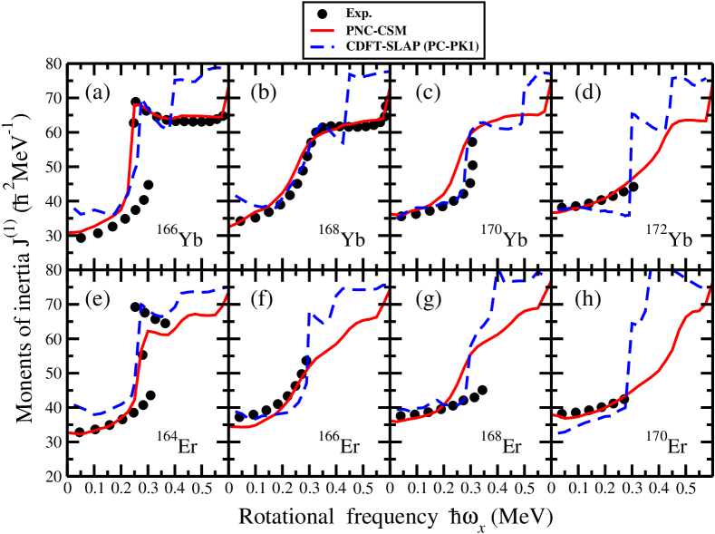
Figure 2: The same as in Fig. 1 but for the results of the calculations obtained with cranking CDFT-SLAP (blue dashed lines) and PNC-CSM (red solid lines). The PC-PK1 functional Zhao et al. (2010) is used in the cranking CDFT-SLAP calculations.

For a detailed comparison of the description of rotational properties by different models, Fig. 2 presents the results of the calculations obtained by the cranking CDFT-SLAP and PNC-CSM for the same set of nuclei as shown in Fig. 1. These two models with exact particle-number conservation can reproduce the experimental data reasonably well. On average, the PNC-CSM reproduces the experimental MOIs better than the cranking CDFT-SLAP. On the contrary, the accuracy of the description of available experimental data by PNC-CSM and CRHB+LN models is on average comparable (compare Figs. 2 and 1). However, in general the predictions of these two models differ above $\hbar\omega_{x}>0.35$ MeV, especially in the Er isotopes.

The cranking CDFT-SLAP and CRHB+LN calculations share the common feature: most of first band crossings are sharp and take place around $\hbar\omega_{x}\sim 0.3$ MeV (see Figs. 1 and 2). On the contrary, in the PNC-CSM calculations the upbendings are sharp only for the $N=96$ isotones and they become more gradual with increasing neutron number. As mentioned in Refs. Wu and Zeng (1991a, b), the yrast-yrare interaction strength, responsible for band crossing features, depends sensitively on the occupation number distribution in the high-$j$ orbitals. As a result, the differences in band crossing features may come from the differences in the single-particle structure obtained by different models and the rate of their change in the band crossing region. For example, the deformations (and thus the mean field) are fixed in the PNC-CSM calculations. Thus, the single-particle structure changes gradually at the band crossing region and the upbendings tend to be more gradual. On the contrary, the mean field is defined fully self-consistently with rotational frequency in the CDFT-based calculations. As a consequence, the upbendings may lead to a substantial change of equilibrium deformation and thus to significant changes of the single-particle structure (see the discussion of the Figs. 4 and 7 below). Therefore, the interaction between the the GSB and $s$-band configurations in the band crossing region may be weak, which will lead to a sharp upbending in the cranking CDFT-SLAP and CRHB+LN calculations.

It is necessary to recognize that spectroscopic quality of CEDFs is lower than that of phenomenological potentials such as Nilsson potential Afanasjev and Shawaqfeh (2011); Dobaczewski et al. (2015). This is because CEDFs are fitted only to bulk properties (such as nuclear masses and charge radii in the case of the PC-PK1 functional) and no information on single-particle energies is used in the fitting protocols. On the contrary, the set of Nilsson parameters used in the present manuscript is fitted to the energies of the 1-qp states in the mass region under study. These facts may also contribute into the differences, related to the first band crossing features, existing between CDFT-based and Nilsson potential based models. Moreover, the differences in the type of employed pairing force (Gogny pairing in CRHB+LN versus monopole pairing in cranking CDFT-SLAP and versus monopole+quadrupole pairing in PNC-CSM) and the way particle number projection is treated also can play a role in above discussed differences between model predictions.

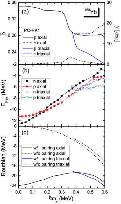
Figure 3: The evolution of the deformation parameters ($\beta,\gamma$) [panel (a)], proton and neutron pairing energies [panel (b)], and total Routhians [panel (c)] with rotational frequency obtained in the cranking CDFT-SLAP calculations with CEDF PC-PK1 for two competing at high spin minima in ¹⁶⁸Yb. One minimum [denoted as ‘axial’] has axial or near-axial shapes, while another [denoted as ‘triaxial’] corresponds to triaxial shapes with $\gamma\approx 18^{\circ}$. The results of the calculations with and without pairing are denoted as ‘w/’ and ‘w/o’, respectively. Note that the same constant energy is subtracted in all total Routhians, which sets the total Routhian of the minimum with near-axial shape in the calculations without pairing to zero at $\hbar\omega_{x}=0$.

The PNC-CSM calculations predict the existence of a sharp second upbending in all Yb and Er isotopes at rotational frequency $\hbar\omega_{x}~{}\sim 0.58$ MeV (see Fig. 2). For the case of ¹⁶⁸Yb, this is consistent with available experimental data [see Fig. 2(b)]. In the cranking CDFT-SLAP calculations, the second upbending takes place at substantially lower frequencies as compared with the PNC-CSM and CRHB+LN results. This is due to the appearance of triaxial minimum with $\gamma\approx 18^{\circ}$ at high rotational frequencies in the cranking CDFT-SLAP calculations which competes with near-axial minimum. Fig. 3 shows the evolution of deformation parameters ($\beta,\gamma$), proton and neutron pairing energies, and total Routhians with rotational frequency obtained in the cranking CDFT-SLAP calculations with PC-PK1 for these two minima in ¹⁶⁸Yb. The ground state of ¹⁶⁸Yb is axially deformed. With increasing rotational frequency, the triaxial deformation $\gamma$ gradually increases but still remains relatively small. A triaxial minimum with the energy comparable to the one of near-axial minimum develops at $\hbar\omega_{x}\approx 0.35$ MeV after the first band crossing. It can be seen in Fig. 3(a) that this minimum has substantially smaller quadrupole deformation $\beta$ than the near-axial one and that the triaxial deformation increases from $\gamma\approx 15^{\circ}$ at $\hbar\omega_{x}\approx 0.35$ MeV to $\gamma\approx 20^{\circ}$ at $\hbar\omega_{x}=0.60$ MeV. Fig. 3(c) shows the total Routhians of calculated configurations. One can see that the total Routhian of near-axial minimum is energetically favoured as compared with the one of triaxial minimum in the calculations without pairing. However, in the calculations with pairing the triaxial minimum becomes energetically favoured at $\hbar\omega_{x}>0.4$ MeV because pairing energies in this minimum are substantially larger than those in near-axial one [see Fig. 3(b)]. The energies of these two minima are very close to each other in some rotational frequency range. Thus, the self-consistent calculations should be carefully carried out to ensure that the real global minimum is found. Note that the competition of these two minima depends not only on the details of the pairing interaction, but also on underlying single-particle structure.

The calculated MOIs obtained in the cranking CDFT-SLAP are less smooth as compared with the CRHB+LN ones. This is because in the cranking CDFT-SLAP, the many-body Hamiltonian is diagonalized directly in the MPC space. As a consequence, the eigenstate [Eq. (6)] is no longer a Slater determinant but the superposition of many Slater determinants. When investigating heavy nuclei with high single-particle level densities, there may exist several low-lying MPCs with very close excitation energies, especially when triaxial deformation appears. With different initial mean field, the near degeneracy of these MPCs may lead the cranking CDFT-SLAP calculations to converge to somewhat different minima, which have slightly different expansion coefficients $C_{i}$ in the eigenstate [Eq. (6)]. As a consequence, the change of rotational frequency can trigger minor discontinuities in the occupation probabilities of the single-particle levels located in the vicinity of the Fermi level. If some of these affected states are high-$j$ ones, this can lead to small fluctuations in MOIs calculated as a function of rotational frequency. This defect of cranking CDFT-SLAP can be avoided by using the single-particle level tracking technique and considering the overlap between two eigenstates calculated at adjacent rotational frequencies Meng et al. (2006c); Shi et al. (2018). However, it is too time-consuming for a systematic investigation of these heavy nuclei.

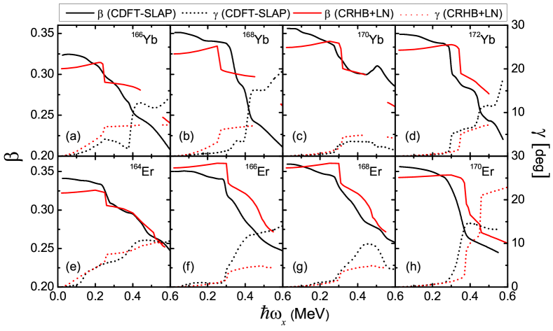
Figure 4: The evolution of deformation parameters $\beta$ and $\gamma$ with rotational frequency in even-even nuclei under study obtained in the cranking CDFT-SLAP (solid lines) and CRHB+LN (dotted lines) calculations. The cranking CDFT-SLAP and CRHB+LN calculations are performed with the PC-PK1 and NL5(E) CEDFs, respectively.

Figure 4 shows the evolution of deformation parameters $\beta$ and $\gamma$ with rotational frequency obtained in two CDFT-based approaches. One can see that in general it is similar in both approaches. However, some differences are also present. At low frequencies, all nuclei are axially symmetric and with exception of ¹⁶⁶Er quadrupole deformations $\beta$ obtained in cranking CDFT-SLAP calculations are somewhat larger than those calculated in the CRHB+LN approach. The triaxiality gradually increases with increasing rotational frequency up to first band crossing in both calculations. However, in this frequency range the behaviour of calculated quadrupole deformations is different in the cranking CDFT-SLAP and CRHB+LN approaches. With increasing rotational frequency up to first band crossing, the $\beta$ values gradually decrease/increase in the cranking CDFT-SLAP/CRHB+LN calculations. Similar trend of the evolution of the $\beta$ values with increasing rotational frequency has also been seen in other CRHB+LN calculations Afanasjev et al. (1999b) and in non-relativistic cranked HFB calculations Terasaki et al. (1995). Both calculations show that in the first band crossing region of these nuclei the quadrupole deformations $\beta$ rapidly decrease and triaxial deformations $\gamma$ quickly increase. As a result of these significant deformation changes, the first band crossing is calculated in these two CDFT-based approaches to be sharp in most of the cases. The second band crossing leads to a further decrease of quadrupole deformation. With a pair of exception, it also triggers further increase of $\gamma$-deformation. Fig. 4 shows that both CDFT-based approaches predict significant triaxial deformation in these nuclei after the first band crossing. However, due to non-selfconsistent nature of the cranked shell model, the deformation is an input parameter in the PNC-CSM and the model does not allow the variation of deformation with spin. Thus, the axial symmetry is assumed in PNC-CSM calculations and the magnitude of the quadrupole deformation is taken from microscopic+macroscopic calculations which have similar structure of the single-particle potential. This is also consistent with experimental information on axial symmetry of the ground states in the rare-earth nuclei under study as well as with the results of two CDFT-based model calculations for the ground states. Note that the axial symmetry is adopted in absolute majority of cranked shell model calculations for the rare-earth nuclei under study (see, for example, Ref. Asgar et al. (2017)).

Some differences seen in the results of the cranking CDFT-SLAP and CRHB+LN calculations emerge from different employed CEDFs. For example, the $\gamma$-deformations of the solutions obtained after second band crossing are typically larger in the cranking CDFT-SLAP calculations. The pairing is weak in this frequency range and thus these differences could not be related to the treatment of pairing or the selection of the pairing force.

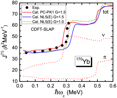
Figure 5: The MOIs of the GSB in ¹⁷⁰Yb obtained in the cranking CDFT-SLAP approach with the PC-PK1 and NL5(E) CEDFs. The contributions from proton and neutron subsystems to the MOIs obtained by PC-PK1 CEDF are shown by red dotted lines.

Figure 5 compares the results of cranking CDFT-SLAP calculations for the GSB in ¹⁷⁰Yb obtained with PC-PK1 and NL5(E) functionals. For the same pairing strength $G_{\rm n}=G_{\rm p}=1.5$ MeV, the MOIs obtained before first upbending with NL5(E) are somewhat smaller than those obtained with PC-PK1 and experimental ones. The calculations with NL5(E)/PC-PK1 slightly underestimate/overestimate the first band crossing frequency. Since the single-particle level structures located in the vicinity of the Fermi surface are different in those two CEDFs, the corresponding pairing strengths should not necessary be the same. The reduction of proton and neutron pairing strengths to $G_{\rm n}=G_{\rm p}=1.0$ MeV in the calculations with NL5(E) leads to a visible improvement of the description of experimental data (see Fig. 5). Note that the equilibrium deformations obtained in the calculations with PC-PK1 and NL5(E) are rather close to each other (see Fig. 6). It also can be seen that the first upbending is caused by the contribution from neutron subsystem, and the second upbending is caused by the contribution from proton subsystem. The same conclusion can be obtained for all even-even Er and Yb isotopes investigated in the present work by cranking CDFT-SLAP.

With the exception of first band crossing region, the behavior of the calculated MOIs presented in Fig. 5 are very close to each other. This is a consequence of the fact that the rotation is a collective phenomenon built on the contributions of many single-particle orbitals. As a result, minor differences in the single-particle structure introduced by the use of different functionals do not lead to substantial changes in MOIs. The only exception is the band crossing region which is defined by the alignment of selected pair of the orbitals and which depends more on the energies and alignment properties of this pair. Note that these features are also observed in the CRHB+LN calculations (see Fig. 1).

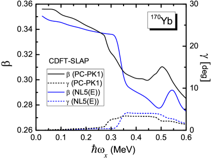
Figure 6: The evolution of deformation parameters $\beta$ and $\gamma$ with rotational frequency in ¹⁷⁰Yb obtained in the cranking CDFT-SLAP calculations with the NL5(E) and PC-PK1 CEDFs.

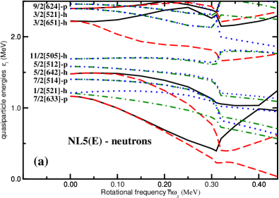
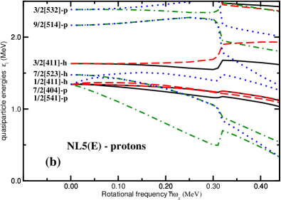
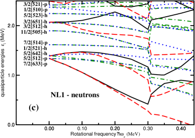
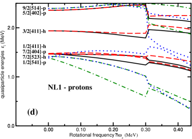
Figure 7: Neutron and proton quasiparticle energies (routhians) corresponding to the lowest configurations in ¹⁷⁰Yb obtained in the CRHB+LN calculations with NL5(E) (top panels) and NL1 (bottom panels) CEDFs. They are given along the deformation path of these configurations. Long-dashed, solid, dot-dashed and dotted lines indicate $(\pi=+,r=+i)$, $(\pi=+,r=-i)$, $(\pi=-,r=+i)$ and $(\pi=-,r=-i)$ orbitals, respectively. At $\Omega_{x}=0.0$ MeV, the quasiparticle orbitals are labeled by the asymptotic quantum numbers $[Nn_{z}\Lambda]\Omega$ (Nilsson quantum numbers) of the dominant component of the wave function. The letters ‘p’ and ‘h’ before the Nilsson labels are used to indicate whether a given routhian is of particle ($V^{2}<0.5$) or hole ($V^{2}>0.5$) type.

There is a substantial difference between the CRHB+LN and cranking CDFT-SLAP calculations in respect of the modifications of the calculated MOIs induced by the change of pairing strength. Fig. 5 shows that in the cranking CDFT-SLAP calculations with NL5(E) CEDF the reduction of monopole pairing strength by 1/3 leads only to moderate change in the MOI. Similar features have been observed in the cranking CDFT-SLAP calculations in other mass regions Liu (2019). On the contrary, the increase of scaling factor $f$ of the Gogny pairing force from 0.950 [blue dashed line in Fig. 1(a)] to 0.998 [orange dashed line in Fig. 1(a)] leads to larger changes in calculated MOI. In a similar fashion, the 10% change in pairing strength of the Gogny pairing force leads to a substantial changes in the calculated MOIs of superdeformed bands of the $A\sim 190$ mass region (see Fig. 12 in Ref. Afanasjev et al. (2000b)).

Figure 7 shows the quasiparticle routhians obtained in the CRHB+LN calculations with the NL1 and NL5(E) functionals. Although the energies of the routhians with the same structure are somewhat different in these functionals, there are large similarities in the general structure of the quasiparticle spectra obtained with these two functionals. For example, the alignments of the quasiparticle orbitals, reflected in the energy slope of their routhians as a function of rotational frequency, are very similar in both functionals. In addition, a similar sets of proton and neutron quasiparticle states appear in the vicinity of the Fermi level in these CEDFs. Moreover, in both functionals, the first paired band crossing is due to the alignment of the neutron $7/2^{+}[633]$ orbitals.

Figure 8 shows the single-particle routhians obtained in the cranking CDFT-SLAP calculations with PC-PK1 (upper panels) and NL5(E) (lower panels) functionals. There are large similarities between these two functionals in terms of the locations of similar set of the single-particle states in the vicinity of the Fermi level, the signature splittings of single-particle orbitals and their evolution with rotational frequency and the slope of the single-particle energies with rotational frequency. The comparison of the quasiparticle routhians shown in Figs. 7(a) and (b) and the single-particle routhians displayed in Figs. 8(b) and (d) allows to establish close correspondence between underlying single-particle structure obtained in the CRHB+LN and cranking CDFT-SLAP calculations with the NL5(E) functional. First band crossing leads to sharper changes in the energies of the proton and neutron single-particle states in the cranking CDFT-SLAP calculations with NL5(E) as compared with those for PC-PK1 (see Fig. 8). This is due to more drastic deformation changes obtained in the band crossing region in the calculations with NL5(E) (see Fig. 6). Note also that first band crossing takes place at higher frequency in NL5(E) than in PC-PK1.

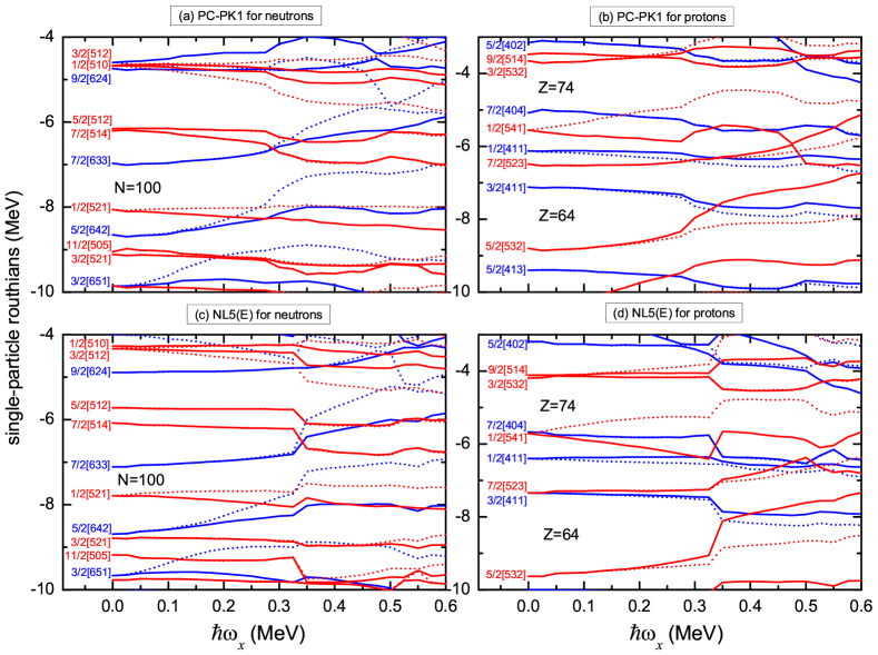
Figure 8: Neutron (left panels) and proton (right panels) single-particle routhians located in the vicinity of the Fermi level of the ¹⁷⁰Yb as a function of rotational frequency. Positive (negative) parity routhians are shown by blue (red) lines. Solid (dotted) lines are used for signature $\alpha=+1/2$ ($\alpha=-1/2$).

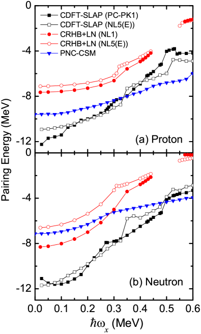
Figure 9: The neutron and proton pairing energies obtained in different calculations as a function of rotational frequency in ¹⁷⁰Yb.

Figure 9 shows the pairing energies for neutron and proton subsystems of ¹⁷⁰Yb as a function of rotational frequency obtained in the CRHB+LN, cranking CDFT-SLAP and PNC-CSM calculations. In general, both proton and neutron paring energies decrease with rotational frequency but even in the high-spin region they are still non-zero. Paired band crossings trigger some reduction of pairing energies and the change of the slope of pairing energies as a function of rotational frequency in the CDFT-based approaches. This is due to the change of the deformation of the mean-fields (see Fig. 4), the quasiparticle energies (see Fig. 7) in the CRHB+LN approach and the single-particle Routhians (see Fig. 8) in the cranking CDFT-SLAP approach taking place at the band crossings. Although the methods of the treatment of pairing correlations are exactly the same in the cranking CDFT-SLAP and PNC-CSM approaches, the variations of calculated pairing energies with rotational frequency are different. Contrary to the cranking CDFT-SLAP approach, the pairing energies decrease smoothly (even in the band crossing regions) with increasing rotational frequency in the PNC-CSM calculations. This is because the deformation is fixed in the PNC-CSM calculations. As a consequence, the single-particle levels change gradually with rotational frequency.

The calculated pairing energies depend both on theoretical framework as well as on the employed functional. The former dependence is due to different definitions of pairing energies in the CRHB+LN and cranking CDFT-SLAP approaches [compare Eqs. (26) and (17)] and the use of different pairing forces. The latter one enters through the dependence of pairing energies on the single-particle level density: in extreme case of large shell gap in the vicinity of the Fermi level there will be pairing collapse (see Ref. Shimizu et al. (1989)). For example, the CRHB+LN calculations with the NL1 and NL5(E) CEDFs are performed with comparable scaling factors $f$ of the Gogny pairing force. As a consequence, the similarity/difference of proton/neutron pairing energies in these calculations (see Fig. 9) are due to similarity/difference of the density of the proton/neutron single-particle states in the vicinity of respective Fermi levels (see Fig. 7). The situation is the same for the cranking CDFT-SLAP calculations with the PC-PK1 and NL5(E) CEDFs.

V Rotational properties of odd-proton nuclei ^{165,167,169,171}Tm

The rotational structures in odd-mass nuclei provide additional testing ground for theoretical approaches. In addition, they yield important information on underlying single-particle structure, thus providing an extra tool for the configuration assignment (see discussion in Sec. 4C of Ref. Afanasjev and Abdurazakov (2013)). However, the calculations in the cranking CDFT-SLAP and CRHB+LN approaches in such nuclei are extremely time consuming requiring significantly larger computational time than similar calculations in even-even nuclei.

In addition, there is a principal difference between the calculations of odd-mass nuclei in the CRHB+LN and the cranking CDFT-SLAP approaches. Such calculations in the CRHB+LN approach (as well as in non-relativistic HFB based approaches) employ blocking of specific single-particle orbital(s) for definition of nucleonic configurations. However, this frequently leads to numerical instabilities emerging from the interaction of blocked orbital with other single-particle orbital having the same quantum numbers and located close in energy (see Ref. Afanasjev and Abdurazakov (2013)). This deficiency is clearly seen in Fig. 10 where numerical convergence has been obtained in restricted frequency range for the $\pi 1/2^{+}[411]$ GSBs of odd-$A$ Tm isotopes and mostly for the $\alpha=+1/2$ signature. Note that calculated results are reasonably close to experimental data. Such numerical instabilities are also a reason why the calculations of rotational structures in odd-$A$ and odd-odd nuclei in relativistic and non-relativistic density functional theories are very rare. To our knowledge, such calculations have been performed so far only for few such nuclei (mostly for actinides) in Refs. Bender et al. (2003); O’Leary et al. (2003); Herzberg et al. (2009); Jeppesen et al. (2009); Afanasjev and Abdurazakov (2013) and mostly in the CRHB+LN framework.

On the contrary, the specific orbital is not blocked in shell-model based approaches and the process for calculating odd-$A$ nuclei is exactly the same as in even-even ones in the cranking CDFT-SLAP. Thus, there is no numerical convergence problems typical for HFB approaches. The analysis of the occupation probabilities of the single-particle levels located in the vicinity of the Fermi level allows to define nucleonic configurations. However, the problems similar to those revealed in the discussion of Fig. 3 and emerging from the convergence of the calculations to slightly different minima exist also in odd-$A$ nuclei. They increase computational time and require substantial time for the analysis of the calculations and configuration assignment to observed band.

Figure 10 compares experimental data on MOIs of the GSB $\pi 1/2^{+}[411]$ in odd-$A$ Tm isotopes with the results of the calculations of the CDFT-based models. In the cranking CDFT-SLAP calculations, the convergence can be obtained up to very high frequency in all nuclei under study (see Fig. 10). The frequency of first band crossing and the MOIs immediately after it are very close to experimental data in ¹⁶⁵Tm. However, at low frequency the MOIs are somewhat overestimated in the calculations and the signature splitting is not reproduced. The latter feature is due to small signature splitting of the $\pi 1/2^{+}[411]$ orbital obtained in the cranking CDFT-SLAP calculations (see Fig. 8). In addition, the cranking CDFT-SLAP calculations predict a second upbending at $\hbar\omega_{x}\sim 0.4$ MeV (similar to the one predicted in even-even nuclei in Fig. 2), which is not observed in experiment. In ^167,169Tm nuclei, the calculated results are similar to those obtained in ¹⁶⁵Tm.

The MOIs of opposite signatures of the $\pi 1/2^{+}[411]$ band in ¹⁶⁵Tm are rather well reproduced before band crossing in the CRHB+LN calculations with the NL5(E) functional (see Fig. 10). However, at higher frequency only the $\alpha=+1/2$ branch converges in the CRHB+LN calculations and only for rotational frequencies $\hbar\omega_{x}<0.38$ MeV. For this branch, the calculated upbending takes place at the frequency which is close to medium frequency of experimental backbending. In ¹⁶⁷Tm, the calculations converge only up to $\hbar\omega_{x}\sim 0.19$ MeV. The signature splitting is rather well reproduced but the calculations somewhat underestimate the experimental values of MOIs. In ¹⁶⁹Tm, the CRHB+LN calculations converge only for $\alpha=+1/2$ branch and only for low frequencies. Here the results of the calculations are very close to experimental data. Note that no convergence for the $\pi 1/2^{+}[411](\alpha=\pm 1/2)$ bands have been obtained in the CRHB+LN calculations with the NL1 functional. The close energies of the $\pi 1/2^{+}[411]$ and $\pi 7/2^{+}[404]$ quasiparticle orbitals [see Figs. 7 (b) and (d)], leading to a substantial interaction between them, is the most likely source of the convergence problems observed in the CRHB+LN calculations.

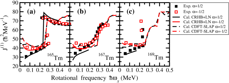
Figure 10: The MOIs of the GSB $\pi 1/2^{+}[411]$ in odd-$A$ Tm isotopes. Experimental data, taken from Refs. Jensen et al. (2001); Burns et al. (2005); Asgar et al. (2017) are compared with the results of the CRHB+LN with NL5(E) and the cranking CDFT-SLAP calculations with PC-PK1.

In the light of time-consuming nature of the calculations within the CDFT-based approaches and above discussed technical difficulties, the systematic investigation of the properties of odd-proton nuclei ^{165,167,169,171}Tm will be performed here only in the PNC-CSM framework.

Table 5: The comparison between experimental and PNC-CSM results for bandhead energies of low-lying 1- and 3-qp states in ^{165,167,169,171}Tm. $E_{\rm th}$, $E_{\rm stand}$, and $E_{\rm A150}$ denote the calculated energies obtained with different sets of the Nilsson parameters. Here, ‘th’, ‘stand’ and ‘A150’ stand for the parameters adopted in the present work, derived for global description in Ref. Bengtsson and Ragnarsson (1985) (frequently called ‘standard Nilsson parameters’) and defined from high spin properties in the $A\sim 150$ mass region in Ref. Bengtsson (1990), respectively. The experimental data are taken from Refs. Jain et al. (2006); Baglin (2000, 2008b); Baglin and McCutchan (2018). $K^{\pi}=17/2^{+}$ and $K^{\pi}=17/2^{-}$ in ¹⁶⁵Tm denote two 3-qp states with the configuration $\pi 7/2^{+}[404]\otimes\nu^{2}5/2^{-}[523]5/2^{+}[642]$ and $\pi 7/2^{-}[523]\otimes\nu^{2}5/2^{-}[523]5/2^{+}[642]$, respectively.

Nuclei	Configuration	$E_{\rm exp}$ (keV)	$E_{\rm th}$ (keV)	$E_{\rm stand}$ (keV)	$E_{\rm A150}$ (keV)
165Tm	$\pi 1/2^{+}[411]$	0	0	0	0
165Tm	$\pi 7/2^{+}[404]$	80	93	393	482
165Tm	$\pi 7/2^{-}[523]$	160	138	325	12
165Tm	$\pi 5/2^{+}[402]$	315	414	722	465
165Tm	$\pi 3/2^{+}[411]$	416	1312	1168	1488
165Tm	$\pi 9/2^{-}[514]$	831	791	899	1272
165Tm	$17/2^{+}$	1634	1676	2020	2065
165Tm	$17/2^{-}$	1741	1721	1952	1595
167Tm	$\pi 1/2^{+}[411]$	0	0	0	0
167Tm	$\pi 7/2^{+}[404]$	180	335	549	664
167Tm	$\pi 7/2^{-}[523]$	293	224	319	45
167Tm	$\pi 5/2^{+}[402]$	558	680	859	618
167Tm	$\pi 3/2^{+}[411]$	471	1451	1193	1336
167Tm	$\pi 9/2^{-}[514]$	928	873	899	1284
169Tm	$\pi 1/2^{+}[411]$	0	0	0	0
169Tm	$\pi 7/2^{+}[404]$	316	542	733	826
169Tm	$\pi 7/2^{-}[523]$	379	393	450	30
169Tm	$\pi 5/2^{+}[402]$	782	916	1078	782
169Tm	$\pi 9/2^{-}[514]$	1152	968	976	1226
171Tm	$\pi 1/2^{+}[411]$	0	0	0	0
171Tm	$\pi 7/2^{+}[404]$	636	655	856	945
171Tm	$\pi 7/2^{-}[523]$	425	465	500	172
171Tm	$\pi 5/2^{+}[402]$	912	1062	1254	899
171Tm	$\pi 3/2^{+}[411]$	676	1560	1245	1442

Table 5 shows the comparison between the experimental and calculated bandhead energies of the 1- and 3-qp states in ^{165,167,169,171}Tm. Note that the bandhead energies of the $\pi 1/2^{-}[541]$ states are not shown in this table due to the following reasons. First, the deformation of this state is larger than that for other states because it has strong deformation driving effect Nazarewicz et al. (1990); Warburton et al. (1995). Second, because of strong decoupling effect arising from Coriolis interaction the $I=5/2\hbar$ state is located lower in energy in experiment than the bandhead with spin $I=1/2\hbar$.

One can see that calculated energies obtained with ‘stand’ and ‘A150’ sets of the Nilsson parameters (see caption of Table 5 for details) cannot reproduce experimental data well. This is especially true for the excitation energies of the $\pi 7/2^{+}[404]$ state, which are calculated too high in energy as compared with experimental data. In addition, the sequence of the $\pi 7/2^{+}[404]$ and $\pi 5/2^{+}[402]$ states is reversed as compared with experiment when the ‘A150’ set of the Nilsson parameters is used. Note also that all three employed sets of the Nilsson parameters overestimate experimental excitation energies of the $\pi 3/2^{+}[411]$ states in all considered Tm isotopes. The two 3-qp states observed in ¹⁶⁵Tm are reproduced very well by the Nilsson parameter set ‘th’ adopted in the present work. On the contrary, the energies of these states calculated with ‘stand’ and ‘A150’ sets of the parameters deviate from experiment by 200-300 keV. These results indicate that in general adopted set of the Nilsson parameters improves a description of experimental data as compared with that obtained with ‘stand’ and ‘A150’ sets of the parameters and provides a reasonably accurate single-particle structure. This is important for a detailed investigation of rotational properties and band crossing features of the nuclei under study.

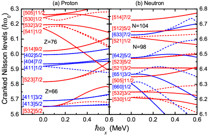
Figure 11: Proton [panel (a)] and neutron [panel (b)] single-particle routhians located in the vicinity of the Fermi level of the ¹⁶⁵Tm nucleus as a function of rotational frequency $\hbar\omega_{x}$. Positive (negative) parity routhians are shown by blue (red) lines. Solid (dotted) lines are used for signature $\alpha=+1/2$ ($\alpha=-1/2$).

Underlying single-particle structure and its evolution with rotational frequency is exemplified in Fig. 11; similar structures are also seen in the ^167,169,171Tm nuclei. At low rotational frequencies there exist a proton shell gap at $Z=76$ and two neutron shell gaps at $N=98$ and 104. With increasing rotational frequency these gaps either disappear or get substantially reduced. In the Tm isotopes of interest, with increasing neutron number the neutron Fermi level is shifted up from $N=96$ to $N=102$. Both the magnitude of the shell gaps and the position of the Fermi level may affect the backbendings/upbendings in these Tm isotopes. Note that the total Routhian surface (TRS) calculations of Ref. Asgar et al. (2017) with Woods-Saxon potential show small neutron shell gap at $N=102$ instead of the $N=104$ one present in our calculations.

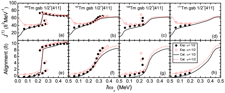
Figure 12: The experimental and calculated MOIs $J^{(1)}$ (upper panels) and alignments (lower panels) of the GSBs $\pi 1/2^{+}[411]$ in ^{165,167,169,171}Tm. The experimental MOIs and alignments are displayed by black solid and red open circles for the $\alpha=+1/2$ and $\alpha=-1/2$ branches of rotational band, respectively. Corresponding calculated values are displayed by black solid ($\alpha=+1/2$) and red dotted ($\alpha=-1/2$) lines. The experimental data are taken from Refs. Jensen et al. (2001); Burns et al. (2005); Asgar et al. (2017); Walker et al. (2009). The alignments $i=\langle J_{x}\rangle-\omega_{x}J_{0}-\omega_{x}^{3}J_{1}$ and the Harris parameters $J_{0}=35~{}\hbar^{2}$MeV^-1 and $J_{1}=43~{}\hbar^{4}$MeV^-3 are taken from Ref. Asgar et al. (2017).

Figure 12 displays the comparison between experimental and calculated MOIs and alignments for the GSBs $\pi 1/2^{+}[411]$ in ^{165,167,169,171}Tm. One can see that in general the variation of the experimental MOIs, alignments and signature splittings with rotational frequency are reproduced reasonably well in the PNC-CSM calculations. In experimental data, sharp backbendings exist in the ^165,169Tm nuclei but the upbending is quite smooth and moderate in ¹⁶⁷Tm. Smooth upbending in ¹⁶⁷Tm is rather well reproduced by the PNC-CSM calculations [Figs. 12(b) and (f)]. In ¹⁶⁵Tm, the calculations predict a sharp upbending (consistent with the backbending in experiment), and the frequency of which is close to that of experimental backbending [Figs. 12(a) and (e)]. However, the PNC-CSM calculations predict a smooth and moderate upbending instead of a sharp backbending in ¹⁶⁹Tm [Figs. 12(c) and (g)]. Note that in the calculations the alignment process is more smooth in ¹⁷¹Tm as compared with ¹⁶⁷Tm [compare Figs. 12(d) and (h) with Figs. 12(b) and (f)]. However, there are no enough experimental data to confirm these predictions. These results are quite similar to those obtained in the TRS calculations of Ref. Asgar et al. (2017). It should be noted that in Ref. Asgar et al. (2017), the calculated interaction strength at the band crossing in ¹⁶⁹Tm ($V_{\rm int}=10$ keV) is smaller than that in ¹⁶⁵Tm ($V_{\rm int}=20$ keV). This indicates that the backbending in ¹⁶⁹Tm is sharper than the one in ¹⁶⁵Tm, which is inconsistent with experimental data.

In the CSM approach, the band crossing features depend on the interaction strength $V_{\rm int}$ between the configurations corresponding to 1-qp band before band crossing and 3-qp configuration after band crossing. A sharp backbending will appear for small $V_{\rm int}$ values. A large shell gap will also make the band crossing more smooth. In Ref. Asgar et al. (2017), a smaller interaction strength and a smaller shell gap in ¹⁷¹Tm than in ¹⁶⁷Tm are predicted by TRS calculations. As a result, TRS calculations predict sharper upbending in ¹⁷¹Tm than in ¹⁶⁷Tm.

Considering the similarity of equilibrium deformations of these nuclei (see Table 3) the differences in their alignment features have to be related to the evolution of underlying neutron single-particle structure and the changes in the position of neutron Fermi level with the increase of neutron number. These factors and their impact on rotational properties and band crossing features are discussed in detail below.

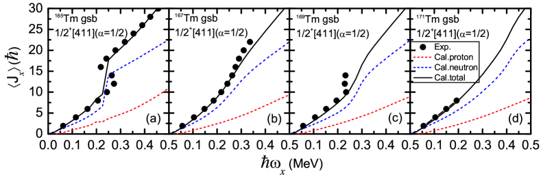
Figure 13: The experimental (solid circles) and calculated (black solid line) angular momentum alignments $\langle J_{x}\rangle$ for the GSBs $\pi 1/2^{+}[411](\alpha=1/2)$ in ^{165,167,169,171}Tm. Proton and neutron contributions to $\langle J_{x}\rangle$ are shown by red and blue dashed lines, respectively. Theoretical values are obtained in the PNC-CSM calculations. Note that contrary to bottom panels of Fig. 12, smoothly increasing part of the alignment represented by the Harris formula is not subtracted in this figure.

Experimental and calculated angular momentum alignments $\langle J_{x}\rangle$ for the ground state $\pi 1/2^{+}[411](\alpha=1/2)$ bands in ^{165,167,169,171}Tm as well as respective calculated proton and neutron contributions to $\langle J_{x}\rangle$ are shown in Fig. 13. Note that contrary to bottom panels of Fig. 12, smoothly increasing part of the alignment represented by the Harris formula is not subtracted in Fig. 13. The latter figure clearly shows that similar to even-even nuclei the first backbendings or upbendings emerge from the band crossings in neutron subsystem. As a result, we focus only on neutron subsystem in the discussion below.

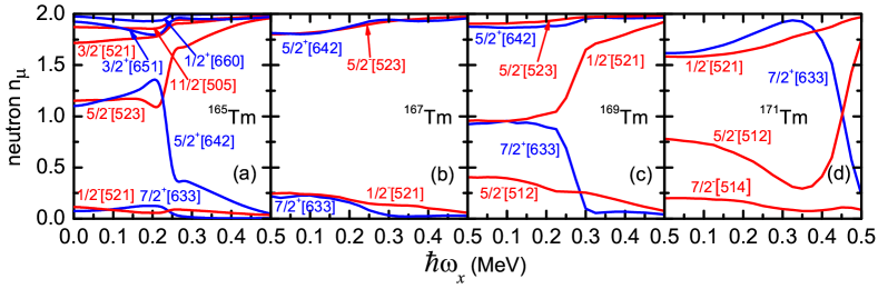
Figure 14: The occupation probabilities $n_{\mu}$ of neutron orbitals $\mu$ (counting both $\alpha=\pm 1/2$ signatures together so that the maximum occupation probability is 2.0) located close to the Fermi level in the GSBs of ^{165,167,169,171}Tm. The positive (negative) parity levels are shown by blue (red) lines. The Nilsson levels located far above (with $n_{\mu}\sim 0$) and far below (with $n_{\mu}\sim 2.0$) the Fermi level are not shown.

Figure 14 shows the occupation probabilities $n_{\mu}$ of neutron orbitals $\mu$ located close to the Fermi level in the GSBs of ^{165,167,169,171}Tm. In the PNC-CSM calculations, the particle-number is conserved from beginning to the end, whereas the occupation probabilities $n_{\mu}$ of the orbitals change with rotational frequency. By examining the variations of the occupation probabilities with rotational frequency, one can get detailed insight into the backbending or upbending mechanisms. One can see from Fig. 14(a) that in ¹⁶⁵Tm at rotational frequency $\hbar\omega_{x}\sim 0.25$ MeV, the occupation probability $n_{\mu}$ of the neutron $\nu 5/2^{+}[642]$ orbital drops sharply from 1.4 down to 0.3, while that of the $\nu 5/2^{-}[523]$ orbital increases sharply from 1.0 up to 1.7. On the contrary, the occupation probabilities of other orbitals (such as $\nu 3/2^{-}[521]$, $\nu 3/2^{+}[651]$ and $\nu 7/2^{+}[633]$) change only modestly in the frequency range corresponding to the backbending. This indicates that the main contribution to sharp backbending observed in ¹⁶⁵Tm comes from the neutron $\nu 5/2^{+}[642]$ orbital emerging from the spherical $i_{13/2}$ subshell (see also the discussion below). Other deformed orbitals emerging from this subshell (such as $\nu 3/2^{+}[651]$ and $\nu 7/2^{+}[633]$) provide significantly smaller contribution to this backbending.

In the case of ¹⁶⁷Tm, the orbitals above (below) the Fermi level are nearly empty (occupied) [see Fig. 14(b)] due to the presence of a large shell gap at $N=98$ [see Fig. 11(b)]. The occupation probabilities of the displayed orbitals are nearly constant before and after rotational frequency range of $\hbar\omega_{x}=0.2-0.3$ MeV corresponding to smooth upbending in this nucleus. The absence of sharp change of the occupation of the orbitals means that no sharp backbending exists in ¹⁶⁷Tm. Gradual deoccupation of the $\nu 7/2^{+}[633]$ orbital and gradual occupation of the $\nu 5/2^{+}[642]$ and $\nu 5/2^{-}[523]$ orbitals in above mentioned frequency range is mostly responsible for the smooth upbending in this nucleus.

The situation changes in ¹⁶⁹Tm; the occupation probability $n_{\mu}$ of the $\nu 7/2^{+}[633]$ orbital decreases from 0.7 down to 0.1 and the one of the $\nu 1/2^{-}[521]$ orbital increases from 1.2 up to 1.7 on going from $\hbar\omega_{x}\approx 0.25$ MeV up to $\hbar\omega_{x}\approx 0.3$ MeV [see Fig. 14(c)]. Therefore, the backbending in ¹⁶⁹Tm comes from rapid deoccupation of the $\nu 7/2^{+}[633]$ orbital. Note that the change of the occupation probabilities $n_{\mu}$ of the orbitals of interest in ¹⁶⁹Tm is not as sharp as that in ¹⁶⁵Tm and with a higher $\Omega$ value in $\nu 7/2^{+}[633]$ as compared with $\nu 5/2^{+}[642]$, it is understandable that the backbending in ¹⁶⁹Tm is somewhat weaker than in ¹⁶⁵Tm.

For ¹⁷¹Tm the occupation probability $n_{\mu}$ of the $\nu 7/2^{+}[633]$ orbital decreases gradually from 1.9 down to 0.2, while that for the $\nu 5/2^{-}[512]$ orbital increases gradually from 0.3 up to 1.7 in the frequency range $\hbar\omega_{x}=0.35-0.50$ MeV. Thus, the calculations predict a smooth upbending centered at $\hbar\omega_{x}\sim 0.42$ MeV, which takes places at higher frequency as compared with backbendings/upbendings in lower $N$ Tm isotopes.

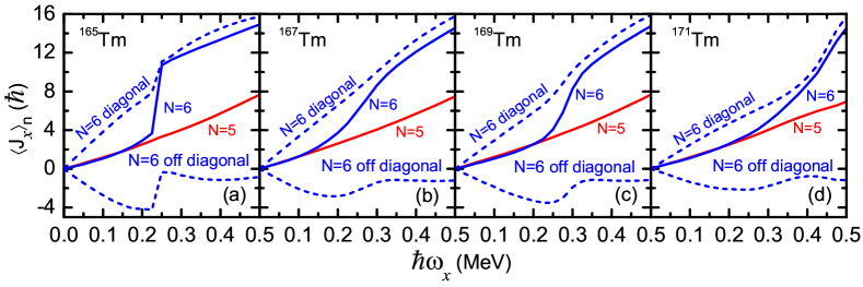
Figure 15: The contributions of neutron $N=5,6$ major shells to the angular momentum alignment $\langle J_{x}\rangle$ of the GSBs in ^{165,167,169,171}Tm. Solid blue and red lines are used for the $N=5$ and $N=6$ shells, respectively. The contributions of diagonal [$\Sigma_{\mu}j_{x}(\mu)$] and off-diagonal [$\Sigma_{\mu<\nu}j_{x}(\mu\nu)$] parts in Eq. (10) coming from the neutron $N=6$ major shell are shown by blue dashed lines.

The contributions of neutron $N$ = 5 and 6 major shells to the angular momentum alignment $\langle J_{x}\rangle$ of the GSBs in ^{165,167,169,171}Tm are shown in Fig. 15. In all these Tm isotopes the backbendings or upbendings emerge from the contributions of the neutron $N=6$ major shell since at the frequencies corresponding to this phenomena these contributions increase either drastically or gradually above the trend seen at low frequencies. On the contrary, the $N=5$ contributions to $\langle J_{x}\rangle$ form almost straight lines as a function of rotational frequency [see Fig. 15]. In ¹⁶⁵Tm, sharp backbending emerges predominantly from the $N=6$ shell off-diagonal contribution to $\langle J_{x}\rangle$; however, smaller diagonal contribution is still present [see Fig. 15(a)]. In the case of ¹⁶⁷Tm, smooth upbending almost fully comes from the $N=6$ shell off-diagonal contribution to $\langle J_{x}\rangle$ [see Fig. 15(b)]. Upbending in ¹⁶⁹Tm again dominates by the $N=6$ shell off-diagonal contribution to $\langle J_{x}\rangle$ but relatively small diagonal contribution is still visible [see Fig. 15(c)]. The balance of diagonal and off-diagonal contributions to $\langle J_{x}\rangle$ becomes more equal in smooth upbending of ¹⁷¹Tm [see Fig. 15(d)].

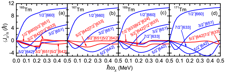
Figure 16: The contributions of the neutron $N=6$ orbitals to the angular momentum alignments of the GSBs in ^{165,167,169,171}Tm. Blue and red lines display the diagonal [$j_{x}(\mu)$] and off-diagonal [$j_{x}(\mu\nu)$] terms in Eq. (10), respectively.

In order to have a more detailed understanding of the level crossing mechanism, the contributions of the neutron $N=6$ orbitals to the angular momentum alignments of the GSBs in ^{165,167,169,171}Tm are shown in Fig. 16. One can see from Fig. 16(a) that off-diagonal terms $j_{x}(\nu 5/2^{+}[642]\nu 7/2^{+}[633])$ and $j_{x}(\nu 3/2^{+}[651]\nu 5/2^{+}[642])$ and the diagonal term $j_{x}(\nu 5/2^{+}[642])$ increase drastically in the frequency region corresponding to backbending. This indicates that the sharp backbending in ¹⁶⁵Tm mainly comes from these three terms. Fig. 15(b) indicates that upbending seen at $\hbar\omega_{x}=0.25-0.35$ MeV in ¹⁶⁷Tm emerges from only $N=6$ off-diagonal terms. In the calculations, this smooth upbending comes only from off-diagonal term $j_{x}(\nu 5/2^{+}[642]\nu 7/2^{+}[633])$ which increases gradually in the frequency range of interest [see Fig. 16(b)]. Fig. 16(c) shows that off-diagonal terms $j_{x}(\nu 5/2^{+}[642]\nu 7/2^{+}[633])$ and $j_{x}(\nu 7/2^{+}[633]\nu 9/2^{+}[624])$ and diagonal term $j_{x}(\nu 7/2^{+}[633])$ contribute to gradual upbending in ¹⁶⁷Tm. One can see in Fig. 16(d) that smooth upbending in ¹⁷¹Tm comes mainly from the contribution of the diagonal term $j_{x}(\nu 7/2^{+}[633])$. However, off-diagonal term $j_{x}(\nu 5/2^{+}[642]\nu 7/2^{+}[633])$ has some cancellation effects and makes the upbending in ¹⁷¹Tm less distinct.

Therefore, one can conclude that with increasing neutron number the Fermi level of the Tm isotopes moves from the bottom to the top of the neutron $i_{13/2}$ subshell and different deformed orbitals emerging from this spherical subshell contribute to the backbendings and upbendings in these nuclei. The backbending/upbending depends not only on the shell structure in the vicinity of the Fermi level, but also on specific high-$j$ orbital. With similar shell structure, higher $\Omega$ high-$j$ orbital is expected to provide a weaker backbending/upbending as compared with small $\Omega$ high-$j$ orbital.

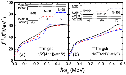
Figure 17: The dependence of the calculated MOIs of the GSBs $\pi 1/2^{+}[411](\alpha=1/2)$ in ¹⁶⁷Tm and ¹⁷¹Tm on the size of neutron shell gaps at $N=98$ and $N=102$. Upper parts of the panels (a) and (b) show the single-particle states at no rotation around these gaps and their modifications discussed in the text. The columns (A) in both panels show these states as obtained in the calculations with no modifications [see Fig. 11(b)]. The columns (B) and (C) in panel (a) show the cases when the neutron orbital $\nu 5/2^{+}[642]$ is shifted up in energy by 0.04 and 0.08$\hbar\omega_{0}$, respectively. In the panel (b), the situations corresponding to the shift up in energy of the neutron $\nu 5/2^{-}$[512] orbital by 0.03 and 0.06$\hbar\omega_{0}$ are illustrated in the columns (B) and (C), respectively.

In Fig. 17 the dependence of the MOIs of selected bands on the size of neutron gaps at $N=98$ and $N=102$ is shown with the goal to evaluate the effects of shell gap sizes on band crossing features. In Fig. 17(a), the neutron orbital $\nu 5/2^{+}[642]$ in ¹⁶⁷Tm is shifted up in energy by 0.04 and 0.08$\hbar\omega_{0}$ to make the $N=98$ gap smaller [see Fig. 11(b)]. Note that $\hbar\omega_{0}$ is the harmonic oscillator frequency in Eq. (II.4). For the latter value, the upbend in ¹⁶⁷Tm is significantly sharper as compared with the cases obtained for the 0.04$\hbar\omega_{0}$ shift of the $\nu 5/2^{+}[642]$ orbital and the original size of the $N=98$ gap. In Fig. 17(b), the neutron $\nu 5/2^{-}$[512] orbital in ¹⁷¹Tm is shifted up in energy by 0.03 and 0.06$\hbar\omega_{0}$ to make the $N=102$ gap larger. It can be seen that with the $N=102$ gap increasing, smooth upbending in ¹⁷¹Tm gets washed out. There is no $N=102$ gap in our calculations without above mentioned modifications. It was suggested in Ref. Asgar et al. (2017) that this may lead to a sharp backbending. However, present calculations do not show even sharp upbend. Thus, one can conclude that the $N=102$ gap has a smaller influence on the alignment features as compared with the $N=98$ gap.

With increasing neutron number $N$ the neutron Fermi level moves from the vicinity of the $\nu 5/2^{+}[642]$ orbital towards the $\nu 7/2^{+}[633]$ orbital. However, the gradual alignment of the latter orbital is not affected by the size of the $N=102$ gap. Thus, the present calculations show that no matter whether the $N=102$ gap exists or not, the alignment is much more gradual in ¹⁷¹Tm as compared with ¹⁶⁷Tm in which upbending is clearly visible. Therefore, this has confirmed our previous conclusion that the band crossing features not only depends on the shell structure close to the Fermi level, but also on specific high-$j$ orbital located in the vicinity of this surface.

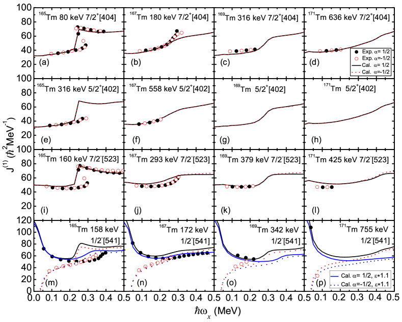
Figure 18: The experimental and calculated MOIs $J^{(1)}$ for excited 1-qp bands in ^{165,167,169,171}Tm. The experimental MOIs are displayed by black solid and red open circles for the $\alpha=+1/2$ and $\alpha=-1/2$ branches of rotational band, respectively. Corresponding calculated values are shown by black solid ($\alpha=+1/2$) and red dotted ($\alpha=-1/2$) lines. The experimental data are taken from Refs. Jain et al. (2006); Baglin (2000, 2008b); Baglin and McCutchan (2018). The experimental excitation energies of the bandheads of rotational bands are also displayed. Solid and dotted blue lines are used in bottom panels for the results of the calculations obtained with quadrupole deformation increased by 10%.

There are significant number of 1-qp excited rotational bands observed in ^{165,167,169,171}Tm. Fig. 18 shows experimental and calculated MOIs for these bands. With few exceptions, the PNC-CSM calculations reproduce their MOIs well. For example, the PNC-CSM calculations somewhat overestimate the MOIs of the $\pi 7/2^{-}$[523] bands in ^167,171Tm [see Figs. 18(j) and (l)]. In addition, the calculations predict a sharp upbending instead of backbending seen in experiment in the $\pi 7/2^{+}[404]$ and $\pi 7/2^{-}[523]$ bands of ¹⁶⁵Tm [see Figs. 18(a) and (i)]. Similar upbending is predicted also in the $\pi 5/2^{+}[402]$ band of ¹⁶⁵Tm but it is not seen in experiment [see Fig. 18(e)].

In a given nucleus, neutron configurations of the 1-qp bands are the same because the equilibrium deformations are the same for all bands in the calculations. As a consequence, neutron MOIs and calculated neutron backbending/upbending are the same for all bands; the minor differences between calculated curves seen in panels (a,e,i), (b,f,j), (c,g,k) and (d,h,l) of Fig. 18 are due to odd proton state. The systematics of experimental data in this mass region shows that with exception of the $\pi 1/2^{-}$[541] band the backbending/upbendings frequencies for all 1-qp rotational bands in a given nucleus are very close to each other. In the $\pi 1/2^{-}$[541] bands the upbending takes place in experiment at higher frequency as compared with other bands [see Fig. 18(m)] or is even absent [see Fig. 18(n)].

Delayed crossing frequency in the $\pi 1/2^{-}$[541] band is explained by strong prolate deformation driving effect of underlying single-particle orbital; this effect has been confirmed both in experiment and in the calculations Nazarewicz et al. (1990); Warburton et al. (1995). Indeed, the PNC-CSM calculations with the deformation which is the same as for other bands fail to reproduce experimental band crossing features [see Figs. 18(m) and (n)]. However, the increase of the quadrupole deformations $\varepsilon_{2}$ of all $\pi 1/2^{-}[541]$ bands by 10% leads to a substantial improvement of the description of experimental situation [see Figs. 18(m), (n) and (o)]. With this modification, the MOIs of the $\pi 1/2^{-}$[541] bands in ^167,169Tm can be reproduced rather well. However, the experimental frequency of upbending in the $\alpha=1/2$ branch of the $1/2^{-}[541]$ band in ¹⁶⁵Tm is still underestimated in the calculations.

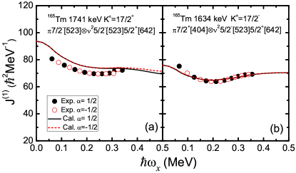
Figure 19: The experimental and calculated MOIs $J^{(1)}$ of two 3-qp bands in ¹⁶⁵Tm with $K^{\pi}=17/2^{+}$ (a) and $K^{\pi}=17/2^{-}$ (b). The experimental data are taken from Ref. Jensen et al. (2001).

Figure 19 shows experimental and calculated MOIs of two 3-qp bands observed in ¹⁶⁵Tm with the structure $K^{\pi}=17/2^{+}$ ($\pi 7/2^{-}[523]\otimes\nu^{2}5/2^{+}[642]5/2^{-}[523]$) and $K^{\pi}=17/2^{-}$ ($\pi 7/2^{+}[404]\otimes\nu^{2}5/2^{+}[642]5/2^{-}[523]$). The MOIs of the $K^{\pi}=17/2^{-}$ band are reproduced rather well. On the contrary, the calculated MOIs for the $K^{\pi}=17/2^{+}$ band are larger than experimental data due to the overestimation of MOIs in the $\pi 7/2^{-}$[523] band of this nucleus. The latter feature is present in all Tm isotopes under study with exception of ¹⁶⁹Tm and it may be caused by the configuration dependent deformation effects.

VI Conclusions 

A comparative study of three theoretical approaches, namely, the CRHB+LN approach, the cranking CDFT-SLAP and PNC-CSM, for the description of rotational properties has been performed using the set of even-even and odd-$Z$ rare-earth nuclei as a testing ground. These three models reproduce experimental MOIs (including the evolution of MOIs with rotational frequency and band crossing features) reasonably well for most of the cases but their predictions at rotational frequencies above the first band crossing can differ substantially.

The comparison of these models in the case of even-even nuclei reveals the following features:

1. There are no free parameters in the particle-hole channel of the CDFT-based models. The calculated results obtained with different CEDFs within the framework of one model are in general close to each other. The results of the CRHB+LN and the cranking CDFT-SLAP calculations are typically closer to each other than to those obtained with PNC-CSM. Note that CDFT+LN is based on fully variational approach, while cranking CDFT-SLAP employs shell model approach.

2. At present, the strength of pairing correlations is adjusted to experimental data at low spin in the CDFT-based models. The need for that is dictated by the lack of global studies of pairing in the CDFT. For example, the requirement for the variation of the strength of the Gogny pairing with particle number in the RHB, CRHB and CRHB+LN approaches is known for some time Afanasjev et al. (2003); Wang et al. (2013); Agbemava et al. (2014). However, the precise form of this variation has not been established till now. The work in that direction is in progress and there is a hope that its better definition will allow to perform parameter free calculations of rotational properties across the nuclear chart in the future. Similar situation exists also in the cranking CDFT-SLAP in which the monopole pairing is used. The implementation of separable pairing of Ref. Tian et al. (2009) into this framework and subsequent study of particle number dependencies of separable pairing across the nuclear chart will allow to improve the predictive power of the model. Note that the pairing gaps obtained with the Gogny and separable pairings are closely correlated and show the same particle number dependencies Agbemava et al. (2014).

3. The models differ in the treatment of particle number. In the cranking CDFT-SLAP, the particle number is totally conserved from beginning to the end and the Pauli blocking effects are taken into account exactly. By iterating the occupation probabilities of single-particle levels back to the densities and currents, cranking CDFT-SLAP is fully self-consistent. Due to exact particle number conservation, there is no pairing collapse even at very high spins. On the contrary, an approximate particle number projection by means of the LN method is employed in the CRHB+LN approach. However, the comparison of the results of the calculations within the cranking CDFT-SLAP and CRHB+LN approaches indicates that the LN method is a reasonable and practical approximation to exact particle number projection. It allows to avoid the pairing collapse for most of the cases in the frequency range of interest making the CRHB+LN approach suitable for the description of yrast bands in even-even systems.

4. However, there are some technical limitations in both CDFT-based models. In the CRHB+LN approach, there is no numerical convergence in some cases in the vicinity of second band crossings and at extremely high rotational frequencies. The former numerical instability is most likely caused by the competition of different configurations located at comparable energies in the region of second band crossing. The latter one is most likely connected with the pairing collapse but it typically takes place when the additional binding due to pairing is in the range of several tens of keV. At these high rotational frequencies the calculations without pairing in the CRMF framework (see Ref. Vretenar et al. (2005) and references quoted therein) represent a feasible alternative to the CRHB+LN ones and such calculations are significantly more numerically stable. In the cranking CDFT-SLAP calculations, minor staggering of MOIs and pairing energies as a function of rotational frequency is observed in some frequency ranges. This appears for the situations of high level density of the single-particle states in the vicinity of the Fermi level leading to competing minima corresponding to slightly different MPCs with relatively small energy differences. To avoid this staggering in calculated quantities the MPCs have to be traced as a function of rotational frequency by using single-particle level tracking technique. However, this is extremely time consuming for systematic investigations of heavy nuclei.

5. The PNC-CSM is built on phenomenological Nilsson potential and employs the same treatment of pairing correlations as in cranking CDFT-SLAP. This model is non-selfconsistent since the Nilsson parameters ($\kappa,\mu$) are fitted to experimental data on single-particle states and deformation parameters ($\varepsilon_{2},\varepsilon_{4}$) are defined from other model (such as microscopic+macroscopic model). Therefore, the predictive power (especially in the extrapolations to other nuclei/regions) is lower than in the CDFT-based methods. In addition, the PNC-CSM uses fixed deformation defined from the ground state results. Thus, this approach faces the difficulties when the shape of nucleus depends on the configuration (as in the case of strongly deformation driving orbital $\pi 1/2^{-}[541]$ in odd-mass nuclei) or when the deformation changes with angular momentum Simpson et al. (1984); Simons et al. (2003).

6. However, there are some important practical benefits of the PNC-CSM. Its computational cost is significantly smaller as compared with CDFT-based models and numerical calculations of odd-$A$ and even-even nuclei require similar computational efforts (contrary to the CDFT-based approaches which require significantly larger computational efforts in odd-mass nuclei as compared with even-even ones). With the Nilsson parameters ($\kappa,\mu$) fitted to experimental data on single-particle energies, it has substantially better spectroscopic properties as compared with CEDFs, and thus, in general, is expected to provide a better descriptive power in odd-mass nuclei.

7. The CDFT-based models predict sharper band crossing features as compared with PNC-CSM calculations. This is caused by the change of the mean fields and corresponding single-particle level structures at the band crossing which leads to a weak interaction of the GSB and $s$-band. In a few cases, predicted sharp upbendings contradict to experimental data. On the contrary, the PNC-CSM predicts gradual upbendings in many cases, which is a consequence of fixed deformation used in the calculations, but there again are the cases contradicting to experiment. A possible way to improve the description of band crossing features would be to use the angular momentum projection technique instead of the cranking method. However, as illustrated by numerous examples obtained in projected shell model that does not necessary resolve all cases of the discrepancies between theory and experiment Wu et al. (2017). Note that a fully self-consistent mean field method with angular momentum projection, configuration mixing and exact particle-number conservation would be extremely time-consuming.

As illustrated by few examples, the calculations of rotational properties in odd-mass nuclei are very time-consuming in the cranking CDFT-SLAP and CRHB+LN approaches and they face a number of technical difficulties. Thus, the systematic investigation of such properties in odd-$A$ ^{165,167,169,171}Tm nuclei has been performed only in the PNC-CSM. In these calculations, with few exceptions the evolutions of the MOIs of the 1-qp and 3-qp bands with rotational frequency (including backbending/upbending regions) as well as their changes with neutron number are reproduced reasonably well. By analyzing the occupation probabilities of the Nilsson orbitals located in the vicinity of the Fermi level and the contributions of each major shell to the angular momentum alignments, the origin and the evolution of the backbendings/upbendings with neutron number in these nuclei are clearly understood. The impact of the shell gap size on the band crossing features is also investigated. In the PNC-CSM calculations, the band crossing features depend not only on the shell structure in the vicinity of the Fermi level but also on specific high-$j$ orbital.

VII Acknowledgement

Helpful discussions with Z. Shi and B. W. Xiong are gratefully acknowledged. This work is supported by National Natural Science Foundation of China (11875027, 11775112, 11775026, 11775099), Fundamental Research Funds for the Central Universities (2018MS058), the program of China Scholarships Council (No. 201850735020) and the U.S. Department of Energy, Office of Science, Office of Nuclear Physics under Award No. DE-SC0013037.

References

- Johnson et al. (1971) A. Johnson, H. Ryde, and J. Sztarkier, Phys. Lett. B 34, 605 (1971).
- Lee et al. (1977) I. Y. Lee, M. M. Aleonard, M. A. Deleplanque, Y. El-Masri, J. O. Newton, R. S. Simon, R. M. Diamond, and F. S. Stephens, Phys. Rev. Lett. 38, 1454 (1977).
- Bengtsson and Ragnarsson (1983) T. Bengtsson and I. Ragnarsson, Phys. Scr. T5, 165 (1983).
- Afanasjev et al. (1999a) A. Afanasjev, D. Fossan, G. Lane, and I. Ragnarsson, Phys. Rep. 322, 1 (1999a).
- Bengtsson et al. (1984) R. Bengtsson, H. Frisk, F. R. May, and J. A. Pinston, Nucl. Phys. A 415, 189 (1984).
- Twin et al. (1986) P. J. Twin, B. M. Nyakó, A. H. Nelson, J. Simpson, M. A. Bentley, H. W. Cranmer-Gordon, P. D. Forsyth, D. Howe, A. R. Mokhtar, J. D. Morrison, J. F. Sharpey-Schafer, and G. Sletten, Phys. Rev. Lett. 57, 811 (1986).
- Ødegård et al. (2001) S. W. Ødegård, G. B. Hagemann, D. R. Jensen, M. Bergström, B. Herskind, G. Sletten, S. Törmänen, J. N. Wilson, P. O. Tjøm, I. Hamamoto, K. Spohr, H. Hübel, A. Görgen, G. Schönwasser, A. Bracco, S. Leoni, A. Maj, C. M. Petrache, P. Bednarczyk, and D. Curien, Phys. Rev. Lett. 86, 5866 (2001).
- Stephens and Simon (1972) F. S. Stephens and R. S. Simon, Nucl. Phys. A 183, 257 (1972).
- de Voigt et al. (1983) M. J. A. de Voigt, J. Dudek, and Z. Szymański, Rev. Mod. Phys. 55, 949 (1983).
- Szymański (1983) Z. Szymański, Fast Nuclear Rotation (Clarendon Press, 1983).
- Asgar et al. (2017) M. A. Asgar, T. Roy, G. Mukherjee, A. Dhal, S. Bhattacharya, S. Bhattacharyya, C. Bhattacharya, S. Bhattacharya, A. Chaudhuri, K. Banerjee, S. Kundu, S. Manna, R. Pandey, J. K. Meena, R. Palit, S. Biswas, S. Saha, J. Sethi, P. Singh, and D. Choudhury, Phys. Rev. C 95, 031304R (2017).
- Jensen et al. (2001) H. J. Jensen, R. A. Bark, P. O. Tjøm, G. B. Hagemann, I. G. Bearden, H. Carlsson, S. Leoni, T. Lönnroth, W. Reviol, L. L. Riedinger, H. Schnack-Petersen, T. Shizuma, X. Z. Wang, and J. Wrzesinski, Nucl. Phys. A 695, 3 (2001).
- Burns et al. (2005) M. J. Burns, R. Chapman, K. M. Spohr, J. Ollier, M. Labiche, X. Liang, E. Farnea, M. Axiotis, T. Martinez, D. R. Napoli, C. A. Ur, and T. Kröll, J. Phys. G: Nucl. Part. Phys. 31, S1827 (2005).
- Bengtsson et al. (1978) R. Bengtsson, I. Hamamoto, and B. Mottelson, Phys. Lett. B 73, 259 (1978).
- Wu and Zeng (1991a) C. S. Wu and J. Y. Zeng, Phys. Rev. Lett. 66, 1022 (1991a).
- Andersson et al. (1976) G. Andersson, S. E. Larsson, G. Leander, P. Möller, S. G. Nilsson, I. Ragnarsson, S. Åberg, R. Bengtsson, J. Dudek, B. Nerlo-Pomorska, K. Pomorski, and Z. Szymanski, Nucl. Phys. A 268, 205 (1976).
- Bengtsson and Frauendorf (1979) R. Bengtsson and S. Frauendorf, Nucl. Phys. A 327, 139 (1979).
- Nazarewicz et al. (1985) W. Nazarewicz, J. Dudek, R. Bengtsson, T. Bengtsson, and I. Ragnarsson, Nucl. Phys. A 435, 397 (1985).
- Ćwiok et al. (1987) S. Ćwiok, J. Dudek, W. Nazarewicz, J. Skalski, and T. Werner, Comput. Phys. Commun. 46, 379 (1987).
- Hara and Sun (1995) H. Hara and Y. Sun, Int. J. Mod. Phys. E 4, 637 (1995).
- Frauendorf (2001) S. Frauendorf, Rev. Mod. Phys. 73, 463 (2001).
- Afanasjev et al. (1996) A. V. Afanasjev, J. König, and P. Ring, Nucl. Phys. A 608, 107 (1996).
- Afanasjev et al. (2000a) A. V. Afanasjev, J. König, P. Ring, L. M. Robledo, and J. L. Egido, Phys. Rev. C 62, 054306 (2000a).
- Terasaki et al. (1995) J. Terasaki, P. H. Heenen, P. Bonche, J. Dobaczewski, and H. Flocard, Nucl. Phys. A 593, 1 (1995).
- Egido and Robledo (1993) J. L. Egido and L. M. Robledo, Phys. Rev. Lett. 70, 2876 (1993).
- Afanasjev et al. (2000b) A. V. Afanasjev, P. Ring, and J. König, Nucl. Phys. A 676, 196 (2000b).
- Shi et al. (2018) Z. Shi, Z. H. Zhang, Q. B. Chen, S. Q. Zhang, and J. Meng, Phys. Rev. C 97, 034317 (2018).
- Zeng et al. (1994a) J. Y. Zeng, T. H. Jin, and Z. J. Zhao, Phys. Rev. C 50, 1388 (1994a).
- Ring (1996) P. Ring, Prog. Part. Nucl. Phys. 37, 193 (1996).
- Vretenar et al. (2005) D. Vretenar, A. Afanasjev, G. Lalazissis, and P. Ring, Phys. Rep. 409, 101 (2005).
- Meng et al. (2006a) J. Meng, H. Toki, S. Zhou, S. Zhang, W. Long, and L. Geng, Prog. Part. Nucl. Phys. 57, 470 (2006a).
- Lal (2004) Extended Density Functionals in Nuclear Structure Physics, Vol. 641 of Lecture Notes in Physics, edited by G. A. Lalazissis, P. Ring and D. Vretenar (Springer-Verlag, Heidelberg, 2004).
- Cohen et al. (1992) T. D. Cohen, R. J. Furnstahl, and D. K. Griegel, Phys. Rev. C 45, 1881 (1992).
- Bender et al. (1999) M. Bender, K. Rutz, P.-G. Reinhard, J. A. Maruhn, and W. Greiner, Phys. Rev. C 60, 034304 (1999).
- Litvinova and Afanasjev (2011) E. V. Litvinova and A. V. Afanasjev, Phys. Rev. C 84, 014305 (2011).
- Afanasjev and Abusara (2010a) A. V. Afanasjev and H. Abusara, Phys. Rev. C 81, 014309 (2010a).
- Afanasjev and Ring (2000) A. V. Afanasjev and P. Ring, Phys. Rev. C 62, 031302(R) (2000).
- Meng et al. (2013) J. Meng, J. Peng, S.-Q. Zhang, and P.-W. Zhao, Frontiers Phys. 8, 55 (2013).
- König and Ring (1993) J. König and P. Ring, Phys. Rev. Lett. 71, 3079 (1993).
- Madokoro et al. (2000) H. Madokoro, J. Meng, M. Matsuzaki, and S. Yamaji, Phys. Rev. C 62, 061301R (2000).
- Peng et al. (2008) J. Peng, J. Meng, P. Ring, and S. Q. Zhang, Phys. Rev. C 78, 024313 (2008).
- Zhao et al. (2011a) P. W. Zhao, S. Q. Zhang, J. Peng, H. Z. Liang, P. Ring, and J. Meng, Phys. Lett. B 699, 181 (2011a).
- Zhao et al. (2015a) P. W. Zhao, S. Q. Zhang, and J. Meng, Phys. Rev. C 92, 034319 (2015a).
- Zhao et al. (2011b) P. W. Zhao, J. Peng, H. Z. Liang, P. Ring, and J. Meng, Phys. Rev. Lett. 107, 122501 (2011b).
- Zhao et al. (2012) P. W. Zhao, J. Peng, H. Z. Liang, P. Ring, and J. Meng, Phys. Rev. C 85, 054310 (2012).
- Liu (2019) L. Liu, Phys. Rev. C 99, 024317 (2019).
- Zhao (2017) P. Zhao, Phys. Lett. B 773, 1 (2017).
- Zhao et al. (2015b) P. W. Zhao, N. Itagaki, and J. Meng, Phys. Rev. Lett. 115, 022501 (2015b).
- Zhao and Li (2018) P. Zhao and Z. Li, Int. J. Mod. Phys. E 27, 1830007 (2018).
- Afanasjev and Abusara (2018) A. V. Afanasjev and H. Abusara, Phys. Rev. C 97, 024329 (2018).
- Ren et al. (2019) Z. X. Ren, S. Q. Zhang, P. W. Zhao, N. Itagaki, J. A. Maruhn, and J. Meng, Sci. China-Phys. Mech. Astron. 62, 112062 (2019).
- Afanasjev et al. (2019) A. V. Afanasjev, N. Itagaki, and D. Ray, Phys. Lett. B 794, 7 (2019).
- Nilsson (1955) S. G. Nilsson, Dan. Mat. Fys. Medd. 29, No.16 (1955).
- Nilsson et al. (1969) S. G. Nilsson, C. F. Tsang, A. Sobiczewski, Z. Szymański, S. Wycech, C. Gustafson, I. L. Lamm, P. Möller, and B. Nilsson, Nucl. Phys. A 131, 1 (1969).
- Nilsson and Ragnarsson (1995) S. G. Nilsson and I. Ragnarsson, Shapes and Shells in Nuclear Structure (Cambridge University Press, Cambridge, 1995).
- Petrache et al. (2019) C. M. Petrache, S. Frauendorf, B. F. Lv, A. Astier, E. Dupont, S. Guo, M. L. Liu, X. H. Zhou, K. L. Wang, P. T. Greenlees, H. Badran, D. M. Cox, T. Grahn, R. Julin, S. Juutinen, J. Konki, J. Pakarinen, P. Papadakis, J. Partanen, P. Rahkila, M. Sandzelius, J. Saren, C. Scholey, J. Sorri, S. Stolze, J. Uusitalo, B. Cederwall, O. Aktas, A. Ertoprak, H. Liu, I. Kuti, J. Timár, A. Tucholski, J. Srebrny, and C. Andreoiu, Phys. Rev. C 99, 041301(R) (2019).
- Bhattacharya et al. (2019) S. Bhattacharya, T. Trivedi, D. Negi, R. P. Singh, S. Muralithar, R. Palit, I. Ragnarsson, S. Nag, S. Rajbanshi, M. K. Raju, V. V. Parkar, G. Mohanto, S. Kumar, D. Choudhury, R. Kumar, R. K. Bhowmik, S. C. Pancholi, and A. K. Jain, Phys. Rev. C 100, 014315 (2019).
- Bohr and Mottelson (1975) A. Bohr and B. R. Mottelson, Nuclear Structure, Vol. II Nuclear Deformation (Benjamin, New York, 1975).
- Ring and Schuck (1980) P. Ring and P. Schuck, The Nuclear Many-Body Problem (Springer-Verlag, 1980).
- Meng (2015) J. Meng, Relativistic Density Functional for Nuclear Structure (World Scientific, Singapore, 2015).
- Mottelson and Valatin (1960) B. R. Mottelson and J. G. Valatin, Phys. Rev. Lett. 5, 511 (1960).
- Sano and Wakai (1972) M. Sano and M. Wakai, Prog. Theo. Phys. 48, 160 (1972).
- Lipkin (1960) H. J. Lipkin, Ann. Phys. 9, 272 (1960).
- Lipkin (1961) H. J. Lipkin, Ann. Phys. 12, 452 (1961).
- Nogami (1964) Y. Nogami, Phys. Rev. 134, B313 (1964).
- Gall et al. (1994) B. Gall, P. Bonche, J. Dobaczewski, H. Flocard, and P.-H. Heenen, Z. Phys. A 348, 183 (1994).
- Valor et al. (1996) A. Valor, J. L. Egido, and L. M. Robledo, Phys. Rev. C 53, 172 (1996).
- Afanasjev et al. (1999b) A. V. Afanasjev, J. König, and P. Ring, Phys. Rev. C 60, 051303 (1999b).
- O’Leary et al. (2003) C. D. O’Leary, C. E. Svensson, S. G. Frauendorf, A. V. Afanasjev, D. E. Appelbe, R. A. E. Austin, G. C. Ball, J. A. Cameron, R. M. Clark, M. Cromaz, P. Fallon, D. F. Hodgson, N. S. Kelsall, A. O. Macchiavelli, I. Ragnarsson, D. Sarantites, J. C. Waddington, and R. Wadsworth, Phys. Rev. C 67, 021301(R) (2003).
- Afanasjev and Abdurazakov (2013) A. V. Afanasjev and O. Abdurazakov, Phys. Rev. C 88, 014320 (2013).
- Afanasjev (2014) A. V. Afanasjev, Phys. Scr. 89, 054001 (2014).
- Jeppesen et al. (2009) H. B. Jeppesen, R. M. Clark, K. E. Gregorich, A. V. Afanasjev, M. N. Ali, J. M. Allmond, C. W. Beausang, M. Cromaz, M. A. Deleplanque, I. Dragojević, J. Dvorak, P. A. Ellison, P. Fallon, M. A. Garcia, J. M. Gates, S. Gros, I. Y. Lee, A. O. Macchiavelli, S. L. Nelson, H. Nitsche, L. Stavsetra, F. S. Stephens, and M. Wiedeking, Phys. Rev. C 80, 034324 (2009).
- Herzberg et al. (2009) R. Herzberg, S. Moon, S. Eeckhaudt, P. Greenlees, P. Butler, T. Page, A. Afanasjev, N. Amzal, J. Bastin, F. Becker, M. Bender, B. Bruyneel, J. Cocks, I. Darby, O. Dorvaux, K. Eskola, J. Gerl, T. Grahn, C. Gray-Jones, N. Hammond, K. Hauschild, P. Heenen, K. Helariutta, A. Herzberg, F. Hessberger, M. Houry, A. Hürstel, R. Humphreys, G. Jones, P. Jones, R. Julin, S. Juutinen, H. Kankaanpȧȧ, H. Kettunen, T. Khoo, W. Korten, P. Kuusiniemi, Y. LeCoz, M. Leino, A. Leppȧnen, C. Lister, R. Lucas, M. Muikku, P. Nieminen, M. Nyman, R. Page, T. Page, J. Pakarinen, A. Pritchard, P. Rahkila, P. Reiter, M. Sandzelius, J. Saren, C. Schlegel, C. Scholey, C. Theisen, W. Trzaska, J. Uusitalo, A. Wiens, and H. Wollersheim, Eur. Phys. J. A 42, 333 (2009).
- Afanasjev and Frauendorf (2005) A. V. Afanasjev and S. Frauendorf, Phys. Rev. C 71, 064318 (2005).
- Ray and Afanasjev (2016) D. Ray and A. V. Afanasjev, Phys. Rev. C 94, 014310 (2016).
- Andreoiu et al. (2007) C. Andreoiu, C. E. Svensson, A. V. Afanasjev, R. A. E. Austin, M. P. Carpenter, D. Dashdorj, P. Finlay, S. J. Freeman, P. E. Garrett, J. Greene, G. F. Grinyer, A. Görgen, B. Hyland, D. Jenkins, F. Johnston-Theasby, P. Joshi, A. O. Machiavelli, F. Moore, G. Mukherjee, A. A. Phillips, W. Reviol, D. G. Sarantites, M. A. Schumaker, D. Seweryniak, M. B. Smith, J. J. Valiente-Dobón, and R. Wadsworth, Phys. Rev. C 75, 041301(R) (2007).
- Davies et al. (2007) P. J. Davies, A. V. Afanasjev, R. Wadsworth, C. Andreoiu, R. A. E. Austin, M. P. Carpenter, D. Dashdorj, S. J. Freeman, P. E. Garrett, A. Görgen, J. Greene, D. G. Jenkins, F. L. Johnston-Theasby, P. Joshi, A. O. Macchiavelli, F. Moore, G. Mukherjee, W. Reviol, D. Sarantites, D. Seweryniak, M. B. Smith, C. E. Svensson, J. J. Valiente-Dobon, and D. Ward, Phys. Rev. C 75, 011302(R) (2007).
- Dobaczewski and Nazarewicz (1993) J. Dobaczewski and W. Nazarewicz, Phys. Rev. C 47, 2418 (1993).
- Sheikh et al. (2002) J. A. Sheikh, P. Ring, E. Lopes, and R. Rossignoli, Phys. Rev. C 66, 044318 (2002).
- Egido and Ring (1982) J. Egido and P. Ring, Nucl. Phys. A 388, 19 (1982).
- Anguiano et al. (2001) M. Anguiano, J. Egido, and L. Robledo, Nucl. Phys. A 696, 467 (2001).
- Volya et al. (2001) A. Volya, B. A. Brown, and V. Zelevinsky, Phys. Lett. B 509, 37 (2001).
- Stoitsov et al. (2007) M. V. Stoitsov, J. Dobaczewski, R. Kirchner, W. Nazarewicz, and J. Terasaki, Phys. Rev. C 76, 014308 (2007).
- Bender et al. (2009) M. Bender, T. Duguet, and D. Lacroix, Phys. Rev. C 79, 044319 (2009).
- Yao et al. (2014) J. M. Yao, K. Hagino, Z. P. Li, J. Meng, and P. Ring, Phys. Rev. C 89, 054306 (2014).
- Zeng and Cheng (1983) J. Y. Zeng and T. S. Cheng, Nucl. Phys. A 405, 1 (1983).
- Pillet et al. (2002) N. Pillet, P. Quentin, and J. Libert, Nucl. Phys. A 697, 141 (2002).
- Meng et al. (2006b) J. Meng, J.-Y. Guo, L. Liu, and S.-Q. Zhang, Front. Phys. China 1, 38 (2006b).
- Wu and Zeng (1989) C. S. Wu and J. Y. Zeng, Phys. Rev. C 39, 666 (1989).
- Molique and Dudek (1997) H. Molique and J. Dudek, Phys. Rev. C 56, 1795 (1997).
- Fu et al. (2013) X. M. Fu, F. R. Xu, J. C. Pei, C. F. Jiao, Y. Shi, Z. H. Zhang, and Y. A. Lei, Phys. Rev. C 87, 044319 (2013).
- Liang et al. (2015) W. Y. Liang, C. F. Jiao, Q. Wu, X. M. Fu, and F. R. Xu, Phys. Rev. C 92, 064325 (2015).
- Zeng et al. (1994b) J. Y. Zeng, Y. A. Lei, T. H. Jin, and Z. J. Zhao, Phys. Rev. C 50, 746 (1994b).
- Zeng et al. (2001) J. Y. Zeng, S. X. Liu, Y. A. Lei, and L. Yu, Phys. Rev. C 63, 024305 (2001).
- Liu et al. (2002) S. X. Liu, J. Y. Zeng, and E. G. Zhao, Phys. Rev. C 66, 024320 (2002).
- Wu et al. (2011) X. Wu, Z. H. Zhang, J. Y. Zeng, and Y. A. Lei, Phys. Rev. C 83, 034323 (2011).
- Zhang et al. (2013a) Z.-H. Zhang, P.-W. Zhao, J. Meng, J.-Y. Zeng, E.-G. Zhao, and S.-G. Zhou, Phys. Rev. C 87, 054314 (2013a).
- Zhang (2016) Z.-H. Zhang, Phys. Rev. C 94, 034305 (2016).
- Zhang (2019) Z.-H. Zhang, Chin. Phys. C 43, 054107 (2019).
- Zhang et al. (2009) Z. H. Zhang, Y. A. Lei, and J. Y. Zeng, Phys. Rev. C 80, 034313 (2009).
- Zhang (2018) Z.-H. Zhang, Phys. Rev. C 98, 034304 (2018).
- He and Li (2018) X.-T. He and Y.-C. Li, Phys. Rev. C 98, 064314 (2018).
- Liu et al. (2019) S.-Y. Liu, M. Huang, and Z.-H. Zhang, Phys. Rev. C 100, 064307 (2019).
- Dai and Xu (2019) A. C. Dai and F. R. Xu, Chin. Sci. Bull. 64 (2019), 10.1360/TB-2019-0044.
- He et al. (2009) X. T. He, Z. Z. Ren, S. X. Liu, and E. G. Zhao, Nucl. Phys. A 817, 45 (2009).
- Zhang et al. (2011) Z.-H. Zhang, J.-Y. Zeng, E.-G. Zhao, and S.-G. Zhou, Phys. Rev. C 83, 011304R (2011).
- Zhang et al. (2012) Z.-H. Zhang, X.-T. He, J.-Y. Zeng, E.-G. Zhao, and S.-G. Zhou, Phys. Rev. C 85, 014324 (2012).
- Zhang et al. (2013b) Z.-H. Zhang, J. Meng, E.-G. Zhao, and S.-G. Zhou, Phys. Rev. C 87, 054308 (2013b).
- Fu et al. (2014) X. M. Fu, F. R. Xu, C. F. Jiao, W. Y. Liang, J. C. Pei, and H. L. Liu, Phys. Rev. C 89, 054301 (2014).
- Richardson and Sherman (1964) R. Richardson and N. Sherman, Nucl. Phys. 52, 221 (1964).
- Pan et al. (1998) F. Pan, J. Draayer, and W. Ormand, Phys. Lett. B 422, 1 (1998).
- Jia (2013a) L. Y. Jia, Phys. Rev. C 88, 044303 (2013a).
- Jia (2013b) L. Y. Jia, Phys. Rev. C 88, 064321 (2013b).
- Chen et al. (2014) W.-C. Chen, J. Piekarewicz, and A. Volya, Phys. Rev. C 89, 014321 (2014).
- Xiong (2019) B. Xiong, arXiv: 1908.03561 (2019).
- Tian et al. (2009) Y. Tian, Z. Ma, and P. Ring, Phys. Lett. B 676, 44 (2009).
- Berger et al. (1991) J. F. Berger, M. Girod, and D. Gogny, Comput. Phys. Commun. 63, 365 (1991).
- Agbemava et al. (2014) S. E. Agbemava, A. V. Afanasjev, D. Ray, and P. Ring, Phys. Rev. C 89, 054320 (2014).
- Boguta and Bodmer (1977) J. Boguta and A. Bodmer, Nucl. Phys. A 292, 413 (1977).
- Gambhir et al. (1990) Y. K. Gambhir, P. Ring, and A. Thimet, Ann. Phys. 198, 132 (1990).
- Reinhard et al. (1986) P. G. Reinhard, M. Rufa, J. Maruhn, W. Greiner, and J. Friedrich, Z. Phys. A 323, 13 (1986).
- Agbemava et al. (2019) S. E. Agbemava, A. V. Afanasjev, and A. Taninah, Phys. Rev. C 99, 014318 (2019).
- Roca-Maza et al. (2011) X. Roca-Maza, X. Viñas, M. Centelles, P. Ring, and P. Schuck, Phys. Rev. C 84, 054309 (2011).
- Zhao et al. (2010) P. W. Zhao, Z. P. Li, J. M. Yao, and J. Meng, Phys. Rev. C 82, 054319 (2010).
- Afanasjev et al. (2003) A. V. Afanasjev, T. L. Khoo, S. Frauendorf, G. A. Lalazissis, and I. Ahmad, Phys. Rev. C 67, 024309 (2003).
- Afanasjev and Abusara (2010b) A. V. Afanasjev and H. Abusara, Phys. Rev. C 82, 034329 (2010b).
- Koepf and Ring (1988) W. Koepf and P. Ring, Phys. Lett. B 212, 397 (1988).
- Afanasjev and Shawaqfeh (2011) A. Afanasjev and S. Shawaqfeh, Phys. Lett. B 706, 177 (2011).
- Afanasjev et al. (1999c) A. V. Afanasjev, I. Ragnarsson, and P. Ring, Phys. Rev. C 59, 3166 (1999c).
- Bengtsson et al. (1986) R. Bengtsson, S. Frauendorf, and F. R. May, At. Data Nucl. Data Tables 35, 15 (1986).
- Bengtsson and Ragnarsson (1985) T. Bengtsson and I. Ragnarsson, Nucl. Phys. A 436, 14 (1985).
- Bengtsson (1990) T. Bengtsson, Nucl. Phys. A 512, 124 (1990).
- Diebel (1984) M. Diebel, Nucl. Phys. A 419, 221 (1984).
- Satuła and Wyss (1994) W. Satuła and R. Wyss, Phys. Rev. C 50, 2888 (1994).
- Sakamoto and Kishimoto (1990) H. Sakamoto and T. Kishimoto, Phys. Lett. B 245, 321 (1990).
- Singh and Chen (2018) B. Singh and J. Chen, Nucl. Data Sheets 147, 1 (2018).
- Baglin (2008a) C. M. Baglin, Nucl. Data Sheets 109, 1103 (2008a).
- Baglin (2010) C. M. Baglin, Nucl. Data Sheets 111, 1807 (2010).
- Baglin et al. (2018) C. Baglin, E. McCutchan, S. Basunia, and E. Browne, Nucl. Data Sheets 153, 1 (2018).
- Firestone et al. (1999) R. Firestone, C. M. Baglin, and S. Y. Frank Chu, Table of Isotopes: 1999 Update with CD-ROM (Wiley, New York, 1999).
- Wu and Zeng (1991b) C. S. Wu and J. Y. Zeng, Phys. Rev. C 44, 2566 (1991b).
- Dobaczewski et al. (2015) J. Dobaczewski, A. V. Afanasjev, M. Bender, L. M. Robledo, and Y. Shi, Special Issue on Superheavy Elements, Nucl. Phys. A 944, 388 (2015).
- Meng et al. (2006c) J. Meng, J. Peng, S. Q. Zhang, and S.-G. Zhou, Phys. Rev. C 73, 037303 (2006c).
- Shimizu et al. (1989) Y. R. Shimizu, J. D. Garrett, R. A. Broglia, M. Gallardo, and E. Vigezzi, Rev. Mod. Phys. 61, 131 (1989).
- Bender et al. (2003) M. Bender, P. Bonche, T. Duguet, and P. H. Heenen, Nucl. Phys. A 723, 354 (2003).
- Jain et al. (2006) A. K. Jain, A. Ghosh, and B. Singh, Nucl. Data Sheets 107, 1075 (2006).
- Baglin (2000) C. M. Baglin, Nucl. Data Sheets 90, 431 (2000).
- Baglin (2008b) C. M. Baglin, Nucl. Data Sheets 109, 2033 (2008b).
- Baglin and McCutchan (2018) C. M. Baglin and E. McCutchan, Nucl. Data Sheets 151, 334 (2018).
- Nazarewicz et al. (1990) W. Nazarewicz, M. A. Riley, and J. D. Garrett, Nucl. Phys. A 512, 61 (1990).
- Warburton et al. (1995) S. Warburton, R. Chapman, J. Copnell, F. Lidén, A. Smith, J. Sweeney, D. Thompson, S. Freeman, G. Hagemann, and M. Piiparinen, Nucl. Phys. A 591, 323 (1995).
- Walker et al. (2009) P. M. Walker, R. J. Wood, G. D. Dracoulis, T. Kibédi, R. A. Bark, A. M. Bruce, A. P. Byrne, P. M. Davidson, H. M. El-Masri, G. J. Lane, C. Moon, J. N. Orce, F. M. P. Estevéz, C. Wheldon, and A. N. Wilson, Phys. Rev. C 79, 044321 (2009).
- Wang et al. (2013) L. J. Wang, B. Y. Sun, J. M. Dong, and W. H. Long, Phys. Rev. C 87, 054331 (2013).
- Simpson et al. (1984) J. Simpson, M. A. Riley, J. R. Cresswell, P. D. Forsyth, D. Howe, B. M. Nyakó, J. F. Sharpey-Schafer, J. Bacelar, J. D. Garrett, G. B. Hagemann, B. Herskind, and A. Holm, Phys. Rev. Lett. 53, 648 (1984).
- Simons et al. (2003) A. J. Simons, R. Wadsworth, D. G. Jenkins, R. M. Clark, M. Cromaz, M. A. Deleplanque, R. M. Diamond, P. Fallon, G. J. Lane, I. Y. Lee, A. O. Macchiavelli, F. S. Stephens, C. E. Svensson, K. Vetter, D. Ward, and S. Frauendorf, Phys. Rev. Lett. 91, 162501 (2003).
- Wu et al. (2017) X.-Y. Wu, S. K. Ghorui, L.-J. Wang, Y. Sun, M. Guidry, and P. M. Walker, Phys. Rev. C 95, 064314 (2017).