Dynamical spin excitations of topological Haldane gapped phase in the $S=1$ Heisenberg antiferromagnetic chain with single-ion anisotropy

Abstract

We study the dynamical spin excitations of the one-dimensional $S=1$ Heisenberg antiferromagnetic chain with single-ion anisotropy by using quantum Monte Carlo simulations and stochastic analytic continuation of imaginary-time correlation function. Using the transverse dynamic spin structure factor, we observe the quantum phase transition with a critical point between the topological Haldane gapped phase and the trivial phase. At the quantum critical point, we find a broad continuum characterized by the Tomonaga-Luttinger liquid similar to a $S=1/2$ Heisenberg antiferromagnetic chain. We further identify that the elementary excitations are fractionalized spinons.

I INTRODUCTION

An extensive body of research has been done on the one-dimensional $S=1$ Heisenberg antiferromagnetic chain, which can be traced back to the original work by Haldane Haldane (1983a, b). Here we investigate the spin chain with single-ion anisotropy Lange et al. (2018) and present the quantum phase diagram Albuquerque et al. (2009); Chen et al. (2003); Oitmaa and Hamer (2008) with a Ising-type Néel phase, a Haldane phase and a large-$D$ phase in Fig. 1. The phase transition from the Néel order to the Haldane phase has been studied in detail before Lambert and Sorensen (2019), which is described by conformal field theory with a central charge $c=1/2$ Tzeng and Yang (2008). Thus, we are more interested in the other transition from the Haldane phase to the large-$D$ phase, i.e. a continuous transition. This quantum phase transition is a Gaussian-type transition Hu et al. (2011) described by conformal field theory with a central charge $c=1$ Rao et al. (2014); Boschi et al. (2003). The Haldane gapped phase is now understood as a symmetry-protected topological phase Rao et al. (2016a), while it will undergo a phase transition to a topologically trivial gapped phase, the large-$D$ phase, with increasing the single-ion anisotropy $D$. When $D$ is strong enough, the ground state in the large-$D$ phase is known as the product state with $S^{z}=0$ at each site. A symmetry-protected topological phase cannot be continuously changed into a trivial gapped phase without closing the energy gap Haegeman et al. (2013), so the transition, between the Haldane phase and the large-$D$ phase, is a topological phase transition that possesses a gapless critical point and does not fit into the Landau-Ginzburg-Wilson paradigm Senthil et al. (2004).

The previous research Rahnavard and Brenig (2015) has suggested that a direct transition from the Haldane phase to the trivial phase can occur without accessing a Tomonaga-Luttinger liquid (TLL) critical state in the absence of external magnetic field, which is inaccurate, or rather easy to be neglected. Recently, the TLL phase of the $S=1/2$ chain has been realized experimentally by the rare-earth perovskite $\mathrm{YbAlO}_{3}$ Wu et al. (2019) and exhibited a broad continuum, a signature of fractionalized spinon excitations, as predicted by various theoretical and numerical methods Ma et al. (2018a, 2019, b); Sandvik (2007). This provides strong evidence to identify that the critical point separating the Haldane phase from the trivial phase is a TLL critical state by the spin excitation spectra theoretically and experimentally. The $S=1$ chain with single-ion anisotropy can be realized by ultracold atomic condensates on optical lattices and various compounds with $\mathrm{Ni}^{2+}$ ions, such as $\mathrm{Ni}(\mathrm{C}_{2}\mathrm{H}_{8}\mathrm{N}_{2})_{2}\mathrm{NO}_{2}(\mathrm{ClO}_{4})$ (NENP), $\mathrm{NiCl}_{2}4\mathrm{SC}(\mathrm{NH}_{2})_{2}$ (DTN) and so on Paduan et al. (2004); Regnault et al. (1994); Renard et al. (1987); Zapf et al. (2006). In addition, experimental methods, including inelastic neutron scattering and nuclear magnetic resonance, provide the dynamic probes of these materials Piazza et al. (2015).

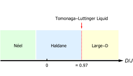
Figure 1: Quantum phase diagram of the $S=1$ Heisenberg chain versus single-ion anisotropy $D/J$. The quantum critical point between the Haldane phase and the large-D phase is a Tomonaga-Luttinger liquid phase (red dashed line).

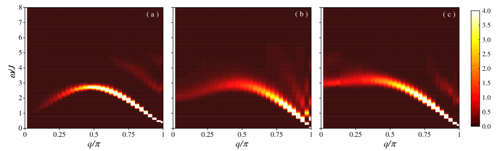
Figure 2: The transverse dynamic spin structure factor $S^{xx}(q,\omega)$ obtained from QMC-SAC calculations for the $S=1$ Heisenberg chain with $L=64$ and $\beta=128$. The values of single-ion anisotropy are (a) $D/J=0$ in the Haldane phase, (b) $D/J=0.97$ in the TLL critical state and (c) $D/J=1.5$ in the large-D phase, respectively.

In this paper, we study the dynamics of the one-dimensional $S=1$ Heisenberg antiferromagnetic chain with single-ion anisotropy Syljuasen (2008). By means of quantum Monte Carlo (QMC) Sandvik (2010, 2002); Henelius et al. (2000); Syljuasen and Sandvik (2002); Bergkvist et al. (2002) simulations and stochastic analytic continuation (SAC), we present and discuss our results for the transverse dynamic spin structure factor. The QMC-SAC numerical methods provided excitation spectra very well in previous studies Huang et al. (2018); Shu et al. (2018); Xu et al. (2019). Here, we study the dynamical spin excitations of the topological Haldane phase and its phase transition to the topologically trivial large-$D$ phase. At the quantum critical point, we show the comparison with the TLL phase of the $S=1/2$ Heisenberg antiferromagnetic chain.

II MODEL AND NUMERICAL METHODS

II.1 Model

We investigate the anisotropic $S=1$ Heisenberg antiferromagnetic chain defined by the Hamiltonian

$$H=\sum_{i}[J(S_{i}^{x}S_{i+1}^{x}+S_{i}^{y}S_{i+1}^{y}+S_{i}^{z}S_{i+1}^{z})+D(S_{i}^{z})^{2}],$$ (1)

where $S_{i}^{x,y,z}$ denotes the $S=1$ spin operator on each site $i$, $J>0$ is the antiferromagnetic exchange, and the parameter $D$ is the single-ion anisotropy. For simplicity, we set $J=1$ in the whole paper.

As shown in Fig. 1, the phase diagram of this model consists of the Néel phase, the Haldane phase, the TLL critical state and the large-$D$ phase. For the isotropic case, i.e. $D/J=0$, the ground state belongs to the symmetry-protected topological Haldane phase with a Haldane gap of $\Delta\approx 0.41J$ White (1992); White and Huse (1993) and the lowest-lying excitations is magnon. Whereas at finite $D$, the magnon excitations will split into a singlet branch ($S^{z}=0$) and a doublet branch ($S^{z}=\pm 1$), which show up in the longitudinal and transverse dynamic spin structure factors respectively Takahashi (1993). In the paper, we are more interested in the phase transition from the Haldane phase to the large-$D$ phase, in which the lowest-lying excitations lie in the $S^{z}=\pm 1$ branch.

II.2 Methods

We numerically solve the model in Eq. (1) by using QMC simulations based on the stochastic series expansion Sandvik (1999); Dorneich and Troyer (2001). Using stochastic analytic continuation of imaginary-time correlation function obtained from QMC simulations, we extract the transverse dynamic spin structure factor $S^{xx}(q,\omega)$, which is written in the basis of eigenstates $\ket{n}$ and eigenvalues $E_{n}$ of the Hamiltonian as

$$S^{xx}(q,\omega)=\pi\sum_{n}|\langle n|S_{q}^{x}|0\rangle|^{2}\delta[\omega-(E_{n}-E_{0})].$$ (2)

Here, the momentum-space operator $S_{q}^{x}$ is the Fourier transform of the real-space spin operator

$$S_{q}^{x}=\frac{1}{\sqrt{L}}\sum_{l}e^{-iql}S_{l}^{x},$$ (3)

where $q=2n\pi/L$, $n=1,2,…,L$ for periodic boundary condition. Thus, we can study the dynamics of magnetic materials naturally by the transverse dynamic spin structure factor $S^{xx}(q,\omega)$, which is convenient to compare with experiment.

The stochastic series expansion QMC algorithm is used to compute the imaginary-time correlation function

$$G_{q}^{xx}(\tau)=\langle S_{-q}^{x}(\tau)S_{q}^{x}(0)\rangle.$$ (4)

And its relationship to the transverse dynamic spin structure factor is

$$G_{q}^{xx}=\frac{1}{\pi}\int_{-\infty}^{\infty}d\omega S^{xx}(q,\omega)e^{-\tau\omega}.$$ (5)

The imaginary-time correlation function $G_{q}^{xx}(\tau)$ can be calculated by the spectral function $S^{xx}(q,\omega)$. However, the inverse process is hard to solve because of statistical error and non-uniqueness. In SAC, we propose a candidate spectral function from the Monte Carlo process and fit them to the imaginary-time data according to a likelihood function

$$P(S)\propto\exp\left(-\frac{\chi^{2}}{2\Theta}\right),$$ (6)

where $\chi^{2}$ is the goodness of fit and $\Theta$ is the sampling temperature. Finally, we can obtain the optimal spectra through such Metropolis sampling algorithm. A more detailed account of SAC can be found in Refs. Sandvik (2016); Sandvik and Singh (2001); Shao et al. (2017); Sandvik (1998); Grossjohann and Brenig (2009).

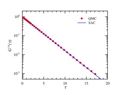
Figure 3: (Color online) The normalized imaginary-time correlation function $G^{xx}(\tau)$ at the wave vector $q=\pi$ for the $S=1$ Heisenberg chain with $D/J=0$, $L=64$ and $\beta=128$, computed in stochastic series expansion QMC calculations. The error bars are much smaller than the symbols. The straight line (blue solid line) corresponds to the contribution from the single-magnon peak obtained from SAC, with the amplitude $a_{0}=0.97375(25)$ and the energy gap $\Delta\approx 0.4104J$.

III NUMERICAL RESULTS

Here, we consider a $S=1$ Heisenberg antiferromagnetic chain of $L=64$ with periodic boundary condition and the inverse temperature $\beta=1/T=2L$ unless specifically mentioned. For positive $D$, the lowest-lying excitations are extracted in the transverse dynamic spin structure factor. In the paper, we study the transverse dynamic spin structure factor $S^{xx}(q,\omega)$ of the topological Haldane phase and its phase transition to the topologically trivial large-$D$ phase.

III.1 Transverse dynamic spin structure

In the Haldane phase Becker et al. (2017); Kennedy and Tasaki (1992); Lu et al. (2016), we assume an isotropic case, i.e. $D/J=0$. In Fig. 2(a), we show the results of the transverse dynamic spin structure factor $S^{xx}(q,\omega)$ obtained from QMC-SAC calculations. The most prominent contribution to excitation spectra is the single-magnon peak, with a lowest energy gap of $\Delta\approx 0.41J$ at the wave vector $q=\pi$. The energy gap $\Delta$ in our methods is given simply by the imaginary-time correlation function

$$G_{q=\pi}^{xx}(\tau)\approx a_{0}e^{-\Delta\tau},$$ (7)

where $a_{0}$ is amplitude of the single-magnon peak. As shown in Fig. 3, the transverse imaginary-time correlation function $G^{xx}(\tau)$ obtained from stochastic series expansion QMC calculations is exponential decay at the wave vector $q=\pi$. It is easy to extract the energy gap $\Delta\approx 0.41J$ from the fitting to Eq. (7). The excitation spectra is a single-magnon peak followed by extremely weak multimagnon continua at higher frequencies, so we provide special treatment to the single-magnon $\delta$ function at the lowest frequency when optimizing the candidate spectral function Shao et al. (2017). In SAC, we also obtain that the amplitude of the single-magnon $\delta$ function is $a_{0}=0.97375(25)$ and its energy gap is $\Delta\approx 0.4104J$ with higher accuracy. The contribution of the single-magnon excitation obtained from SAC nearly coincides with the real transverse imaginary-time correlation function $G^{xx}(\tau)$ as shown in Fig. 3. The single-magnon peak of momenta $q$ is displayed in Fig. 4. The results obtained from QMC-SAC are perfectly consistent with the previous DMRG results White and Affleck (2008). Thus, our numerical methods and results are accurate and reliable enough.

In addition, in Fig. 2(a), the two-magnon and three-magnon continua can also be observed near the wave vectors $q=0$ and $q=\pi$, respectively, although their spectral weights are very small. The inset of Figure 5(b) presents the three-magnon continuum at $q=\pi$ starting at higher frequency $3\Delta$. The spectral weight of the three-magnon continuum at $q=\pi$ is $2.7\%$ compared to the single-magnon peak from SAC. These results are proved to be well matched with previous work White and Affleck (2008). We have reason to believe that the elementary excitations of the Haldane phase are the bosonic magnons Tu et al. (2008).

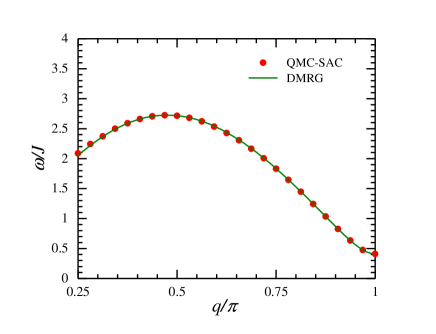
Figure 4: (Color online) The single-magnon dispersion. The red circles show QMC-SAC data for single-magnon peak ($\delta$ function) at the lower frequency bound. The curve (green solid line) is the DMRG results according to Ref. White and Affleck (2008).

The ground state of the topologically trivial large-$D$ phase includes the product state with $S^{z}=0$ at every site if the single-ion anisotropy $D$ is strong enough. Here, we choose an anisotropy $D/J=1.5$ for this phase. Predictably, the lowest-lying excitations can be viewed as single up or down spins that move in a background of ground state with $S^{z}=0$ Lange et al. (2018). The quasiparticle excitations can be termed as excitons and antiexcitons, which reside in the $S^{z}=\pm 1$ branch as shown in Fig. 2(c). Apparently, the large-$D$ phase also has an energy gap. A prominent peak can be observed near the wave vector $q=\pi$ and we consider it as single-exciton excitation. Besides, the extremely weak continua emerge at high frequencies similar to the Haldane phase (see Fig. 5). We suppose that they are multi-excitons and exciton-antiexciton bound states because of the interaction between opposite spins.

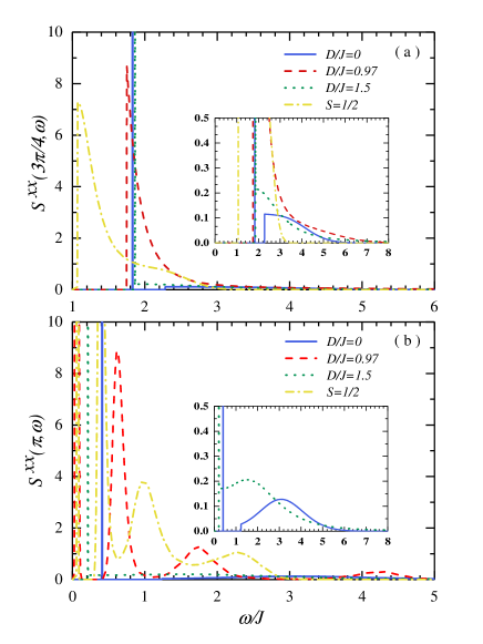
Figure 5: (Color online) The transverse dynamic spin structure factor $S^{xx}(q,\omega)$ of the $S=1$ and $S=1/2$ chains with $L=64$ and $\beta=128$ at two momenta, (a) $q=3\pi/4$ and (b) $q=\pi$. The $S=1$ Heisenberg chain is calculated with three different anisotropies, including $D/J=0$ (blue solid line), $D/J=0.97$ (red dashed line) and $D/J=1.5$ (green dotted line). The blue solid line and green dotted line both have a very sharp peak. The red dashed lines, at the quantum critical point, possess a broad continuum similar to the $S=1/2$ chain (yellow dot-dash line).

Next, we focus on the quantum critical point that belongs to the TLL with a single-ion anisotropy $D/J\approx 0.97$ in Fig. 1. The accuracy of the critical point is high enough for the calculations of the dynamical spin excitations and therefore the single-ion anisotropy $D/J=0.97$ can be treated as the critical value of the quantum phase transition point. A symmetry-protected topological phase cannot be continuously changed into a trivial gapped phase without closing the energy gap, so we are easy to know the critical point is gapless. However, there is no well-defined quasiparticle excitations. Recently, the TLL phase of the $S=1/2$ chain has been realized experimentally, which verified that it possessed a broad continuum and its excitations are fractionalized spinons. From the spin excitation spectra shown in Fig. 2(b), gapless excitations appear at the wave vector $q=\pi$. Moreover, there is a broad continuum near $q=\pi$, which seems like the $S=1/2$ case.

Figure 5 shows the transverse dynamic spin structure factor $S^{xx}(3\pi/4,\omega)$ and $S^{xx}(\pi,\omega)$ of the $S=1/2$ Heisenberg antiferromagnetic chain and the $S=1$ chain in the Haldane phase, the TLL critical state and the large-$D$ phase. We further find that the excitation spectra of the TLL state has a broader continuum than the Haldane phase and the large-D phase, meanwhile with the similar shape to the $S=1/2$ case, which has a high-frequency tail. To conclude, the quasiparticle excitations of the $S=1$ chain are spinon continuum excitations at the quantum critical point.

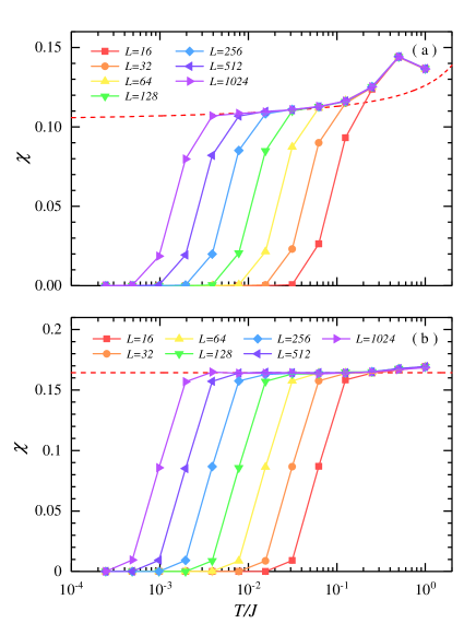
Figure 6: (Color online) (a) The uniform magnetic susceptibility of the $S=1/2$ Heisenberg chain. The red dashed curve is a fitting line based on Eq. (8) with $v=\pi/2$ and $T_{0}=7.7$. (b) The uniform magnetic susceptibility of the $S=1$ Heisenberg chain in the TLL critical state. Both of them are obtained from the QMC calculations. The error bars are much smaller than the symbols.

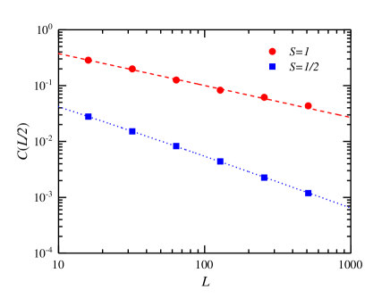
Figure 7: (Color online) The transverse spin-spin correlation function obtained from the QMC calculations for the $S=1$ Heisenberg chain in the TLL critical state and the $S=1/2$ Heisenberg antiferromagnetic chain with $L=16,32,64,128,256,512$ and $\beta=1024$. The error bars are much smaller than the symbols. The red dashed line shows the form $\propto L^{-\alpha}$ with $\alpha=0.57(2)$ for $S=1$. We consider a logarithmic correction $ln^{1/2}(L/L_{0})L^{-\alpha}$ for $S=1/2$ (blue dotted line) with $L_{0}=0.35(6)$ and $\alpha=1$.

III.2 Uniform magnetic susceptibility

We further identify that the low-energy excitations are fractionalized spinons in the TLL critical state of the $S=1$ chain, which can be compared with a $S=1/2$ Heisenberg antiferromagnetic chain. From the low-energy field theory, the uniform magnetic susceptibility of the $S=1/2$ Heisenberg chain has the form Eggert et al. (1994); Frischmuth et al. (1997)

$$\chi(T)=\frac{1}{2\pi v}+\frac{1}{4\pi v\ln(T_{0}/T)},$$ (8)

where $v$ is the spinon velocity. As shown in Fig. 6(a), the dashed curve is the low-$T$ form Eq. (8) of the $S=1/2$ Heisenberg antiferromagnetic chain with $v=\pi/2$ and $T_{0}=7.7$ Eggert et al. (1994). The uniform magnetic susceptibility of the $S=1/2$ chain has been well studied before. We offer the details here in order to compare with the $S=1$ case.

In Fig. 6(b), we presents the uniform magnetic susceptibility of the $S=1$ Heisenberg chain in the TLL critical state with the chain length $L=2^{n}$, where $n=4,5,...,10$. Because of the finite-size effects, the uniform magnetic susceptibility always decays to zero below a temperature $T~{}(\sim 1/L)$. For the $S=1$ chain, the log-linear scale makes the finite-size effects very clear and displays that the uniform magnetic susceptibility satisfies $\chi(T)\approx 0.16439(9)$ in the low temperature as shown in Fig. 6(b). This behavior is different from the $S=1/2$ chain. Thus, in the TLL state, the uniform magnetic susceptibility $\chi(T)$ of the $S=1$ chain will not alter with $T$ in the low temperature in the $L\to\infty$ limit, which is similar to the free fermion gas. The TLL critical state of the $S=1$ chain is paramagnetic and here we can regard the spinon excitations as bosons in this phase.

III.3 Transverse spin-spin correlation function

Additionally, we extract the transverse spin-spin correlation function $C(r)=\langle S^{x}_{i}\cdot S^{x}_{i+r}\rangle$ of the $S=1$ chain in the TLL critical state. We know the spin-spin correlation function $\langle S_{i}\cdot S_{i+r}\rangle$ of a $S=1/2$ Heisenberg antiferromagnetic chain has a power-law distribution as $(-1)^{r}/r$ while $C(r)$ of a isotropic $S=1$ chain decays exponentially with diatance $r$ as $(-1)^{r}r^{-1/2}e^{-r/\xi}$ Haldane (1983b); Takahashi (1988).

In the TLL critical state, the transverse spin-spin correlation function $C(L/2)$ of the $S=1$ chain at the largest distance $r=L/2$ is shown versus the chain length $L$ and compared with a $S=1/2$ Heisenberg antiferromagnetic chain in Fig. 7. For the $S=1$ chain, the transverse spin-spin correlation function has a power-law decay like the $S=1/2$ case, which is different from the Haldane phase. The decay of the $S=1$ chain is $\propto L^{-\alpha}$ with the exponent $\alpha=0.57(2)$ in the TLL critical state. For the $S=1/2$ chain, we consider a multiplicative logarithmic correction $ln^{1/2}(L/L_{0})L^{-\alpha}$ with $\alpha=1$. The exponents of the $S=1$ and $S=1/2$ chains are different, but it is worth mentioning that they both have power-law correlations. Therefore, in the TLL critical state, the low-energy excitations of the $S=1$ Heisenberg chain are fractionalized spinons, just like a $S=1/2$ Heisenberg antiferromagnetic chain. Moreover, the $S=1/2$ chain has an emergent symmetry described by the SU(2) level-1 Wess-Zumino-Witten conformal field theory, which makes the spinon excitations available Rao et al. (2016b); Melko and Kaul (2008). Nevertheless, at the topological quantum critical point of the $S=1$ Heisenberg chain, there is a U(1) spin rotational symmetry. They may belong to different universality classes and it is worthy of further research.

IV DISCUSSION AND CONCLUSION

In this work, we have investigated the transverse dynamic spin structure factor $S^{xx}(q,\omega)$ of the $S=1$ Heisenberg antiferromagnetic chain versus the single-ion anisotropy $D$. We have uncovered the quantum phase diagram, comprising the Néel phase, the Haldane phase, the TLL critical state and the large-$D$ phase, especially their spin dynamics and elementary excitations. At the topological quantum critical point of topological phase transition between the Haldane phase and the large-$D$ phase, a broad continuum has been found near $q=\pi$ and precisely its dynamics are similar to a $S=1/2$ Heisenberg antiferromagnetic chain, which has been verified in various ways. So in the TLL state, the excitations of the $S=1$ Heisenberg antiferromagnetic chain also are fractionalized spinons.

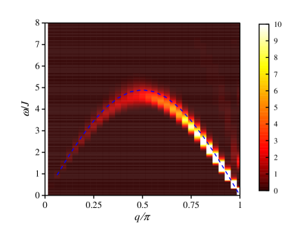
Figure 8: The dynamic spin structure factor $S(q,\omega)$ of the $S=2$ Heisenberg antiferromagnetic chain with $L=64$ and $\beta=16$. The blue dashed line is the magnon dispersion law with the form $\omega(q)=2J\sqrt{S(S+1)}sin(q)$ Meshkov (1993).

Finally, we have extracted the dynamic spin structure factor of the $S=2$ Heisenberg antiferromagnetic chain Schollwock et al. (1996); Schollwoeck and Jolicoeur (1995); Yamamoto (1996); Meshkov (1993) as shown in Fig. 8. In contrast to the topological Haldane phase of the $S=1$ chain, the even-integral spin chain only has a topologically trivial gapped phase with a very small energy gap without a topological quantum phase transition Chen et al. (2013); Gu and Wen (2009). A prominent continuum of the $S=2$ chain can be observed and it seems to coincide with the previous results $\omega(q)=2J\sqrt{S(S+1)}sin(q)$ Meshkov (1993).