PowerNorm: Rethinking Batch Normalization in Transformers

Abstract

The standard normalization method for neural network (NN) models used in Natural Language Processing (NLP) is layer normalization (LN). This is different than batch normalization (BN), which is widely-adopted in Computer Vision. The preferred use of LN in NLP is principally due to the empirical observation that a (naive/vanilla) use of BN leads to significant performance degradation for NLP tasks; however, a thorough understanding of the underlying reasons for this is not always evident. In this paper, we perform a systematic study of NLP transformer models to understand why BN has a poor performance, as compared to LN. We find that the statistics of NLP data across the batch dimension exhibit large fluctuations throughout training. This results in instability, if BN is naively implemented. To address this, we propose Power Normalization (PN), a novel normalization scheme that resolves this issue by (i) relaxing zero-mean normalization in BN, (ii) incorporating a running quadratic mean instead of per batch statistics to stabilize fluctuations, and (iii) using an approximate backpropagation for incorporating the running statistics in the forward pass. We show theoretically, under mild assumptions, that PN leads to a smaller Lipschitz constant for the loss, compared with BN. Furthermore, we prove that the approximate backpropagation scheme leads to bounded gradients. We extensively test PN for transformers on a range of NLP tasks, and we show that it significantly outperforms both LN and BN. In particular, PN outperforms LN by 0.4/0.6 BLEU on IWSLT14/WMT14 and 5.6/3.0 PPL on PTB/WikiText-103. We make our code publicly available at https://github.com/sIncerass/powernorm.

1 Introduction

Normalization has become one of the critical components in Neural Network (NN) architectures for various machine learning tasks, in particular in Computer Vision (CV) and Natural Language Processing (NLP). However, currently there are very different forms of normalization used in CV and NLP. For example, Batch Normalization (BN) (Ioffe & Szegedy, 2015) is widely adopted in CV, but it leads to significant performance degradation when naively used in NLP. Instead, Layer Normalization (LN) (Ba et al., 2016) is the standard normalization scheme used in NLP. All recent NLP architectures, including Transformers (Vaswani et al., 2017), have incorporated LN instead of BN as their default normalization scheme. In spite of this, the reasons why BN fails for NLP have not been clarified, and a better alternative to LN has not been presented.

In this work, we perform a systematic study of the challenges associated with BN for NLP, and based on this we propose Power Normalization (PN), a novel normalization method that significantly outperforms LN. In particular, our contributions are as follows:

• We find that there are clear differences in the batch statistics of NLP data versus CV data. In particular, we observe that batch statistics for NLP data have a very large variance throughout training. This variance exists in the corresponding gradients as well. In contrast, CV data exhibits orders of magnitude smaller variance. See Figure  2 and 3 for a comparison of BN in CV and NLP.

• To reduce the variation of batch statistics, we modify typical BN by relaxing zero-mean normalization, and we replace the variance with the quadratic mean. We denote this scheme as PN-V. We show theoretically that PN-V preserves the first-order smoothness property as in BN; see Lemma 2.

• We show that using running statistics for the quadratic mean results in significantly better performance, up to 1.5/2.0 BLEU on IWSLT14/WMT14 and 7.7/3.4 PPL on PTB/WikiText-103, as compared to BN; see Table 1 and 2. We denote this scheme as PN. Using running statistics requires correcting the typical backpropagation scheme in BN. As an alternative, we propose an approximate backpropagation to capture the running statistics. We show theoretically that this approximate backpropagation leads to bounded gradients, which is a necessary condition for convergence; see Theorem 4.

• We perform extensive tests showing that PN also improves performance on machine translation and language modeling tasks, as compared to LN. In particular, PN outperforms LN by 0.4/0.6 BLEU on IWSLT14/WMT14, and by 5.6/3.0 PPL on PTB/WikiText-103. We emphasize that the improvement of PN over LN is without any change of hyper-parameters.

• We analyze the behaviour of PN and LN by computing the Singular Value Decomposition of the resulting embedding layers, and we show that PN leads to a more well-conditioned embedding layer; see Figure  6. Furthermore, we show that PN is robust to small-batch statistics, and it still achieves higher performance, as opposed to LN; see Figure  5.

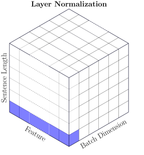
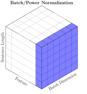
Figure 1: The illustration of layer normalization (left) and batch/power normalization (right). The entries colored in blue show the components used for calculating the statistics.

2 Related Work

Normalization is widely used in modern deep NNs such as ResNet (He et al., 2016), MobileNet-V2 (Sandler et al., 2018), and DenseNet (Huang et al., 2017) in CV, as well as LSTMs (Hochreiter & Schmidhuber, 1997; Ba et al., 2016), transformers (Vaswani et al., 2017), and transformer-based models (Devlin et al., 2019; Liu et al., 2019) in NLP. There are two main categories of normalization: weight normalization (Salimans & Kingma, 2016; Miyato et al., 2018; Qiao et al., 2019) and activation normalization (Ioffe & Szegedy, 2015; Jarrett et al., 2009; Krizhevsky et al., 2012; Ba et al., 2016; Ulyanov et al., 2016; Wu & He, 2018; Li et al., 2019). Here, we solely focus on the latter, and we briefly review related work in CV and NLP.

Normalization in Computer Vision

Batch Normalization (BN) (Ioffe & Szegedy, 2015) has become the de-facto normalization for NNs used in CV. BN normalizes the activations (feature maps) by computing channel-wise mean and variance across the batch dimension, as schematically shown in Figure  1. It has been found that BN leads to robustness with respect to sub-optimal hyperparameters (e.g., learning rate) and initialization, and it generally results in more stable training for CV tasks (Ioffe & Szegedy, 2015). Following the seminal work of (Ioffe & Szegedy, 2015), there have been two principal lines of research: (i) extensions/modifications of BN to improve its performance, and (ii) theoretical/empirical studies to understand why BN helps training.

With regard to (i), it was found that BN does not perform well for problems that need to be trained with small batches, e.g., image segmentation (often due to memory limits) (Zagoruyko & Komodakis, 2016; Lin et al., 2017; Goldberger et al., 2005). The work of (Ioffe, 2017) proposed batch renormalization to remove/reduce the dependence of batch statistics to batch size. It was shown that this approach leads to improved performance for small batch training as well as cases with non-i.i.d. data. Along this direction, the work of (Singh & Shrivastava, 2019) proposed “EvalNorm,” which uses corrected normalization statistics. Furthermore, the recent work of (Yan et al., 2020) proposed “Moving Average Batch Normalization (MABN)” for small batch BN by replacing batch statistics with moving averages.

There has also been work on alternative normalization techniques, and in particular Layer Normalization (LN), proposed by (Ba et al., 2016). LN normalizes across the channel/feature dimension as shown in Figure  1. This could be extended to Group Norm (GN) (Wu & He, 2018), where the normalization is performed across a partition of the features/channels with different pre-defined groups. Instance Normalization (IN) (Ulyanov et al., 2016) is another technique, where per-channel statistics are computed for each sample.

With regard to (ii), there have been several studies to understand why BN helps training in CV. The original motivation was that BN reduces the so-called “Internal Covariance Shift” (ICS) (Ioffe & Szegedy, 2015). However, this explanation was viewed as incorrect/incomplete (Rahimi, 2017). In particular, the recent study of (Santurkar et al., 2018) argued that the underlying reason that BN helps training is that it results in a smoother loss landscape. This was later confirmed for deep NN models by measuring the Hessian spectrum of the network with/without BN (Yao et al., 2019).

Normalization in Natural Language Processing

Despite the great success of BN in CV, the large computation and storage overhead of BN at each time-step in recurrent neural networks (RNNs) made it impossible/expensive to deploy for NLP tasks (Cooijmans et al., 2017). To address this, the work of (Cooijmans et al., 2017; Hou et al., 2019) used shared BN statistics across different time steps of RNNs. However, it was found that the performance of BN is significantly lower than LN for NLP. For this reason, LN became the default normalization technique, even for the recent transformer models introduced by (Vaswani et al., 2017).

Only limited recent attempts were made to compare LN with other alternatives or investigate the reasons behind the success of LN in transformer models. For instance, (Zhang & Sennrich, 2019) proposes RMSNorm, which removes the re-centering invariance in LN and performs re-scaling invariance with the root mean square summed of the inputs. They showed that this approach achieves similar performance to LN, but with smaller (89% to 64%) overhead. Furthermore, (Nguyen & Salazar, 2019) studies different variants of weight normalization for transformers in low-resource machine translation. The recent work of (Xu et al., 2019) studies why LN helps training, and in particular it finds that the derivatives of LN help recenter and rescale backward gradients. From a different angle, (Zhang et al., 2019b, a) try to ascribe the benefits of LN to solving the exploding and vanishing gradient problem at the beginning of training. They also propose two properly designed initialization schemes which also enjoy that property and are able to stabilize training for transformers.

However, most of these approaches achieve similar or marginal improvement over LN. More importantly, there is still not a proper understanding of why BN performs poorly for transformers applied to NLP data. Here, we address this by systematically studying the BN behavior throughout training; and, based on our results, we propose Power Normalization (PN), a new normalization method that significantly outperforms LN for a wide range of tasks in NLP.

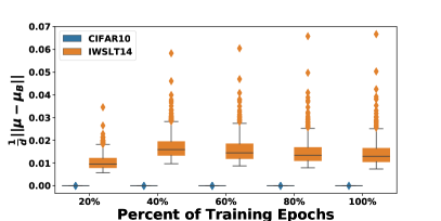
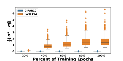
Figure 2: The average Euclidean distance between the batch statistics (${\mu}_{B}$, ${\sigma}_{B}^{2}$) and the running statistics ($\mu$, $\sigma^{2}$) stored in first BN during forward pass for ResNet20 on Cifar-10 and Transformer on IWLST14. We can clearly see that the ResNet20 statistics have orders of magnitude smaller variation than the running statistics throughout training. However, the corresponding statistics in Transformer${}_{\textsc{BN}}$ exhibit very high variance with extreme outliers. This is true both for the mean (shown in the left) as well as variance (shown in right). This is one of the contributing factors to the low performance of BN in transformers.

Algorithm 1 Batch Normalization (Every Iteration)

begin Forward Propagation:

       Input: ${\bm{X}}\in{\bm{R}}^{B\times d}$ Output: ${\bm{Y}}\in{\bm{R}}^{B\times d}$ ${\mu}_{B}=\frac{1}{B}\sum_{i=1}^{B}{\bm{x}}_{i}$

        // Get mini-batch mean ${\sigma}_{B}^{2}=\frac{1}{B}\sum_{i=1}^{B}({\bm{x}}_{i}-{\mu}_{B})^{2}$

        // Get mini-batch variance $\widecheck{\bm{X}}=\frac{{\bm{X}}-{\mu}_{B}}{{\sigma}_{B}}$

        // Normalize ${\bm{Y}}=\gamma\odot\widecheck{\bm{X}}+\beta$

        // Scale and shift $\mu=\alpha\mu+(1-\alpha){\mu}_{B}$

        // Update running mean $\sigma^{2}=\alpha\sigma^{2}+(1-\alpha){\sigma}_{B}^{2}$

        // Update running variance

begin Backward Propagation:

       Input: $\frac{\partial\mathcal{L}}{\partial{\bm{Y}}}\in{\bm{R}}^{B\times d}$ Output: $\frac{\partial\mathcal{L}}{\partial{\bm{X}}}\in{\bm{R}}^{B\times d}$ $\frac{\partial\mathcal{L}}{\partial{\bm{X}}}$ based on Eq. 3

        // Gradient of ${\bm{X}}$

Inference: ${\bm{Y}}=\gamma\odot\frac{{\bm{X}}-\mu}{\sigma}+\beta$

3 Batch Normalization

Notation. We denote the input of a normalization layer as ${\bm{X}}\in{\mathbb{R}}^{B\times d}$, where $d$ is the embedding/feature size and $B$ is the batch size. We denote $\mathcal{L}$ as the final loss of the NN. The i-th row (column) of a matrix, e.g., ${\bm{X}}$, is denoted by ${\bm{X}}_{i,:}$ (${\bm{X}}_{:,i}$). We also write the i-th row of the matrix as its lower-case version, i.e., ${\bm{x}}_{i}={\bm{X}}_{i,:}$. For a vector y, $y_{i}$ denotes the i-th element in y.

Without other specification: (i) for two vector ${\textnormal{x}}\in{\mathbb{R}}^{d}$ and ${\textnormal{y}}\in{\mathbb{R}}^{d}$, we denote xy as the element-wise product, ${\textnormal{x}}+{\textnormal{y}}$ as the element-wise sum, and $\langle{\textnormal{x}},{\textnormal{y}}\rangle$ as the inner product; (ii) for a vector ${\textnormal{y}}\in{\mathbb{R}}^{d}$ and a matrix ${\bm{X}}\in{\mathbb{R}}^{B\times d}$, we denote ${\textnormal{y}}\odot{\bm{X}}$ as $[y_{1}{\bm{X}}_{:,1},...,y_{d}{\bm{A}}_{:,d}]$ and ${\textnormal{y}}+{\bm{X}}$ as $[{\textnormal{y}}+{\bm{X}}_{1,:};...;{\textnormal{y}}+{\bm{X}}_{B,:}]$; and (iii) for a vector ${\textnormal{y}}\in{\mathbb{R}}^{d}$, ${\textnormal{y}}>C$ means that each entry of y is larger than the constant $C$, i.e., $y_{i}>C$ for all $i$.

3.1 Formulation of Batch Normalization

We briefly review the formulation of BN (Ioffe & Szegedy, 2015). Let us denote the mean (variance) of ${\bm{X}}$ along the batch dimension as ${\mu}_{B}\in{\mathbb{R}}^{d}$ (${\sigma}_{B}^{2}\in{\mathbb{R}}^{d}$). The batch dimension is illustrated in Figure  1. The BN layer first enforces zero mean and unit variance, and it then performs an affine transformation by scaling the result by $\gamma,\beta\in{\mathbb{R}}^{d}$, as shown in Algorithm 1.

The Forward Pass (FP) of BN is performed as follows. Let us denote the intermediate result of BN with zero mean and unit variance as $\widecheck{\bm{X}}$, i.e.,

$$\widecheck{\bm{X}}=\frac{{\bm{X}}-{\mu}_{B}}{{\sigma}_{B}}.$$ (1)

The final output of BN, ${\bm{Y}}$, is then an affine transformation applied to $\widecheck{\bm{X}}$:

$${\bm{Y}}=\gamma\odot\widecheck{\bm{X}}+\beta.$$ (2)

The corresponding Backward Pass (BP) can then be derived as follows. Assume that the derivative of $\mathcal{L}$ with respect to ${\bm{Y}}$ is given, i.e., $\frac{\partial\mathcal{L}}{\partial{\bm{Y}}}$ is known. Then, the derivative with respect to input can be computed as:

$$\frac{\partial\mathcal{L}}{\partial{\bm{x}}_{i}}=\frac{\gamma}{{\sigma}_{B}}\frac{\partial\mathcal{L}}{\partial{\bm{y}}_{i}}-\frac{\gamma}{{\sigma}_{B}B}\sum_{j\in B}(\underbrace{\frac{\partial\mathcal{L}}{\partial{\bm{y}}_{j}}}_{\text{from ${\mu}_{B}$: $g_{\mu}$}}+\underbrace{\frac{\partial\mathcal{L}}{\partial{\bm{y}}_{j}}\check{\bf x}_{j}\check{\bf x}_{i}}_{\text{from ${\sigma}_{B}^{2}$: $g_{\sigma^{2}}$}}).$$ (3)

See Lemma 6 in Appendix C for details. We denote the terms contributed by ${\mu}_{B}$ and ${\sigma}_{B}^{2}$ as $g_{\mu}$ and $g_{\sigma^{2}}$, respectively.

In summary, there are four batch statistics in BN, two in FP and two in BP. The stability of training is highly dependent on these four parameters. In fact, naively implementing the BN as above for transformers leads to poor performance. For example, using transformer with BN (denoted as Transformer${}_{\textsc{BN}}$) results in 1.1 and 1.4 lower BLEU score, as compared to the transformer with LN (Transformer${}_{\textsc{LN}}$), on IWSLT14 and WMT14, respectively; see Table 1.

This is significant performance degradation, and it stems from instabilities associated with the above four batch statistics. To analyze this, we studied the batch statistics using the standard setting of ResNet20 on Cifar-10 and Transformer${}_{\textsc{BN}}$ on IWSLT14 (using a standard batch size of 128 and tokens of 4K, respectively). In the first experiment, we probed the fluctuations between batch statistics, ${\mu}_{B}$/${\sigma}_{B}$, and the corresponding BN running statistics, $\mu$/$\sigma$, throughout training. This is shown for the first BN layer of ResNet20 on Cifar-10 and Transformer${}_{\textsc{BN}}$ on IWSLT14 in Figure  2. Here, the y-axis shows the average Euclidean distance between batch statistics (${\mu}_{B}$, ${\sigma}_{B}$) and the running statistics ($\mu$, $\sigma$), and the x-axis is different epochs of training, where we define the average Euclidean distance as $\text{dist}({\mu}_{B},\mu)=\frac{1}{d}\|{\mu}_{B}-\mu\|$.

The first observation is that Transformer${}_{\textsc{BN}}$ shows significantly larger distances between the batch statistics and the running statistics than ResNet20 on Cifar-10, which exhibits close to zero fluctuations. Importantly, this distance between ${\sigma}_{B}$ and $\sigma$ significantly increases throughout training, but with extreme outliers. During inference, we have to use the running statistics. However, such large fluctuations would lead to a large inconsistency between statistics of the testing data and the BN’s running statistics.

The second observation comes from probing the norm of $g_{\mu}$ and $g_{\sigma^{2}}$ defined in Eq. 3, which contribute to the gradient backpropagation of input. These results are shown in Figure  3, where we report the norm of these two parameters for ResNet20 and Transformer${}_{\textsc{BN}}$. For Transformer${}_{\textsc{BN}}$, we can see very large outliers that actually persist throughout training. This is in contrast to ResNet20, for which the outliers vanish as training proceeds.

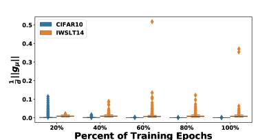
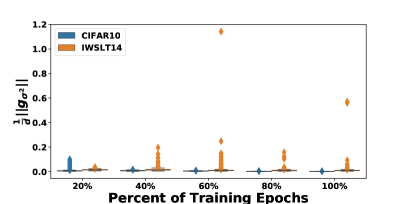
Figure 3: The average gradient norm of the input of the first BN layer contributed by ${\mu}_{B}$ and ${\sigma}_{B}$ for ResNet20 on Cifar10 and Transformer${}_{\textsc{BN}}$ on IWSLT14 during the BP (note that $d=16$ for Cifar-10 and $d=512$ for IWSLT experiment). It can be clearly seen that the norm of $g_{\mu}$ and $g_{\sigma^{2}}$ for ResNet20 has orders of magnitude smaller variation throughout training, as compared to that for Transformer${}_{\textsc{BN}}$. Also, the outliers for ResNet20 vanish at the end of training, which is in contrast to Transformer${}_{\textsc{BN}}$, for which the outliers persist. This is true both for $g_{\mu}$ (shown in left) as well as $g_{\sigma^{2}}$ (shown in right).

4 Power Normalization

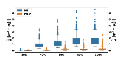
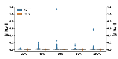
Figure 4: Results for Transformer on IWSLT14. (Left) The average Euclidean distance between batch statistics (${\sigma}_{B}$, ${{\psi_{B}}}$) and the running statistics ($\sigma$, $\psi$) stored in first BN/PN-V during forward propagation (FP). (Right) The average norm of gradient of the input of the first BN/PN-V contributed by ${\sigma}_{B}$/${{\psi_{B}}}$. During FP, ${{\psi_{B}}}$ has much smaller variations of running statistics, as compared to ${\sigma}_{B}$, as shown in left, It can also be clearly seen that during BP, the norm of $g_{\psi^{2}}$ exhibits many fewer outliers, as compared to $g_{\sigma^{2}}$, throughout the training.

Based on our empirical observations, we propose Power Normalization (PN), which effectively resolves the performance degradation of BN. This is achieved by incorporating the following two changes to BN. First, instead of enforcing unit variance, we enforce unit quadratic mean for the activations. The reason for this is that we find that enforcing zero-mean and unit variance in BN is detrimental due to the large variations in the mean, as discussed in the previous section. However, we observe that unlike mean/variance, the unit quadratic mean is significantly more stable for transformers. Second, we incorporate running statistics for the quadratic mean of the signal, and we incorporate an approximate backpropagation method to compute the corresponding gradient. We find that the combination of these two changes leads to a significantly more effective normalization, with results that exceed LN, even when the same training hyper-parameters are used. Below we discuss each of these two components.

4.1 Relaxing Zero-Mean and Enforcing Quadratic Mean

Here, we describe the first modification in PN. As shown in Figure  2 and 3, ${\mu}_{B}$ and $g_{\mu}$ exhibit significant number of large outliers, which leads to inconsistencies between training and inference statistics. We first address this by relaxing the zero-mean normalization, and we use the quadratic mean of the signal, instead of its variance. The quadratic mean exhibits orders of magnitude smaller fluctuations, as shown in Figure  4. We refer to this normalization (i.e., no zero mean and unit quadratic mean enforcement) as PN-V, defined as follows.

Definition 1 (PN-V).

Let us denote the quadratic mean of the batch as ${{\psi_{B}}}^{2}=\frac{1}{B}\sum_{i=1}^{B}{\bm{x}}_{i}^{2}$. Furthermore, denote $\widehat{\bm{X}}$ as the signal scaled by ${{\psi_{B}}}$, i.e.,

$$\widehat{\bm{X}}=\frac{{\bm{X}}}{{{\psi_{B}}}}.$$ (4)

Then, the output of PN-V is defined as

$${\bm{Y}}=\gamma\odot\widehat{\bm{X}}+\beta,$$ (5)

where $\gamma\in{\mathbb{R}}^{d}$ and $\beta\in{\mathbb{R}}^{d}$ are two parameters (vectors) in PN-V (which is the same as in the affine transformation used in BN).

Note that here we use the same notation ${\bm{Y}}$ as the output in Eq. 2 without confusion.

The corresponding BP of PN-V is as follows:

$$\frac{\partial\mathcal{L}}{\partial{\bm{x}}_{i}}=\frac{\gamma}{{{\psi_{B}}}}\frac{\partial\mathcal{L}}{\partial{\bm{y}}_{i}}-\frac{\gamma}{B{{\psi_{B}}}}\sum_{j\in B}\underbrace{\frac{\partial\mathcal{L}}{\partial{\bm{y}}_{j}}\hat{\bf x}_{j}\hat{\bf x}_{i}}_{\text{from ${{\psi_{B}}}^{2}$: $g_{\psi^{2}}$}}.$$ (6)

See Lemma 8 in Appendix C for the full details. Here, $g_{\psi^{2}}$ is the gradient attributed by ${{\psi_{B}}}^{2}$. Note that, compared to BN, there exist only two batch statistics in FP and BP: ${{\psi_{B}}}^{2}$ and $g_{\psi^{2}}$. This modification removes the two unstable factors corresponding to ${\mu}_{B}$ and ${\sigma}_{B}$ in BN ($g_{\mu}$, and $g_{\sigma^{2}}$ in Eq. 3). This modification also results in significant performance improvement, as reported in Table 1 for IWSLT14 and WMT14. By directly replacing BN with PN-V (denoted as Transformer${}_{\textsc{PN-V}}$), the BLEU score increases from 34.4 to 35.4 on IWSLT14, and 28.1 to 28.5 on WMT14. These improvements are significant for these two tasks. For example, (Zhang et al., 2019b, a) only improves the BLEU score by 0.1 on IWSLT14.

As mentioned before, ${{\psi_{B}}}$ exhibits orders of magnitude smaller variations, as compared to ${\sigma}_{B}$. This is shown in Figure  4, where we report the distance between the running statistics for $\sigma$, $\text{dist}({\sigma}_{B}^{2},\sigma^{2})$, and $\psi$, $\text{dist}({{\psi_{B}}}^{2},\psi^{2})$. Similarly during BP, we compute the norm of $g_{\sigma^{2}}$ and $g_{\psi^{2}}$, and we report it in Figure  4 throughout training. It can be clearly seen that during BP, the norm of $g_{\psi^{2}}$ exhibits many fewer outliers as compared to $g_{\sigma^{2}}$.

In (Santurkar et al., 2018), the authors provided theoretical results suggesting that employing BN in DNNs can lead to a smaller Lipschitz constant of the loss.

It can be shown that PN-V also exhibits similar behaviour, under mild assumptions. In more detail, let us denote the loss of the NN without normalization as $\widehat{\mathcal{L}}$. With mild assumptions, (Santurkar et al., 2018) shows that the norm of $\frac{\partial\mathcal{L}}{\partial{\bm{X}}}$ (with BN) is smaller than the norm of $\frac{\partial\widehat{\mathcal{L}}}{\partial{\bm{X}}}$. Here, we show that, under the same assumptions, PN-V can achieve the same results that BN does. See Appendix C for details, including the statement of Assumption 9.

Lemma 2 (The effect of PN-V on the Lipschitz constant of the loss).

Under Assumption 9, we have

$$\|\frac{\partial\mathcal{L}}{\partial{\bm{X}}_{:,i}}\|^{2}=\frac{\gamma^{2}_{i}}{({{\psi_{B}}})_{i}^{2}}\left(\|\frac{\partial\widehat{\mathcal{L}}}{\partial{\bm{X}}_{:,i}}\|^{2}-\langle\frac{\partial\widehat{\mathcal{L}}}{\partial{\bm{X}}_{:,i}},\frac{\widehat{\bm{X}}_{:,i}}{\sqrt{B}}\rangle^{2}\right).$$ (7)

See the proof in Appendix C. Note that $\langle\frac{\partial\widehat{\mathcal{L}}}{\partial{\bm{X}}_{:,i}},\frac{\widehat{\bm{X}}_{:,i}}{\sqrt{B}}\rangle^{2}$ is non-negative, and hence the Lipschitz constant of $\mathcal{L}$ is smaller than that of $\widehat{\mathcal{L}}$ if $\gamma_{i}\leq({{\psi_{B}}})_{i}$. This is what we observe in practice, as shown in Appendix B.

4.2 Running Statistics in Training

Algorithm 2 Power Normalization (Every Iteration)

begin Forward Propagation:

       Input: ${\bm{X}}\in{\bm{R}}^{B\times d}$ Output: ${\bm{Y}}\in{\bm{R}}^{B\times d}$ ${{\psi_{B}}}^{2}=\frac{1}{B}\sum_{i=1}^{B}{\bm{x}}_{i}^{2}$

        // Get mini-batch statistics $\widehat{\bm{X}}=\frac{{\bm{X}}}{\psi}$

        // Normalize ${\bm{Y}}=\gamma\odot\widehat{\bm{X}}+\beta$

        // Scale and shift $\psi^{2}=\alpha\psi^{2}+(1-\alpha){{\psi_{B}}}^{2}$

        // Update running statistics

begin Backward Propagation:

       Input: $\frac{\partial\mathcal{L}}{\partial{\bm{Y}}}\in{\bm{R}}^{B\times d}$ Output: $\frac{\partial\mathcal{L}}{\partial{\bm{X}}}\in{\bm{R}}^{B\times d}$ $\frac{\partial\mathcal{L}}{\partial\widehat{\bm{X}}}=\gamma\odot\frac{\partial\mathcal{L}}{\partial{\bm{Y}}}$

        // Intermediate Gradient $\widetilde{\bm{X}}^{\prime}=\frac{\partial\mathcal{L}}{\partial\widehat{\bm{X}}}-\nu\widehat{\bm{X}}$

        // Intermediate Estimated Gradient $\frac{\partial\mathcal{L}}{\partial{\bm{X}}}=\frac{\widetilde{\bm{X}}^{\prime}}{\psi}$

        // Gradient of ${\bm{X}}$ $\nu=\nu(1-(1-\alpha)\Gamma)+(1-\alpha)\Lambda$

        // See Definition 3 for $\Gamma$ and $\Lambda$

Inference: ${\bm{Y}}=\gamma\odot\frac{{\bm{X}}}{\psi}+\beta$

Here, we discuss the second modification in PN. First note that even though Transformer${}_{\textsc{PN-V}}$ outperforms Transformer${}_{\textsc{BN}}$, it still can not match the performance of LN. This could be related to the larger number of outliers present in ${{\psi_{B}}}$, as shown in Figure  4. A straightforward solution to address this is to use running statistics for the quadratic mean (denoted as $\psi^{2}$), instead of using per batch statistics, since the latter changes in each iteration. However, using running statistics requires modification of the backpropagation, which we described below.

Definition 3 (PN).

Denote the inputs/statistics at the t-th iteration by $\cdot^{(t)}$, e.g., ${\bm{X}}^{(t)}$ is the input data at t-th iteration. In the forward propagation, the following equations are used for the calculation:

$$\widehat{\bm{X}}^{(t)} =\frac{{\bm{X}}^{(t)}}{\psi^{(t-1)}},$$ (8)

$${\bm{Y}}^{(t)} =\gamma\odot\widehat{\bm{X}}^{(t)}+\beta,$$ (9)

$$(\psi^{(t)})^{2} =(\psi^{(t-1)})^{2}+(1-\alpha)({{\psi_{B}}}^{2}-(\psi^{(t-1)})^{2}).$$ (10)

Here, $0<\alpha<1$ is the moving average coefficient in the forward propagation, and ${{\psi_{B}}}$ is the statistic for the current batch. Since the forward pass evolves running statistics, the backward propagation cannot be accurately computed—namely, the accurate gradient calculation needs to track back to the first iteration. Here, we propose to use the following approximated gradient in backward propagation:

$$(\widetilde{\bm{X}}^{(t)})^{\prime} =\frac{\partial\mathcal{L}}{\partial\widehat{\bm{X}}^{(t)}}-\nu^{(t-1)}\odot\widehat{\bm{X}}^{(t)},$$ (11)

$$\frac{\partial\mathcal{L}}{\partial{\bm{X}}^{(t)})} =\frac{(\widetilde{\bm{X}}^{(t)})^{\prime}}{\psi^{(t-1)}},$$ (12)

$$\nu^{(t)} =\nu^{(t-1)}(1-(1-\alpha)\Gamma^{(t)})+(1-\alpha)\Lambda^{(t)},$$ (13)

where $\Gamma^{(t)}=\frac{1}{B}\sum_{i=1}^{B}\hat{\bf x}_{i}^{(t)}\hat{\bf x}_{i}^{(t)}$ and $\Lambda^{(t)}=\frac{1}{B}\sum_{i=1}^{B}\frac{\partial\mathcal{L}}{\partial\hat{\bf x}_{i}^{(t)}}\hat{\bf x}_{i}^{(t)}$.

This backpropagation essentially uses running statistics by computing the gradient of the loss w.r.t. the quadratic mean of the current batch, rather than using the computationally infeasible method of computing directly the gradient w.r.t. running statistics of the quadratic mean. Importantly, this formulation leads to bounded gradients which is necessary for convergence, as shown below.

Theorem 4 (Gradient of $\mathcal{L}$ w.r.t. ${\bm{X}}$ is bounded in PN).

For any datum point of $\widetilde{\bm{X}}$ (i.e. $\widetilde{\bm{X}}_{i,:}$), the gradients computed from Eq. 11 are bounded by a constant.

Furthermore, the gradient of ${\bm{X}}_{i,:}$ is also bounded, as given Eq. 12.

See the proof in Appendix C. The pseudo-code for PN algorithm is presented in Algorithm 2.

5 Results

5.1 Experiment Setup

We compare our PN method with LN and BN for a variety of sequence modeling tasks: Neural Machine Translation (MT); and Language Modeling (LM). We implement our code for MT using fairseq-py (Ott et al., 2019), and (Ma et al., 2019) for LM tasks. For a fair comparison, we directly replace the LN in transformers (Transformer${}_{\textsc{LN}}$) with BN (Transformer${}_{\textsc{BN}}$) or PN (Transformer${}_{\textsc{PN}}$) without varying the position of each normalization layer or changing the training hyperparameters.

For all the experiments, we use the pre-normalization setting in (Wang et al., 2019), where the normalization layer is located right before the multi-head attention module and point-wise feed-forward network module. Following (Wang et al., 2019), we generally increase the learning rate by a factor of 2.0, relative to the common post-normalization transformer (Vaswani et al., 2017). Below we discuss tasks specific settings.

Neural Machine Translation

We evaluate our methods on two widely used public datasets: IWSLT14 German-to-English (De-En) and WMT14 English-to-German (En-De) dataset. We follow the settings reported in (Ott et al., 2018). We use transformer big architecture for WMT14 (4.5M sentence pairs) and small architecture for IWSLT14 (0.16M sentence pairs). For inference, we average the last 10 checkpoints, and we set the length penalty to 0.6/1.0, and the beam size to 4/5 for WMT/IWSLT, following (Ott et al., 2019). All the other hyperparamters (learning rate, dropout, weight decay, warmup steps, etc.) are set identically to the ones reported in the literature for LN (i.e., we use the same hyperparameters for BN/PN).

Language Modeling

We experiment on both PTB (Mikolov et al., 2011) and Wikitext-103 (Merity et al., 2017), which contain 0.93M and 100M tokens, respectively. We use three layers tensorized transformer core-1 for PTB and six layers tensorized transformer core-1 for Wikitext-103, following (Ma et al., 2019). Furthermore, we apply the multi-linear attention mechanism with masking, and we report the final testing set perplexity (PPL).

Model IWSLT14 WMT14 small big Transformer (Vaswani et al., 2017) 34.4 28.4 DS-Init (Zhang et al., 2019a) 34.4 29.1 Fixup-Init (Zhang et al., 2019b) 34.5 29.3 Scaling NMT (Ott et al., 2018) / 29.3 Dynamic Conv (Wu et al., 2019) 35.2 29.7 Transformer + LayerDrop (Fan et al., 2020) / 29.6 Pre-Norm Transformer${}_{\textsc{LN}}$ 35.5 29.5 Pre-Norm Transformer${}_{\textsc{BN}}$ 34.4 28.1 Pre-Norm Transformer${}_{\textsc{PN-V}}$ 35.5 28.5 Pre-Norm Transformer${}_{\textsc{PN}}$ 35.9 30.1

Table 1: MT performance (BLEU) on IWSLT14 De-En and WMT14 En-De testsets. Using PN-V instead of BN significantly improves the performance, but LN still outperforms. However, PN achieves much higher BLEU scores, as compared to LN.

5.2 Experiment Results

Neural Machine Translation

We use BLEU (Papineni et al., 2002) as the evaluation metric for MT. Following standard practice, we measure tokenized case-sensitive BLEU and case-insensitive BLEU for WMT14 En-De and IWSLT14 De-En, respectively. For a fair comparison, we do not include other external datasets. All the transformers in Table 1 are using six encoder layers and six decoder layers.

The results are reported in Table 1. In the first section of rows, we report state-of-the-art results for these two tasks with comparable model sizes. In the second section of rows, we report the results with different types of normalization. Notice the significant drop in BLEU score when BN is used (34.4/28.1), as opposed to LN (35.5/29.5). Using PN-V instead of BN helps reduce this gap, but LN still outperforms. However, the results corresponding to PN exceeds LN results by more than 0.4/0.6 points, This is significant for these tasks. Comparing with other concurrent works like DS-Init and Fixup-Init (Zhang et al., 2019a, b), the improvements in Transformer${}_{\textsc{PN}}$ are still significant.

Language Modeling

Model	PTB	WikiText-103
	Test PPL	Test PPL
Tied-LSTM (Inan et al., 2017)	48.7	48.7
AWD-LSTM-MoS (Yang et al., 2018)	56.0	29.2
Adaptive Input (Baevski & Auli, 2019)	57.0	20.5
Transformer-XL${}_{\texttt{base}}$ (Dai et al., 2019)	54.5	24.0
Transformer-XL${}_{\texttt{large}}$ (Dai et al., 2019)	–	18.3
Tensor-Transformer${}_{\text{1core}}$ (Ma et al., 2019)	57.9	20.9
Tensor-Transformer${}_{\text{2core}}$ (Ma et al., 2019)	49.8	18.9
Tensor-Transformer${}_{\text{1core}}$ + LN	53.2*	20.9*
Tensor-Transformer${}_{\text{1core}}$ + BN	60.7	27.2
Tensor-Transformer${}_{\text{1core}}$ + PN-V	55.3	21.3
Tensor-Transformer${}_{\text{1core}}$ + PN	47.6	17.9

Table 2: Results with state-of-the-art methods on PTB and WikiText-103. ’-’ indicates no reported results in that setting, ’$*$’ indicates the results are from our own implementation. PN achieves 5.6/3 points lower testing PPL on PTB and WikiTest-103, respectively, compared to LN.

We report the LM results in Table 2, using the tensorized transformer proposed in (Ma et al., 2019). Here we observe a similar trend. Using BN results in a significant degradation, increasing testing PPL by more than 7.5/6.3 for PTB/WikiText-103 datasets (achieving 60.7/27.2 as opposed to 53.2/20.9). However, when we incorporate the PN normalization, we achieve state-of-the-art results for these two tasks (for these model sizes and without any pre-training on other datasets). In particular, PN results in 5.6/3 points lower testing PPL, as compared to LN. Importantly, note that using PN we achieve better results than (Ma et al., 2019), with the same number of parameters.

5.3 Analysis

The Effect of Batch Size for Different Normalization

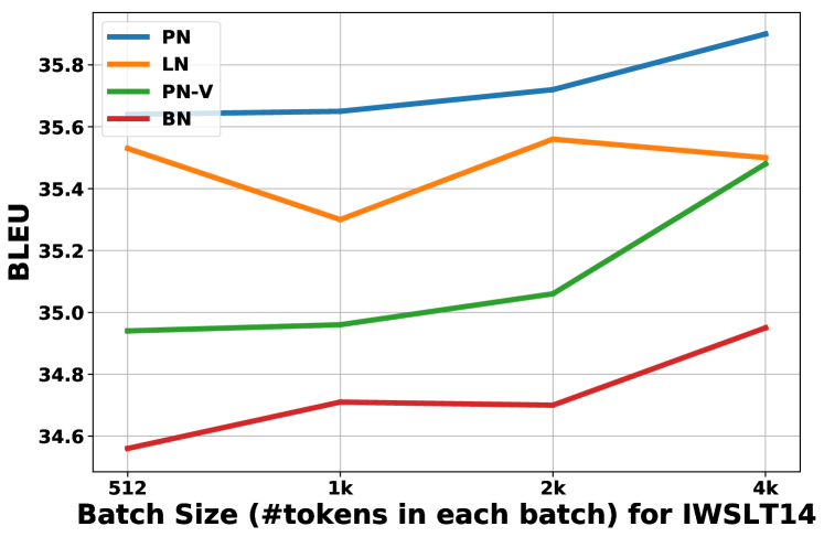
Figure 5: Ablation study of the performance of PN, PN-V, LN and BN on IWSLT14 trained using different batch sizes. Note that the performance of PN consistently outperforms LN. In the meanwhile, PN-V can only match the result of LN when mini-batch gets to 4K. Among all the settings, BN behaves poorly and abnormally across different mini-batches.

To understand better the effects of our proposed methods PN and PN-V, we change the batch size used to collect statistics in BN, LN, and PN. To this end, we keep the total batch size constant at 4K tokens, and we vary the mini-batch size used to collect statistics from 512 to 4K. Importantly, note that we keep the total batch size constant at 4K, and we use gradient accumulation for smaller mini-batches. For example, for the case with mini-batch of 512, we use eight gradient accumulations. The results are reported in Figure  5. We can observe that BN behaves poorly and abnormally across different mini-batches. Noticeably, after relaxing the zero-mean normalization in BN and replacing the variance estimation with quadratic mean, PN-V matches the performance of LN for 4K mini-batch and consistently outperforms BN. However, it underperforms LN. In contrast, we can see that PN consistently achieves higher results under different mini-batch settings.

Representation Power of learned Embedding

To investigate further the performance gain of PN, we compute the Singular Value Decomposition of the embedding layers, as proposed by (Gao et al., 2019), which argued that the singular value distribution could be used as a proxy for measuring representational power of the embedding layer. It has been argued that having fast decaying singular values leads to limiting the representational power of the embeddings to a small sub-space. If this is the case, then it may be preferable to have a more uniform singular value distribution (Wang et al., 2020). We compute the singular values for word embedding matrix of LN and PN, and we report the results in Figure  6. It can be clearly observed that the singular values corresponding to PN decay more slowly than those of LN. Intuitively, one explanation for this might be that PN helps by normalizing all the tokens across the batch dimension, which can result in a more equally distributed embeddings. This may illustrate one of the reasons why PN outperforms LN.

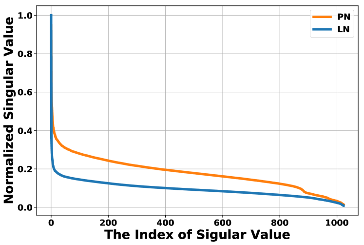
Figure 6: Singular values of embedding matrix trained with LN/PN on WMT14. We normalize the singular values of each matrix so that they are comparable with the largest one as 1. Note that the singular values corresponding to PN decay more slowly than those of LN.

6 Conclusion

In this work, we systematically analyze the ineffectiveness of vanilla batch normalization (BN) in transformers. Comparing NLP and CV, we show evidence that the batch statistics in transformers on NLP tasks have larger variations. This further leads to the poor performance of BN in transformers. By decoupling the variations into FP and BP computation, we propose PN-V and PN to alleviate the variance issue of BN in NLP. We also show the advantages of PN-V and PN, both theoretically and empirically. Theoretically, PN-V preserves the first-order smoothness property as in BN. The approximate backpropagation of PN leads to bounded gradients. Empirically, we show that PN outperforms LN in neural machine translation (0.4/0.6 BLEU on IWSLT14/WMT14) and language modeling (5.6/3.0 PPL on PTB/WikiText-103) by a large margin. We also conduct further analysis of the effect of PN-V/PN/BN/LN under different batch size settings to show the significance of statistical estimations, and we investigate the representation power of learned embeddings matrix by LN/PN to illustrate the effectiveness of PN.

Appendix A Training Details

A.1 Machine Translation.

Dataset

The training/validation/test sets for the IWSLT14 dataset contain about 153K/7K/7K sentence pairs, respectively. We use a vocabulary of 10K tokens based on a joint source and target byte pair encoding (BPE) (Sennrich et al., 2016). For the WMT14 dataset, we follow the setup of (Vaswani et al., 2017), which contains 4.5M training parallel sentence pairs. Newstest2014 is used as the test set, and Newstest2013 is used as the validation set. The 37K vocabulary for WMT14 is based on a joint source and target BPE factorization.

Hyperparameter

Given the unstable gradient issues of decoders in NMT (Zhang et al., 2019a), we only change all the normalization layers in the 6 encoder layers from LN to BN/PN, and we keep all the 6 decoder layers to use LN. For Transformer${}_{\textsc{PN-V}}$ big and Transformer${}_{\textsc{BN}}$ big (not Transformer${}_{\textsc{PN}}$ big), we use the synchronized version, where each FP and BP will synchronize the mean/variance/quadratic mean of different batches at different nodes. For PN, we set the $\alpha$ in the forward and backward steps differently, and we tune the best setting over 0.9/0.95/0.99 on the validation set. To control the scale of the activation, we also involve a layer-scale layer (Zhang & Sennrich, 2019) in each model setting before the normalization layer. The warmup scheme for accumulating $\psi$ is also employed, as suggested in (Yan et al., 2020) . Specifically, we do not tune the warmup steps, but we set it identical to the warmup steps for the learning rate schedule in the optimizer (Vaswani et al., 2017). We set dropout as 0.3/0.0 for Transformer big/small model, respectively. We use the Adam optimizer and follow the optimizer setting and learning rate schedule in (Wang et al., 2019). We set the maximum number of updates following (Ott et al., 2018) to be 300k for WMT and 100k for IWSLT. We used early stopping to stop the experiments by showing no improvement over the last 10/5 epochs. For the big model, we enlarge the batch size and learning rate, as suggested in (Ott et al., 2019), to accelerate training. We employ label smoothing of value $\epsilon_{\text{ls}}=0.1$ in all experiments. We implement our code for MT using fairseq-py (Ott et al., 2019).

Evaluation

We use BLEU (Papineni et al., 2002) as the evaluation metric for MT. Following standard practice, we measure tokenized case-sensitive BLEU and case-insensitive BLEU for WMT14 En-De and IWSLT14 De-En, respectively. For a fair comparison, we do not include other external datasets. For inference, we average the last 10 checkpoints, and we set the length penalty to 0.6/1.0 and beam size to 4/5 for WMT/IWSLT, following (Ott et al., 2019).

A.2 Language Modeling.

Dataset

PTB (Mikolov et al., 2011) has 0.93M training tokens, 0.073M validation words, and 0.082M test word. Wikitext-103 (Merity et al., 2017) contains 0.27M unique tokens, and 100M training tokens from 28K articles, with an average length of 3.6K tokens per article. We use the same evaluation scheme that was provided in (Dai et al., 2019).

Hyperparameter

We use three layers tensorized transformer core-1 for PTB and six layers tensorized transformer core-1 for Wikitext-103, following (Ma et al., 2019). This means there exists only one linear projection in multi-linear attention. We replace every LN layer with a PN layer. For PN, we set the $\alpha$ in forward and backward differently, and we tune the best setting over 0.9/0.95/0.99 on the validation set. The warmup scheme and layer-scale are also the same as the hyperparameter setting introduced for machine translation. We set the dropout as 0.3 in all the datasets. The model is trained using 30 epochs for both PTB and WikiText-103. We use the Adam optimizer, and we follow the learning rate setting in (Ma et al., 2019). We set the warmup steps to be 4000 and label smoothing to be $\epsilon_{\text{ls}}=0.1$ in all experiments.

Appendix B Extra Results

B.1 Empirical Results for Lemma 2.

Under Assumption 9, mentioned in Section 4.1 and discussed in Appendix C.1, we show

$$\|\frac{\partial\mathcal{L}}{\partial{\bm{X}}_{:,i}}\|^{2}=\frac{\gamma^{2}_{i}}{({{\psi_{B}}})_{i}^{2}}\big{(}\|\frac{\partial\widehat{\mathcal{L}}}{\partial{\bm{X}}_{:,i}}\|^{2}-\langle\frac{\partial\widehat{\mathcal{L}}}{\partial{\bm{X}}_{:,i}},\frac{\widehat{\bm{X}}_{:,i}}{\sqrt{B}}\rangle^{2}\big{)}.$$

Given that $\langle\frac{\partial\widehat{\mathcal{L}}}{\partial{\bm{X}}_{:,i}},\frac{\widehat{\bm{X}}_{:,i}}{\sqrt{B}}\rangle^{2}$ is non-negative, the Lipschitz constant of $\mathcal{L}$ is smaller than that of $\widehat{\mathcal{L}}$ if $\gamma_{i}\leq({{\psi_{B}}})_{i}$. Here, we report the empirical results to show that $\gamma_{i}\leq({{\psi_{B}}})_{i}$ holds for each $i\in\{1,2,...,d\}$ on IWSLT14; see Figure  7. Observe that the Lipschitz constant of $\mathcal{L}$ is smaller than that of $\widehat{\mathcal{L}}$ empirically in our setting.

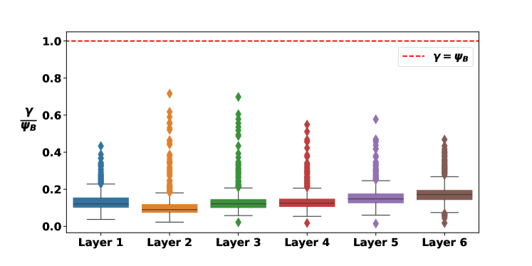
Figure 7: The empirical results of the distribution of $\frac{\gamma}{({{\psi_{B}}})}\in{\mathbb{R}}^{d}$ in different layers of Transformer${}_{\textsc{PN-V}}$ on IWSLT14. Given that $\gamma_{i}\leq({{\psi_{B}}})_{i}$ holds for each $i\in\{1,2,...,d\}$, Lemma 2 holds as well.

B.2 Validation Results on Language Modeling.

Model	PTB		WikiText-103
	Val PPL	Test PPL	Val PPL	Test PPL
Tied-LSTM (Inan et al., 2017)	75.7	48.7	–	48.7
AWD-LSTM-MoS (Yang et al., 2018)	58.1	56.0	29.0	29.2
Adaptive Input (Baevski & Auli, 2019)	59.1	57.0	19.8	20.5
Transformer-XL${}_{\texttt{base}}$ (Dai et al., 2019)	56.7	54.5	23.1	24.0
Transformer-XL${}_{\texttt{large}}$ (Dai et al., 2019)	–	–	–	18.3
Tensor-Transformer${}_{\text{1core}}$ (Ma et al., 2019)	55.4	57.9	23.6	20.9
Tensor-Transformer${}_{\text{2core}}$ (Ma et al., 2019)	54.3	49.8	19.7	18.9
Tensor-Transformer${}_{\text{1core}}$ + LN	58.0*	53.2*	22.7*	20.9*
Tensor-Transformer${}_{\text{1core}}$ + BN	71.7	60.7	28.4	27.2
Tensor-Transformer${}_{\text{1core}}$ + PN-V	59.7	55.3	23.6	21.3
Tensor-Transformer${}_{\text{1core}}$ + PN	51.6	47.6	18.3	17.9

Table 3: Additional Validation and Test results with state-of-the-art results on PTB and WikiText-103. ’-’ indicates no reported results in that setting, ’$*$’ indicates that the results are from our own implementation. PN achieves 5.6/3.0 points lower testing PPL on PTB and WikiTest-103, respectively, as compared to LN.

B.3 More Comparisons.

As shown in 4, we present more comparison results for different normalization method including Moving Average Batch Normalizatio (MABN) (Yan et al., 2020), Batch Renormalization (BRN) (Ioffe, 2017), and Group Normalization (GN) (Wu & He, 2018). We can observe that BRN/MABN/PN-V is better than BN but worse than LN, which suggests the small batch-size setting (main focus of (Yan et al., 2020; Ioffe, 2017; Wu & He, 2018)) may have similar characteristic of the setting in NLP, where there exists large variance across batches. Obviously, GN performs the best among the previous proposed methods given LN can be viewed as the special case of GN (group number as 1). Throughout the comparisons, PN still performs the best in the two tasks, which may validate the effectiveness of our method.

Model	IWSLT14	PTB
Transformer${}_{\textsc{BN}}$	34.4	60.7
Transformer${}_{\textsc{BRN}}$	34.7	58.3
Transformer${}_{\textsc{MABN}}$	34.9	57.2
Transformer${}_{\textsc{LN}}$	35.5	53.2
Transformer${}_{\textsc{GN}}$	35.7	51.7
Transformer${}_{\textsc{PN-V}}$	35.5	55.3
Transformer${}_{\textsc{PN}}$	35.9	47.6

Table 4: (Left) NMT performance (BLEU) on IWSLT14 De-En. (Right) LM performance (Test PPL) on PTB.

Appendix C Theoretical Results

In this section, we discuss the theoretical results on BN and PN. We assume $\gamma$ and $\beta$ to be constants for our analysis on BN, PN-V and PN.

Since the derivative of loss $\mathcal{L}$ w.r.t. ${\bm{Y}}$ is known as $\frac{\partial\mathcal{L}}{\partial{\bm{Y}}}$, trivially, we will have $\gamma\odot\frac{\partial\mathcal{L}}{\partial\widecheck{\bm{X}}}=\frac{\partial\mathcal{L}}{\partial{\bm{Y}}}$. Also, it is not hard to get the following fact.

Fact 5.

The derivatives of ${\mu}_{B}$ and ${\sigma}_{B}^{2}$ w.r.t. ${\bm{x}}_{i}$ are

$$\frac{\partial{\mu}_{B}}{\partial{\bm{x}}_{i}}=\frac{1}{B}~{}~{}~{}\text{and}~{}~{}~{}\frac{\partial\sigma^{2}}{\partial{\bm{x}}_{i}}=\frac{2}{B}({\bm{x}}_{i}-{\mu}_{B}).$$ (14)

We are now ready to show the derivative of $\mathcal{L}$ w.r.t. ${\bm{x}}_{i}$ under BN.

Lemma 6 (Derivative of $\mathcal{L}$ w.r.t. ${\bm{x}}_{i}$ in BN).

Based on the Fact 5, it holds that

$$\frac{\partial\mathcal{L}}{\partial{\bm{x}}_{i}}=\frac{1}{{\sigma}_{B}}\frac{\partial\mathcal{L}}{\partial\check{\bf x}_{i}}-\frac{1}{{\sigma}_{B}B}\sum_{j\in B}\frac{\partial\mathcal{L}}{\partial\check{\bf x}_{j}}(1+\check{\bf x}_{j}\check{\bf x}_{i}).$$ (15)

Proof.

Based on chain rule, we will have

$$\begin{split}\frac{\partial\mathcal{L}}{\partial{\bm{x}}_{i}}&=\frac{\partial\mathcal{L}}{\partial\check{\bf x}_{i}}\frac{\partial\check{\bf x}_{i}}{\partial{\bm{x}}_{i}}+\sum_{j\in B}(\frac{\partial\mathcal{L}}{\partial\check{\bf x}_{j}}\frac{\partial\check{\bf x}_{j}}{\partial{\mu}_{B}}\frac{\partial{\mu}_{B}}{\partial{\bm{x}}_{i}}+\frac{\partial\mathcal{L}}{\partial\check{\bf x}_{j}}\frac{\partial\check{\bf x}_{j}}{\partial{\sigma}_{B}}\frac{\partial{\sigma}_{B}}{\partial{\bm{x}}_{i}})\\ &=\frac{1}{{\sigma}_{B}}\frac{\partial\mathcal{L}}{\partial\check{\bf x}_{i}}+\sum_{j\in B}\frac{\partial\mathcal{L}}{\partial\check{\bf x}_{j}}(\frac{\partial\check{\bf x}_{j}}{\partial{\mu}_{B}}\frac{1}{B}+\frac{\partial\check{\bf x}_{j}}{\partial{\sigma}_{B}^{2}}\frac{2}{B}({\bm{x}}_{i}-{\mu}_{B}))\\ &=\frac{1}{{\sigma}_{B}}\frac{\partial\mathcal{L}}{\partial\check{\bf x}_{i}}-\frac{1}{{\sigma}_{B}B}\sum_{j\in B}\frac{\partial\mathcal{L}}{\partial\check{\bf x}_{j}}(1+\frac{{\bm{x}}_{i}-{\mu}_{B}}{{\sigma}_{B}}\frac{{\bm{x}}_{j}-{\mu}_{B}}{{\sigma}_{B}})\\ &=\frac{1}{{\sigma}_{B}}\frac{\partial\mathcal{L}}{\partial\check{\bf x}_{i}}-\frac{1}{{\sigma}_{B}B}\sum_{j\in B}\frac{\partial\mathcal{L}}{\partial\check{\bf x}_{j}}(1+\check{\bf x}_{j}\check{\bf x}_{i}).\end{split}$$ (16)

∎

Replacing $\frac{\partial\mathcal{L}}{\partial\widecheck{\bm{X}}}$ by $\gamma\odot\frac{\partial\mathcal{L}}{\partial{\bm{Y}}}$, we can get Eq. 3.

In the following, we will first discuss the theoretical properties of PN-V in Appendix C.1; and then we discuss how to use running statistics in the forward propagation and how to modify the corresponding backward propagation in Appendix C.2.

C.1 Proof of PN-V

Before showing the gradient of $\mathcal{L}$ w.r.t. ${\bm{x}}_{i}$ under PN-V, we note the following fact, which is not hard to establish.

Fact 7.

The derivatives of ${{\psi_{B}}}$ w.r.t. ${\bm{x}}_{i}$ are,

$$\frac{\partial{{\psi_{B}}}^{2}}{\partial{\bm{x}}_{i}}=\frac{2}{B}{\bm{x}}_{i}.$$ (17)

With the help of Fact 7, we can prove the following lemma

Lemma 8 (Derivative of $\mathcal{L}$ w.r.t. ${\bm{x}}_{i}$ in PN-V).

Based on the Fact 7, it holds that that

$$\frac{\partial\mathcal{L}}{\partial{\bm{x}}_{i}}=\frac{1}{{{\psi_{B}}}}\frac{\partial\mathcal{L}}{\partial\hat{\bf x}_{i}}-\frac{1}{B{{\psi_{B}}}}\sum_{j\in B}\frac{\partial\mathcal{L}}{\partial\hat{\bf x}_{j}}\hat{\bf x}_{j}\hat{\bf x}_{i}.$$ (18)

Proof.

Based on chain rule, we will have

$$\begin{split}\frac{\partial\mathcal{L}}{\partial{\bm{x}}_{i}}&=\frac{\partial\mathcal{L}}{\partial\hat{\bf x}_{i}}\frac{\partial\hat{\bf x}_{i}}{\partial{\bm{x}}_{i}}+\sum_{j\in B}\frac{\partial\mathcal{L}}{\partial\hat{\bf x}_{j}}\frac{\partial\hat{\bf x}_{j}}{\partial{{\psi_{B}}}^{2}}\frac{\partial{{\psi_{B}}}^{2}}{\partial{\bm{x}}_{i}}\\ &=\frac{\partial\mathcal{L}}{\partial\hat{\bf x}_{i}}\frac{\partial\hat{\bf x}_{i}}{\partial{\bm{x}}_{i}}+\sum_{j\in B}\frac{\partial\mathcal{L}}{\partial\hat{\bf x}_{j}}(-\frac{1}{2}\frac{{\bm{x}}_{j}}{{{\psi_{B}}}^{3}})\frac{2{\bm{x}}_{i}}{B}\\ &=\frac{1}{{{\psi_{B}}}}\frac{\partial\mathcal{L}}{\partial\hat{\bf x}_{i}}-\frac{1}{B{{\psi_{B}}}}\sum_{j\in B}\frac{\partial\mathcal{L}}{\partial\hat{\bf x}_{j}}\hat{\bf x}_{j}\hat{\bf x}_{i}.\end{split}$$ (19)

∎

Replacing $\frac{\partial\mathcal{L}}{\partial\widehat{\bm{X}}}$ by $\gamma\odot\frac{\partial\mathcal{L}}{\partial{\bm{Y}}}$, we can get Eq. 6.

In order to show the effect of PN-V on the Lipschitz constant of the loss, we make the following standard assumption, as in (Santurkar et al., 2018).

Assumption 9.

Denote the loss of the non-normalized neural network, which has the same architecture as the PN-V normalized neural network, as $\widehat{\mathcal{L}}$. We assume that

$$\frac{\partial\mathcal{L}}{\partial{\bm{y}}_{i}}=\frac{\partial\widehat{\mathcal{L}}}{\partial{\bm{x}}_{i}},$$ (20)

where ${\bm{y}}_{i}$ is the i-th row of ${\bm{Y}}$.

Based on these results, we have the following proof of Lemma 2, which was stated in Section 4.

Proof of Lemma 2.

Since all the computational operator of the derivative is element-wise, here we consider $d=1$ for notational simplicity. When $d=1$, Lemma 8 can be written as

$$\frac{\partial\mathcal{L}}{\partial{\bm{x}}_{i}}=\frac{1}{{{\psi_{B}}}}\frac{\partial\mathcal{L}}{\partial\hat{\bf x}_{i}}-\frac{1}{B{{\psi_{B}}}}\langle\frac{\partial\mathcal{L}}{\partial\widehat{\bm{X}}},\widehat{\bm{X}}\rangle\hat{\bf x}_{i}.$$ (21)

Therefore, we have

$$\frac{\partial\mathcal{L}}{\partial{\bm{X}}}=\frac{1}{{{\psi_{B}}}}\frac{\partial\mathcal{L}}{\partial\widehat{\bm{X}}}-\frac{1}{B{{\psi_{B}}}}\langle\frac{\partial\mathcal{L}}{\partial\widehat{\bm{X}}},\widehat{\bm{X}}\rangle\widehat{\bm{X}}.$$ (22)

Since

$$\|\widehat{\bm{X}}\|^{2}=\frac{\sum_{i\in B}\hat{\bf x}_{i}}{\frac{1}{B}\sum_{i\in B}\hat{\bf x}_{i}}=B,$$ (23)

the following equation can be obtained

$$\begin{split}\|\frac{\partial\mathcal{L}}{\partial{\bm{X}}}\|^{2}&=\frac{1}{{{\psi_{B}}}^{2}}\|\frac{\partial\mathcal{L}}{\partial\widehat{\bm{X}}}-\langle\frac{\partial\mathcal{L}}{\partial\widehat{\bm{X}}},\frac{\widehat{\bm{X}}}{\sqrt{B}}\rangle\frac{\widehat{\bm{X}}}{\sqrt{B}}\|^{2}\\ &=\frac{1}{{{\psi_{B}}}^{2}}\big{(}\|\frac{\partial\mathcal{L}}{\partial\widehat{\bm{X}}}\|^{2}-2\langle\frac{\partial\mathcal{L}}{\partial\widehat{\bm{X}}},\langle\frac{\partial\mathcal{L}}{\partial\widehat{\bm{X}}},\frac{\widehat{\bm{X}}}{\sqrt{B}}\rangle\frac{\widehat{\bm{X}}}{\sqrt{B}}\rangle+\|\langle\frac{\partial\mathcal{L}}{\partial\widehat{\bm{X}}},\frac{\widehat{\bm{X}}}{\sqrt{B}}\rangle\frac{\widehat{\bm{X}}}{\sqrt{B}}\rangle\|^{2}\big{)}\\ &=\frac{1}{{{\psi_{B}}}^{2}}\big{(}\|\frac{\partial\mathcal{L}}{\partial\widehat{\bm{X}}}\|^{2}-\langle\frac{\partial\mathcal{L}}{\partial\widehat{\bm{X}}},\frac{\widehat{\bm{X}}}{\sqrt{B}}\rangle^{2}\big{)}\\ &=\frac{\gamma^{2}}{{{\psi_{B}}}^{2}}\big{(}\|\frac{\partial\mathcal{L}}{\partial{\bm{Y}}}\|^{2}-\langle\frac{\partial\mathcal{L}}{\partial{\bm{Y}}},\frac{\widehat{\bm{X}}}{\sqrt{B}}\rangle^{2}\big{)}\\ &=\frac{\gamma^{2}}{{{\psi_{B}}}^{2}}\big{(}\|\frac{\partial\widehat{\mathcal{L}}}{\partial{\bm{X}}}\|^{2}-\langle\frac{\partial\widehat{\mathcal{L}}}{\partial{\bm{X}}},\frac{\widehat{\bm{X}}}{\sqrt{B}}\rangle^{2}\big{)}.\end{split}$$ (24)

∎

C.2 Proof of PN

In order to prove that after the replacement of $\frac{\partial\mathcal{L}}{\partial({\bm{X}}^{(t)})}$ with Eq. 12, the gradient of the input is bounded, we need the following assumptions.

Assumption 10.

We assume that

$$\|\hat{\bf x}_{i}\|\leq C_{1}~{}~{}~{}\text{and}~{}~{}~{}\|\frac{\partial\mathcal{L}}{\partial\hat{\bf x}_{i}}\|\leq C_{2},$$ (25)

for all input datum point and all iterations. We also assume that the exponentially decaying average of each element of $\hat{\bf x}_{i}$ is bounded away from zero,

$$(1-\alpha)\sum_{j=0}^{t}\alpha^{t-j}\hat{\bf x}_{i}\hat{\bf x}_{i}>C_{3}>0,{~{}~{}\forall t},$$ (26)

where we denote $\alpha$ as the decay factor for the backward pass. In addition, we assume that $\alpha$ satisfies

$$(C_{1})^{2}<\frac{1}{1-\alpha}.$$ (27)

W.l.o.g., we further assume that every entry of $\psi^{(t)}$ is bounded below, i.e.

$$C_{0}<\psi^{(t)},~{}~{}~{}\forall t.$$ (28)

If we can prove or $\nu^{(t)}$ is bounded by some constant $C_{4}$ (the official proof is in Lemma 11), then it is obvious to prove the each datum point of $\widetilde{\bm{X}}^{\prime}$ is bounded.

Based on these results, we have the following proof of Theorem 4, which was stated in Section 4.

Proof of Theorem 4.

It is easy to see that

$$\|\widetilde{\bm{X}}^{\prime}_{i,:}\|^{2} =\|\frac{\partial\mathcal{L}}{\partial\hat{\bf x}_{i}^{(t)}}-\nu^{(t-1)}\hat{\bf x}_{i}^{(t)}\|^{2}$$

$$=\langle\frac{\partial\mathcal{L}}{\partial\hat{\bf x}_{i}^{(t)}}-\nu^{(t-1)}\hat{\bf x}_{i}^{(t)},\frac{\partial\mathcal{L}}{\partial\hat{\bf x}_{i}^{(t)}}-\nu^{(t-1)}\hat{\bf x}_{i}^{(t)}\rangle$$

$$=\|\frac{\partial\mathcal{L}}{\partial\hat{\bf x}_{i}^{(t)}}\|^{2}+\|\nu^{(t-1)}\hat{\bf x}_{i}^{(t)}\|^{2}-2\langle\frac{\partial\mathcal{L}}{\partial\hat{\bf x}_{i}^{(t)}},\nu^{(t-1)}\hat{\bf x}_{i}^{(t)}\rangle$$

$$\leq\|\frac{\partial\mathcal{L}}{\partial\hat{\bf x}_{i}^{(t)}}\|^{2}+\|\nu^{(t-1)}\|^{2}\|\hat{\bf x}_{i}^{(t)}\|^{2}-2\langle\frac{\partial\mathcal{L}}{\partial\hat{\bf x}_{i}^{(t)}},\nu^{(t-1)}\hat{\bf x}_{i}^{(t)}\rangle$$

$$\leq\|\frac{\partial\mathcal{L}}{\partial\hat{\bf x}_{i}^{(t)}}\|^{2}+\|\nu^{(t-1)}\|^{2}\|\hat{\bf x}_{i}^{(t)}\|^{2}+2\|\frac{\partial\mathcal{L}}{\partial\hat{\bf x}_{i}^{(t)}}\|\|\nu^{(t-1)}\hat{\bf x}_{i}^{(t)}\|$$

$$\leq\|\frac{\partial\mathcal{L}}{\partial\hat{\bf x}_{i}^{(t)}}\|^{2}+\|\nu^{(t-1)}\|^{2}\|\hat{\bf x}_{i}^{(t)}\|^{2}+2\|\frac{\partial\mathcal{L}}{\partial\hat{\bf x}_{i}^{(t)}}\|\|\nu^{(t-1)}\|\|\hat{\bf x}_{i}^{(t)}\|$$

$$\leq(C_{2})^{2}+(C_{1})^{2}(C_{4})^{3}+C_{1}C_{2}C_{4}$$

All these inequalities come from Cauchy-Schwarz inequity and the fact that

$$(a_{1}b_{1})^{2}+...+(a_{d}b_{d})^{2}\leq(a_{1}^{2}+...+a_{d}^{2})(b_{1}^{2}+...+b_{d}^{2}).$$

∎

In the final step of Theorem 4, we directly use that $\nu^{(t)}$ is uniformly bounded (each element of $\nu^{(t)}$ is bounded) by $C_{4}$. The exact proof is shown in below.

Lemma 11.

Under Assumption 10, $\nu^{(t)}$ is uniformly bounded.

Proof.

For simplicity, denote $\frac{\partial\mathcal{L}}{\partial\hat{\bf x}_{i}}$ as $\hat{\bf x}_{i}^{\prime}$. It is not hard to see,

$$\|\Gamma^{(t)}\|^{2} =\frac{1}{B^{2}}\|\sum_{i=1}^{B}\hat{\bf x}_{i}^{(t)}\hat{\bf x}_{i}^{(t)}\|^{2}$$

$$=\frac{1}{B^{2}}\langle\sum_{i=1}^{B}\hat{\bf x}_{i}^{(t)}\hat{\bf x}_{i}^{(t)},\sum_{i=1}^{B}\hat{\bf x}_{i}^{(t)}\hat{\bf x}_{i}^{(t)}\rangle$$

$$\leq\frac{1}{B^{2}}(B^{2}\max_{j}\{\langle\hat{\bf x}_{j}^{(t)}\hat{\bf x}_{j}^{(t)},\hat{\bf x}_{i}^{(t)}\hat{\bf x}_{i}^{(t)}\rangle\})$$

$$\leq(C_{1})^{2}.$$

Similarly, we will have $\|\Lambda^{(t)}\|\leq C_{1}C_{2}$ as well as $(1-\alpha)\sum_{j=0}^{t}\alpha^{t-j}\Gamma^{(j)}\Gamma^{(j)}>C_{3}$. We have

$$\nu^{(t)} =(1-(1-\alpha)\Gamma^{(t)})\nu^{(t-1)}+(1-\alpha)\Lambda^{(t)}$$

$$=(1-(1-\alpha)\Gamma^{(t)})((1-(1-\alpha)\Gamma^{(t-1)})\nu^{(t-2)}+(1-\alpha)\Lambda^{(t-1)})+(1-\alpha)\Lambda^{(t)}$$

$$\vdots$$

$$=(1-\alpha)\sum_{j=0}^{t}\big{(}\prod_{k=0}^{j-1}(1-(1-\alpha)\Gamma^{(t-k+1)})\big{)}\Lambda^{(t-j)}.$$

Then,

$$\frac{1}{(1-\alpha)^{2}}\|\nu^{(t)}\|^{2}= \langle\sum_{j=0}^{t}\big{(}\prod_{k=0}^{j-1}(1-(1-\alpha)\Gamma^{(t-k+1)})\big{)}\Lambda^{(t-j)},\sum_{j=0}^{t}\big{(}\prod_{k=0}^{j-1}(1-(1-\alpha)\Gamma^{(t-k+1)})\big{)}\Lambda^{(t-j)}\rangle.$$

Notice that with the definition,

$$\Gamma^{(m)}=\frac{1}{B}\sum_{i=1}^{B}\hat{\bf x}_{i}^{(m)}\hat{\bf x}_{i}^{(m)},$$ (29)

we will have that all entries of $\Gamma^{(m)}$ are positive, for $m\in\{0,1,...,t\}$. It is clear that when all entries of $\Lambda^{(m)}$, for $m\in\{0,1,...,t\}$, have the same sign (positive or negative), the above equation achieves its upper bound. W.l.o.g., we assume they are all positive.

Since $0<\alpha<1$, it is easy to see that, when $K=\lceil(\log({\frac{(1-\alpha)C_{3}}{2C_{1}C_{1}}})/\log(\alpha))\rceil$, then the following inequality holds,

$$(1-\alpha)\sum_{j=K}^{\infty}\alpha^{j}<\frac{C_{3}}{2C_{1}C_{1}}.$$ (30)

Since $\|\Gamma^{(k)}\|\leq C_{1}$, the value of any entry of $\Gamma^{(k)}$ is also bounded by $C_{1}$. Therefore, based on this and Eq. 30, when $t>K$, we will have

$$\begin{split}(1-\alpha)\sum_{k=t-K+1}^{t}\alpha^{t-k}~{}\Gamma^{(k)}\Gamma^{(k)}&=(1-\alpha)\sum_{k=0}^{t}\alpha^{t-k}~{}\Gamma^{(k)}\Gamma^{(k)}-(1-\alpha)\sum_{k=0}^{t-K}\alpha^{t-k}~{}\Gamma^{(k)}\Gamma^{(k)}\\ &>C_{3}\vec{1}-(1-\alpha)\sum_{k=0}^{t-K}\alpha^{t-k}~{}\|\Gamma^{(k)}\|\|\Gamma^{(k)}\|\\ &>C_{3}\vec{1}-(1-\alpha)C_{1}C_{1}\vec{1}\sum_{k=0}^{t-K}\alpha^{t-k}\\ &=C_{3}\vec{1}-(1-\alpha)C_{1}C_{1}\vec{1}\sum_{k=K}^{t}\alpha^{k}\\ &>C_{3}\vec{1}-(1-\alpha)C_{1}C_{1}\vec{1}\sum_{k=K}^{\infty}\alpha^{k}\\ &>C_{3}\vec{1}-\frac{C_{3}\vec{1}}{2}\\ &=\frac{C_{3}\vec{1}}{2},\end{split}$$ (31)

where $\vec{1}$ is the unit vector. Then, for $t>K$, we can bound from below the arithmetic average of the $K$ corresponding items of $\Gamma$,

$$\begin{split}(C_{1})^{2}>\frac{1}{K}\sum_{k=0}^{K-1}\Gamma^{(t-k)}\Gamma^{(t-k)}&>\frac{1}{\alpha^{K-1}}\sum_{k=0}^{K-1}\alpha^{k}\Gamma^{(t-k)}\Gamma^{(t-k)}\\ &=\frac{1}{\alpha^{K-1}}\sum_{k=t-K+1}^{t}\alpha^{t-1}\Gamma^{(k)}\Gamma^{(k)}\\ &>\frac{C_{3}}{2(1-\alpha)\alpha^{K-1}}=C_{5}>0.\end{split}$$ (32)

This inequality shows that after the first K items, for any K consecutive $\Gamma^{(k)}$, the average of them will exceeds a constant number, $C_{5}$. Therefore, for any $t>T>K$, we will have

$$\frac{1}{T-K}\sum_{k=0}^{T-K}\Gamma^{(t-k)}\Gamma^{(t-k)}>\lfloor\frac{T-K}{K}\rfloor(K\frac{1}{T-K})C_{5}>\frac{C_{5}}{2}.$$ (33)

Let us split $\sum_{j=0}^{t}\big{(}\prod_{k=0}^{j-1}(1-(1-\alpha)\Gamma^{(t-k+1)})\big{)}\Lambda^{(t-j)}$ into two parts: (i) $\sum_{j=K}^{t}\big{(}\prod_{k=0}^{j-1}(1-(1-\alpha)\Gamma^{(t-k+1)})\big{)}\Lambda^{(t-j)}$, and (ii) $\sum_{j=0}^{K-1}\big{(}\prod_{k=0}^{j-1}(1-(1-\alpha)\Gamma^{(t-k+1)})\big{)}\Lambda^{(t-j)}$. From so on, we will discuss how we deal with these two parts respectively.

Case 1: $\sum_{j=K}^{t}\big{(}\prod_{k=0}^{j-1}(1-(1-\alpha)\Gamma^{(t-k+1)})\big{)}\Lambda^{(t-j)}$

Notice that for $0<a_{j}<1$, the following inequality can be proven with simply induction,

$$\prod_{j=0}^{k-1}(1-a_{j})\leq(1-\frac{1}{k}\sum_{j=0}^{k-1}\alpha_{j})^{k}.$$ (34)

Replacing $a_{j}$ with $(1-\alpha)\Gamma^{(t-j+1)}$, we will have

$$\begin{split}\sum_{j=K}^{t}\big{(}\prod_{k=0}^{j-1}(1-(1-\alpha)\Gamma^{(t-k+1)})\big{)}\Lambda^{(t-j)}&\leq\sum_{j=K}^{t}\big{(}(1-\frac{(1-\alpha)}{j}\sum_{k=0}^{j-1}\Gamma^{(t-k+1)})\big{)}^{j}\Lambda^{(t-j)}\\ &\leq\sum_{j=K}^{t}\big{(}(1-(1-\alpha)\frac{C_{5}}{2})\big{)}^{j}\Lambda^{(t-j)}\\ &\leq\sum_{j=K}^{t}\big{(}(1-(1-\alpha)\frac{C_{5}}{2})\big{)}^{j}C_{1}C_{2}\\ &\leq\frac{2}{(1-\alpha)C_{5}}C_{1}C_{2}=C_{6}.\end{split}$$ (35)

Here the second inequality comes from Eq. 33, and the third inequality comes form the the fact each entry of $\Lambda^{(m)}$ is smaller than $C_{1}C_{2}$, given $\|\Lambda^{(m)}\|\leq C_{1}C_{2}$. The final inequality comes from Eq. 31, where $0<C_{5}<(C_{1})^{2}<1/(1-\alpha)$, then we can have $0<\big{(}1-(1-\alpha)C_{5}/{2}\big{)}<1$.

Case 2: $\sum_{j=0}^{K-1}\big{(}\prod_{k=0}^{j-1}(1-(1-\alpha)\Gamma^{(t-k+1)})\big{)}\Lambda^{(t-j)}$

It is easy to see

$$\begin{split}\sum_{j=0}^{K-1}\big{(}\prod_{k=0}^{j-1}(1-(1-\alpha)\Gamma^{(t-k+1)})\big{)}\Lambda^{(t-j)}&\leq\sum_{j=0}^{K-1}\big{(}\prod_{k=0}^{j-1}(\vec{1})\big{)}\Lambda^{(t-j)}\\ &\leq KC_{1}C_{2}.\end{split}$$ (36)

Combining Case 1 and 2, we have

$$\begin{split}\frac{1}{(1-\alpha)^{2}}\|\nu^{(t)}\|^{2}&=\langle\sum_{j=0}^{t}\big{(}\prod_{k=0}^{j-1}(1-(1-\alpha)\Gamma^{(t-k+1)})\big{)}\Lambda^{(t-j)},\sum_{j=0}^{t}\big{(}\prod_{k=0}^{j-1}(1-(1-\alpha)\Gamma^{(t-k+1)})\big{)}\Lambda^{(t-j)}\rangle\\ &\leq\langle C_{6}\vec{1}+KC_{1}C_{2}\vec{1},C_{6}\vec{1}+KC_{1}C_{2}\vec{1}\rangle<C_{7},\end{split}$$ (37)

which indicates $\|\nu^{(t)}\|$ is bounded and $C_{4}=(1-\alpha)\sqrt{C_{7}}$.

∎

References

- Ba et al. (2016) Ba, J. L., Kiros, J. R., and Hinton, G. E. Layer normalization. arXiv preprint arXiv:1607.06450, 2016.
- Baevski & Auli (2019) Baevski, A. and Auli, M. Adaptive input representations for neural language modeling. In ICLR, 2019.
- Cooijmans et al. (2017) Cooijmans, T., Ballas, N., Laurent, C., Gülçehre, Ç., and Courville, A. Recurrent batch normalization. In ICLR, 2017.
- Dai et al. (2019) Dai, Z., Yang, Z., Yang, Y., Carbonell, J. G., Le, Q., and Salakhutdinov, R. Transformer-xl: Attentive language models beyond a fixed-length context. In ACL, 2019.
- Devlin et al. (2019) Devlin, J., Chang, M.-W., Lee, K., and Toutanova, K. Bert: Pre-training of deep bidirectional transformers for language understanding. In NAACL, 2019.
- Fan et al. (2020) Fan, A., Grave, E., and Joulin, A. Reducing transformer depth on demand with structured dropout. In ICLR, 2020.
- Gao et al. (2019) Gao, J., He, D., Tan, X., Qin, T., Wang, L., and Liu, T. Representation degeneration problem in training natural language generation models. In ICLR, 2019.
- Goldberger et al. (2005) Goldberger, J., Hinton, G. E., Roweis, S. T., and Salakhutdinov, R. R. Neighbourhood components analysis. In NeurIPS, 2005.
- He et al. (2016) He, K., Zhang, X., Ren, S., and Sun, J. Deep residual learning for image recognition. In CVPR, 2016.
- Hochreiter & Schmidhuber (1997) Hochreiter, S. and Schmidhuber, J. Long short-term memory. Neural computation, 1997.
- Hou et al. (2019) Hou, L., Zhu, J., Kwok, J., Gao, F., Qin, T., and Liu, T.-y. Normalization helps training of quantized lstm. In NeurIPS, 2019.
- Huang et al. (2017) Huang, G., Liu, Z., Van Der Maaten, L., and Weinberger, K. Q. Densely connected convolutional networks. In CVPR, 2017.
- Inan et al. (2017) Inan, H., Khosravi, K., and Socher, R. Tying word vectors and word classifiers: A loss framework for language modeling. In ICLR, 2017.
- Ioffe (2017) Ioffe, S. Batch renormalization: Towards reducing minibatch dependence in batch-normalized models. In NeurIPS, 2017.
- Ioffe & Szegedy (2015) Ioffe, S. and Szegedy, C. Batch normalization: Accelerating deep network training by reducing internal covariate shift. In ICML, 2015.
- Jarrett et al. (2009) Jarrett, K., Kavukcuoglu, K., Ranzato, M., and LeCun, Y. What is the best multi-stage architecture for object recognition? In ICCV, 2009.
- Krizhevsky et al. (2012) Krizhevsky, A., Sutskever, I., and Hinton, G. E. Imagenet classification with deep convolutional neural networks. In NeurIPS, 2012.
- Li et al. (2019) Li, B., Wu, F., Weinberger, K. Q., and Belongie, S. Positional normalization. In NeurIPS, 2019.
- Lin et al. (2017) Lin, T.-Y., Goyal, P., Girshick, R., He, K., and Dollár, P. Focal loss for dense object detection. In ICCV, 2017.
- Liu et al. (2019) Liu, Y., Ott, M., Goyal, N., Du, J., Joshi, M., Chen, D., Levy, O., Lewis, M., Zettlemoyer, L., and Stoyanov, V. Roberta: A robustly optimized bert pretraining approach. arXiv preprint arXiv:1907.11692, 2019.
- Ma et al. (2019) Ma, X., Zhang, P., Zhang, S., Duan, N., Hou, Y., Zhou, M., and Song, D. A tensorized transformer for language modeling. In NeurIPS, 2019.
- Merity et al. (2017) Merity, S., Xiong, C., Bradbury, J., and Socher, R. Pointer sentinel mixture models. In ICLR, 2017.
- Mikolov et al. (2011) Mikolov, T., Deoras, A., Kombrink, S., Burget, L., and Černockỳ, J. Empirical evaluation and combination of advanced language modeling techniques. In INTERSPEECH, 2011.
- Miyato et al. (2018) Miyato, T., Kataoka, T., Koyama, M., and Yoshida, Y. Spectral normalization for generative adversarial networks. In ICLR, 2018.
- Nguyen & Salazar (2019) Nguyen, T. Q. and Salazar, J. Transformers without tears: Improving the normalization of self-attention. arXiv preprint arXiv:1910.05895, 2019.
- Ott et al. (2018) Ott, M., Edunov, S., Grangier, D., and Auli, M. Scaling neural machine translation. In Machine Translation, 2018.
- Ott et al. (2019) Ott, M., Edunov, S., Baevski, A., Fan, A., Gross, S., Ng, N., Grangier, D., and Auli, M. fairseq: A fast, extensible toolkit for sequence modeling. In NAACL: Demonstrations, 2019.
- Papineni et al. (2002) Papineni, K., Roukos, S., Ward, T., and Zhu, W.-J. Bleu: a method for automatic evaluation of machine translation. In ACL, 2002.
- Qiao et al. (2019) Qiao, S., Wang, H., Liu, C., Shen, W., and Yuille, A. Weight standardization. arXiv preprint arXiv:1903.10520, 2019.
- Rahimi (2017) Rahimi, A. Nuerips 2017 test-of-time award presentation, December 2017.
- Salimans & Kingma (2016) Salimans, T. and Kingma, D. P. Weight normalization: A simple reparameterization to accelerate training of deep neural networks. In NeurIPS, 2016.
- Sandler et al. (2018) Sandler, M., Howard, A., Zhu, M., Zhmoginov, A., and Chen, L.-C. Mobilenetv2: Inverted residuals and linear bottlenecks. In CVPR, 2018.
- Santurkar et al. (2018) Santurkar, S., Tsipras, D., Ilyas, A., and Madry, A. How does batch normalization help optimization? In NeurIPS, 2018.
- Sennrich et al. (2016) Sennrich, R., Haddow, B., and Birch, A. Neural machine translation of rare words with subword units. In ACL, 2016.
- Singh & Shrivastava (2019) Singh, S. and Shrivastava, A. Evalnorm: Estimating batch normalization statistics for evaluation. In ICCV, 2019.
- Ulyanov et al. (2016) Ulyanov, D., Vedaldi, A., and Lempitsky, V. Instance normalization: The missing ingredient for fast stylization. arXiv preprint arXiv:1607.08022, 2016.
- Vaswani et al. (2017) Vaswani, A., Shazeer, N., Parmar, N., Uszkoreit, J., Jones, L., Gomez, A. N., Kaiser, Ł., and Polosukhin, I. Attention is all you need. In NeurIPS, 2017.
- Wang et al. (2020) Wang, L., Huang, J., Huang, K., Hu, Z., Wang, G., and Gu, Q. Improving neural language generation with spectrum control. In ICLR, 2020.
- Wang et al. (2019) Wang, Q., Li, B., Xiao, T., Zhu, J., Li, C., Wong, D. F., and Chao, L. S. Learning deep transformer models for machine translation. In ACL, 2019.
- Wu et al. (2019) Wu, F., Fan, A., Baevski, A., Dauphin, Y., and Auli, M. Pay less attention with lightweight and dynamic convolutions. In ICLR, 2019.
- Wu & He (2018) Wu, Y. and He, K. Group normalization. In ECCV, 2018.
- Xu et al. (2019) Xu, J., Sun, X., Zhang, Z., Zhao, G., and Lin, J. Understanding and improving layer normalization. In NeurIPS, 2019.
- Yan et al. (2020) Yan, J., Wan, R., Zhang, X., Zhang, W., Wei, Y., and Sun, J. Towards stabilizing batch statistics in backward propagation of batch normalization. In ICLR, 2020.
- Yang et al. (2018) Yang, Z., Dai, Z., Salakhutdinov, R., and Cohen, W. W. Breaking the softmax bottleneck: A high-rank rnn language model. In ICLR, 2018.
- Yao et al. (2019) Yao, Z., Gholami, A., Keutzer, K., and Mahoney, M. W. PyHessian: Neural networks through the lens of the Hessian. arXiv preprint arXiv:1912.07145, 2019.
- Zagoruyko & Komodakis (2016) Zagoruyko, S. and Komodakis, N. Wide residual networks. arXiv preprint arXiv:1605.07146, 2016.
- Zhang & Sennrich (2019) Zhang, B. and Sennrich, R. Root mean square layer normalization. In NeurIPS, 2019.
- Zhang et al. (2019a) Zhang, B., Titov, I., and Sennrich, R. Improving deep transformer with depth-scaled initialization and merged attention. In EMNLP, 2019a.
- Zhang et al. (2019b) Zhang, H., Dauphin, Y. N., and Ma, T. Residual learning without normalization via better initialization. In ICLR, 2019b.