Generic searches for alternative gravitational wave polarizations with networks of interferometric detectors

Abstract

The detection of gravitational wave signals by Advanced LIGO and Advanced Virgo enables us to probe the polarization content of gravitational waves. In general relativity, only tensor modes are present, while in a variety of alternative theories one can also have vector or scalar modes. Recently test were performed which compared Bayesian evidences for the hypotheses that either purely tensor, purely vector, or purely scalar polarizations were present. Indeed, with only three detectors in a network and allowing for mixtures of tensor polarizations and alternative polarization states, it is not possible to identify precisely which non-standard polarizations might be in the signal and by what amounts. However, we demonstrate that one can still infer whether, in addition to tensor polarizations, alternative polarizations are present in the first place, irrespective of the detailed polarization content. We develop two methods to do this for sources with electromagnetic counterparts, both based on the so-called null stream. Apart from being able to detect mixtures of tensor and alternative polarizations, these have the added advantage that no waveform models are needed, and signals from any kind of transient source with known sky position can be used. Both formalisms allow us to combine information from multiple sources so as to arrive at increasingly more stringent bounds. For now we apply these on the binary neutron star signal GW170817, showing consistency with the tensor-only hypothesis with p-values of 0.315 and 0.790 for the two methods.

I Introduction

Since 2015, Advanced LIGO Aasi et al. (2015) and Advanced Virgo Acernese et al. (2015) have been detecting gravitational wave (GW) signals on a regular basis Abbott (2017); Abbott et al. (2016a, b, 2017a, 2017b, 2017c, 2017d, 2018a, 2020). This has enabled a variety of tests of general relativity (GR), including but not limited to the strong-field dynamics of binary coalescence Abbott et al. (2016c, d, 2019a, 2018b), the way GWs propagate over large distances Abbott et al. (2017e, a, 2019a), and preliminary investigations into their polarization content Isi and Weinstein (2017); Abbott et al. (2017d, 2018b).

Generic metric theories of gravity allow for the existence of up to six polarization states for gravitational waves Eardley et al. (1973), which can be categorized into tensor modes, vector modes, and scalar modes. While GR only permits the tensor modes, some theories of gravity predict additional polarizations; see e.g. Chatziioannou et al. (2012) and references therein. Methodology has been developed to perform searches for alternative polarizations in continuous gravitational wave signals Isi et al. (2015, 2017); Abbott et al. (2018c) as well as stochastic backgrounds Nishizawa et al. (2009, 2010); Nishizawa and Hayama (2013); Callister et al. (2017); Abbott et al. (2018d).

In the case of signals from coalescing compact binaries, in Abbott et al. (2016c); Isi and Weinstein (2017); Abbott et al. (2017d, 2018b), ratios of Bayesian evidences were computed for the hypotheses that only tensor polarizations, only vector polarizations, or only scalar polarizations were present in the signals. Yet, in realistic alternative theories of gravity, typically mixtures occur of tensor modes together with vector and/or scalar polarization states.

In this paper we develop methods that will allow us to check for the existence of such mixtures, in GW signals from sources whose exact sky position is known through an electromagnetic counterpart. As shown by Gürsel and Tinto Gürsel and Tinto (1989), it is possible to construct a specific linear combination of the outputs of multiple detectors in a network, the null stream, which has the property of removing any tensor signal that may be present in the data. This idea was further extended and built on in Wen and Schutz (2005); Ajith et al. (2006); Chatterji et al. (2006); see also Freise et al. (2009); Regimbau et al. (2012) in the context of third-generation detectors such as Einstein Telescope. A commonly used application for LIGO-Virgo gravitational wave searches is X-Pipeline Chatterji et al. (2006); Sutton et al. (2010), which assumes that only tensor polarizations can be present, and then compares the null energy (essentially the square of the null stream) with other combinations of detector outputs to search for GW signals that are in accordance with GR. As pointed out in Chatziioannou et al. (2012); Hayama and Nishizawa (2013); Hagihara et al. (2018, 2019, 2020); Van Den Broeck (2014), null streams can also be used to study a signal’s non-tensorial polarization content that may result from a GR violation; notably, in Hagihara et al. (2019) an upper bound was put on vector modes in GW170817.

Here we introduce two concrete data analysis pipelines that make use of the fact that if there are only tensor polarizations, the null energy of Chatterji et al. (2006), when evaluated at the true sky position, follows a particular $\chi^{2}$ distribution, but not if extra polarizations are present. A first method to discover alternative polarization content then quantifies to what extent the null energy for the given sky position is consistent with this $\chi^{2}$ distribution. In a second method the sky position is a priori left free, allowing us to turn the tensor-only distribution for the null energy into a probability distribution for the sky location. This “sky map” will be biased if alternative polarizations are present, which can be quantified by comparing it with the true position of the source on the sky.

Suppose that in a given signal, alternative polarizations are in fact present, mixed with tensor polarizations. Then to determine the precise nature and relative contributions of the additional modes, in general one would need a network of at least five detectors in addition to the sky position Chatziioannou et al. (2012); Hayama and Nishizawa (2013); Van Den Broeck (2014); Takeda et al. (2018). Although in the near future KAGRA Aso et al. (2013) will join the discovery efforts, and LIGO-India Iyer et al. (2011) is about to be built, for now only the two LIGO interferometers and Virgo are making regular detections. However, what we want to establish first of all is whether or not GW signals contain non-standard polarizations, irrespective of how much each possible type contributes, and this is what our two methods enable us to do. If we were to find evidence that GW signals tend to contain alternative polarizations, then this would be a powerful motivation to extend the global detector network even further, in order to be able to study what precisely is contained in a mixture of polarizations. Note that this should include checking whether tensor modes are in fact in the mix.

Finally, the fact that our methodology is based on the null energy implies that no waveform models are required, so that apart from compact binary coalescences, signals from any transient source (supernovae, cosmic strings, …) can be studied, on condition that the sky position is known, e.g. through an identifiable electromagnetic counterpart.

This paper is structured as follows. Sec. II recalls the effects of different polarization modes on interferometric gravitational wave detectors. Sec. III explains our two methods for finding additional polarizations, one based on the null energy for the true sky position, and the other on sky maps. In Sec. IV we perform a simulation whereby signals with a varying amount of scalar polarization in addition to the tensor modes are “injected” into synthetic stationary, Gaussian noise, and we compare the performance of the two analysis pipelines. The methodology is also applied to the binary neutron star signal GW170817, showing consistency with the hypothesis that only tensor polarizations were present. A summary and conclusions are given in Sec. V.

II Gravitational wave polarizations

In generic metric theories of gravity, up to six independent polarization modes can be present, namely a breathing mode, a longitudinal mode, the “X” vector mode, the “Y” vector mode, and the usual tensor modes predicted by GR Will (2014). The effect of different polarization modes on a ring of free-falling test masses is shown in Fig. 1. In all the panels of the figure, a gravitational wave is traveling in the $z$-direction. The solid and dotted lines illustrate the deformation of the ring in response to the various modes. Interferometric gravitational wave detectors will react accordingly, with beam pattern functions given by Will (2014)

$$F_{\text{B}} =-\frac{1}{2}\sin^{2}\theta\cos 2\phi,$$ (1)

$$F_{\text{L}} =\frac{1}{2}\sin^{2}\theta\cos 2\phi,$$

$$F_{\text{X}} =-\sin\theta(\cos\theta\cos 2\phi\cos\psi-\sin 2\phi\sin\psi),$$

$$F_{\text{Y}} =-\sin\theta(\cos\theta\cos 2\phi\sin\psi+\sin 2\phi\cos\psi),$$

$$F_{+} =\frac{1}{2}(1+\cos^{2}\theta)\cos 2\phi\cos 2\psi-\cos\theta\sin 2\phi\sin 2\psi,$$

$$F_{\times} =\frac{1}{2}(1+\cos^{2}\theta)\cos 2\phi\sin 2\psi+\cos\theta\sin 2\phi\cos 2\psi.$$

Here $(\theta,\phi)$ is the sky location of the source, and $\psi$ is the so-called polarization angle. The subscripts “B”, “L”, “X”,“Y”, “+”, and “$\times$” respectively denote the breathing mode, the longitudinal mode, the X vector mode, the Y vector mode, the + tensor polarization, and the $\times$ tensor polarization. As can be seen from the expressions for $F_{\text{B}}$ and $F_{\text{L}}$, there is a degeneracy between the responses of the two scalar modes; in our analyses we only consider the breathing mode.

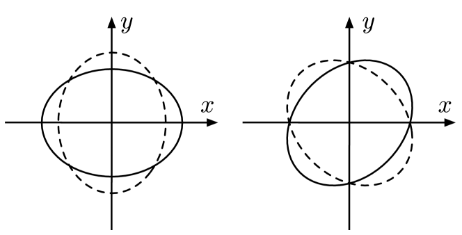
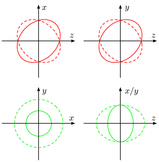
Figure 1: The effect on a ring of free-falling test particles of a gravitational wave in “+” tensor mode (upper left), “$\times$” tensor mode (upper right), “X” vector mode (middle left), “Y” vector mode (middle right), breathing mode (lower left) and longitudinal mode (lower right). In each case the wave is traveling in the $z$-direction. The solid and dotted lines are the states of the ring with a phase difference of $\pi$.

III Methodology

Now consider a network of $D$ gravitational wave detectors labeled by $\alpha=0,\ldots,D-1$, located on the Earth at positions $\vec{r}_{\alpha}$ with respect to a geocentric coordinate system, and producing strain outputs $d_{\alpha}$. A gravitational wave is assumed to originate from a source with sky location $\hat{\Omega}=(\theta,\phi)$, arriving at the geocenter at a time $t$. If only the tensor polarizations are present, one has

$$d_{\alpha}(t+\Delta t_{\alpha})=F_{+,\alpha}(\hat{\Omega})h_{+}(t)+F_{\times,\alpha}(\hat{\Omega})h_{\times}(t)+n_{\alpha}(t+\Delta t_{\alpha}),$$ (2)

where $F_{+,\alpha}$, $F_{\times,\alpha}$ are the beam pattern functions and $n_{\alpha}$ is the noise of detector $\alpha$. The time shifts $\Delta t_{\alpha}$ are given by

$$\Delta t_{\alpha}=\frac{\vec{r}_{\alpha}}{c}\cdot(-\hat{\Omega}).$$ (3)

We can write the $D$-detector observation model more compactly in matrix form:

$$\mathbf{d}=\mathbf{Fh}+\mathbf{n},$$ (4)

where

$$\mathbf{d}=\begin{pmatrix}d_{0}\\ \vdots\\ d_{D-1}\end{pmatrix}\text{,\,\,\,\,\,\,\,}\mathbf{h}=\begin{pmatrix}h_{+}\\ h_{\times}\end{pmatrix}\text{,\,\,\,\,\,\,\,}\mathbf{n}=\begin{pmatrix}n_{0}\\ \vdots\\ n_{D-1}\end{pmatrix},$$ (5)

and

$$\mathbf{F}=\begin{pmatrix}\mathbf{F_{+}}&\mathbf{F_{\times}}\end{pmatrix}=\begin{pmatrix}F_{+,0}&F_{\times,0}\\ \vdots&\vdots\\ F_{+,D-1}&F_{\times,D-1}\end{pmatrix}.$$ (6)

III.1 Null energy

In the above, the gravitational wave signal $\mathbf{s}=\mathbf{F}\mathbf{h}$ can be viewed as being in a subspace of the space of detector outputs spanned by $\mathbf{F_{+}}$ and $\mathbf{F_{\times}}$. We can construct the null projector $\mathbf{P}_{\text{null}}(\hat{\Omega})$ Sutton et al. (2010), which projects away the signal when the projector is constructed with the true sky location. The null projector is given by

$$\mathbf{P}_{\text{null}}=\mathbf{I}-\mathbf{F}_{w}(\mathbf{F}_{w}^{\dagger}\mathbf{F}_{w})^{-1}\mathbf{F}_{w}^{\dagger},$$ (7)

where $\dagger$ denotes Hermitian conjugation and $\mathbf{F}_{w}$ are the noise-weighted beam pattern functions Sutton et al. (2010). If we apply the null projector with the true sky location on the strain data in Eq. (4), we obtain

$$\mathbf{\tilde{z}}(\hat{\Omega}_{\text{true}}) =\mathbf{P}_{\text{null}}(\hat{\Omega}_{\text{true}})\mathbf{\tilde{d}}_{w}$$ (8)

$$=\mathbf{P}_{\text{null}}(\hat{\Omega}_{\text{true}})\mathbf{F}_{w}(\hat{\Omega}_{\text{true}})\mathbf{\tilde{h}}+\mathbf{P}_{\text{null}}(\hat{\Omega}_{\text{true}})\mathbf{\tilde{n}}_{w}$$

$$=\mathbf{P}_{\text{null}}(\hat{\Omega}_{\text{true}})\mathbf{\tilde{n}}_{w}$$

where $\mathbf{\tilde{z}}$ is the null stream which only consists of noise living in a subspace that is orthogonal to the one spanned by $\mathbf{F}_{w,+}$ and $\mathbf{F}_{w,\times}$, and $w$ indicates whitening.

In practice, the data are first whitened before applying the null projector. As in Sutton et al. (2010) we perform the analysis in the time-frequency domain, but using the Wilson-Daubechies-Meyer (WDM) time-frequency transform because of its superior time-frequency localization Necula et al. (2012). The null energy is then defined as Sutton et al. (2010)

$$E_{\text{null}} = \sum_{k}\mathbf{\tilde{z}}_{w}^{\dagger}\mathbf{\tilde{z}}_{w}$$ (9)

$$= \sum_{k}\mathbf{\tilde{d}}_{w}^{\dagger}\mathbf{P}_{\text{null}}^{\dagger}\mathbf{P}_{\text{null}}\mathbf{\tilde{d}}_{w}$$

$$= \sum_{k}\mathbf{\tilde{d}}_{w}^{\dagger}\mathbf{P}_{\text{null}}\mathbf{\tilde{d}}_{w},$$

where $w$ indicates whitening, a tilde refers to the data matrix resulting from the WDM transform, and $\sum_{k}$ sums over the discrete time-frequency pixels. The quantity $E_{\text{null}}$ follows a $\chi^{2}$ distribution with $\text{DoF}=N_{\tau f}(D-2)$ degrees of freedom, where $N_{\tau f}$ is the number of time-frequency pixels used in the analysis.

Now let us assume that there is polarization content in the signal beyond the tensor polarizations. The whitened data matrix can then be written as

$$\tilde{\textbf{d}}_{w}=\textbf{F}_{w,t}{\mathbf{\tilde{h}}}_{t}+\textbf{F}_{w,e}{\mathbf{\tilde{h}}}_{e}+\mathbf{\tilde{n}}_{w},$$ (10)

where the index $t$ is summed over $+$ and $\times$, while the index $e$ is summed over whatever additional polarizations are present. The null energy calculated at the source’s location with pure-tensor beam pattern matrix is given by

$$E_{\textrm{null}} = \sum_{k}\mathbf{\tilde{d}}_{w}^{\dagger}\mathbf{P}_{\textrm{null}}\mathbf{\tilde{d}}_{w}$$ (11)

$$= \sum_{k}\mathbf{\tilde{n}}_{w}^{\dagger}\mathbf{P}_{\textrm{null}}\mathbf{\tilde{n}}_{w}+\sum_{k}\mathbf{\tilde{h}}_{e}^{\dagger}\textbf{F}^{\dagger}_{w,e}\mathbf{P}_{\textrm{null}}\textbf{F}_{w,e^{{}^{\prime}}}\mathbf{\tilde{h}}_{e^{{}^{\prime}}}$$

$$+\sum_{k}2\Re(\mathbf{\tilde{h}}_{e}^{\dagger}\textbf{F}^{\dagger}_{w,e}\mathbf{P}_{\textrm{null}}\mathbf{\tilde{n}}_{w}),$$

where the last two terms signify the presence of the extra polarizations. Next we explain how the $\chi^{2}$ distribution which the null energy would follow in the absence of these additional polarizations, can be used to detect them, in two different ways.

III.2 Null energy method and sky map method

As mentioned before, we assume gravitational wave events with electromagnetic counterpart, so that the true sky position $\hat{\Omega}_{\rm true}$ is known. With the null energy formalism of the previous subsection, this leads to two methods for establishing whether alternative polarizations are present.

• If there are additional polarizations in the signal, then the null energy evaluated at $\hat{\Omega}_{\rm true}$ will no longer follow the $\chi^{2}$ distribution described above. To quantify the size of the deviation, we can assign a p-value to the hypothesis that only tensor polarizations are present, given by

  $$p=\int_{E_{\textrm{null}}}^{\infty}\chi_{\textrm{DoF}}^{2}(x)dx,$$ (12)

  where $E_{\rm null}$ is computed from the detector network data $\mathbf{\tilde{d}}_{w}$ and $\hat{\Omega}_{\rm true}$ assuming the tensor-only hypothesis. Under this null hypothesis, $p$ will be distributed uniformly between 0 and 1. A small p-value would indicate a strong appearance of the additional terms in the right hand side of Eq. (11), suggesting a deviation from GR. In the sequel this method will simply be referred to as the null energy method.

• In the context of null energies, the probability for obtaining particular data $\mathbf{\tilde{d}}_{w}$, given the tensor-only hypothesis $\mathcal{H}_{\rm t}$ and a fiducial sky position $\hat{\Omega}$, can be identified with the probability for the associated null energy:

  $$p(\mathbf{\tilde{d}}_{w}|\hat{\Omega},\mathcal{H}_{\rm t})=\chi^{2}_{\rm DoF}(E_{\rm null}(\mathbf{\tilde{d}}_{w},\hat{\Omega})),$$ (13)

  where $\mathcal{H}_{\rm t}$ enters through the construction of $E_{\rm null}$. Through Bayes’ theorem this likelihood function leads to a posterior density for the sky position:

  $$p(\hat{\Omega}|\mathbf{\tilde{d}}_{w},\mathcal{H}_{\rm t})\propto p(\mathbf{\tilde{d}}_{w}|\hat{\Omega},\mathcal{H}_{\rm t})\,p(\hat{\Omega}|\mathcal{H}_{\rm t}),$$ (14)

  and we let the prior $p(\hat{\Omega}|\mathcal{H}_{\rm t})$ be uniform on the sphere. We can then check for the consistency of the true sky location $\hat{\Omega}_{\rm true}$ with the “sky map” $\mathcal{P}(\hat{\Omega})\equiv p(\hat{\Omega}|\mathbf{\tilde{d}}_{w},\mathcal{H}_{\rm t})$. The point $\hat{\Omega}_{\rm true}$ will fall on the boundary of some $(1-q)$ credible contour on the sphere, where $q$ is given by

  $$q=\int_{\mathcal{P}(\hat{\Omega})\leq\mathcal{P}(\hat{\Omega}_{\textrm{true}})}\mathcal{P}(\hat{\Omega})\,d\hat{\Omega}.$$ (15)

  The quantity $q$ is a p-value for the consistency of $\hat{\Omega}_{\rm true}$ with $\mathcal{P}(\hat{\Omega})$, which under the tensor-only hypothesis is distributed uniformly between 0 and 1. In what follows this method will be referred to as the sky map method.

The two methods are not unrelated. Heuristically, in the null energy method, if $p$ is close to zero then from Eq. (12), $E_{\rm null}(\hat{\Omega}_{\rm true})$ must be large, and in the tail of the chi-square distribution. In that case $\chi^{2}_{\rm DoF}(E_{\rm null}(\hat{\Omega}_{\rm true}))$ will be small, and in the sky map method, through Eqs. (13) and (14), this implies that $\mathcal{P}(\hat{\Omega}_{\rm true})$ is also small. From Eq. (15), the value of $q$ will then be small as well. Generally speaking, when $E_{\rm null}(\hat{\Omega}_{\rm true})$ is an outlier with respect to its distribution under the tensor-only hypothesis, we can expect $\hat{\Omega}_{\rm true}$ to be an outlier with respect to $\mathcal{P}(\hat{\Omega})$, and vice versa. On the other hand, the methods do differ from each other. In the null stream method, the null energy is immediately evaluated at $\hat{\Omega}=\hat{\Omega}_{\rm true}$, so that if the signal happens to have only tensor modes, the value that $E_{\rm null}$ takes is determined only by the noise realization $\mathbf{\tilde{n}}_{w}$ in the detector network. By contrast, in the sky map method we effectively define a likelihood for the full network data $\mathbf{\tilde{d}}_{w}$, which leads to a distribution for the sky position that is then compared with the true one. However, we do not expect major differences in performance: if the signal has strong non-tensorial components, both methods will tend to imply an extreme value of $E_{\rm null}(\hat{\Omega}_{\rm true})$ indicating a departure from the hypothesis that only tensor modes are present.

Both methods allow us to combine information from multiple sources so as to arrive at a stronger statement on the validity of GR, or lack thereof. If GR is an accurate description of the gravitational wave polarization, then the values of $p$ obtained from the null energy method and the values of $q$ obtained using the sky map method should be distributed uniformly between $0$ and $1$. As shown by Fisher Fisher (1970), if one has $N$ samples $\{q_{i}\}$ following a uniform distribution between $0$ and $1$, the test statistic $S$ given by

$$S=-2\sum^{N}_{i=1}\log(q_{i})$$ (16)

follows a $\chi^{2}$ distribution with $2N$ degrees of freedom. Therefore, the combined p-value $p_{\textrm{com}}$ is given by

$$p_{\textrm{com}}=\int_{S}^{\infty}\chi^{2}_{2N}(x)\,dx.$$ (17)

In what follows, we first test the two methods through simulations, and then apply them to the binary neutron star signal GW170817.

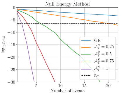
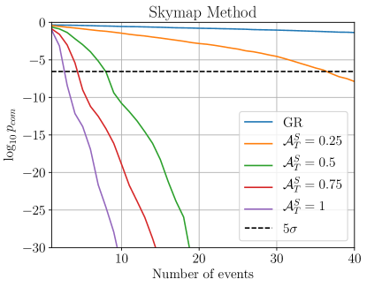
Figure 2: $\log_{10}$ of combined p-values with null energy method (left panel) and skymap method (right panel) against the number of combined events, both for the GR case and for different sets of mock scalar-tensor signals as described in the main text. For all sets of non-GR injections, GR can be rejected at the $5\sigma$ level with a few to a few tens of detections.

IV Simulations, and analyses of GW170817

In this section we evaluate the performance of the null stream and sky map methods by “injecting” simulated signals into synthetic stationary, Gaussian noise following predicted noise power spectral densities for Advanced LIGO and Advanced Virgo at their respective design sensitivities. We take the sources to be zero-spin binary neutron star inspirals with component masses uniformly distributed in $[1,2]\,M_{\odot}$. Positions in the Universe are distributed uniformly in co-moving volume up to distances such that the network signal-to-noise remains above 12, and orientations of the orbital plane are taken to be arbitrary. Binary neutron stars are chosen because of their ability to generate electromagnetic counterparts when they merge, but in principle other transient sources could be considered.

To test the sensitivities of our methods, apart from simulated signals that follow GR we also inject sets of mock scalar-tensor waveforms. The scalar component $h_{S}$ of the latter signals is taken to be

$$h_{S}(t)=\mathcal{A}^{S}_{T}h_{T}(t;\textrm{with a }\pi/4\textrm{ phase shift}),$$ (18)

where $h_{T}$ is the inclination-independent part of the GR polarization $h_{+}$ (i.e. the part that only depends on masses and distance); $\mathcal{A}^{S}_{T}$ can be thought of as including both the inclination dependence of $h_{S}$ and theory-dependent effects that set the intrinsic strength of the scalar component relative to the tensor modes Takeda et al. (2018). The $\pi/4$ phase shift is a strawman for the more general ways in which the scalar component’s phasing might differ from that of the tensor components; in alternative theories of gravity, generically the scalar phase also has a different time dependence Chatziioannou et al. (2012). In each of four sets of scalar-tensor injections, for simplicity we let $\mathcal{A}^{S}_{T}$ take fixed values of 0.25, 0.5, 0.75, or 1.0, effectively taking the inclination dependence of $h_{S}$ to have been averaged over, so that the chosen values for $\mathcal{A}^{S}_{T}$ can be viewed as indicative of the intrinsic strength of the scalar components relative to the tensor modes.

Fig. 2 shows $\log_{10}$ of the combined p-value $p_{\textrm{com}}$ calculated with the null energy method and the sky map method against the number of events. Even for $\mathcal{A}^{S}_{T}=0.25$, it takes only a few tens of detections with electromagnetic counterparts to establish a $5\sigma$ violation of GR. The null energy method appears to be performing slightly better in that it requires fewer sources to attain the $5\sigma$ level, although this could be due to the particular parameter values in our “catalog” of simulated sources. To make more definitive statements a much larger (and computationally costly) simulation campaign would be needed, analyzing many randomly chosen “catalogs” of a few tens of sources each. However, on the basis of Fig. 2 we expect that the difference in performance between the methods will not be very pronounced, so that the one can be used to complement the other.

We note that $p_{\textrm{com}}$ for GR signals gradually approaches the 5$\sigma$ line as the number of events increases; this is because of the systematics in the clustering algorithm used. The largest high-power cluster is consistently selected to be the event candidate, but there is a non-negligible chance for high-power noise pixels to be included in the periphery of the cluster. This happens especially when the burst energy of the signal is not significantly higher than the background noise. The systematic error accumulates as the number of events increases. Hence, when performing analyses for a large number of events, we will have to inject large numbers of simulated GR signals into real noise to obtain a reference or “background” distribution of the test statistic to compare “foreground” results with. This procedure will automatically account for the non-stationary and non-Gaussian nature of detector noise as well as the systematics due to the clustering method. Nevertheless, the results of Fig. 2 are already strongly suggestive of the sensitivities we can expect to attain, given how rapidly $p_{\rm com}$ becomes small in the case of GR violations (note the logarithmic scales on the vertical axes).

These results show that our analysis pipelines are capable of testing for the existence of alternative polarization modes in addition to tensor modes with a 3-detector network. Given a few tens of detections with known sky positions, both methods are sensitive to a scalar component provided that it has appreciable intrinsic strength compared to the tensorial components.

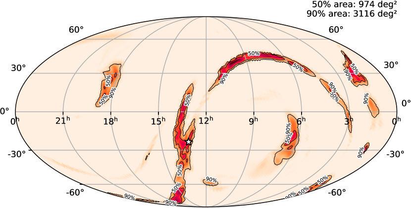
Figure 3: Sky map $\mathcal{P}(\hat{\Omega})$ for GW170817. The star indicates the sky location of the corresponding counterpart SSS17a/AT 2017gfo Abbott et al. (2019b). The sky map is consistent with the counterpart location, which is enclosed in the $50\%$ confidence contour.

A binary neutron star coalescence GW170817 was observed on 17 August 2017 with merger time 12:41:04 UTC (or GPS time 1187008882.4457) Abbott et al. (2017c); LIGO Scientific Collaboration and Virgo Collaboration (2017); Vallisneri et al. (2015). Electromagnetic counterparts were seen, and in particular an optical counterpart was found with very precise localization at right ascension and declination $\alpha=13^{\text{h}}09^{\text{m}}48^{\text{s}}.085\pm 0.018$ and $\delta=-23^{\circ}22^{\prime}53^{\prime\prime}.343\pm 0.218$, respectively Abbott et al. (2017f), which provides us with an opportunity to apply our tests for alternative polarizations. The null energy test yields a p-value of 0.315, while the sky map method gives 0.790; in the latter case, the sky map $\mathcal{P}(\hat{\Omega})$ and true sky location $\hat{\Omega}_{\rm true}$ are shown in Fig. 3. Hence, neither test allows us to reject the tensor-only hypothesis at anything approaching the $5\sigma$ level. (We reiterate that properly speaking the p-values should be compared with a background distribution; this will become important for a larger number of events and smaller p-values.)

V Summary and conclusions

We have introduced two methods to search for polarization modes in addition to the tensor modes, which can be used even with a limited network of detectors (e.g. the two LIGOs and Virgo), though an identifiable electromagnetic counterpart is needed. Both formalisms are based on the notion of null energy. In one case (the null energy test) we use the statistical distribution of the null energy for the given true sky location to compute p-values for the validity of the tensor-only hypothesis. The other method (the sky map test) first leaves the sky location to be free, turning the distribution of null energy into a sky map, for which the consistency with the true sky location can again be quantified in terms of a p-value. Apart from being able to detect mixtures of different polarization modes rather than having to consider purely tensor, purely vector, and purely scalar hypotheses, no waveform models are needed, so that any transient gravitational wave signal can be used in the tests, on condition that the sky position of the source is known.

By injecting mock scalar-tensor signals into synthetic stationary and Gaussian noise, we illustrated how both tests can find scalar contributions at $5\sigma$ confidence with a few tens of signals that have electromagnetic counterparts if the scalar contribution is at least at the 25% level in the sense explained above. Both methods show a slowly accumulating bias towards a GR violation when applied to pure tensor signals, due to the null energy clustering algorithm picking up high-energy noise pixels. Thus there is scope for improvement, although even if tens of signals with counterparts were available today, we would certainly be able to already use either method by constructing a reference distribution for our detection statistic and compare “foreground” results with this “background” distribution.

Finally, we have applied our methods to GW170817, a priori allowing for any mixture of polarizations, but finding p-values that do not induce us to reject the pure-tensor hypothesis.

References

- Aasi et al. (2015) J. Aasi et al. (LIGO Scientific), Class. Quant. Grav. 32, 074001 (2015), arXiv:1411.4547 [gr-qc] .
- Acernese et al. (2015) F. Acernese et al. (VIRGO), Class. Quant. Grav. 32, 024001 (2015), arXiv:1408.3978 [gr-qc] .
- Abbott (2017) B. P. Abbott (2017) pp. 291–311.
- Abbott et al. (2016a) B. P. Abbott et al. (Virgo, LIGO Scientific), Phys. Rev. Lett. 116, 241103 (2016a), arXiv:1606.04855 [gr-qc] .
- Abbott et al. (2016b) B. P. Abbott et al. (Virgo, LIGO Scientific), Phys. Rev. X6, 041015 (2016b), arXiv:1606.04856 [gr-qc] .
- Abbott et al. (2017a) B. P. Abbott et al. (VIRGO, LIGO Scientific), Phys. Rev. Lett. 118, 221101 (2017a), arXiv:1706.01812 [gr-qc] .
- Abbott et al. (2017b) B. P. Abbott et al. (Virgo, LIGO Scientific), Astrophys. J. 851, L35 (2017b), arXiv:1711.05578 [astro-ph.HE] .
- Abbott et al. (2017c) B. P. Abbott, R. Abbott, T. D. Abbott, F. Acernese, et al. (LIGO Scientific Collaboration and Virgo Collaboration), Phys. Rev. Lett. 119, 161101 (2017c).
- Abbott et al. (2017d) B. P. Abbott et al. (Virgo, LIGO Scientific), Phys. Rev. Lett. 119, 141101 (2017d), arXiv:1709.09660 [gr-qc] .
- Abbott et al. (2018a) B. P. Abbott et al. (LIGO Scientific, Virgo), (2018a), arXiv:1811.12907 [astro-ph.HE] .
- Abbott et al. (2020) B. P. Abbott et al. (LIGO Scientific, Virgo), (2020), arXiv:2001.01761 [astro-ph.HE] .
- Abbott et al. (2016c) B. P. Abbott et al. (Virgo, LIGO Scientific), Phys. Rev. Lett. 116, 221101 (2016c), arXiv:1602.03841 [gr-qc] .
- Abbott et al. (2016d) B. P. Abbott et al. (Virgo, LIGO Scientific), Phys. Rev. X6, 041015 (2016d), arXiv:1606.04856 [gr-qc] .
- Abbott et al. (2019a) B. P. Abbott et al. (LIGO Scientific, Virgo), (2019a), arXiv:1903.04467 [gr-qc] .
- Abbott et al. (2018b) B. P. Abbott et al. (LIGO Scientific, Virgo), (2018b), arXiv:1811.00364 [gr-qc] .
- Abbott et al. (2017e) B. P. Abbott et al. (LIGO Scientific, Virgo, Fermi-GBM, INTEGRAL), Astrophys. J. 848, L13 (2017e), arXiv:1710.05834 [astro-ph.HE] .
- Isi and Weinstein (2017) M. Isi and A. J. Weinstein, (2017), arXiv:1710.03794 [gr-qc] .
- Eardley et al. (1973) D. M. Eardley, D. L. Lee, and A. P. Lightman, Phys. Rev. D 8, 3308 (1973).
- Chatziioannou et al. (2012) K. Chatziioannou, N. Yunes, and N. Cornish, Phys. Rev. D 86, 022004 (2012).
- Isi et al. (2015) M. Isi, A. J. Weinstein, C. Mead, and M. Pitkin, Phys. Rev. D91, 082002 (2015), arXiv:1502.00333 [gr-qc] .
- Isi et al. (2017) M. Isi, M. Pitkin, and A. J. Weinstein, Phys. Rev. D96, 042001 (2017), arXiv:1703.07530 [gr-qc] .
- Abbott et al. (2018c) B. P. Abbott et al. (LIGO Scientific, Virgo), Phys. Rev. Lett. 120, 031104 (2018c), arXiv:1709.09203 [gr-qc] .
- Nishizawa et al. (2009) A. Nishizawa, A. Taruya, K. Hayama, S. Kawamura, and M.-a. Sakagami, Phys. Rev. D79, 082002 (2009), arXiv:0903.0528 [astro-ph.CO] .
- Nishizawa et al. (2010) A. Nishizawa, A. Taruya, and S. Kawamura, Phys. Rev. D81, 104043 (2010), arXiv:0911.0525 [gr-qc] .
- Nishizawa and Hayama (2013) A. Nishizawa and K. Hayama, Phys. Rev. D88, 064005 (2013), arXiv:1307.1281 [gr-qc] .
- Callister et al. (2017) T. Callister, A. S. Biscoveanu, N. Christensen, M. Isi, A. Matas, O. Minazzoli, T. Regimbau, M. Sakellariadou, J. Tasson, and E. Thrane, Phys. Rev. X7, 041058 (2017), arXiv:1704.08373 [gr-qc] .
- Abbott et al. (2018d) B. P. Abbott et al. (LIGO Scientific, Virgo), Phys. Rev. Lett. 120, 201102 (2018d), arXiv:1802.10194 [gr-qc] .
- Gürsel and Tinto (1989) Y. Gürsel and M. Tinto, Phys. Rev. D 40, 3884 (1989).
- Wen and Schutz (2005) L. Wen and B. F. Schutz, Gravitational wave data analysis. Proceedings, 9th Workshop, GWDAW 2004, Annecy, France, December 15-18, 2004, Class. Quant. Grav. 22, S1321 (2005), arXiv:gr-qc/0508042 [gr-qc] .
- Ajith et al. (2006) P. Ajith, M. Hewitson, and I. S. Heng, Gravitational wave data analysis. Proceedings, 10th Workshop, GWDAW-10, Brownsville, USA, December 14-17, 2005, Class. Quant. Grav. 23, S741 (2006), arXiv:gr-qc/0604004 [gr-qc] .
- Chatterji et al. (2006) S. Chatterji, A. Lazzarini, L. Stein, P. J. Sutton, A. Searle, and M. Tinto, Phys. Rev. D74, 082005 (2006), arXiv:gr-qc/0605002 [gr-qc] .
- Freise et al. (2009) A. Freise, S. Chelkowski, S. Hild, W. Del Pozzo, A. Perreca, and A. Vecchio, Class. Quant. Grav. 26, 085012 (2009), arXiv:0804.1036 [gr-qc] .
- Regimbau et al. (2012) T. Regimbau et al., Phys. Rev. D86, 122001 (2012), arXiv:1201.3563 [gr-qc] .
- Sutton et al. (2010) P. J. Sutton, G. Jones, S. Chatterji, P. Kalmus, I. Leonor, S. Poprocki, J. Rollins, A. Searle, L. Stein, M. Tinto, and M. Was, New Journal of Physics 12, 053034 (2010), arXiv:0908.3665 [gr-qc] .
- Hayama and Nishizawa (2013) K. Hayama and A. Nishizawa, Phys. Rev. D87, 062003 (2013), arXiv:1208.4596 [gr-qc] .
- Hagihara et al. (2018) Y. Hagihara, N. Era, D. Iikawa, and H. Asada, Phys. Rev. D98, 064035 (2018), arXiv:1807.07234 [gr-qc] .
- Hagihara et al. (2019) Y. Hagihara, N. Era, D. Iikawa, A. Nishizawa, and H. Asada, Phys. Rev. D100, 064010 (2019), arXiv:1904.02300 [gr-qc] .
- Hagihara et al. (2020) Y. Hagihara, N. Era, D. Iikawa, N. Takeda, and H. Asada, Phys. Rev. D101, 041501 (2020), arXiv:1912.06340 [gr-qc] .
- Van Den Broeck (2014) C. Van Den Broeck, in Springer Handbook of Spacetime, edited by A. Ashtekar and V. Petkov (2014) pp. 589–613, arXiv:1301.7291 [gr-qc] .
- Takeda et al. (2018) H. Takeda, A. Nishizawa, Y. Michimura, K. Nagano, K. Komori, M. Ando, and K. Hayama, Phys. Rev. D 98, 022008 (2018), arXiv:1806.02182 [gr-qc] .
- Takeda et al. (2019) H. Takeda, A. Nishizawa, K. Nagano, Y. Michimura, K. Komori, M. Ando, and K. Hayama, Phys. Rev. D 100, 042001 (2019), arXiv:1904.09989 [gr-qc] .
- Aso et al. (2013) Y. Aso et al. (KAGRA), Phys. Rev. D88, 043007 (2013), arXiv:1306.6747 [gr-qc] .
- Iyer et al. (2011) B. Iyer et al., LIGO India, Tech. Rep. LIGO-M1100296 (2011) https://dcc.ligo.org/LIGO-M1100296/public.
- Will (2014) C. M. Will, Living Reviews in Relativity 17, 4 (2014), arXiv:1403.7377 [gr-qc] .
- Necula et al. (2012) V. Necula, S. Klimenko, and G. Mitselmakher, Journal of Physics: Conference Series 363, 012032 (2012).
- Fisher (1970) R. A. Fisher, Statistical methods for research workers. Fourteenth Edition Revised (Oliver and Boyd, 1970).
- Abbott et al. (2019b) B. P. Abbott et al. (LIGO Scientific, Virgo), Phys. Rev. X9, 011001 (2019b), arXiv:1805.11579 [gr-qc] .
- LIGO Scientific Collaboration and Virgo Collaboration (2017) LIGO Scientific Collaboration and Virgo Collaboration, https://www.gw-openscience.org/events/GW170817/ (2017).
- Vallisneri et al. (2015) M. Vallisneri, J. Kanner, R. Williams, A. Weinstein, and B. Stephens, Journal of Physics: Conference Series 610, 012021 (2015).
- Abbott et al. (2017f) B. P. Abbott et al., The Astrophysical Journal 848, L12 (2017f).