Hydrodynamic attractors in phase space

Abstract

Hydrodynamic attractors have recently gained prominence in the context of early stages of ultra-relativistic heavy-ion collisions at the RHIC and LHC. We critically examine the existing ideas on this subject from a phase space point of view. In this picture the hydrodynamic attractor can be seen as a special case of the more general phenomenon of dynamical dimensionality reduction of phase space regions. We quantify this using Principal Component Analysis. Furthermore, we adapt the well known slow-roll approximation to this setting. These techniques generalize easily to higher dimensional phase spaces, which we illustrate by a preliminary analysis of a dataset describing the evolution of a 5-dimensional manifold of initial conditions immersed in a 16-dimensional representation of the phase space of the Boltzmann kinetic equation in the relaxation time approximation.

Introduction– The physics of strong interactions studied in heavy-ion collisions at the RHIC and LHC (see e.g. Ref. Busza:2018rrf for a concise contemporary review) has been a remarkable source of inspiration for the study of complex systems far from equilibrium. The phenomenological success of relativistic hydrodynamics, together with calculations in microscopic models based on holography and kinetic theory, have inspired several novel research directions. One such direction is centered on the notion of hydrodynamic attractors. These were introduced in Ref. Heller:2015dha with the aim of capturing universal features of non-equilibrium physics beyond the limitations of the gradient expansion and were subsequently explored in many works, including Refs. Basar:2015ava ; Aniceto:2015mto ; Romatschke:2017vte ; Spalinski:2017mel ; Strickland:2017kux ; Romatschke:2017acs ; Denicol:2017lxn ; Florkowski:2017jnz ; Behtash:2017wqg ; Casalderrey-Solana:2017zyh ; Blaizot:2017ucy ; Almaalol:2018ynx ; Denicol:2018pak ; Behtash:2018moe ; Spalinski:2018mqg ; Strickland:2018ayk ; Strickland:2019hff ; Blaizot:2019scw ; Jaiswal:2019cju ; Strickland:2019hff ; Kurkela:2019set ; Denicol:2019lio ; Brewer:2019oha ; Behtash:2019qtk ; Chattopadhyay:2019jqj ; Dash:2020zqx ; Shokri:2020cxa ; Almaalol:2020rnu ; Blaizot:2020gql ; Mitra:2020mei ; mazeliauskas2019prescaling .

In the context of reproducing the spectra of soft particles in ultra-relativistic heavy-ion collisions, the underlying observable of interest is the expectation value of the energy-momentum tensor $\langle T^{\mu\nu}\rangle$. Ideally, one would like to have a way of predicting its behaviour as a function of time directly in QCD. Such calculations remain beyond reach, but have been pursued in quantum field theories possessing a gravity dual Maldacena:1997re ; Witten:1998qj ; Gubser:1998bc in a number of works, see Refs. Chesler:2015lsa ; Berges:2020fwq for a review. Another line of development replaces QCD by its effective kinetic theory description Arnold:2002zm , as reviewed in Refs. Schlichting:2019abc ; Berges:2020fwq . The evolution of $\langle T^{\mu\nu}\rangle$ depends on the initial state, captured by the bulk metric in holography, or by the initial distribution function in the kinetic theory. After some time, the vast majority of this information is effectively lost, and $\langle T^{\mu\nu}\rangle$ evolves hydrodynamically. These explorations have led to the idea of a hydrodynamic attractor, identified in Ref. Heller:2015dha in a class of hydrodynamic theories Muller:1967zza ; Israel:1979wp ; Baier:2007ix as a specific solution which is approached by generic solutions initialized at arbitrarily small times. It was also observed there that a “slow-roll” condition akin to what is used in inflationary cosmology Liddle:1994dx ; Spalinski:2007kt leads to an accurate approximation of this attractor. Subsequent works have lead to many interesting phenomenological applications Heller:2015dha ; Romatschke:2017vte ; Behtash:2018moe ; Giacalone:2019ldn ; Dore:2020fiq .

Despite these developments, there are three important yet largely unexplored issues. The first addresses the different concepts of attractor, the second concerns their relevance for the dynamics of initial states of interest and the third is the question of their existence beyond highly-symmetric settings. We address these points with the goal of clearing the ground for new developments, in particular for generalisations to more realistic flows with less symmetry. Our approach is based on the phase space picture, i.e., the space of variables needed to parametrize the dynamics underlying $\langle T^{\mu\nu}\rangle$, which was introduced in this context in Refs. Behtash:2017wqg ; behtash2019global .

Dissipation of initial state information– There are two key features of the dynamics following an ultra-relativistic heavy-ion collision: the expansion which drives the system away from equilibrium and interactions which favour equilibration Blaizot:2017ucy . The simplest model of this is Bjorken flow which assumes one-dimensional expansion and boost-invariance along the expansion axis, conveniently described in terms of proper time $\tau$ and spacetime rapidity $y$. In interacting conformal theories, at asymptotically late times the system follows a scaling solution for the (effective) temperature Bjorken:1982qr

$$T(\tau)=\frac{\Lambda}{(\Lambda\tau)^{1/3}}+\dots~{}.$$ (1)

In this equation, the dimensionful constant $\Lambda$ is the only trace of initial conditions. Corrections to this come in two forms: higher-order power-law terms which are sensitive only to $\Lambda$, and exponential corrections which encode information about the initial conditions and describe its dissipation  Janik:2006gp ; Heller:2013fn ; Heller:2015dha ; Casalderrey-Solana:2017zyh ; Aniceto:2015mto ; Aniceto:2018uik . This asymptotic form is usually referred to as a transseries Aniceto:2018bis . The simplest models where this can be observed explicitly are formulated in the language of hydrodynamics.

Models of hydrodynamics– We primarily focus on hydrodynamic theories (see Ref. Florkowski:2017olj for a review), which despite their name include transient non-hydrodynamic excitations needed to avoid acausality. In such models, $\langle T^{\mu\nu}\rangle$ is decomposed into a perfect fluid term and a “dissipative” part denoted by $\pi^{\mu\nu}$:

$$\langle T^{\mu\nu}\rangle=({\cal E}+{\cal P})\,u^{\mu}u^{\nu}+{\cal P}\,g^{\mu\nu}+\pi^{\mu\nu},$$ (2)

where $u_{\mu}u^{\mu}=-1$, $u_{\mu}\pi^{\mu\nu}=0$, and the energy density $\cal E$ and pressure $\cal P$ are related by the thermodynamic equation of state. In the conformal case considered here, ${\cal P}=\frac{\cal E}{3}$. Conservation equations of $\langle T^{\mu\nu}\rangle$ provide the four equations of motion for $\cal E$ and $u^{\mu}$. Hydrodynamic models, building on the original ideas of Refs. Muller:1967zza ; Israel:1979wp , provide the remaining equations for $\pi^{\mu\nu}$ in terms of relaxation-type dynamics that ensure matching to the hydrodynamic gradient expansion of any microscopic model.

In this Letter, we consider two classes of models. The first one is the Müller-Israel-Stewart (MIS) model Muller:1967zza ; Israel:1979wp

$$\tau_{\pi}\,{\cal D}\,\pi^{\mu\nu}=-\pi^{\mu\nu}+\eta\,\sigma^{\mu\nu},$$ (3)

where ${\cal D}\,\pi^{\mu\nu}\equiv u^{\alpha}\nabla_{\alpha}\pi^{\mu\nu}+\ldots$ is the Weyl-covariant derivative in the co-moving direction Loganayagam:2008is ; Heller:2014wfa and $\sigma^{\mu\nu}=2\,{\cal D}^{(\mu}u^{\nu)}$ is the shear tensor. One can supplement Eq. (3) with additional terms defining the so-called Baier-Romatschke-Son-Starinets-Stephanov (BRSSS) model Baier:2007ix and in the following we will refer to it as MIS/BRSSS. Conformal symmetry requires that

$$\eta=C_{\eta}\frac{{\cal E}+{\cal P}}{T}\quad\mathrm{and}\quad\tau_{\pi}=\frac{C_{\tau_{\pi}}}{T}\quad\mathrm{with}\quad{\cal E}\sim T^{4},$$ (4)

where $C_{\eta}$, $C_{\tau_{\pi}}$ are dimensionless constants and $T$ is defined as the temperature of an equilibrium state at the same energy density $\cal E$. Eq. (3) implies relaxation phenomena on a time scale defined by the relaxation time $\tau_{\pi}$.

For the Bjorken flow, the combined equations reduce to a second order ordinary differential equation (ODE) for the effective temperature $T(\tau)$, see Eq. (7.17) in Ref. Florkowski:2017olj . The hydrodynamic attractor was originally observed in this model in Ref. Heller:2015dha using a special scale-invariant parametrization involving pressure anisotropy (note $\pi^{2}_{\,2}=\pi^{3}_{\,3}$)

$${\cal A}=\frac{\pi^{2}_{\,2}-\pi^{y}_{\,y}}{{\cal P}}=6+18\,\tau\,\frac{\dot{T}(\tau)}{T(\tau)}$$ (5)

understood as a function of time measured by

$$w=\tau\,T(\tau)~{}.$$ (6)

We denote derivatives with respect to $\tau$ with a dot and derivatives with respect to $w$ with a prime. In contrast with $T(\tau)$, ${\cal A}(w)$ satisfies a first order ODE, see Eq. (7.18) in Ref. Florkowski:2017olj .

The second hydrodynamic theory of interest here is the Heller-Janik-Spalinski-Witaszczyk (HJSW) model Heller:2014wfa (see also Ref. Noronha:2011fi ), in which Eq. (3) is replaced by

$$\big{\{}(\frac{1}{T}{\cal D})^{2}+\frac{2}{T^{2}\tau_{\pi}}{\cal D}\big{\}}\pi^{\mu\nu}=-\frac{\tau_{\pi}^{-2}+\omega^{2}}{T^{2}}\big{\{}\pi^{\mu\nu}+\eta\sigma^{\mu\nu}\big{\}}.$$ (7)

This structure again ensures relaxation phenomena on a time scale $\tau_{\pi}$, but here they occur in an oscillatory manner as in ${\mathcal{N}}=4$ supersymmetric Yang-Mills theory Kovtun:2005ev , with frequency $\omega=C_{\omega}T$. This model leads to a third order ODE for the effective temperature $T(\tau)$ or a second order ODE for ${\cal A}(w)$, see Eq. (7.26) in Ref. Florkowski:2017olj , and provides a workable setting with a richer set of initial conditions than offered by MIS/BRSSS.

Hydrodynamic attractors– The hydrodynamic attractor in MIS/BRSSS arose through studying a range of solutions for ${\cal A}(w)$ which converge and then evolve toward local thermal equilibrium Heller:2015dha . This behaviour is known in the mathematical literature kloeden2011nonautonomous as a forward attractor. Intuitively, forward attractors are solutions that attract nearby sets as $w\rightarrow\infty$. In MIS/BRSSS every solution is a forward attractor. Conversely, by considering solutions initialized at earlier and earlier times we observe that generic solutions (which diverge at $w=0$) decay to a specific solution which is regular there. Such behaviour is known as a pullback attractor.

These two notions of attractors, introduced in this context in behtash2019global are concerned with different regimes: the forward attractor describes asymptotically late times while the pullback attractor is a statement about early times. In MIS/BRSSS there is a unique solution which is both a pullback attractor and a forward attractor; we denote this solution by ${\cal A}_{\star}(w)$.

Attractors and phase space– The above discussion raises two concerns. The first is that were one to visualize a range of solutions $T(\tau)$, the hydrodynamic attractor would not be apparent, and yet it is encoded there since $\mathcal{A}(w)$ can be clearly derived from $T(\tau)$. If a different observable showed attractor behaviour how would one find it? This issue must be clarified if one aims to identify attractors in more complicated settings. We address it by considering the full phase space parameterised by $(\tau,T,\dot{T})$ for MIS/BRSSS and $(\tau,T,\dot{T},\ddot{T})$ for HJSW. We include proper time as one of the phase space variables because we are dealing with a non-autonomous system.

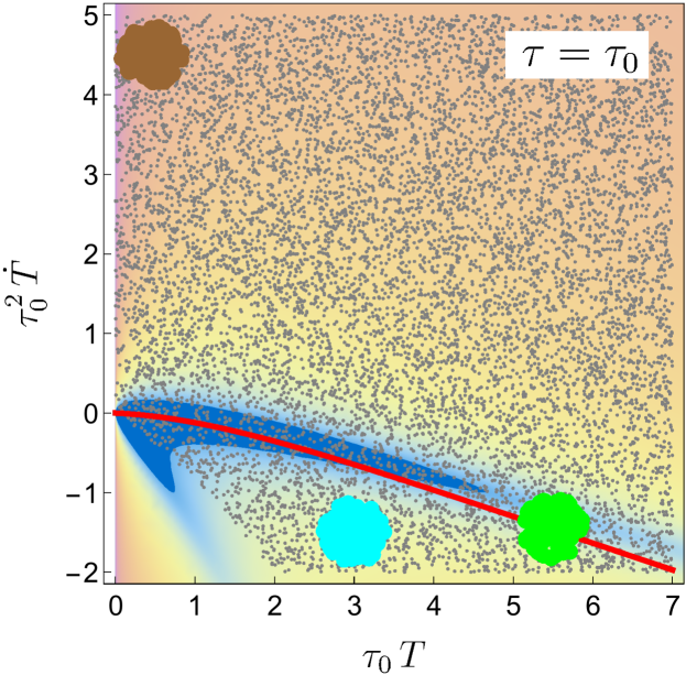
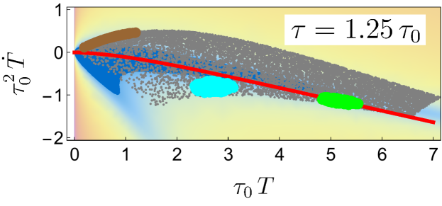
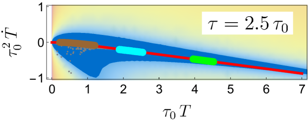
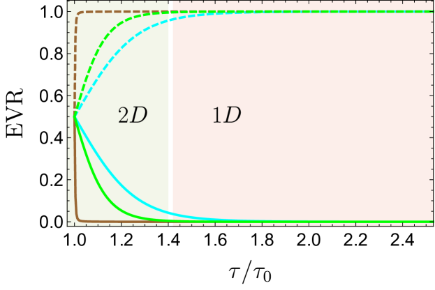
The second concern stems from the fact that forward and pullback attractors strongly depend on either asymptotically late or asymptotically early time dynamics. Such asymptotic regimes may be inaccessible or unphysical. We address this by focusing on the local dynamics on families of constant-$\tau$ slices of phase space, on which solutions of the equations of motion appear as points (see Figs. 1 and 3). However, any particular solution ${\cal A}(w)$ corresponds to a different curve on each slice, as dictated by Eq. (5). On the basis of earlier studies one expects that as $\tau$ increases, different solutions (points on constant-$\tau$ slices) will collapse to the curves representing the attractor ${\cal A}_{*}(w)$. This is what one eventually sees in Figs. 1 (bottom) and 3 (bottom-right), but numerical studies of phase space histories reveal a much finer picture. The process of information loss occurs in three phases: local dimensionality reduction, approach to the hydrodynamic attractor loci (red curves in Fig. 1), and evolution toward equilibrium along the attractor. Consider a finite “cloud” of initial states, such as any one of the three colored sets of points shown in Fig. 1. Each cloud contracts and becomes one-dimensional. When this happens depends on the initial conditions. For example, the brown cloud in Fig. 1 (the one initialized at smallest value of $\tau_{0}T$) loses a dimension quite early and rather far from the attractor, while the other two do this much later.

Figure 1: Three snapshots of evolution in MIS/BRSSS phase space of a cloud of about 10,000 random states in the region determined by the ranges of the top plot. The red curve denotes the family of solutions corresponding to the attractor ${\cal A}_{\star}(\tau\,T)$. The background color represents the speed at which the points move in phase space, with magenta being faster than blue according to the velocity defined in the text. The dark blue denotes the slow region beyond the color coding scale. For the purposes of visualizing local dimensionality reduction, see also Fig. 2, we track three initially spherical regions. The plots were made for $C_{\eta}=0.75$ and $C_{\tau_{\pi}}=1$, see Eqns. (3) and (4), and $\tau_{0}$ denotes initialization time.

Quantifying dimensionality reduction– We have argued that dimensionality reduction in phase space is an important feature of hydrodynamic attractors, but so far we have not provided a working recipe to quantify this process. A promising direction, which we only begin to explore here, follows from recognizing that dimensionality reduction is one of the basic tasks of machine learning. For the simple cases considered here, Principal Component Analysis (PCA) is quite effective (see Refs. Bhalerao:2014mua ; Mazeliauskas:2015efa ; Bozek:2017thv ; Liu:2019jxg ; Gardim:2019iah for other applications of PCA to problems in ultra-relativistic heavy-ion collisions). Intuitively, PCA quantifies the variations of a data set in different directions and associates an explained variance with each of them.

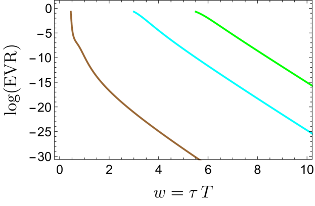
We start by applying PCA to the two-dimensional phase space of MIS/BRSSS. On the initial time slice we pick a state $(T,\dot{T})$ and consider a random set of points within a disc around it. For this set of points, the two principal components are approximately equal in magnitude. At each timestep we recompute the principal components for the set of states we started with (see Fig. 1) and their evolution in time is shown in Fig. 2. Dimensionality reduction is signalled when one of the components is much smaller than the other one.

Figure 2: Top: Evolution of explained variance ratio of each principal component in MIS/BRSSS for circles (radius: $10^{-4}$) of initial conditions with centres lying in the middle of initial dots of corresponding color in Fig. 1. Bottom: For large enough values of $w$ there is an exponential decay with a decay rate consistent with twice the transient mode contribution to ${\cal A}(w)$. The initial dimensional reduction of the brown region we view as triggered by the expansion rather than by nonhydrodynamic mode decay Kurkela:2019set .

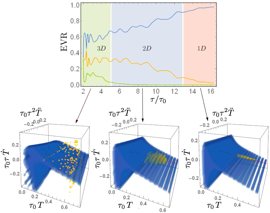
This analysis extends to phase spaces of arbitrary dimension. An interesting example is provided by the three-dimensional phase space of HJSW. The evolution of principal components is shown in the upper part of Fig. 3. There are three stages of dimensionality reduction. The first, from three to two dimensions, is analogous to the earliest phase of the collapse in MIS/BRSSS, most likely due to the expansion. The second stage is characterized by oscillations typical of the non-hydrodynamic sector of HJSW. These eventually dissipate resulting in the final stage of one-dimensional evolution.

Slow-roll in phase space– The basic intuition is that the attractor locus should correspond to a region where the flow in phase space is slowest. One way to motivate why the slow region should behave as an attractor is to use an argument inspired by thermodynamics: a system is likely to be found in a large entropy macrostate because such states cover the majority of phase space. In our setting, the system is likely to be in a slow region because it takes a long time to escape it, while the fast regions can be quickly traversed.

We have found that in the case of MIS/BRSSS this idea correctly identifies the attractor on any given time slice. Let $\vec{X}(\tau)=\left(\tau_{0}\,T(\tau),\tau_{0}^{2}\,\dot{T}(\tau)\right)$ be a point in a slice of phase space at time $\tau$ and $\tau_{0}$ denotes initialization time. This point moves with velocity $\vec{V}=\tau_{0}\dot{\vec{X}}(\tau)$. The slow region is defined by its Euclidean norm $V$, which has a minimum at asymptotically late times when the system approaches local thermal equilibrium. However, the whole region where it is small is of dynamical significance. In Fig. 1, the background color is determined by $V$, where bluer color implies lower speed. There is a slow region stretching out from local thermal equilibrium, and the attractor $\mathcal{A}_{*}(w)$ lies along it. It can be approximated by a slow-roll approximation Heller:2015dha where one neglects $\ddot{T}$ in the equations of motion. This generalizes directly to phase spaces of any dimension. For the case of HJSW the slow regions are shown also in blue in the bottom row of Fig. 3.

In non-autonomous systems the slow region changes with time. If it were to evolve faster than the solutions do, it would not be useful to characterize the attractor. This is however not the case here: in both Fig. 1 and Fig. 3 we observe that once solutions reach the slow-region, they stay inside and evolve with it. This is analogous to the adiabatic evolution observed in the case of the Boltzmann equation in the relaxation time approximation considered in Ref. Brewer:2019oha .

Figure 3: In HJSW, the evolution of a cloud in phase space can be split into three stages, corresponding to the dimensionality of the cloud. The reduction from three to two dimensions corresponds to a collapse onto the slow region (blue region in plots). The plots were made with $C_{\eta}=0.75$, $C_{\tau_{\pi}}=1.16$ and $C_{\omega}=9.8$.

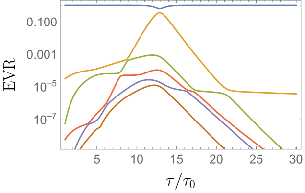
Multidimensional phase spaces– In realistic settings, one may not be able to consider the full phase space, but only some finite-dimensional, approximate representation thereof. As an example of such a procedure, we have studied a $16$-dimensional subspace of the phase space of the Boltzmann kinetic equation in the relaxation time approximation Baym:1984np ; Florkowski:2013lya . This subspace is captured by taking the lowest $16$ moments of the distribution function and solving the evolution equations as in Ref. Strickland:2018ayk ; Strickland:2019hff . We followed the evolution of a set of 240 initial conditions spanning a $5$-dimensional manifold embedded in the $16$-dimensional phase. The results of an exploratory analysis of the resulting dataset using PCA are illustrated by Fig. 4 and described in more detail in the Supplementary Material . This preliminary study supports the viability of the proposed approach in multidimensional phase spaces.

Figure 4: The six largest principal components and their explained variance ratios as a function of $\tau$. Due to the bias in initial conditions, one component dominates already at the initial time. This direction is not dynamically preferred, as the other components initially grow in importance and only at $\tau\approx 15\,\tau_{0}$ we see their expected exponential decay. At $\tau\approx 22\,\tau_{0}$, the second principal component stabilizes. This feature may reflect the limitations of PCA to capture effects of curved regions in phase space.

Summary and outlook– The pressure anisotropy ${\cal A}(w)$ has been observed to exhibit universal behaviour in various models, characterized by different authors in terms of concepts such as pullback/forward attractors or slow-roll, all of which capture some aspects information loss in dissipative systems. In this work we have described hydrodynamic attractors using concepts which allow for generalizations to more realistic settings. We have shown that this can be achieved by considering the phase space of the theory, which alleviates the need to know in advance which particular quantity makes attractor behaviour manifest. From this perspective, the hydrodynamic attractor is associated with the more general notion of dimensionality reduction of phase space regions.

Acknowledgements– We thank J. Carrasquilla, R. Janik, D. Teaney as well as participants of the XIV Polish Workshop on Relativistic Heavy-Ion Collisions at AGH, Initial Stages 2019 at Columbia University and Foundational Aspects of Relativistic Hydrodynamics at Banff International Research Station where this work was presented at different stages of development for helpful discussions. The Gravity, Quantum Fields and Information group at AEI is supported by the Alexander von Humboldt Foundation and the Federal Ministry for Education and Research through the Sofja Kovalevskaja Award. MS was supported by the Polish National Science Centre grant 2018/29/B/ST2/02457.

Supplemental Material: Hydrodynamic attractors in phase space

I Dimensionality reduction in Kinetic theory

As a test of our approach in a somewhat more realistic example, we present some details of its application to the dynamics of kinetic theory, specifically the Boltzmann equation in the relaxation time approximation (RTA). This setting was examined in the context of attractors in a number of recent papers Romatschke:2017vte ; Romatschke:2017acs ; Kurkela:2019set . Most relevant for us is the work of Strickland Strickland:2018ayk ; Strickland:2019hff , who considered the dynamics of the moments of the distribution function and demonstrated that they too show attractor behaviour. In this work we study the same collection of moments but instead of considering each of them separately, we view them as coordinates on a truncated phase space. From this perspective one apply the approach proposed in this Letter to identify correlations between moments and determine the effective dimensionality of a set of solutions as it evolves.

In RTA kinetic theory, in boost-invariant flow, the distribution function satisfies Baym:1984np ; Florkowski:2013lya

$$f(\tau,u,p_{T})=D(\tau,\tau_{0})f_{0}(u,p_{T})\\ +\int_{\tau_{0}}^{\tau}\frac{d\tau^{\prime}}{\tau_{\text{eq}}(\tau^{\prime})}D(\tau,\tau^{\prime})f_{\text{eq}}(\tau^{\prime},u,p_{T}),$$ (S1)

where $f_{0}$ defines the initial conditions. $u,\tau$ and $p_{T}$ are boost invariant variables and it is convenient to define $v\equiv\sqrt{u^{2}+p_{T}^{2}\tau^{2}}$. The moments of the distribution function are defined by

$$M^{nm}[f]\equiv\int\frac{du}{v}d^{2}p_{T}\left(\frac{v}{\tau}\right)^{n}\left(\frac{u}{\tau}\right)^{m}f.$$ (S2)

We follow Ref. Strickland:2018ayk ; Strickland:2019hff closely in solving for the evolution of moments. Each moment satisfies

$$M^{nm}(\tau)=D(\tau,\tau_{0})M^{nm}[f_{0}](\tau)\\ +\int_{\tau_{0}}^{\tau}\frac{d\tau^{\prime}}{\tau_{\text{eq}}(\tau^{\prime})}D(\tau,\tau^{\prime})M^{nm}[f_{\text{eq}}](\tau^{\prime})~{}.$$ (S3)

For an equilibrium distribution of the Boltzmann form

$$f_{\text{eq}}(\tau,u,p_{T})=e^{-\frac{v}{T(\tau)\tau}},$$ (S4)

each $M^{nm}[f_{\text{eq}}]$ can be calculated analytically and are determined by $T(\tau)$. The temperature is related to the energy density by Landau matching and it follows that the equation for $M^{20}$ translates into a closed equation for the temperature

$$T^{4}(\tau)=D(\tau,\tau_{0})T^{4}[f_{0}](\tau)\\ +\int_{\tau_{0}}^{\tau}\frac{d\tau^{\prime}}{2\tau_{\text{eq}}(\tau^{\prime})}D(\tau,\tau^{\prime})T^{4}(\tau^{\prime})H\left(\frac{\tau^{\prime}}{\tau}\right),$$ (S5)

where $H(y)=y^{2}+\frac{\tan^{-1}\left(\sqrt{\frac{1}{y^{2}}-1}\right)}{\sqrt{\frac{1}{y^{2}}-1}}$. Solving this equation for $T(\tau)$ allows one to calculate every moment $M^{nm}(\tau)$. As in the main text of our Letter, we consider a conformal theory with

$$T\tau_{\text{eq}}=5\eta/s$$ (S6)

and we take $\eta/s=1/(4\pi)$. The scaled moments

$$\bar{M}^{nm}(\tau)=M^{nm}(\tau)/M^{nm}_{\text{eq}}(\tau),$$ (S7)

which all tend to unity at equilibrium, provide a natural setting in which to study phase space dimensionality reduction in this model. This space is infinite-dimensional but as in Refs. Strickland:2018ayk ; Strickland:2019hff we direct our attention to the 16 moments with $n$ and $m\leq 3$.

At large $\tau$ the effective temperature evolves according to the Bjorken asymptotics (see Eq. (1)) up to exponentially decaying corrections which reflect the spectrum of non-hydrodynamic modes Heller:2016rtz ; Heller:2018qvh . Given the time evolution of individual moments Strickland:2018ayk ; Strickland:2019hff , within the phase space picture we expect that a single principal component dominates the late time signal, while the rest should decay exponentially.

Figure S1: The derivative of the logarithm of the explained variances seems to approach a constant at large $w$, indicating an exponential decay. All the components have a similar decay rate, showing that the collapse is somewhat uniform. As was observed in BRSSS (see Fig. 2 in the main text), this decay rate is consistent with twice the decay rate of the non-hydrodynamic modes (dashed magenta line). The oscillations whose frequency decreases at later times is also a feature shared by the non-hydrodynamic modes, see Eq. (S8).

Defining the dimensionless time variable $w\equiv\tau/\tau_{\text{eq}}$ (the normalization of this variable differs by a constant factor from what is used in the main text), the behaviour is even simpler. The power law piece of different solutions becomes universal and the difference between two solutions at late times is to leading order

$$\delta M^{nm}\sim e^{-\frac{3}{2}w}w^{\beta},$$ (S8)

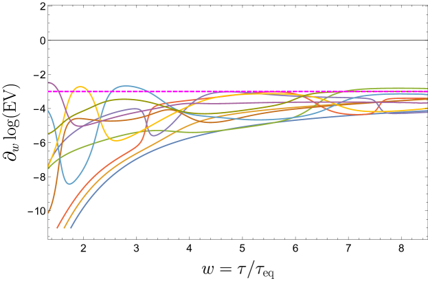
where $\beta$ is a certain set of complex numbers Heller:2018qvh . Thus, applying PCA to the set of solutions as a function of $w$, the expectation is that all of them decay exponentially with the same rate asymptotically. Note also that the imaginary part of $\beta$ leads to oscillations in logarithmic time.

We choose as our family of initial conditions

$$f_{0}(u,p_{T})=A(T_{0})e^{-\frac{\sqrt{u^{2}/\alpha_{0}^{2}+p_{T}^{2}\tau_{0}^{2}}}{\Lambda_{0}\tau_{0}}}\lvert u\rvert^{c_{u}}\lvert p_{T}\rvert^{c_{p}},$$ (S9)

where $A(T_{0})$ is a normalization factor ensuring that the initial temperature is $T_{0}$. These initial conditions depend on five parameters $(T_{0},\Lambda_{0},\alpha_{0},c_{u},c_{p})$. For these initial conditions, it is easy to evaluate $M^{nm}[f_{0}]$ to arbitrary precision. This is the reason why they were used earlier in Ref. Heller:2018qvh to explore hydrodynamization patterns in kinetic theory. Sampling these five parameters at the initial point in time leads to an, at most, five-dimensional manifold embedded in a 16-dimensional space. We sample uniformly in (0.8-1.2 GeV, 0.8-1.2 GeV, 0.5-1.4, -0.5-1, -0.5-1) and take $\tau_{0}=0.1$ fm/c.

In the BRSSS and HJSW models to which most of the main text was devoted, we had much more control over initial conditions and could choose them without bias in any particular direction. The explained variances were initially equal and the hierarchy that developed was purely a result of the dynamics. The present case is more challenging, as the initial conditions we use have a built in bias which translates into a hierarchy of explained variances already at the initial time. Nevertheless, the evolution exhibits the expected characteristics of dimensionality reduction also in this restricted setting. In Fig. 4 in the main text, we plot the explained variance ratio of the six largest principal components as a function of $\tau$. At early times, the bias in initial conditions is the reason for the large difference in explained variance. As time elapses, the relative importance of the smaller ones grow quickly, showing that the initial situation was not dynamically preferred. At $\tau\approx 15\,\tau_{0}$, dimensionality reduction occurs leaving a single dominant component while the rest decays exponentially. Surprisingly, at $\tau\approx 22\,\tau_{0}$, the second component stabilizes, albeit at a very small value. We conjecture that this is due to the inherent limitations of PCA to capture curved manifolds. If the curve corresponding to the hydrodynamic modes has curvature, more principal components will be needed to describe it, resulting in the behaviour we see in the figure. It would be interesting to apply more sophisticated data analysis methods that can capture such non-linearity, e.g. kernel-PCA.

To characterize the decay rate, we use PCA on the solutions as a function of $w$. In Fig. S1 we plot the derivative of the logarithm of the explained variances. At large $w$, they seem to saturate to a constant which is consistent with the twice the decay rate of the non-hydrodynamic modes. In addition, at earlier times we see oscillations, whose frequency seem to decrease at later times. This strengthens the connection to the non-hydrodynamic modes, which exhibit oscillations in logarithmic time.

We have demonstrated that PCA can be used to study the dynamics of dimensionality reduction in theories with higher dimensional phase spaces. While kinetic theory is in fact infinite-dimensional, all of this information will never be physically relevant and one may truncate the to a finite dimensional space (in this case, the lower moments of the distribution function). At late times, when the dimensionality reduction is governed by interactions, we can interpret the evolution of explained variances in terms of hydrodynamic and non-hydrodynamic modes. At earlier times, when the expansion is dominant, the character of the collapse will be different Kurkela:2019set . We leave this analysis to future work.

References

- (1) W. Busza, K. Rajagopal and W. van der Schee, Heavy Ion Collisions: The Big Picture, and the Big Questions, Ann. Rev. Nucl. Part. Sci. 68 (2018) 339–376 [arXiv:1802.04801].
- (2) M. P. Heller and M. Spaliński, Hydrodynamics Beyond the Gradient Expansion: Resurgence and Resummation, Phys. Rev. Lett. 115 (2015), no. 7 072501 [arXiv:1503.07514].
- (3) G. Başar and G. V. Dunne, Hydrodynamics, resurgence, and transasymptotics, Phys. Rev. D92 (2015), no. 12 125011 [arXiv:1509.05046].
- (4) I. Aniceto and M. Spaliński, Resurgence in Extended Hydrodynamics, Phys. Rev. D93 (2016), no. 8 085008 [arXiv:1511.06358].
- (5) P. Romatschke, Relativistic Fluid Dynamics Far From Local Equilibrium, Phys. Rev. Lett. 120 (2018), no. 1 012301 [arXiv:1704.08699].
- (6) M. Spaliński, On the hydrodynamic attractor of Yang–Mills plasma, Phys. Lett. B776 (2018) 468–472 [arXiv:1708.01921].
- (7) M. Strickland, J. Noronha and G. Denicol, The anisotropic non-equilibrium hydrodynamic attractor, arXiv:1709.06644.
- (8) P. Romatschke, Relativistic Hydrodynamic Attractors with Broken Symmetries: Non-Conformal and Non-Homogeneous, JHEP 12 (2017) 079 [arXiv:1710.03234].
- (9) G. S. Denicol and J. Noronha, Analytical attractor and the divergence of the slow-roll expansion in relativistic hydrodynamics, arXiv:1711.01657.
- (10) W. Florkowski, E. Maksymiuk and R. Ryblewski, Coupled kinetic equations for quarks and gluons in the relaxation time approximation, arXiv:1710.07095.
- (11) A. Behtash, C. N. Cruz-Camacho and M. Martinez, Far-from-equilibrium attractors and nonlinear dynamical systems approach to the Gubser flow, Phys. Rev. D97 (2018), no. 4 044041 [arXiv:1711.01745].
- (12) J. Casalderrey-Solana, N. I. Gushterov and B. Meiring, Resurgence and Hydrodynamic Attractors in Gauss-Bonnet Holography, JHEP 04 (2018) 042 [arXiv:1712.02772].
- (13) J.-P. Blaizot and L. Yan, Fluid dynamics of out of equilibrium boost invariant plasmas, arXiv:1712.03856.
- (14) D. Almaalol and M. Strickland, Anisotropic hydrodynamics with a scalar collisional kernel, Phys. Rev. C97 (2018), no. 4 044911 [arXiv:1801.10173].
- (15) G. S. Denicol and J. Noronha, Hydrodynamic attractor and the fate of perturbative expansions in Gubser flow, Phys. Rev. D99 (2019), no. 11 116004 [arXiv:1804.04771].
- (16) A. Behtash, S. Kamata, M. Martinez and C. N. Cruz-Camacho, Non-perturbative rheological behavior of a far-from-equilibrium expanding plasma, arXiv:1805.07881.
- (17) M. Spaliński, Universal behaviour, transients and attractors in supersymmetric Yang–Mills plasma, Phys. Lett. B784 (2018) 21–25 [arXiv:1805.11689].
- (18) M. Strickland, The non-equilibrium attractor for kinetic theory in relaxation time approximation, JHEP 12 (2018) 128 [arXiv:1809.01200].
- (19) M. Strickland and U. Tantary, Exact solution for the non-equilibrium attractor in number-conserving relaxation time approximation, arXiv:1903.03145.
- (20) J.-P. Blaizot and L. Yan, Emergence of hydrodynamical behavior in expanding quark-gluon plasmas, arXiv:1904.08677.
- (21) S. Jaiswal, C. Chattopadhyay, A. Jaiswal, S. Pal and U. Heinz, Exact solutions and attractors of higher-order viscous fluid dynamics for Bjorken flow, arXiv:1907.07965.
- (22) A. Kurkela, W. van der Schee, U. A. Wiedemann and B. Wu, Early- and Late-Time Behavior of Attractors in Heavy-Ion Collisions, Phys. Rev. Lett. 124 (2020), no. 10 102301 [arXiv:1907.08101].
- (23) G. S. Denicol and J. Noronha, Exact hydrodynamic attractor of an ultrarelativistic gas of hard spheres, arXiv:1908.09957.
- (24) J. Brewer, L. Yan and Y. Yin, Adiabatic hydrodynamization in rapidly-expanding quark-gluon plasma, arXiv:1910.00021.
- (25) A. Behtash, S. Kamata, M. Martinez and H. Shi, Global flow structure and exact formal transseries of the Gubser flow in kinetic theory, arXiv:1911.06406.
- (26) C. Chattopadhyay and U. W. Heinz, Hydrodynamics from free-streaming to thermalization and back again, Phys. Lett. B801 (2020) 135158 [arXiv:1911.07765].
- (27) A. Dash and V. Roy, Hydrodynamic attractors for Gubser flow, arXiv:2001.10756.
- (28) M. Shokri and F. Taghinavaz, Bjorken flow in the general frame and its attractor, arXiv:2002.04719.
- (29) D. Almaalol, A. Kurkela and M. Strickland, Non-equilibrium attractor in high-temperature QCD plasmas, arXiv:2004.05195.
- (30) J.-P. Blaizot and L. Yan, Analytical attractor for Bjorken expansion, arXiv:2006.08815.
- (31) T. Mitra, S. Mondkar, A. Mukhopadhyay, A. Rebhan and A. Soloviev, Hydrodynamic attractor of a hybrid viscous fluid in Bjorken flow, arXiv:2006.09383.
- (32) A. Mazeliauskas and J. Berges, Prescaling and far-from-equilibrium hydrodynamics in the quark-gluon plasma, Physical review letters 122 (2019), no. 12 122301.
- (33) J. M. Maldacena, The Large N limit of superconformal field theories and supergravity, Adv.Theor.Math.Phys. 2 (1998) 231–252 [arXiv:hep-th/9711200].
- (34) E. Witten, Anti-de Sitter space and holography, Adv.Theor.Math.Phys. 2 (1998) 253–291 [arXiv:hep-th/9802150].
- (35) S. Gubser, I. R. Klebanov and A. M. Polyakov, Gauge theory correlators from noncritical string theory, Phys.Lett. B428 (1998) 105–114 [arXiv:hep-th/9802109].
- (36) P. M. Chesler and W. van der Schee, Early thermalization, hydrodynamics and energy loss in AdS/CFT, Int. J. Mod. Phys. E24 (2015), no. 10 1530011 [arXiv:1501.04952].
- (37) J. Berges, M. P. Heller, A. Mazeliauskas and R. Venugopalan, Thermalization in QCD: theoretical approaches, phenomenological applications, and interdisciplinary connections, arXiv:2005.12299.
- (38) P. B. Arnold, G. D. Moore and L. G. Yaffe, Effective kinetic theory for high temperature gauge theories, JHEP 01 (2003) 030 [arXiv:hep-ph/0209353].
- (39) S. Schlichting and D. Teaney, The First fm/c of Heavy-Ion Collisions, arXiv:1908.02113.
- (40) I. Muller, Zum Paradoxon der Warmeleitungstheorie, Z.Phys. 198 (1967) 329–344.
- (41) W. Israel and J. Stewart, Transient relativistic thermodynamics and kinetic theory, Annals Phys. 118 (1979) 341–372.
- (42) R. Baier, P. Romatschke, D. T. Son, A. O. Starinets and M. A. Stephanov, Relativistic viscous hydrodynamics, conformal invariance, and holography, JHEP 04 (2008) 100 [arXiv:0712.2451].
- (43) A. R. Liddle, P. Parsons and J. D. Barrow, Formalizing the slow roll approximation in inflation, Phys. Rev. D50 (1994) 7222–7232 [arXiv:astro-ph/9408015].
- (44) M. Spalinski, On the Slow Roll Expansion for Brane Inflation, JCAP 0704 (2007) 018 [arXiv:hep-th/0702118].
- (45) G. Giacalone, A. Mazeliauskas and S. Schlichting, Hydrodynamic attractors, initial state energy and particle production in relativistic nuclear collisions, Phys. Rev. Lett. 123 (2019), no. 26 262301 [arXiv:1908.02866].
- (46) T. Dore, E. McLaughlin and J. Noronha-Hostler, Far From Equilibrium Hydrodynamics and the Beam Energy Scan, in 36th Winter Workshop on Nuclear Dynamics, 6, 2020. arXiv:2006.04206.
- (47) A. Behtash, S. Kamata, M. Martinez and H. Shi, Global flow structure and exact formal transseries of the gubser flow in kinetic theory, arXiv preprint arXiv:1911.06406 (2019).
- (48) J. Bjorken, Highly Relativistic Nucleus-Nucleus Collisions: The Central Rapidity Region, Phys.Rev. D27 (1983) 140–151.
- (49) R. A. Janik and R. B. Peschanski, Gauge/gravity duality and thermalization of a boost-invariant perfect fluid, Phys. Rev. D74 (2006) 046007 [arXiv:hep-th/0606149].
- (50) M. P. Heller, R. A. Janik and P. Witaszczyk, Hydrodynamic Gradient Expansion in Gauge Theory Plasmas, Phys.Rev.Lett. 110 (2013), no. 21 211602 [arXiv:1302.0697].
- (51) I. Aniceto, B. Meiring, J. Jankowski and M. Spaliński, The large proper-time expansion of Yang-Mills plasma as a resurgent transseries, JHEP 02 (2019) 073 [arXiv:1810.07130].
- (52) I. Aniceto, G. Başar and R. Schiappa, A Primer on Resurgent Transseries and Their Asymptotics, arXiv:1802.10441.
- (53) W. Florkowski, M. P. Heller and M. Spaliński, New theories of relativistic hydrodynamics in the LHC era, Rept. Prog. Phys. 81 (2018), no. 4 046001 [arXiv:1707.02282].
- (54) R. Loganayagam, Entropy Current in Conformal Hydrodynamics, JHEP 0805 (2008) 087 [arXiv:0801.3701].
- (55) M. P. Heller, R. A. Janik, M. Spaliński and P. Witaszczyk, Coupling hydrodynamics to nonequilibrium degrees of freedom in strongly interacting quark-gluon plasma, Phys.Rev.Lett. 113 (2014), no. 26 261601 [arXiv:1409.5087].
- (56) J. Noronha and G. S. Denicol, Transient Fluid Dynamics of the Quark-Gluon Plasma According to AdS/CFT, arXiv:1104.2415.
- (57) P. K. Kovtun and A. O. Starinets, Quasinormal modes and holography, Phys.Rev. D72 (2005) 086009 [arXiv:hep-th/0506184].
- (58) P. E. Kloeden and M. Rasmussen, Nonautonomous dynamical systems. No. 176. American Mathematical Soc., 2011.
- (59) R. S. Bhalerao, J.-Y. Ollitrault, S. Pal and D. Teaney, Principal component analysis of event-by-event fluctuations, Phys. Rev. Lett. 114 (2015), no. 15 152301 [arXiv:1410.7739].
- (60) A. Mazeliauskas and D. Teaney, Fluctuations of harmonic and radial flow in heavy ion collisions with principal components, Phys. Rev. C93 (2016), no. 2 024913 [arXiv:1509.07492].
- (61) P. Bozek, Principal component analysis of the nonlinear coupling of harmonic modes in heavy-ion collisions, Phys. Rev. C97 (2018), no. 3 034905 [arXiv:1711.07773].
- (62) Z. Liu, W. Zhao and H. Song, Principal Component Analysis of collective flow in Relativistic Heavy-Ion Collisions, arXiv:1903.09833.
- (63) F. G. Gardim, F. Grassi, P. Ishida, M. Luzum and J.-Y. Ollitrault, -Dependent Particle Number Fluctuations from Principal Component Analyses in Hydrodynamic Simulations of Heavy-Ion Collisions, arXiv:1906.03045.
- (64) G. Baym, THERMAL EQUILIBRATION IN ULTRARELATIVISTIC HEAVY ION COLLISIONS, Phys. Lett. B138 (1984) 18–22.
- (65) W. Florkowski, R. Ryblewski and M. Strickland, Testing viscous and anisotropic hydrodynamics in an exactly solvable case, Phys. Rev. C88 (2013) 024903 [arXiv:1305.7234].
- (66) See Supplemental Material below for more details on dimensionality reduction in kinetic theory, which includes Refs.\tmspace+.1667emHeller:2016rtz ; Heller:2018qvh .
- (67) M. P. Heller, A. Kurkela, M. Spaliński and V. Svensson, Hydrodynamization in kinetic theory: Transient modes and the gradient expansion, Phys. Rev. D97 (2018), no. 9 091503 [arXiv:1609.04803].
- (68) M. P. Heller and V. Svensson, How does relativistic kinetic theory remember about initial conditions?, Phys. Rev. D98 (2018), no. 5 054016 [arXiv:1802.08225].