Clustering of Local Extrema in Planck CMB maps

Abstract

The clustering of local extrema will be exploited to examine Gaussianity, asymmetry, and the footprint of the cosmic-string network on the CMB observed by Planck. The number density of local extrema ($n_{\rm pk}$ for peak and $n_{\rm tr}$ for trough) and sharp clipping ($n_{\rm pix}$) statistics support the Gaussianity hypothesis for all component separations. However, the pixel at the threshold reveals a more consistent treatment with respect to end-to-end simulations. A very tiny deviation from associated simulations in the context of trough density, in the threshold range $\theta\in[-2-0]$ for NILC and CR component separations, are detected. The unweighted two-point correlation function, of the local extrema illustrates good consistency between different component separations and corresponding Gaussian simulations for almost all available thresholds. However, for high thresholds, a small deficit in the clustering of peaks is observed with respect to the Planck fiducial $\Lambda$CDM model. To put a significant constraint on the amplitude of the mass function based on the value of $\Psi$ around the Doppler peak ($\theta\approx 70-75$ arcmin), we should consider $\vartheta\lesssim 0.0$. The scale-independent bias factors for the peak above a threshold for large separation angle and high threshold level are in agreement with the value expected for a pure Gaussian CMB. Applying the $n_{\rm pk}$, $n_{\rm tr}$, $\Psi_{\rm pk-pk}$ and $\Psi_{\rm tr-tr}$ measures on the tessellated CMB map with patches of $7.5^{2}$ deg² size prove statistical isotropy in the Planck maps. The peak clustering analysis puts the upper bound on the cosmic-string tension, $G\mu^{(\rm up)}\lesssim 5.59\times 10^{-7}$, in SMICA.

1 Introduction

Cosmological stochastic fields are ubiquitous in various observations. Any conceivable theory incorporating initial conditions (Malik & Wands, 2009), cosmic microwave background (CMB) (Dodelson, 2003; Lesgourgues et al., 2013; Lesgourges, 2013; Planck Collaboration et al., 2016b), large scale structures (Bernardeau et al., 2002; Cooray & Sheth, 2002) and other relevant fields (Kashlinsky, 2005; Lewis & Challinor, 2006) essentially includes stochastic notion. The initial conditions and/or evolution for cosmological fields are specified with random behaviour. To infer any reliable bridge between model building and observational quantities, it is necessary to use robust statistical tools. By means of the central limit theorem and statistical isotropy, it is possible to use a perturbative approach to characterize the stochastic field (Matsubara, 2003; Codis et al., 2013; Matsubara, 2020).

Many topological and geometrical measures have been introduced to characterize morphology of cosmological stochastic fields, $\mathcal{F}$, in $1+1$, $1+2$ and $1+3$ dimensions. Critical and excursion sets are generally the backbone for the definition of more significant features on a smoothed stochastic field. Critical sets include features incorporating conditions for having local and extended extrema (Matsubara, 2003; Pogosyan et al., 2009; Gay et al., 2012; Codis et al., 2013; Matsubara, 2020). A rigorous definition for excursion sets for a function of given stochastic field, $\mathcal{F}(X)$, above a threshold $\vartheta$ is defined by: $\mathcal{A}_{\vartheta}(\mathcal{F})\equiv\{X|\mathcal{F}(X)\geq\vartheta\}$ (Adler, 1981). Accordingly, in real or harmonic space, we are able to achieve theoretical descriptions of the corresponding features in a cosmological stochastic field irrespective of its dimension. The mentioned benchmarks have advantages and disadvantages from theoretical and computational points of view. Complicated algorithms and marginal behaviour with respect to an arbitrary exotic feature are some of the disadvantages. Nevertheless, there are many benefits to setting up such estimators beyond standard methods. Among them are the magnification of deviation and capability of discriminating the exotic features embedded in a typical cosmological field.

One-point statistics provides considerable information regarding the abundance of the underlying features while the complex nature of cosmological stochastic fields is essentially going beyond a one-point analysis. To characterize such complexity, we should take into account much more complicated behaviour in precise observations. Subsequently, $N$-point correlation functions of arbitrary features are therefore common estimators. In the context of Two-Point Correlation Function (TPCF), there are two relevant measures to asses clustering: I) the weighted TPCF deals with the autocorrelation and II) the unweighted TPCF estimates the excess probability of finding the pair of features by imposing proper conditions for a given separation distance (or e.g. time, angle) (Peebles, 1980; Kaiser, 1984; Peacock & Heavens, 1985; Lumsden et al., 1989; Bardeen et al., 1986; Bond & Efstathiou, 1987; Davis & Peebles, 1983; Hamilton, 1993; Szalay, 1988a; Hewett, 1982; Landy & Szalay, 1993; Marcos-Caballero et al., 2016). In principle, there is a systematic relation between both TPCFs (Rice, 1954; Taqqu, 1977; Kaiser, 1984; Szalay, 1988a; Desjacques et al., 2010; Desjacques et al., 2018).

Level crossing statistics is a pioneering approach for characterizing stochastic processes introduced by S. O. Rice (Rice, 1944, 1945). Up-, down- and conditional crossing statistics are modifications to primary definition of level crossing (Bardeen et al., 1986; Bond & Efstathiou, 1987; Ryden, 1988; Ryden et al., 1989; Matsubara, 1996; Brill, 2000; Matsubara, 2003; Shahbazi et al., 2003; Movahed & Khosravi, 2011; Ghasemi Nezhadhaghighi et al., 2017). Minkowski functionals which are also closely related to the crossing statistics provide $1+D$ functionals to quantify morphology in $D$ dimension (Hadwiger, 2013) and have been utilized for cosmological random fields (Mecke et al., 1994; Schmalzing et al., 1995; Schmalzing & Górski, 1998; Matsubara, 2003, 2010; Hikage et al., 2006; Codis et al., 2013; Ling et al., 2015; Fang et al., 2017). A number of critical sets including peaks (hills), troughs (lakes), saddles, voids, skeleton, genus and Euler characteristics, are more popular in cosmology for different purposes and they have been fully explored for Gaussian stochastic fields. Some extensions for non-Gaussian and anisotropic conditions have been done in some research (Matsubara, 2003; Pogosyan et al., 2009; Pogosyan et al., 2011; Gay et al., 2012; Codis et al., 2013). More recently, Betti numbers, Euler characteristic and Minkowski functionals for a set of cosmological 3D fields have been examined extensively (Pranav et al., 2019). The scaling approach for investigating cosmological stochastic fields has been discussed by Borgani (1995); Movahed et al. (2011). Standard estimators like three- and four-point functions in real space, bispectrum and trispectrum in harmonic space, multiscaling methods such as wavelet (Planck Collaboration et al., 2016d, 2014b, and references therein) and regenerating of stochastic process based on the Fokker-Planck equation (Ghasemi et al., 2006) have been also considered.

The CMB has a stochastic nature encoded by various phenomena ranging from high-energy and primordial events to low-energy scales (Dodelson, 2003; Lesgourgues et al., 2013; Lesgourges, 2013; Planck Collaboration et al., 2016b). Some relevant topics for examining the CMB by statistical tools are as follows: different anomalies (Planck Collaboration et al., 2014a, 2016c), non-Gaussianity (Planck Collaboration et al., 2014b, 2016d; Renaux-Petel, 2015; Planck Collaboration et al., 2016c; Larson & Wandelt, 2004, 2005; Hou et al., 2009) and other exotic phenomena (Movahed & Khosravi, 2011; Movahed et al., 2013; Planck Collaboration et al., 2014c; Vafaei Sadr et al., 2018, 2017).

Peaks and pixels statistics are proper measures of CMB in one- and two-point forms and have been extensively used to investigate CMB data released by various surveys (Sazhin, 1985; Bond & Efstathiou, 1987; Vittorio & Juszkiewicz, 1987; Cayon & Smoot, 1995; Fabbri & Torres, 1996; Kogut et al., 1995, 1996; Barreiro et al., 1997; Heavens & Sheth, 1999; Heavens & Gupta, 2001; Kashlinsky et al., 2001; Futamase & Takada, 2000; Doré et al., 2003; Hernández-Monteagudo et al., 2004; Hou et al., 2009; Tojeiro et al., 2006; Larson & Wandelt, 2004, 2005; Rossi et al., 2009; Rossi et al., 2011; Pogosyan et al., 2011; Movahed et al., 2013; Rossi, 2013; Planck Collaboration et al., 2016c; Vafaei Sadr et al., 2018, 2017). Two-Dimensional topology, which is related to the statistics of the hot- and coldspots of the underlying field has been evaluated for CMB random field (Colley & Richard Gott III, 2003; Gott et al., 2007; Colley & Gott III, 2015; Planck Collaboration et al., 2016c). Persistent homology in the context of Topological Data Analysis has been considered for searching the non-Gaussianity in the CMB map (Cole & Shiu, 2018). In addition, the detectability of gravitational lensing in the CMB map based on the TPCF of hotspots has been examined by Takada et al. (2000); Takada & Futamase (2001).

Searching in various works reveal that the clustering evaluation in CMB maps for different purposes has mostly been concentrated on statistics of regions above or below a threshold without taking into account proper conditions on the first- and second-derivatives properties of the underlying field (Kashlinsky et al., 2001; Rossi et al., 2009; Rossi et al., 2011; Rossi, 2013). The best-fitting values of the spectral parameters that are necessary to determine the theoretical prediction of probability distribution of peaks for a Gaussian random field have been computed (Planck Collaboration et al., 2016c). Also, in the context of one point statistics, their results confirmed the consistency with Gaussian property. In spite of extensive analysis of peaks distributions and location by Planck team, going beyond one-point statistics, provides more useful information on the nature of clustering and probing exotic features.

In this paper, however we will focus on the clustering of local extrema to examine whether such critical sets are more sensitive to declaring exotic features embedded in the CMB map as well as their robustness in the presence of noise. Here, we deal with the local extrema statistics of the Planck CMB maps to study the following main objects and novelties:
1) The consistency between various component separation pipelines leading to different observed map will be checked by considering the clustering of local extrema. We will carry out some robust estimators to compute local extrema clustering, as they are supposed to be free of the boundary effect.
2) We will also probe the non-Gaussianity based on the capability of local extrema clustering. Meanwhile, we will also modify the series expansion for the number density of sharp clipping.
3) The scale-dependent and independent bias factors according to the general definition of bias will be determined for different components.
4) The asymmetry of the CMB according to the unweighted TPCF of peaks, troughs, and number density of local extrema for various component separations will be examined.
5) We will compute the value of the upper bound on the cosmic string tension, by comparing clustering of critical sets computed for pure Gaussian CMB maps including all foreground residuals, systematic noises and beam effects and those induced by a cosmic string network simulated according to numerical simulations of Nambu-Goto string networks using the Bennett-Bouchet-Ringeval code (Bennett & Bouchet, 1990; Ringeval et al., 2007).

The rest of this paper is organized as follows: in Section 2, mathematical description of local extrema statistics will be clarified. The statistical definition of bias factor will be given in this section. Data description will be given in Section 3. We will implement geometrical and topological measures on the synthetic and real CMB data in Section 4. The Gaussian and asymmetry hypothesis and searching the cosmic-strings network on the CMB map in Section 4. The last section will be devoted to summary and conclusions.

2 Theoretical Notions

The statistics of local extrema (both minima and maxima) provides a robust framework to search for evidence of non-Gaussianity in data (Matsubara, 2003; Tojeiro et al., 2006; Pogosyan et al., 2009; Pogosyan et al., 2011; Matsubara, 2020) and to look for exotic features such as topological defects (e.g. cosmic strings network) (Heavens & Sheth, 1999; Heavens & Gupta, 2001; Movahed et al., 2013; Vafaei Sadr et al., 2017, 2018). Such an extremum is defined as a pixel whose amplitude is either higher or lower than the adjacent nearest neighbours incorporating conditions on the first and second derivatives of field. Therefore, we have additional mathematical conditions when we deal with extrema compared to sharp clipping.

For a statistically isotropic Gaussian stochastic field, the number density of peaks was derived by Bond & Efstathiou (1987). The non-Gaussian extrema counts for the CMB field have been studied by Pogosyan et al. (2011). It has been expressed that according to the perturbation approach for a smooth non-Gaussian field, it is possible to track different shapes of non-Gaussianity (Pogosyan et al., 2011). However, Movahed et al. (2013) showed that the footprint of non-Gaussianity produced by cosmic-strings network cannot be recognized by utilizing only number counts of extrema. Subsequently, we conclude that clustering of coldspots and hotspots manifested by extrema outliers in the trough and peak values can constitute evidence for non-Gaussianity or deviation from isotropy (Planck Collaboration et al., 2016c, 2020e).

Figure 1: Peaks distribution on the NILC map for $N_{\rm side}=512$ at threshold $\vartheta=0.5$. In the enlarged plot, we indicate a sketch to illustrate clustering of local peaks separated by $r$.

2.1 Local extrema counts and excursion sets

For the sake of clearance, we will specify number density of local extrema, number density of regions above (below) a threshold and unweighted two-point correlation function of critical sets in the probabilistic framework for the CMB map. Both observed and simulated CMB temperature anisotropy maps are stochastic fields represented by the 2-dimensional maps, $T\in{\rm L}^{2}(\mathbb{R}^{2})$. We define the vector $\mathcal{A}$ at each spatial point denoted by $(\theta,\phi)$ on the CMB map by:

$$\mathcal{A}_{\mu}\equiv\{\delta_{T},\eta_{\phi},\eta_{\theta},\xi_{\phi\phi},\xi_{\theta\theta},\xi_{\phi\theta}\}$$

where $\delta_{T}\equiv\Delta T(\theta,\phi)/T(\theta,\phi)$ is the temperature fluctuation, $\eta_{\phi}\equiv\partial\delta_{T}/\partial\phi$, $\eta_{\theta}\equiv\partial\delta_{T}/\partial\theta$ and $\xi_{\phi\theta}\equiv\partial^{2}\delta_{T}/\partial\phi\partial\theta$. To examine local extrema, we therefore need the first- and second-order derivatives. To determine the joint probability density function (PDF) of $\mathcal{A}$, which is essential to compute the average of any features, we use the so-called characteristic function defined by:

$$\mathcal{Z}_{\mathcal{A}}(\lambda)=\int_{-\infty}^{+\infty}\mathrm{d}^{6}{\mathcal{A}}{\mathcal{P}}({\bf{\mathcal{A}}})\bf{e}^{{\bf{i}}\lambda.{\bf{\mathcal{A}}}}$$ (1)

where $\lambda$ is an array with the same size as $\mathcal{A}$. The perturbative expansion of $\mathcal{Z}_{\mathcal{A}}$ becomes (Matsubara, 2003):

$$\mathcal{Z}_{\mathcal{A}}(\lambda)=\exp{\left({-\frac{1}{2}\lambda^{T}.\mathcal{K}^{(2)}.\lambda}\right)}$$

$$\times\exp{\left[\sum_{j=3}^{\infty}\frac{{\bf{i}}^{j}}{j!}\left(\sum_{\mu_{1}}^{N}\sum_{\mu_{2}}^{N}...\sum_{\mu_{j}}^{N}\mathcal{K}^{(j)}_{\mu_{1},\mu_{2},...,\mu_{j}}\lambda_{\mu_{1}}\lambda_{\mu_{2}}...\lambda_{\mu_{j}}\right)\right]}$$

where ${\mathcal{K}}^{(n)}_{\mu_{1},\mu_{2},...,\mu_{n}}\equiv\langle\mathcal{A}_{\mu_{1}}\mathcal{A}_{\mu_{2}}...\mathcal{A}_{\mu_{n}}\rangle$ is the array of connected cumulants. Also $\mathcal{K}^{(2)}\equiv\langle{\mathcal{A}}\otimes{\mathcal{A}}\rangle$ represents the $6\times 6$ covariance matrix of ${\mathcal{A}}$ at each spatial point. In the appendix, we give the details for the form of covariance matrix elements. The joint probability density function of the CMB map including the higher order derivatives of $\delta_{T}$ can be inferred by the inverse Fourier transform of the characteristic function (Eq. (2.1)) as:

$$\mathcal{P}({\mathcal{A}})=\exp\bigg{[}\sum_{j=3}^{\infty}\frac{(-1)^{j}}{j!}\bigg{(}\sum_{\mu_{1}=1}^{6} ...\sum_{\mu_{j}=1}^{6}{\mathcal{K}}^{(j)}_{\mu_{1},\mu_{2},...,\mu_{j}}$$ (3)

$$\times\frac{\partial^{j}}{\partial\mathcal{A}_{\mu_{1}}...\partial\mathcal{A}_{\mu_{j}}}\bigg{)}\bigg{]}{\mathcal{P}}_{\rm G}({\mathcal{A}})\$$

where ${\mathcal{P}}_{\rm G}({\mathcal{A}})=\frac{1}{\sqrt{(2\pi)^{6}|\mathcal{K}^{(2)}|}}\ {\bf{e}}^{-\frac{1}{2}({\bf\mathcal{A}}^{T}.[\mathcal{K}^{(2)}]^{-1}.{\bf\mathcal{A}})}$. The perturbative form of the one-point PDF of the temperature fluctuations, $\mathcal{P}_{\delta_{T}}(\alpha)$, in the presence of weak non-Gaussianity has been derived in Vafaei Sadr et al. (2017). Subsequently, theoretical definition of local extrema number density at a given threshold, $\delta_{T}\equiv\alpha=\vartheta\sigma_{0}$, is (Bardeen et al., 1986):

$$n_{\diamond}(\vartheta) \equiv \langle n_{\diamond}(\vartheta;{\bf r})\rangle=\langle\delta_{\rm D}({\bf{r}}-{\bf{r}}_{\diamond})\rangle$$ (4)

$$= \int{\rm d}^{6}{\mathcal{A}}\delta_{\rm D}({\bf{r}}-{\bf{r}}_{\diamond}){\mathcal{P}}({\mathcal{A}}_{\mu})$$

where $\diamond$ can be replaced by "$\rm pk$" for peak, "$\rm tr$" for trough and "$\rm pix$" for sharp clipping. The ${\bf{r}}_{\diamond}$ represents the location vector of local extrema and sharp clipping on the CMB map at threshold $\vartheta$. $\delta_{\rm D}$ is the Dirac delta function. Clarifying the relation between Dirac delta function and ${\rm d}^{6}{\mathcal{A}}$ enables us to write the average of local extrema number density at the threshold as:

$$n_{\diamond}(\vartheta)=\langle\delta_{\rm D}(\delta_{T}-\vartheta\sigma_{0})\delta_{\rm D}(\eta_{\phi})\delta_{\rm D}(\eta_{\theta})|{\rm det}(\xi)|\rangle$$ (5)

The second-derivative tensor of the CMB field ($\xi_{ij}$) should be negative definite (positive definite) at peak (trough) position. Finally, the number density of peaks for a purely isotropic Gaussian CMB field in the threshold interval, $[\vartheta,\vartheta+d\vartheta]$, becomes (Bardeen et al., 1986; Bond & Efstathiou, 1987):

$$n_{\rm pk}({\vartheta})=\frac{N_{\rm pix}^{\rm tot}}{4\pi}\frac{e^{-{\vartheta}^{2}/2}{\mathcal{G}}({\Gamma},{\Gamma}{\vartheta})}{(2\pi)^{3/2}\gamma^{2}}$$ (6)

where

$${\mathcal{G}}({\Gamma},{\Gamma}{\vartheta})\equiv({\Gamma}^{2}{\vartheta}^{2}-\Gamma^{2})\left\{1-\frac{1}{2}{\rm erfc}\left[\frac{{\Gamma}{\vartheta}}{\sqrt{2(1-\Gamma^{2})}}\right]\right\}$$

$$+{\Gamma}{\vartheta}(1-\Gamma^{2})\frac{e^{-\frac{{\Gamma}^{2}{\vartheta}^{2}}{2(1-\Gamma^{2})}}}{\sqrt{2\pi(1-\Gamma^{2})}}$$

$$+\frac{e^{-\frac{{\Gamma}^{2}{\vartheta}^{2}}{3-2\Gamma^{2}}}}{\sqrt{3-2\Gamma^{2}}}\left\{1-\frac{1}{2}{\rm erfc}\left[\frac{{\Gamma}{\vartheta}}{\sqrt{2(1-\Gamma^{2})(3-2\Gamma^{2})}}\right]\right\}$$

in which $\rm erfc(:)$ stands for the complementary error function. The parameters $\Gamma$ and $\gamma$ in Eqs. (6) and (2.1) are defined by: $\Gamma\equiv\frac{\sigma_{1}^{2}}{\sigma_{0}\sigma_{2}}$ and $\gamma\equiv\sqrt{2}\frac{\sigma_{1}}{\sigma_{2}}$ (Bond & Efstathiou, 1987). $\Gamma\in[0,1]$ characterized the shape of power spectrum, while $\gamma$ indicates the characteristic radius of local extrema. Also $N_{\rm pix}^{\rm tot}=12N^{2}_{\rm side}$ represents the total number of pixel in a given map with resolution specified by $N_{\rm side}$ computed by HEALPIX software (Gorski et al., 2005). The various orders of spectral indices are given by:

$$\sigma_{m}^{2}=\sum_{\ell}\frac{(2\ell+1)}{4\pi}\left[\ell(\ell+1)\right]^{m}C_{\ell}^{TT}W^{2}_{\ell}$$ (8)

where $W_{\ell}$ is beam function and $C_{\ell}^{TT}$ is temperature power spectrum. For the sharp clipping above (below) a threshold corresponding to the pixels above (below) a threshold, we do not take into account the constraints on the first- and second-derivative of the underlying field and therefore, we have $n_{\rm pix}(\vartheta)=\langle\Theta(\delta_{T}\mp\vartheta\sigma_{0})\rangle$ ($\Theta$ is step function). The minus (plus) sign is for above (below) threshold. According to Eq. (3), the perturbative number density of pixels above a threshold in the non-Gaussian field (NG) reads as:

$$n_{\rm pix}^{\rm NG}(\alpha>\vartheta\sigma_{0})\equiv\langle\Theta(\delta_{T}-\vartheta\sigma_{0})\rangle=\frac{N_{\rm pix}^{\rm tot}}{4\pi}\frac{1}{2}\text{erfc}\left(\frac{\vartheta}{\sqrt{2}}\right)$$

$$+\frac{N_{\rm pix}^{\rm tot}}{4\pi}\left[\frac{e^{-\frac{\vartheta^{2}}{2}}\left(\vartheta^{2}-1\right)S_{0}}{6\sqrt{2\pi}}\right]\sigma_{0}$$

$$+\frac{N_{\rm pix}^{\rm tot}e^{-\frac{\vartheta^{2}}{2}}}{4\pi}\left[\frac{3K_{0}\vartheta(\vartheta^{2}-3)+S_{0}^{2}\vartheta(\vartheta^{4}-10\vartheta^{2}+15)}{72\sqrt{2\pi}}\right]\sigma_{0}^{2}$$

$$+\mathcal{O}(\sigma_{0}^{3})$$ (9)

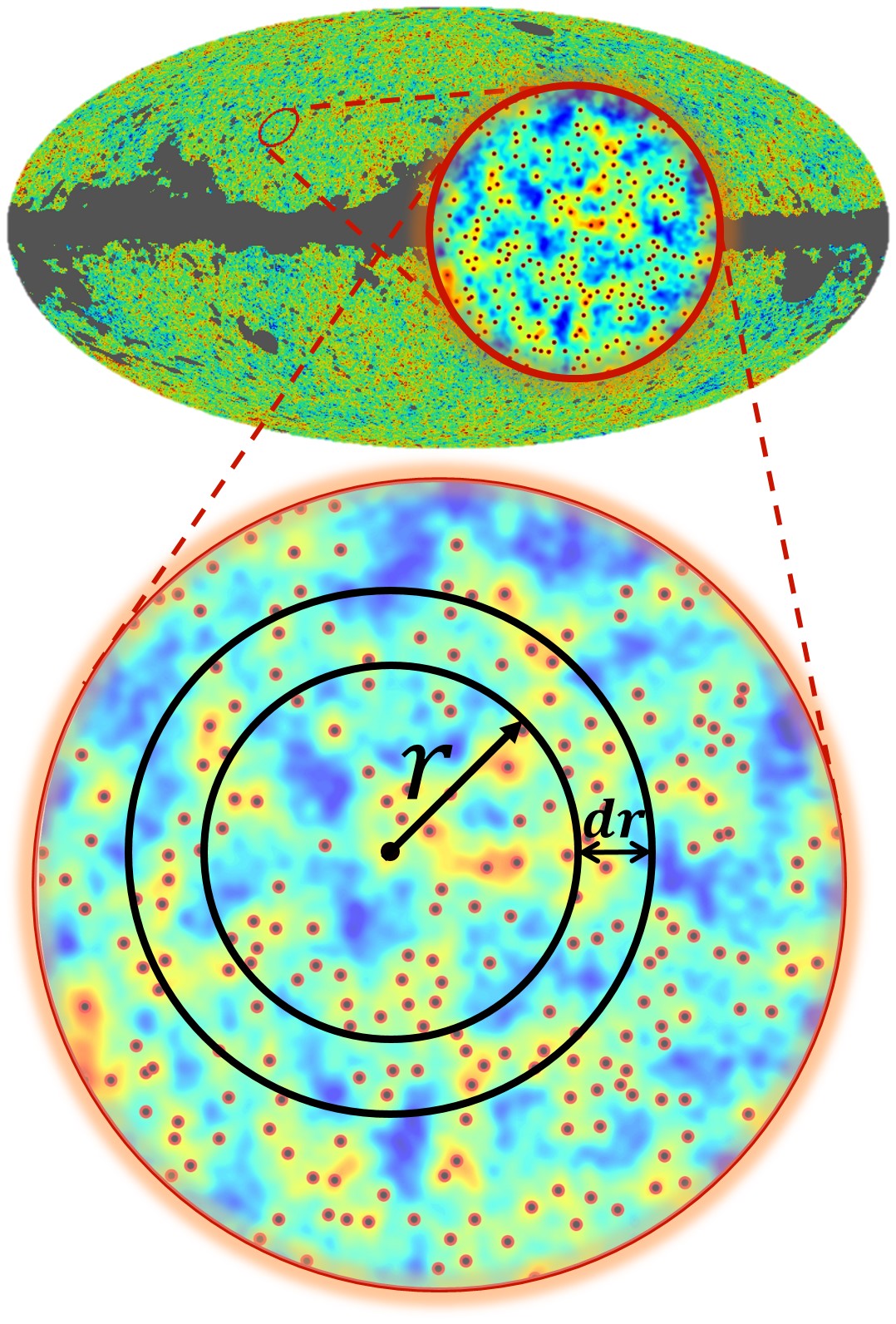
where $S_{0}\equiv\mathcal{K}^{(3)}_{111}/\sigma_{0}^{4}$ and $K_{0}\equiv\mathcal{K}^{(4)}_{1111}/\sigma_{0}^{6}$. Eq. (2.1) represents a generalized form compared to the one given by Rossi et al. (2011). Taking into account sharp clipping statistics up to $\mathcal{O}(\sigma_{0})$ results in marginal behaviour for non-Gaussianity at $\vartheta=\pm 1$. Including the various spectral indices, $\sigma_{m}$, yields more complicated theoretical formula for $n_{\rm pk}$ and $n_{\rm tr}$, and mentioned measures are more sensitive to non-Gaussianity. Perturbative expansion in the weakly non-Gaussian regime for number density of peaks and troughs have been calculated in (Pogosyan et al., 2011). In Fig. 1, we show the spatial distribution of peaks on the NILC map. In the next subsection, we will try to set up the clustering of local extrema which is systematically given by unweighted TPCF of peaks and troughs.

2.2 Unweighted Two-Point Correlation Function

The one-point statistics of some geometrical measures (number density of local extrema as well as pixels above a threshold) have been explained in previous subsection. They can explore probable exotic features and various types of non-Gaussianity (Pogosyan et al., 2011; Rossi et al., 2011; Rossi, 2013; Gay et al., 2012; Codis et al., 2013; Reischke et al., 2015). However, to do more precise evaluation, we should go beyond the one-point statistics (Hou et al., 2009; Movahed et al., 2013). In this subsection, we focus on the clustering of local extrema, which is the so-called unweighted TPCF. Semi-analytical (Heavens & Sheth, 1999; Heavens & Gupta, 2001; Matsubara, 2020) and numerical approaches (Kerscher et al., 2000) are often used to study the clustering of local extrema. The clustering of peak or trough pairs separated by distance $r=|{\bf{r}}_{1}-{\bf{r}}_{2}|$ at thresholds $\vartheta_{1}$ and $\vartheta_{2}$ is given by:

$$\langle n_{\diamond}(\textbf{r}_{1},\vartheta_{1})n_{\diamond}(\textbf{r}_{2},\vartheta_{2})\rangle=$$ (10)

$$\int{\rm d}^{6}{\mathcal{A}}_{1}{\rm d}^{6}{\mathcal{A}}_{2}\delta_{\rm D}(\textbf{r}_{1}-\textbf{r}_{\diamond 1})\delta_{\rm D}(\textbf{r}_{2}-\textbf{r}_{\diamond 2}){\mathcal{P}}({\mathcal{A}}_{1};{\mathcal{A}}_{2})$$

Taking into account the conditions for having extrema imposes some constraints on the domain of integrations (Heavens & Sheth, 1999; Heavens & Gupta, 2001). The excess probability of finding pairs using Eq. (10) becomes:

$$\Psi_{\diamond-\diamond}(r;\vartheta_{1},\vartheta_{2})=\frac{\left\langle n_{\diamond}(\textbf{r}_{1},\vartheta_{1})n_{\diamond}(\textbf{r}_{2},\vartheta_{2})\right\rangle}{n_{\diamond}(\vartheta_{1})n_{\diamond}(\vartheta_{2})}-1,$$ (11)

In our pipeline, we rely on the numerical evaluation of unweighted TPCF of local extrema in both observed and simulated maps. To this end, some robust numerical estimators for determining $\Psi_{\diamond-\diamond}(r;\vartheta_{1},\vartheta_{2})$ that are free of the boundary effect are listed below:

$$\Psi^{N}_{\diamond-\diamond}(r;\vartheta_{1},\vartheta_{2})=\left(\frac{D_{\diamond}(\textbf{r}_{1},\vartheta_{1})D_{\diamond}(\textbf{r}_{2},\vartheta_{2})}{R_{\diamond}(\textbf{r}_{1},\vartheta_{1})R_{\diamond}(\textbf{r}_{2},\vartheta_{2})}\right)\frac{N_{R}^{\diamond}(N_{R}^{\diamond}-1)}{N_{D}^{\diamond}(N_{D}^{\diamond}-1)}-1$$

$$\Psi^{H}_{\diamond-\diamond}(r;\vartheta_{1},\vartheta_{2})=\frac{R_{\diamond}(\textbf{r}_{1},\vartheta_{1})R_{\diamond}(\textbf{r}_{2},\vartheta_{2})D_{\diamond}(\textbf{r}_{1},\vartheta_{1})D_{\diamond}(\textbf{r}_{2},\vartheta_{2})}{\left[D_{\diamond}(\textbf{r}_{1},\vartheta_{1})R_{\diamond}(\textbf{r}_{2},\vartheta_{2})\right]^{2}}-1$$

$$\Psi^{LS}_{\diamond-\diamond}(r;\vartheta_{1},\vartheta_{2})=\left(\frac{D_{\diamond}(\textbf{r}_{1},\vartheta_{1})D_{\diamond}(\textbf{r}_{2},\vartheta_{2})}{R_{\diamond}(\textbf{r}_{1},\vartheta_{1})R_{\diamond}(\textbf{r}_{2},\vartheta_{2})}\right)\frac{N_{R}^{\diamond}(N_{R}^{\diamond}-1)}{N_{D}^{\diamond}(N_{D}^{\diamond}-1)}-\left(\frac{D_{\diamond}(\textbf{r}_{1},\vartheta_{1})R_{\diamond}(\textbf{r}_{2},\vartheta_{2})}{R_{\diamond}(\textbf{r}_{1},\vartheta_{1})R_{\diamond}(\textbf{r}_{2},\vartheta_{2})}\right)\frac{N_{R}^{\diamond}(N_{R}^{\diamond}-1)}{N_{D}^{\diamond}N_{R}^{\diamond}}+1$$

$\Psi^{N}$ is called the ’natural estimator’ (Landy & Szalay, 1993). $\Psi^{H}$ is proposed by Hamilton (1993) while $\Psi^{LS}$ introduced by Landy & Szalay (1993) has a nearly Poisson variance. In the above equation, $D_{\diamond}(\textbf{r}_{1},\vartheta_{1})D_{\diamond}(\textbf{r}_{2},\vartheta_{2})$ and $R_{\diamond}(\textbf{r}_{1},\vartheta_{1})R_{\diamond}(\textbf{r}_{2},\vartheta_{2})$ represent the number of peak or trough pairs in the data and random catalogs, respectively, and $D_{\diamond}(\textbf{r}_{1},\vartheta_{1})R_{\diamond}(\textbf{r}_{2},\vartheta_{2})$ corresponds to cross-pairs. In the above equations, $N_{D}^{\diamond}$ and $N_{R}^{\diamond}$ are respectively the total number of local extrema in the data and random catalogs. The lower part of Fig. 1, indicates the peak pairs separated by $r$ in a magnified patch.

2.3 General definition of bias factor

The general statistical expression for the relation between unweighted TPCF as the excess probability of finding a typical feature and the weighted TPCF which is known as auto-correlation function at the first-order approximation, reveals a linear and scale-independent bias factor. For a Gaussian random field, the excess probability of finding the sharp clipping pairs is statistically magnified by the fluctuation of random field for long separation distance (angle) at high threshold, $\vartheta\gg 1$. In this regime, we have $\Psi_{\rm pix-pix}(\theta;\vartheta)\sim e^{\mathcal{B}^{2}_{\rm pix}(\vartheta)C_{TT}(\theta)}-1$ with $\mathcal{B}_{\rm pix}(\vartheta)\sim\vartheta$ (Kaiser, 1984; Taqqu, 1977; Politzer & Wise, 1984; Jensen & Szalay, 1986; Bardeen et al., 1986; Szalay, 1988a, b) (for extensive discussion see (Martinez & Saar, 2001; Desjacques et al., 2018, and references therein)).

Now, we turn to the modulation of local maxima number density at threshold $\vartheta$ in the CMB map by the temperature fluctuations at the last scattering surface. In other words, we look for the relation between the unweighted TPCF of peaks and weighted TPCF of temperature fluctuations. The general form of the bias factor enables us to estimate the unweighted TPCF of typical feature by using the weighted TPCF. Generally, we expect that the number density of peaks is enhanced where the temperature fluctuations are high. For the CMB map, we define the peaks number density contrast as: $\delta_{\rm pk}\equiv\frac{n_{\rm pk}-\langle n_{\rm pk}\rangle}{\langle n_{\rm pk}\rangle}$. To determine the scale-independent bias factor averaged on all peak curvature values, we are interested in examining a relation such as $\delta_{\rm pk}=\mathcal{B}_{\rm pk}(\vartheta)\delta_{T}$. Following Kaiser (1984) for sharp clipping statistics, we exploit a systematic relation between unweighted TPCF of local extrema, $\Psi_{\diamond-\diamond}(\theta;\vartheta_{1},\vartheta_{2})$, and weighted TPCF of temperature fluctuations, $C_{TT}(\theta)$, for separation angle, $\theta$, in analogy with $\Psi_{\diamond-\diamond}(\theta;\vartheta)={\mathcal{B}}^{2}_{\diamond}(\vartheta)C_{TT}(\theta)$, when we ignore the scale-dependent part. The relation mentioned is satisfied for large separation angles. For very high threshold values, the pixel above threshold can delineate the peak better than a small threshold and consequently we obtain $\mathcal{B}_{\rm pk}(\vartheta)\sim\mathcal{B}_{\rm pix}(\vartheta)$ for large enough separation angles in a Gaussian field (Martinez & Saar, 2001). To examine the scale-dependent part of the bias for peak statistics, we rely on a more general model for bias in the Fourier space as: $\mathcal{B}_{\rm pk}(k,\vartheta)=\mathcal{B}_{\rm pk}(\vartheta)+\mathcal{B}_{k}^{\rm pk}(\vartheta)k^{2}$. Here $k$ represents the wavelength of the typical mode. It turns out that for either $\vartheta\gg 1$ or large scales, the value of scale-dependent part of bias is $\mathcal{B}_{k}^{\rm pk}(\vartheta)\to 0$ (Desjacques et al., 2010; Desjacques et al., 2018). We define $\mathcal{B}^{2}_{\diamond}(\theta,\vartheta)\equiv\Psi_{\diamond-\diamond}(\theta;\vartheta)/C_{TT}(\theta)$ for proper range of $\theta$. Subsequently, any features existing in $\mathcal{B}^{2}_{\diamond}(\theta,\vartheta)$ versus $\theta$ for a typical value of $\vartheta$ represent the contribution of the scale in this type of bias factor. We will assess the behaviour of such a bias factor and accordingly the consistency of Planck maps and associated state-of-the-art simulations.

Figure 2: Colour online: Upper panel corresponds to the cumulative number density of peaks above a threshold, $n_{\rm pk}(\vartheta)$, for various observed CMB data (solid lines) compared to associated end-to-end simulations (dashed line) at the top part and the corresponding differences, $\Delta n_{\rm pk}(\vartheta)$, at the bottom part of this panel, respectively. The lower panel indicates the cumulative number density of troughs below a threshold, $n_{\rm tr}(\vartheta)$, at the top and the differences, $\Delta n_{\rm tr}(\vartheta)$, at the bottom, respectively. The difference plots are given to clarify how tiny the deviation is. The solid lines with different colours in mentioned plots show the residues of different component separations for observation and the shaded region corresponds to the $2\sigma$ confidence interval determined by the ensemble average on fiducial Gaussian CMB simulations. We considered $N_{\rm{side}}=2048$.

3 Data description and simulation

The Planck sky observational data sets contain full-sky maps at nine frequency channels for temperature intensity. The polarization maps are available only for 30-353 GHz frequency range. Throughout this paper, we only focus on the temperature field. The mentioned data sets are processed by the $Planck$ team, resulting in different component separation algorithms, namely Commander-Ruler (CR), NILC, SEVEM and SMICA (Planck Collaboration et al., 2020c); these are publicly available and are provided in the HEALPIX format (Gorski et al., 2005). Such component separation algorithms allow us to achieve the largest possible sky area coverage. In addition, these procedures can remove galactic emission and reconstruct the diffuse emission from our galaxy (see Dickinson (2016) for a comprehensive description of the CMB foreground). The latest proper mask and the corresponding fraction of unmasked pixels used for the CMB data are specified by UT78 and $f_{\rm{sky}}=77.6\%$, respectively (Planck Collaboration et al., 2016a, c). To realize reliable statistical inferences about the number density of the local extrema and associated clustering, we also need fiducial simulations as the reference sets and for debiasing in our statistical analysis. To this end, we use 500 realizations of the end-to-end simulations (Planck Collaboration et al., 2020a, b), where they are publicly available on Planck Legacy Archive. The end-to-end fiducial CMB power spectrum is based on the $\Lambda$CDM model with the best-fitting Planck parameters (Planck Collaboration et al., 2020d). To interpret our results, the fiducial maps would be the Gaussian-based expectation. To avoid obtaining spurious results, we will compare the results in the context of local extrema analysis of each component separation outcomes with corresponding simulations.

4 Implementation on real data and synthetic data sets

In this section, we apply our statistical measures based on critical sets explained in Section 2 on the Planck CMB maps and corresponding end-to-end simulated data sets.

Figure 3: The number density of peaks (upper panel) and troughs (middle panel) as a function of threshold for Planck data sets and corresponding Gaussian simulations. The number density of pixel at the threshold is illustrated in the lower panel. In the lower part of each panel, we have computed the difference of number density with corresponding simulated map. The shaded region corresponds to the $2\sigma$ optimal variance error determined by fiducial Gaussian CMB map. The solid lines with different colours in the mentioned plots show the residues of different component separations for observation and the shaded region corresponds to the $2\sigma$ confidence interval determined by the ensemble average on fiducial Gaussian CMB maps. We considered $N_{\rm{side}}=2048$.

Figure 4: The unweighted TPCF of peaks for the CMB observed maps considering $\vartheta\geq[-2.0-1.5]$. The simulation in this plot corresponds to the end-to-end $\Lambda$CDM Gaussian CMB map. The solid lines show the results for the different component separations, while the dashed lines show ensemble average based on end-to-end simulations and the shaded region corresponds to the $2\sigma$ level of confidence.We considered $N_{\rm{side}}=2048$.

4.1 Local extrema statistics of CMB map

Critical regions among of excursion sets are efficient measures to recognize exotic features in the CMB maps. To start, we turn to one-point statistics of sharp clipping and local extrema.The latter is more complicate due to the conditions required for extrema, while the former is more slightly less sensitive to searching for probable exotic features.

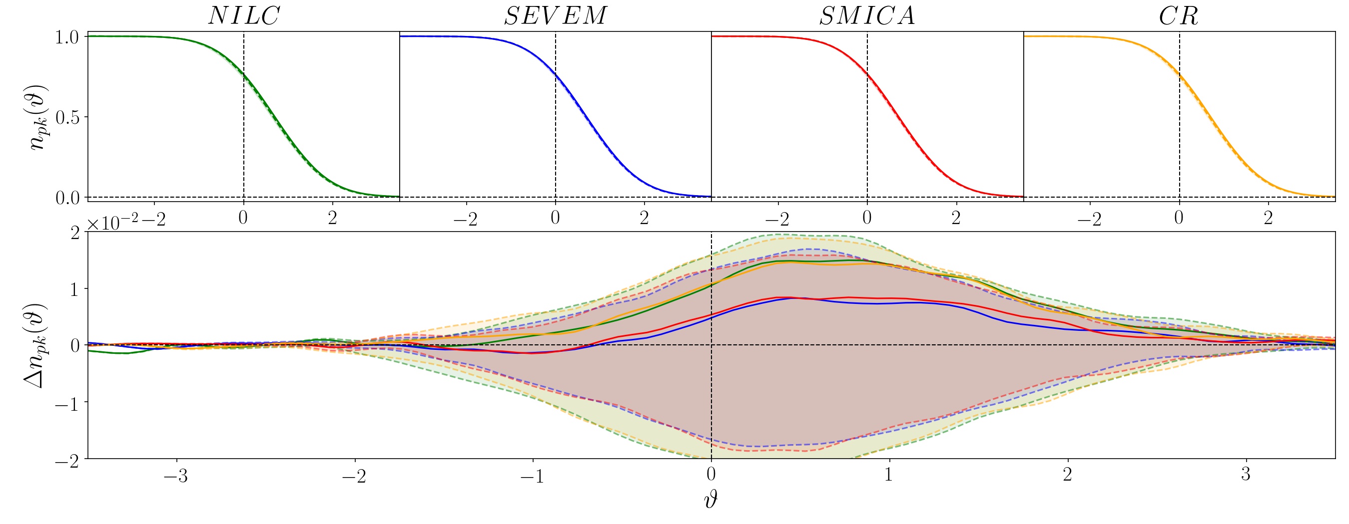
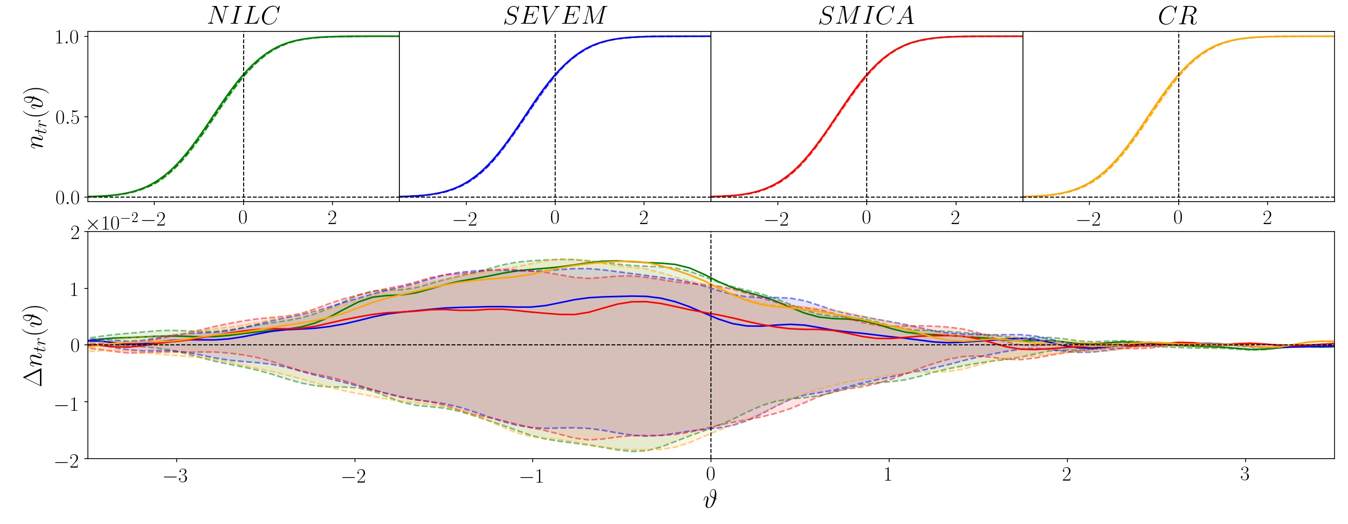
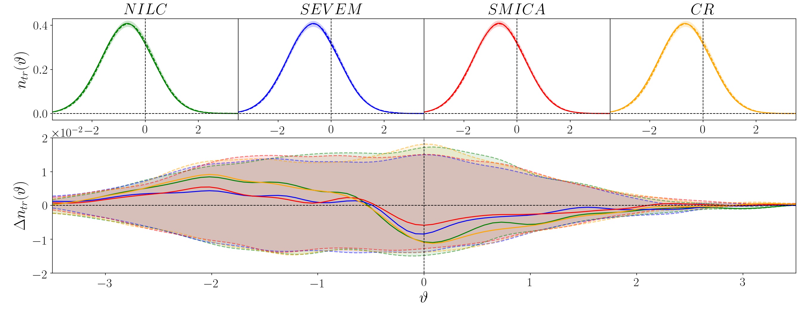
Fig. 2 illustrates the normalized cumulative number density of local maxima for different types of observed data, while the lower panel illustrates the cumulative number density of troughs below the threshold. To recognize the deviation between each component separation product and associated end-to-end simulation, we compute $\Delta n_{\rm pk}$ and $\Delta n_{\rm tr}$ which are depicted in the lower part of upper and lower panels, respectively. In mentioned plot, the solid lines correspond to the results for the observed map, while the dashed line are for associated end-to-end simulations. The shaded region represents the $2\sigma$ level of confidence. According to the $n_{\rm tr}$ statistics, our results show that the NILC and CR have small deviations from corresponding simulations around the $\sim\vartheta\in[-2-0]$, while the cumulative peak number density of all observed maps are consistent with each other. Our results also confirm that the values of the cumulative number density of peaks and troughs for all observed maps are higher than those values computed for the wide range of thresholds.

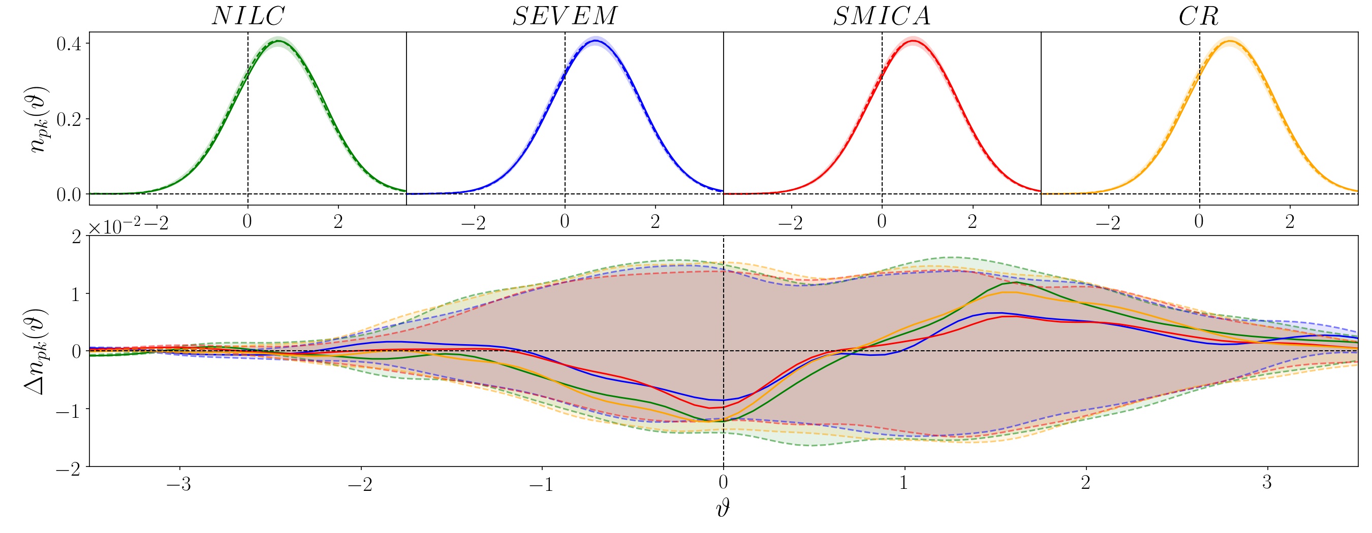
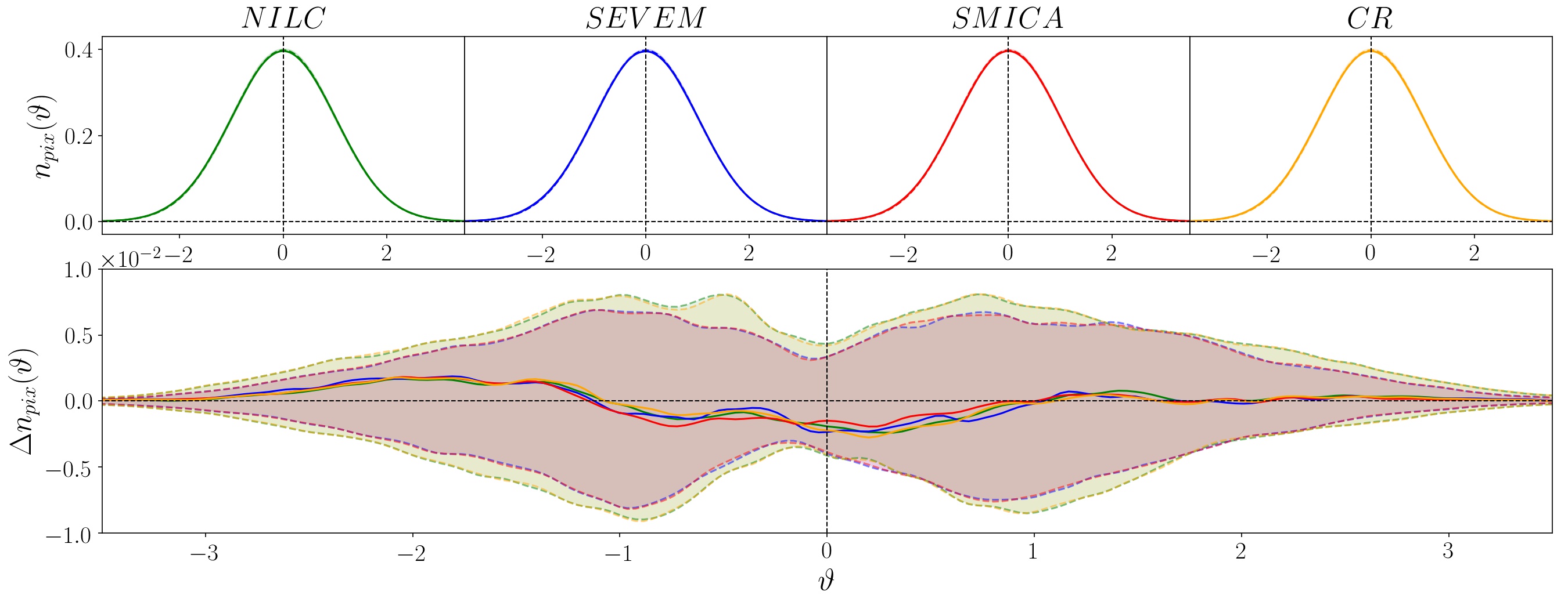
Fig. 3 depicts the number density of local maxima (upper panel), local minima (middle panel) and pixel (lower panel) at the threshold. All observations display very tiny deviation at mean threshold ($\vartheta\approx 0$). We should point out that, according to the local extrema number density at the mean threshold, all component separations data sets are located below the corresponding values computed for simulations. It turns out that the sharp clipping statistics is less sensitive to non-Gaussianity and represents more consistency with simulated maps (lower panel of Fig. 3). Another interesting result is that, there is no significant difference between $n_{\rm pk}(\vartheta)$ and $n_{\rm tr}(-\vartheta)$ for all of the CMB maps, as expected for a Gaussian field.

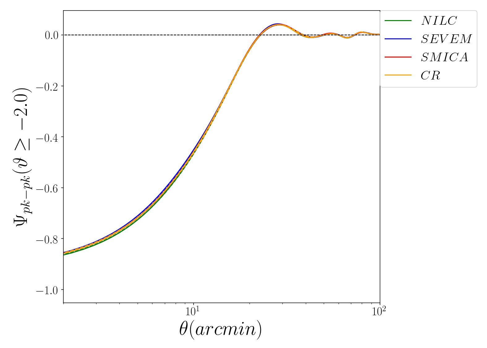
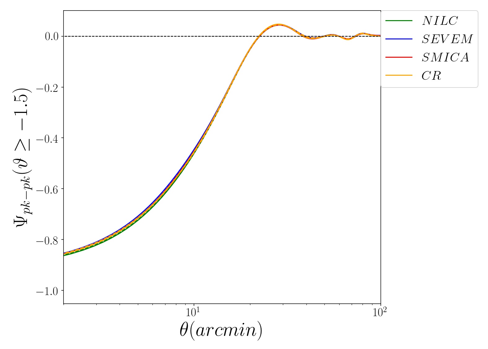
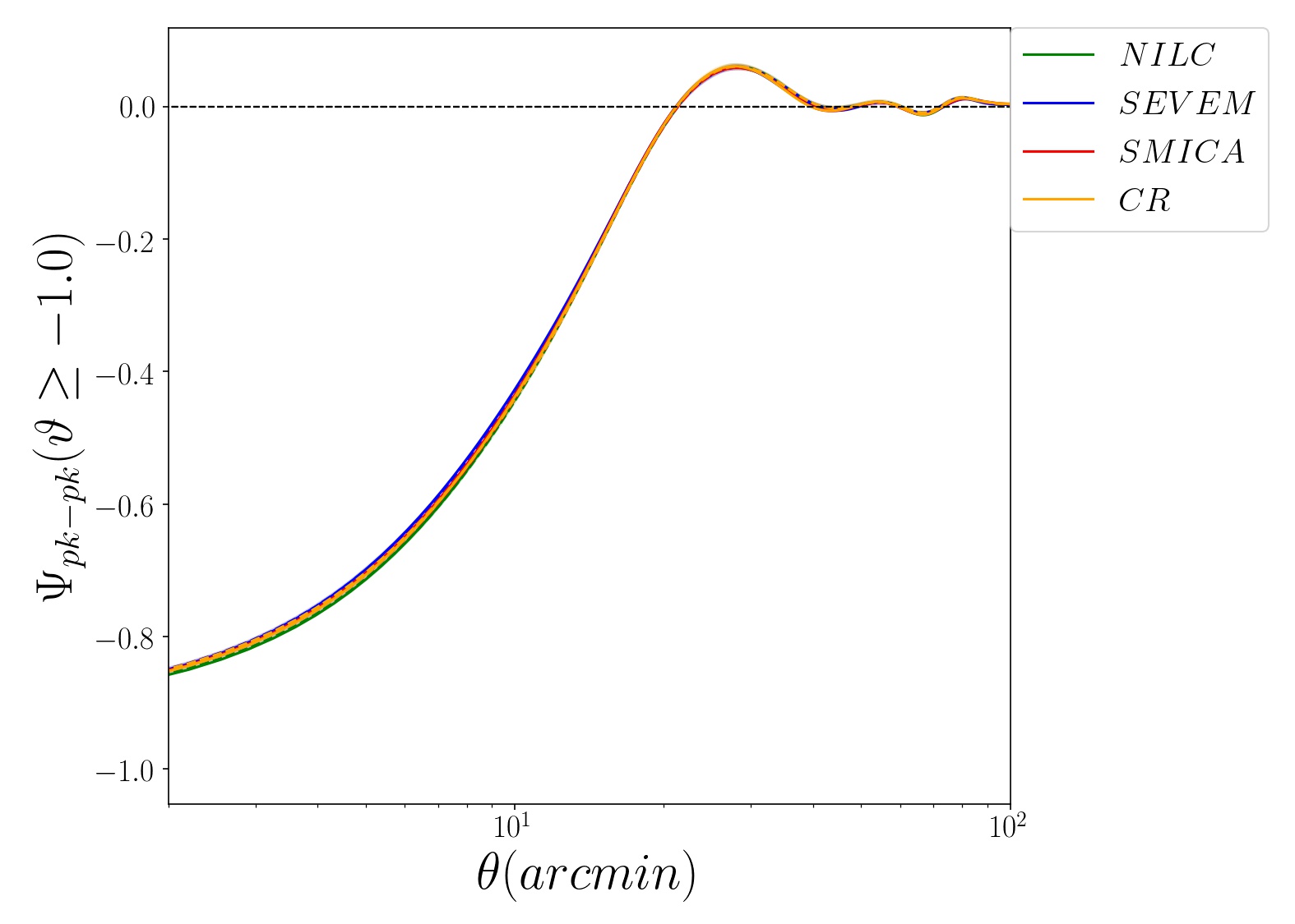
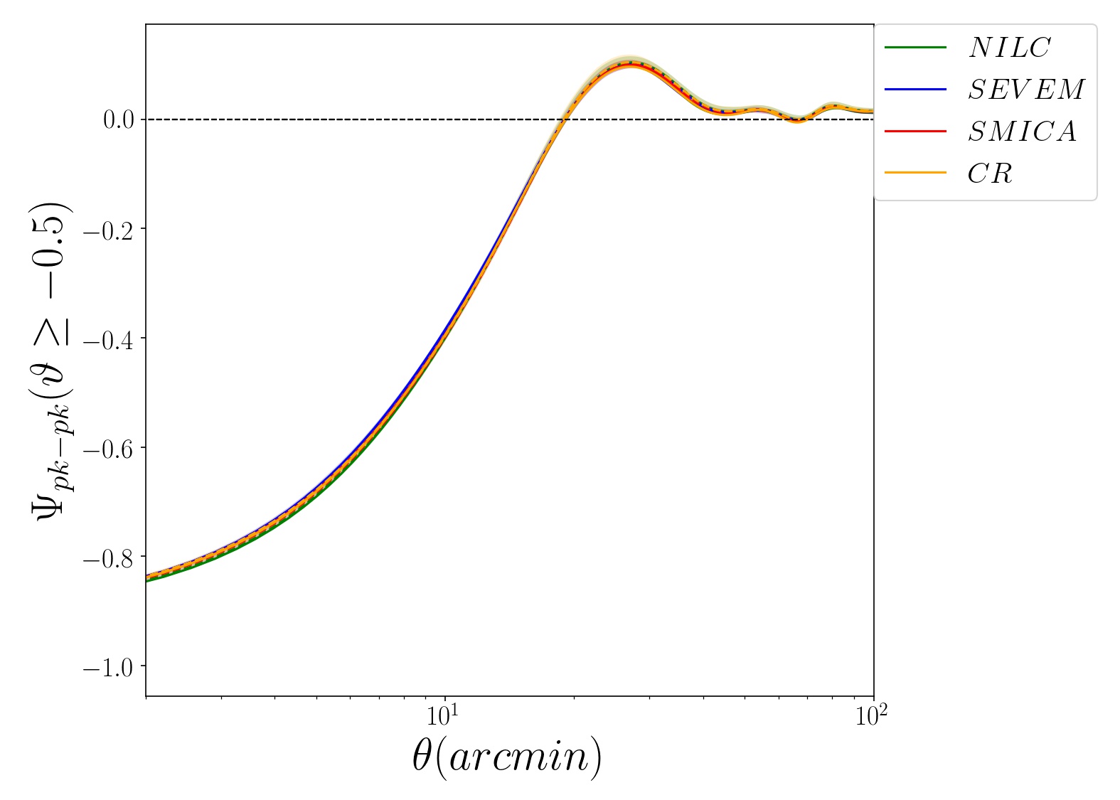
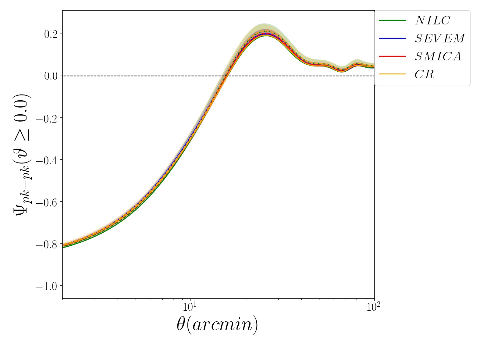
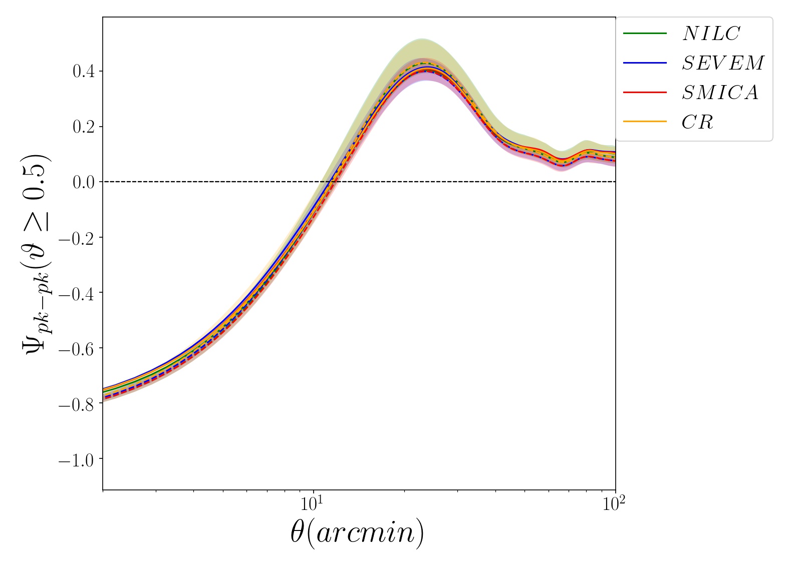
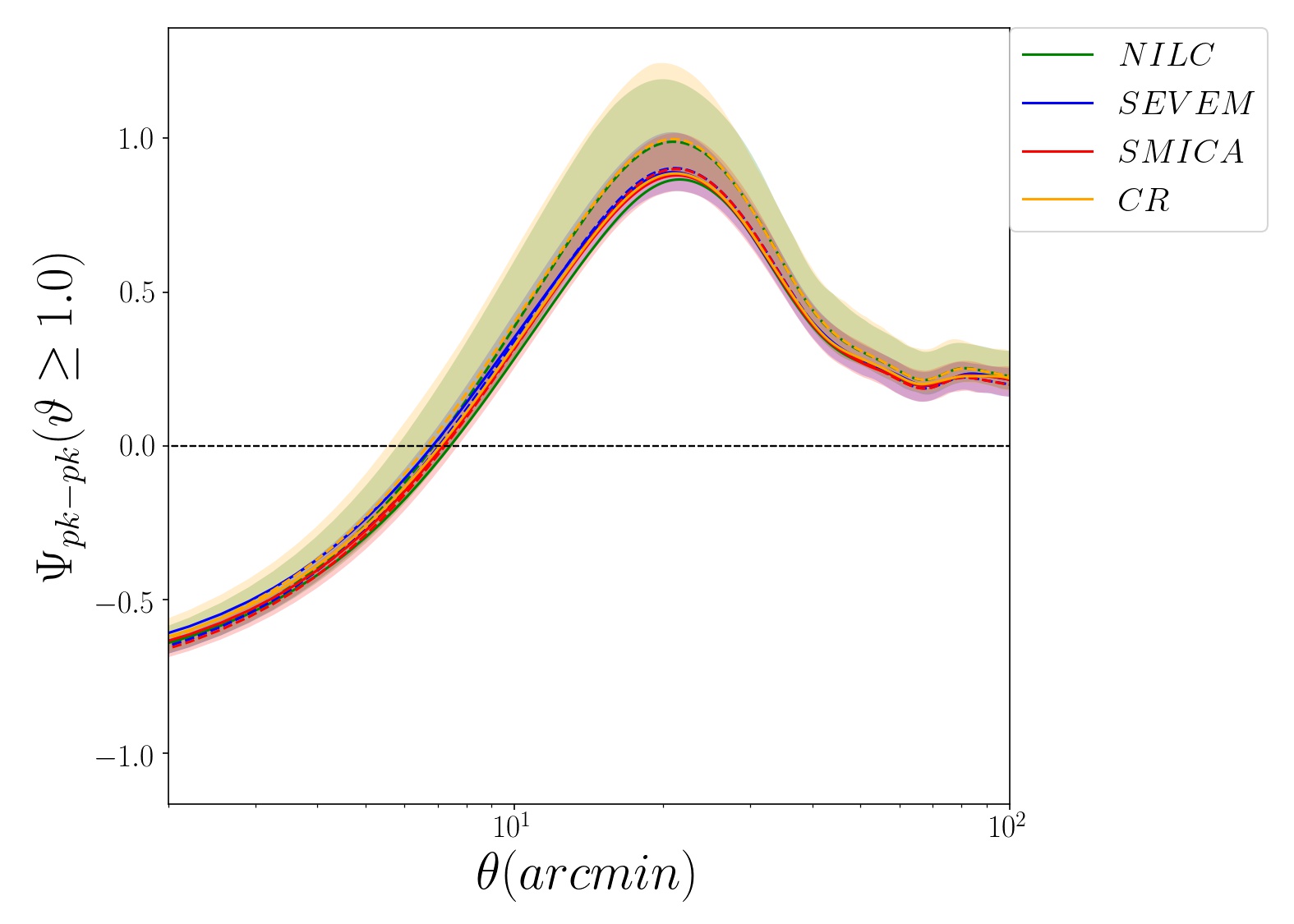
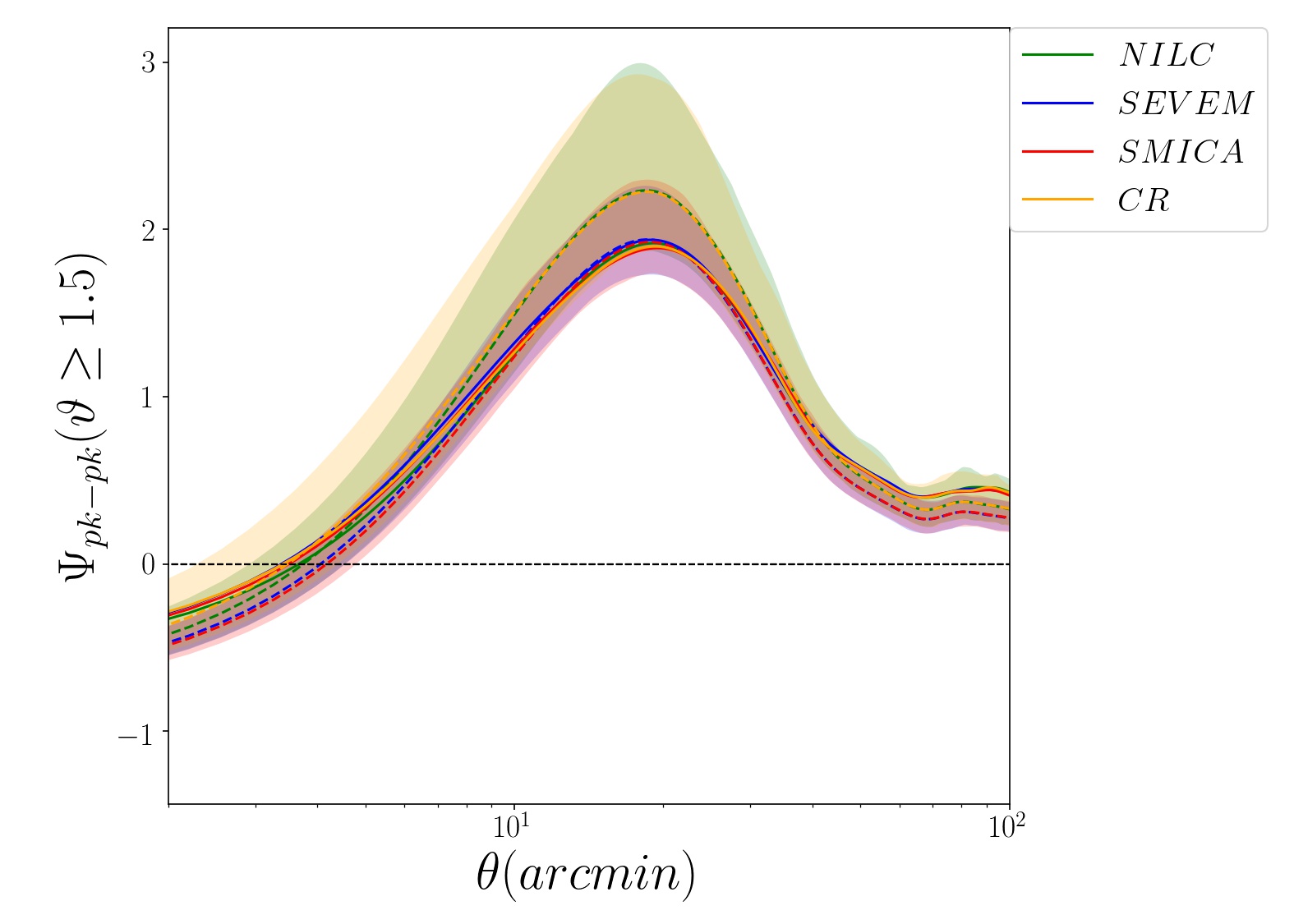
Going beyond the one-point statistics of critical sets provides a proper opportunity for examining exotic features and enables us to reduce the spurious and artificial effects due to undesired non-cosmological sources. Therefore, we use unweighted TPCF of local extrema. To this end, we check all the estimators introduced by Eqs. (2.2), (2.2) and (2.2). Our analysis demonstrates that all results are consistent with each other. Consequently, for the rest of this paper, we will show what we have obtained by the Hamilton estimator (Eq. (2.2)). We find all the peaks and troughs above thresholds in the interval that corresponds to $-3\leq\vartheta\leq 3$ with step size $0.5$ in each full sky simulated map and then apply unweighted TPCF estimator to compute $\Psi_{\diamond-\diamond}(\theta;\vartheta)$ for both observed and simulated maps. The final results for simulation are given by doing ensemble average over 500 realizations. Such results play the role of numerical results for the Gaussian map. The unweighted TPCF of peaks as a function of separation angle is shown in Fig. 4 for Planck data above a given threshold for different component separation algorithms. The solid lines are associated with Planck CMB maps, while the dashed lines represent the unweighted TPCF for end-to-end simulations. The clustering of local maxima demonstrates that all observed map are consistent with the Gaussian hypothesis. However, there is a lack of peak clustering for high enough threshold around $10^{\prime}\lesssim\theta\lesssim 30^{\prime}$ compared to the Planck fiducial $\Lambda$CDM model. For $\vartheta\geq 1.0$, small difference between various component separations is also seen.

We also assess the unweighted TPCF of peaks for $\delta_{T}<-\vartheta\sigma_{0}$ and for $\delta_{T}>+\vartheta\sigma_{0}$. For an ideal Gaussian random field, we expect to have $\Psi_{\diamond-\diamond}(\delta_{T}<-\vartheta\sigma_{0})=\Psi_{\diamond-\diamond}(\delta_{T}>+\vartheta\sigma_{0})$ due to symmetry between peaks and troughs. Our results confirm that observed CMB data are consistent with this expectation. While clustering of the pixels above and below a threshold for $WMAP$ data done by Rossi et al. (2009), showed different results for large separation angle . This achievement clarifies that peak-peak statistics rather than pixel-pixel analysis is more robust in the presence of probable un-resolve noises and other unknown effects. Also, the updated observed maps reveals more consistency with expected Gaussian properties, if we utilize the clustering of local extrema rather than pixels clustering.

Figure 5: The value of angular separation at which the unweighted TPCF of peaks reaches its maximum value ($\theta_{\rm bump}$) as a function of threshold is indicated in the upper panel. The lower panel shows the value of the unweighted TPCF of peaks around Doppler peak, $\theta\approx 75$ arcmin as a function of threshold. The solid lines show the results of different component separations for observation, the dashed lines correspond to the end-to-end simulations prepared for each observed map, and the shaded region corresponds to the $2\sigma$ region to see deviation from fiducial Gaussian CMB maps. We considered $N_{\rm{side}}=2048$.

Figure 6: The scale-independent bias factor for peaks above a threshold for CMB simulated data and SMICA maps is illustrated in the upper panel. The dashed line shows the results for pixels above a threshold given by theory for a Gaussian field while the filled circle symbol with a line is for peaks above threshold for a simulated CMB map. The symbols indicate the results for observation. The lower panel corresponds to the evaluation of scale-dependent bias for peak statistics above a threshold. The dashed lines show results for the end-to-end simulated map corresponding to SMICA while the solid lines show for SMICA. The shaded region corresponds to the $2\sigma$ region to see deviation from the fiducial Gaussian CMB maps where $N_{\rm{side}}=2048$.

Table 1: Probabilities of obtaining values of the $\chi^{2}$ statistics represented by $P(\chi^{2}>\chi^{2}_{\diamond-\diamond}(\vartheta))$, $P(\chi^{2}>\chi^{2}_{\rm pix})$, $P(\chi^{2}>\chi^{2}_{\rm pk})$ and $P(\chi^{2}>\chi^{2}_{\rm tr})$ for the Planck fiducial $\Lambda$CDM Gaussian model at least as large as the observed values for various observed maps. Here we consider $N_{\rm side}=2048$.

Map/Measure	$n_{pix}$	$n_{pk}$	$n_{tr}$	$\Psi_{tr-tr}(\vartheta\leq 0.0)$	$\Psi_{tr-tr}(\vartheta\leq-1.0)$	$\Psi_{pk-pk}(\vartheta\geq 0.0)$	$\Psi_{pk-pk}(\vartheta\geq 1.0)$
NILC	0.42	0.88	0.57	0.13	0.74	0.22	0.70
SEVEM	0.88	0.54	0.72	0.36	0.86	0.46	0.79
SMICA	0.60	0.22	0.64	0.62	0.26	0.21	0.40
CR	0.26	0.12	0.72	0.59	0.62	0.37	0.54

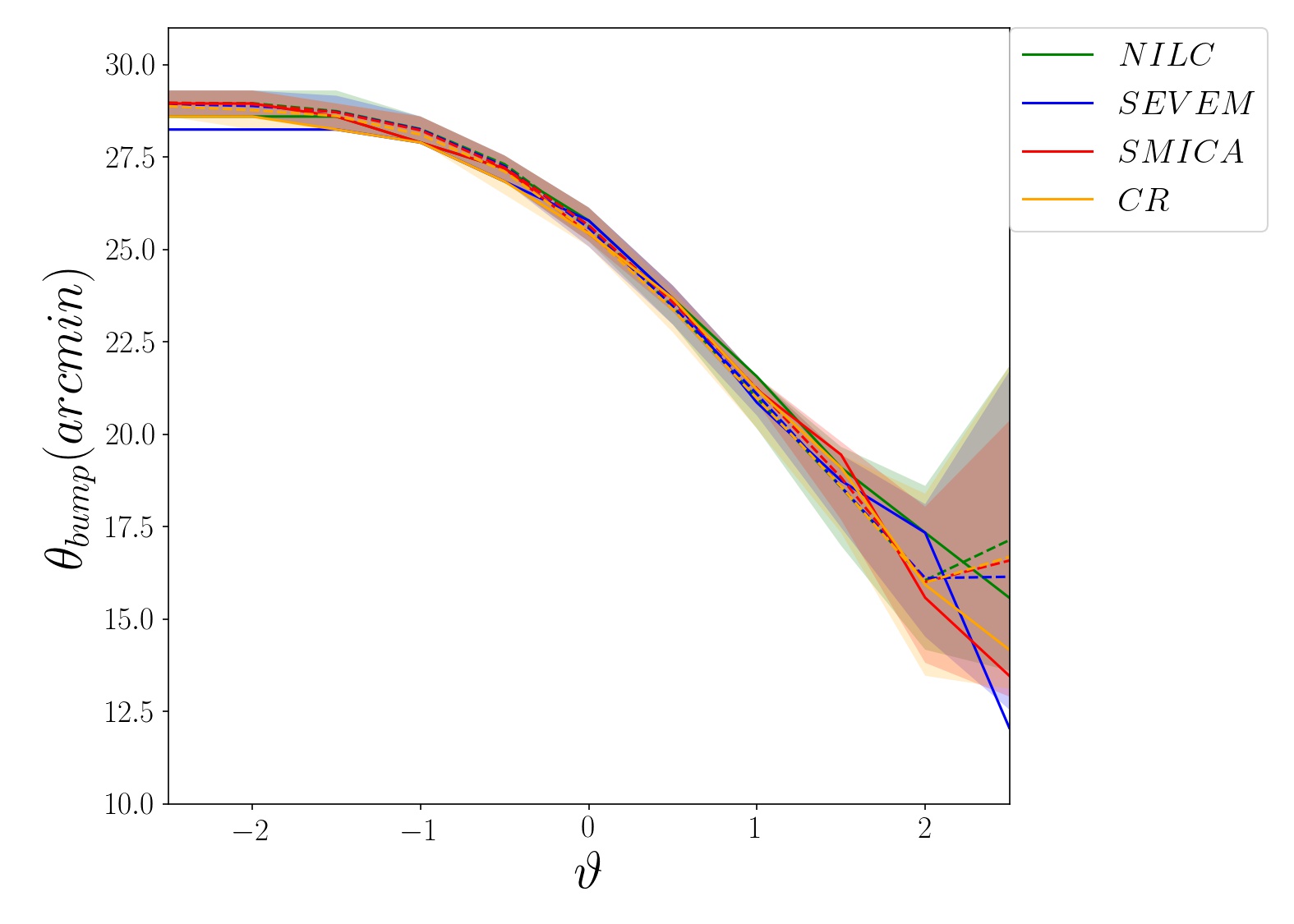
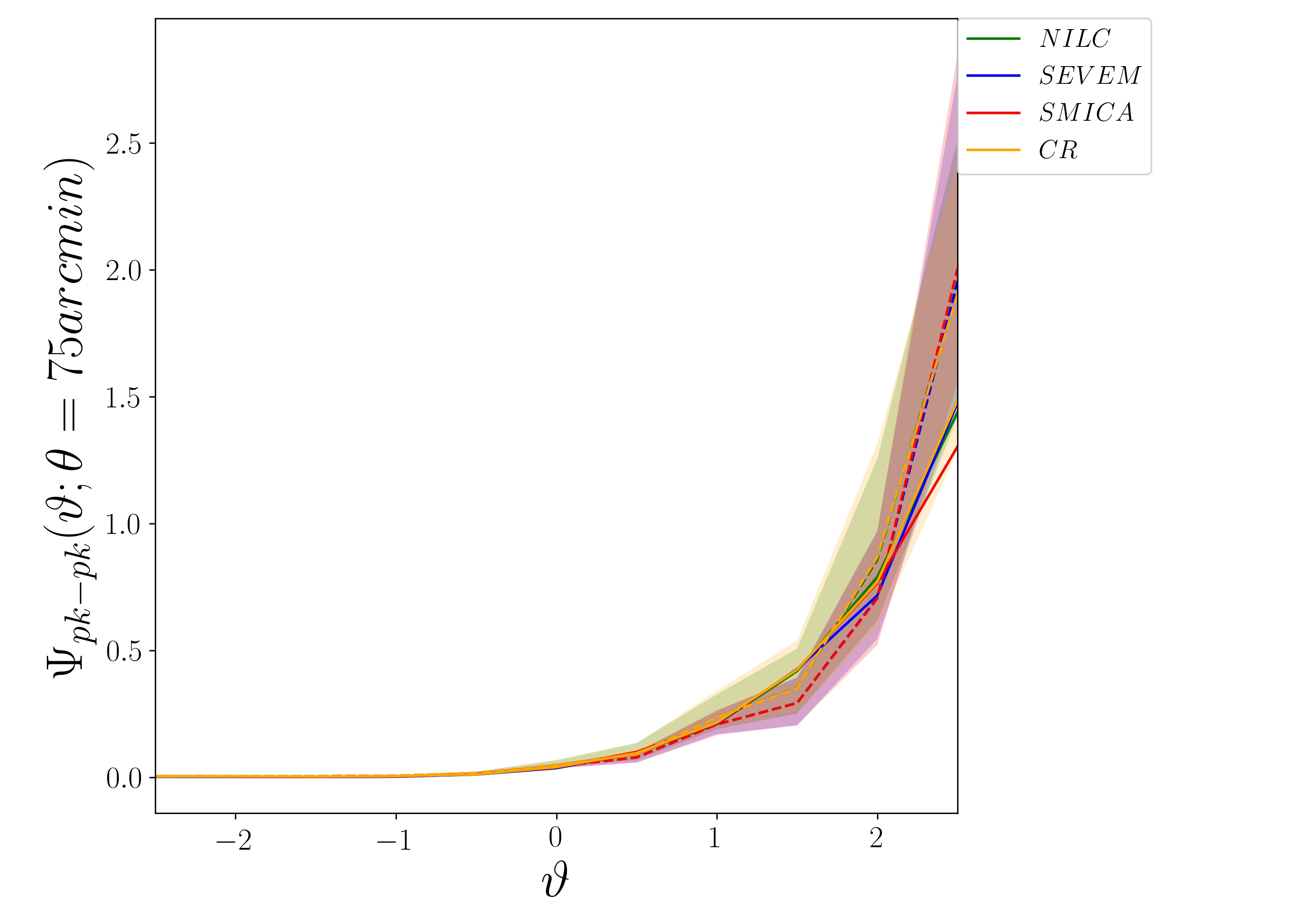
The position of so-called bump for unweighted TPCF of peaks above a given threshold versus $\vartheta$ is indicated in the upper panel of Fig. 5. The lower panel corresponds to the value of unweighted TPCF of peaks around Doppler peak, $\theta\sim 75$ arcmin, as a function of threshold. In this plot, we depict the results for observed maps by the solid lines and dashed lines are refereed to the associated end-to-end simulations drawn in the same colours. According to the semi-analytical approach (see Heavens & Sheth (1999)), by increasing the threshold, the unweighted TPCF of peaks in a Gaussian CMB map reaches its maximum value for lower separation angle. Such behaviour can be justified by means of the distribution of local maxima at higher threshold which is more distinguishable from random catalog. Applying the different beam size can also wash out the peaks and suppressing the bump in $\Psi$ for all thresholds (Heavens & Sheth, 1999). The value of $\theta_{\rm bump}$ for observed maps is almost less than synthetic data for high thresholds. The value of extrema clustering around the Doppler peak for higher threshold in the Planck observed data is less than the corresponding value in the simulated maps. However, taking into account statistical errors, mentioned deficiency is not statistically significant.

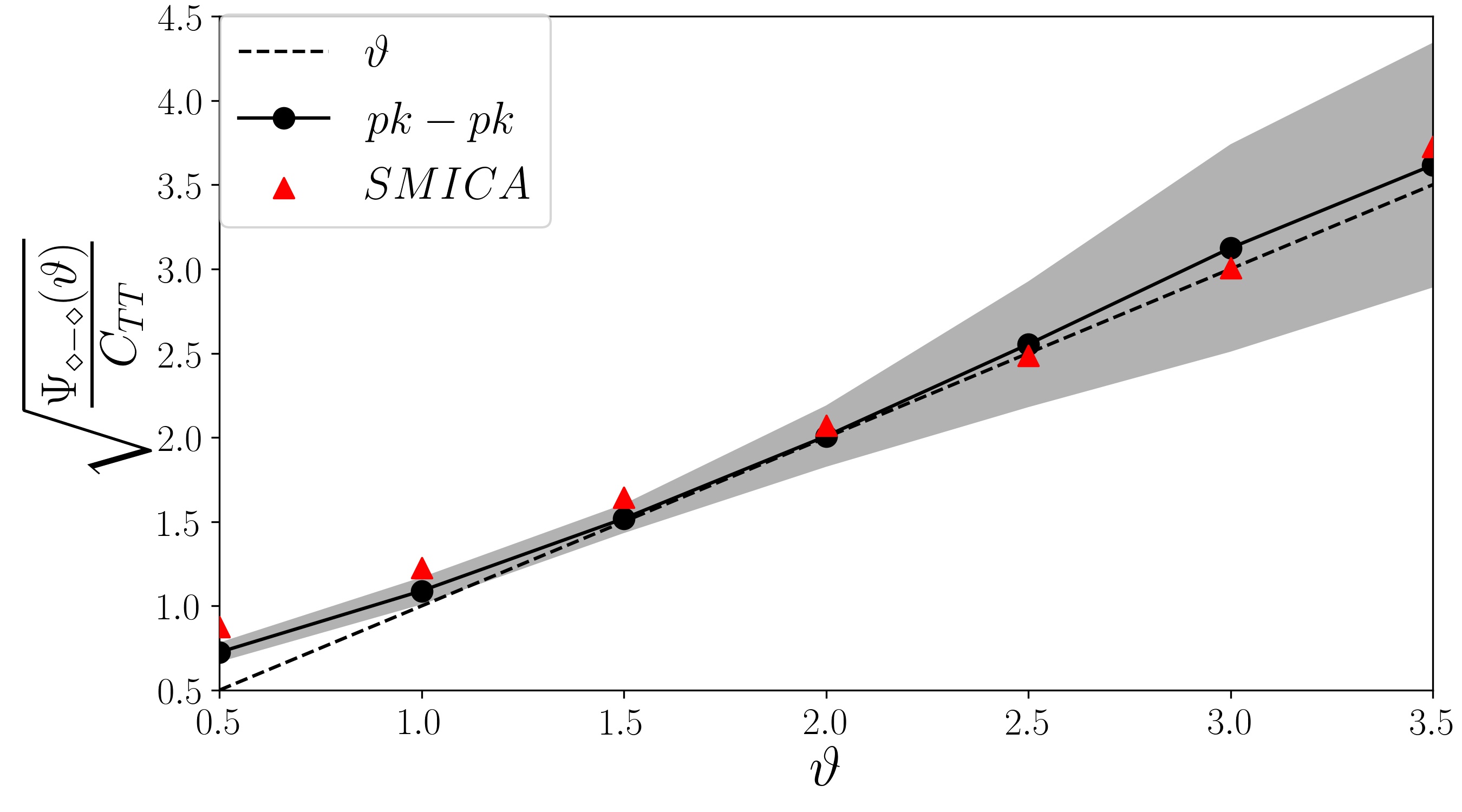
According to the researches done by Takada et al. (2000); Takada & Futamase (2001), the bump and main trough around the Doppler peak in the unweighted TPCF of peaks are more sensitive to the effect of gravitational lensing on the CMB photons which are randomly deflected by foreground ranging from large scale structures to cosmic strings networks. In other words, redistribution of peak in the CMB map from intrinsic separation and distribution by weak lensing phenomenon have unique signature on the $\Psi_{\diamond-\diamond}$. The contribution of weak lensing on the $\Psi_{\diamond-\diamond}$ leads to mitigate the depth of Doppler peak and even suppressing the maximum value of $\Psi$ as a function of separation angle (Takada & Futamase, 2001). To put proper constraint on the amplitude of the mass fluctuations, we need more deep troughs around $\theta\approx 70^{\prime}-75^{\prime}$, consequently, according to Fig. 4, we should compute $\Psi_{\diamond-\diamond}$ for mean threshold due to more compatibility between different separation components of CMB achieved for higher thresholds around Doppler peak.

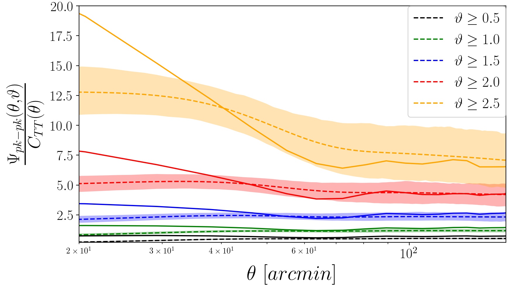
The upper panel of Fig. 6 indicates the scale-independent bias factor for peaks above a threshold for SMICA map and corresponding Gaussian simulated data sets. Here, we average on the ratio of $\Psi_{\rm pk-pk}/C_{TT}$ for large enough separation angle for each threshold denoted by symbols. For a Gaussian stochastic field, we expect to have ${\mathcal{B}}_{\rm pix}(\vartheta)\sim\vartheta$, for high threshold (Kaiser, 1984; Taqqu, 1977; Politzer & Wise, 1984; Jensen & Szalay, 1986; Bardeen et al., 1986; Szalay, 1988a, a). Semi-analytical investigation at very high threshold clarifies that, peak and pixel statistics become identical and our results are compatible with Gaussianity. Such result have been obtained for other type of observed maps and we avoid to show them for convenience.

To examine the contribution of angular scale in the bias, we compute ${\mathcal{B}}_{pk}(\theta,\vartheta)$ as a function of $\theta$ for some typical thresholds. The lower panel of Fig. 6 illustrates the unweighted TPCF of peaks to the temperature fluctuations correlation function ratio, versus scale for various thresholds. In this panel the dashed lines correspond to the Gaussian CMB simulated map extracted from end-to-end pipeline associated with SMICA, while solid line is devoted to SMICA map. The presence of some features particularly in the angular scale interval, $20$ arcmin $\lesssim\theta\lesssim 80$ arcmin, confirms that for small scale, the footprint of scale essentially appears in the bias factor, while for large enough separation angle, such features are diminished. In the latter regime and for $\vartheta\gg 1$, we expect to have a plateau for $\mathcal{B}^{2}$ and its value is proportional to $\vartheta^{2}$. It is worth mentioning that, the results for $Planck$ data sets are compatible with that expected for Gaussian field, while for small scales, we have some deviations from the results given for simulated map. By increasing the threshold, the consistency between $Planck$ data and simulations increases. Other component separations reveal almost similar results.

Figure 7: The violin plot for amplitude of the dipole power spectrum of local $\chi^{2}$ (Eqs. (4.3) and (4.3)) considering the $n_{\rm pk}$, $n_{\rm tr}$ marginalized on all available thresholds, $\Psi_{\rm pk-pk}$ and $\Psi_{\rm tr-tr}$ integrated out on some separation angles. We took threshold ranges, $\vartheta\geq 0.0$ and $\vartheta\geq 1.0$ for clustering of peaks, while, for the unweighted-TPCF of troughs, the following threshold ranges have been taken into account, $\vartheta\leq-1.0$, $\vartheta\leq 0.0$. The star symbol in each panel indicates the value computed for the observed map.

4.2 Testing Gaussian Hypothesis

Non-Gaussianity in the CMB data can be produced by late phenomena such as gravitational lensing, the Sunyaev-Zel’dovich effect, contaminations from foreground and residual point sources. Primordial non-Gaussianity can be generated by a sequence of phase transitions and deviation from uncorrelated initial fluctuations during the inflationary epoch (Komatsu, 2002; Lewis & Challinor, 2006; Planck Collaboration et al., 2014b, 2016d, 2020f).

To probe the hypothesis of Gaussianity, many statistical approaches have been proposed (Heavens & Sheth, 1999; Tojeiro et al., 2006; Rossi et al., 2009; Rossi et al., 2011; Planck Collaboration et al., 2014b, 2016d; Novaes et al., 2016; Cole & Shiu, 2018; Buchert et al., 2017; Planck Collaboration et al., 2014a, 2016c, 2020e, and references therein). The Planck team also carried out the peak statistics in addition to the other methods to asses non-Gaussianity in $Planck$ maps (Planck Collaboration et al., 2016c, 2020e) (for WMAP data set (Larson & Wandelt, 2004, 2005; Hou et al., 2009)). Here, we implement clustering of local extrema in addition to number density of peaks, troughs and sharp clipping to evaluate the Gaussianity of the Planck CMB maps. In our analysis, we utilize 500 realizations of the end-to-end simulation pipeline maps (Planck Collaboration et al., 2020b). For a Gaussian stochastic field, $\mathcal{P}(\mathcal{A}_{\mu 1};\mathcal{A}_{\mu 2})$ is modeled by the Gaussian multivariate function. Any deviation from Gaussianity is encoded in a joint PDF leading to a deviation in the unweighted TPCF from a typical Gaussian model. Therefore, this quantity is a powerful measure for testing the Gaussian hypothesis (Heavens & Sheth, 1999; Rossi et al., 2009).

Based on an efficient estimator for local extrema clustering introduced by Eq. (2.2), we compute $\Psi_{\diamond-\diamond}^{\rm sim}(\theta;\vartheta)$ for a given threshold, $\vartheta$, for simulated maps. Here the symbol $\diamond$ can be replaced by "pk" for local maxima above a given threshold or "tr" for local minima below a given threshold. Each computed $\Psi_{\diamond-\diamond}^{\rm sim}(\theta;\vartheta)$ for a given threshold is divided into 20 classes for separation angle in the range of $\theta\in[5-100{\rm arcmin}]$ and finally we record corresponding values in an array. Relying on computed results for $\Psi_{\diamond-\diamond}^{\rm sim}(\theta;\vartheta)$, we make covariance matrix, ${\mathcal{C}}_{\diamond-\diamond}$, with size $20\times 20$. In order to determine the significance of deviation from the Gaussian hypothesis, the following chi-square is computed for both Planck data sets and associated end-to-end simulated maps as:

$$\chi^{2}_{\diamond-\diamond}(\vartheta,i) = \sum_{m=1}^{20}\sum_{n=1}^{20}[\Psi_{\diamond-\diamond}(\theta_{m};\vartheta,i)-\langle\Psi^{\rm sim}_{\diamond-\diamond}(\theta_{m};\vartheta,i,j)\rangle_{j}]$$ (15)

$$\times{\mathcal{C}}^{-1}_{\diamond-\diamond}(\theta_{m},\theta_{n};\vartheta,i)$$

$$\times[\Psi_{\diamond-\diamond}(\theta_{n};\vartheta,i)-\langle\Psi^{\rm sim}_{\diamond-\diamond}(\theta_{n};\vartheta,i,j)\rangle_{j}]$$

where $j=1,...,500$ for a simulated map associated with any type of observed CMB and $i=1,...,4$ for different component separations, namely CR, NILC, SMICA and SEVEM maps. Also ${\mathcal{C}}_{\diamond-\diamond}(\theta_{m},\theta_{n};\vartheta,i)\equiv\langle[\Psi^{\rm sim}_{\diamond-\diamond}(\theta_{m};\vartheta,i,j)-\langle\Psi^{\rm sim}_{\diamond-\diamond}(\theta_{m};\vartheta,i,j)\rangle_{j}][\Psi^{\rm sim}_{\diamond-\diamond}(\theta_{n};\vartheta,i,j)-\langle\Psi^{\rm sim}_{\diamond-\diamond}(\theta_{n},\vartheta,i,j)\rangle_{j}]\rangle_{j}$. We also compute the probability density function of $\chi^{2}_{\diamond-\diamond}(\vartheta,i)$ for a Gaussian simulated map, $P(\chi^{2}_{\diamond-\diamond}(\vartheta))$. Accordingly, for each observed data sets, we compute $P(\chi^{2}>\chi^{2}_{\diamond-\diamond}(\vartheta))$, namely, the probability of obtaining values for the $\chi^{2}_{\diamond-\diamond}(\vartheta,i)$ statistics (Eq. (15)) for associated simulations at least as large as those given from the observed maps. Table 1 shows $P(\chi^{2}>\chi^{2}_{\diamond-\diamond}(\vartheta))$ for clustering of peaks and troughs for different thresholds. It is worth noting that, according to the measure of one-point statistics for critical sets, namely, number density of sharp clipping, peaks, and trough, we also evaluate the non-Gaussianity according to the proper $\chi^{2}$ defined for the measures mentioned. The covariance matrix for one-point statistics reads as ${\mathcal{C}}_{\diamond}(\vartheta,\vartheta^{\prime},i)\equiv\langle[n^{\rm sim}_{\diamond}(\vartheta,i,j)-\langle n^{\rm sim}_{\diamond}(\vartheta,i,j)\rangle_{j}][n^{\rm sim}_{\diamond}(\vartheta^{\prime},i,j)-\langle n^{\rm sim}_{\diamond}(\vartheta^{\prime},i,j)\rangle_{j}]\rangle_{j}$. The results for examining the Gaussianity hypothesis according to $n_{\rm pix}$, $n_{\rm pk}$ and $n_{\rm tr}$ integrated out on all available thresholds are reported in Table 1. Our results in the context of the TPCF of peaks, number density of local extrema, and pixels, demonstrate that, there is no significance deviation from the Gaussian hypothesis.

Table 2: The probability of obtaining dipole amplitude for the fiducial map at least as large as the value given from observed map, based on the local maxima and minima for one- and two-point statistics.

Map/Measure	$n_{pk}$	$n_{tr}$	$\Psi_{tr-tr}(\vartheta\leq 0.0)$	$\Psi_{tr-tr}(\vartheta\leq-1.0)$	$\Psi_{pk-pk}(\vartheta\geq 0.0)$	$\Psi_{pk-pk}(\vartheta\geq 1.0)$
NILC	0.54	0.70	0.16	0.31	0.24	0.36
SEVEM	0.25	0.40	0.54	0.53	0.50	0.56
SMICA	0.38	0.77	0.15	0.64	0.56	0.58
CR	0.27	0.40	0.58	0.74	0.48	0.57

4.3 Asymmetry in clustering of local extrema

A great deal of research has been done to establish robust measures and to examine the statistical isotropy of the CMB in both intensity and polarization (Hajian & Souradeep, 2003, 2006; Copi et al., 2004, 2006; Hanson & Lewis, 2009; Rath & Jain, 2013; Rath et al., 2013; Akrami et al., 2014; Planck Collaboration et al., 2014a, 2016c, 2020e; Rath et al., 2018; Adhikari et al., 2018; Planck Collaboration et al., 2020f, and references therein). The well-known cosmological model supports the hypothesis of statistical homogeneity and isotropy of initial conditions, essentially leading to CMB fluctuations behaving as an isotropic random field when the secondary anisotropies are well removed. Subsequently, testing such fundamental characteristics plays an important role in examining the standard cosmological scenario. Meanwhile, the presence of some anomalies such as power asymmetry and deviation from statistical isotropy in a range of multipoles have been reported (Eriksen et al., 2004; Prunet et al., 2005; Hansen et al., 2009; Hanson & Lewis, 2009; Hoftuft et al., 2009; Rath & Jain, 2013; Rath et al., 2013; Akrami et al., 2014; Planck Collaboration et al., 2014a, 2016c; Rath et al., 2018; Planck Collaboration et al., 2020e, and references therein).

Here, we rely on the local extrema statistics and corresponding clustering to evaluate the probable asymmetry superimposed on the observational maps. We calculate $n_{\diamond}$ and $\Psi_{\diamond-\diamond}$ for all unmasked patches size $7.5^{\circ}\times 7.5^{\circ}$ centered on the pixels of a HEALPIX $N_{\rm side}=8$ (Gorski et al., 2005). This is a proper patch size for searching for asymmetry (Akrami et al., 2014). Therefore, we denote our measures for each direction in each simulation as: $n_{\diamond}(\vartheta,i,q,j)$ and $\Psi_{\diamond-\diamond}(\theta_{m};\vartheta,i,q,j)$ in which $m=1,...,20$ corresponds to the label of separation angle bin, $q=1,...,768$ represents the number of non-overlapped patches, and $j=1,...,500$ indicates the label of simulated map, while, for observed map, we have $i=1,...,4$ corresponding to the different component separation maps (CR, NILC, SMICA, SEVEM). Based on the number density of local extrema, we compute $\langle n^{\rm sim}_{\diamond}(\vartheta,i,q,j)\rangle_{j}$. The significance of the difference between $n_{\diamond}(\vartheta,i,q,j)$ for each patch in each observed map can be derived by $\chi^{2}_{\diamond}(i,q)$ for $q$th patch and $i$th map as follows:

$$\chi^{2}_{\diamond}(i,q) = \sum_{\vartheta,\vartheta^{\prime}}[n_{\diamond}(\vartheta,i,q)-\langle n^{\rm sim}_{\diamond}(\vartheta;i,q,j)\rangle_{j}]$$

$$\times{\mathcal{C}}^{-1}_{\diamond}(\vartheta,\vartheta^{\prime},i,q)[n_{\diamond}(\vartheta^{\prime},i,q)-\langle n^{\rm sim}_{\diamond}(\vartheta^{\prime},i,q,j)\rangle_{j}]$$

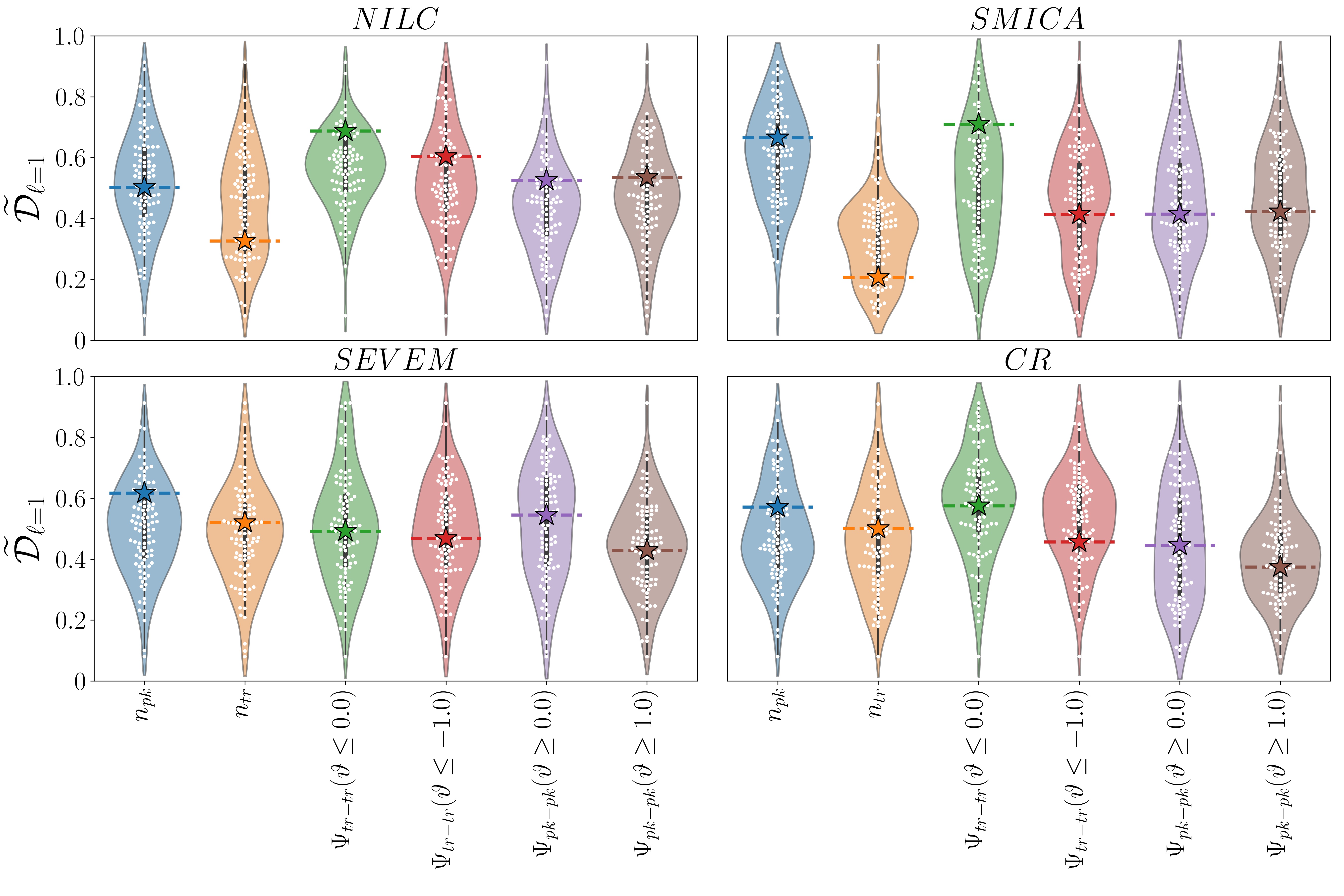
where ${\mathcal{C}}_{\diamond}(\vartheta,\vartheta^{\prime},i,q)\equiv\langle[n^{\rm sim}_{\diamond}(\vartheta,i,q,j)-\langle n^{\rm sim}_{\diamond}(\vartheta,i,q,j)\rangle_{j}][n^{\rm sim}_{\diamond}(\vartheta^{\prime},i,q,j)-\langle n^{\rm sim}_{\diamond}(\vartheta^{\prime},i,q,j)\rangle_{j}]\rangle_{j}$ for each direction. Using the computed $\chi^{2}$ for one-point statistics of local extrema, we construct the associated sky map for each observed maps as well as corresponding simulations. Then, we compute the angular power spectrum for local $\chi_{\diamond}^{2}$ maps. The amplitude of dipole for local $\chi_{\rm pk}^{2}$ and $\chi_{\rm tr}^{2}$ defined by Eq. (4.3) is represented by $\mathcal{D}^{\diamond}_{\ell=1}$ for the Planck maps. For convenience, we normalized computed dipole amplitude to the range of $\widetilde{\mathcal{D}}^{\diamond}_{\ell=1}\in[0,1]$, as illustrated in Fig. 7. In this violin plot, the ‘star’ symbols are associated with observed maps and scattered dots correspond to the simulations. According to the value of angular power spectrum for local $\chi^{2}_{\diamond}$ at $\ell=1$, we compute the probability of obtaining values for the $\mathcal{D}_{\ell=1}^{\diamond}$ for associated simulations at least as large as those given from the observed maps $P(\mathcal{D}^{\diamond}_{\ell=1}>\mathcal{D}^{\diamond,{\rm obs.}}_{\ell=1})$ reported in Table 2. For the unweighted TPCF of local extrema, we also define a local $\chi^{2}_{\diamond-\diamond}(\vartheta,i,q)$ for threshold $\vartheta$, $q$th patch and $i$th map as:

$$\chi^{2}_{\diamond-\diamond}(\vartheta,i,q) = \sum_{m,n}[\Psi_{\diamond-\diamond}(\theta_{m};\vartheta,i,q)-\langle\Psi^{\rm sim}_{\diamond-\diamond}(\theta_{m};\vartheta,i,q,j)\rangle_{j}]$$

$$\times{\mathcal{C}}^{-1}_{\diamond-\diamond}(\theta_{m},\theta_{n};\vartheta,i,q)$$

$$\times[\Psi_{\diamond-\diamond}(\theta_{n};\vartheta,i,q,j)-\langle\Psi^{\rm sim}_{\diamond-\diamond}(\theta_{n};\vartheta,i,q,j)\rangle_{j}]$$

where ${\mathcal{C}}_{\diamond-\diamond,mn}(\vartheta,i,q)\equiv\langle[\Psi^{\rm sim}_{\diamond-\diamond}(\theta_{m};\vartheta,i,q,j)-\langle\Psi^{\rm sim}_{\diamond-\diamond}(\theta_{m};\vartheta,i,q,j)\rangle_{j}][\Psi^{\rm sim}_{\diamond-\diamond}(\theta_{n};\vartheta,i,q,k)-\langle\Psi^{\rm sim}_{\diamond-\diamond}(\theta_{n};\vartheta,i,q,j)\rangle_{k}]\rangle_{jk}$ for each threshold and each direction. The local $\chi^{2}_{\diamond}(\vartheta,i,q)$ for $q$th patch in $i$th map considering different types of measures has been computed. Accordingly, for each measure, a sky map for $\chi_{\diamond}^{2}$ is constructed. Now, we are able to calculate the angular power spectrum for each map. The amplitude power spectra for $\ell=1$ considering different statistical measures are illustrated in Fig. 7. The results for NILC, SMICA, SEVEM and CR have been compared to the results determined for associated simulations in Fig. 7. Table 2 reports the probability of obtaining dipole amplitudes for fiducial map at least as the value given for observed map. Our results show that there is no significant deviation from isotropic field when we use either one- or two-point peak/trough statistics. It is worth noting that, SMICA has different behaviour compared to other observed maps, when we consider clustering of the local trough for $\vartheta\leq 0.0$.

Our statistical measures can be used for identifying probable anomalous patches according to the procedure done by Novaes et al. (2016); Marques et al. (2018).

4.4 Cosmic String Network Detection

A series of phase transitions could have happened in the very early Universe and meanwhile depending on the topology of the potential of the underlying field, we expect to obtain point-like (mono-pole), line-like (cosmic string (CS)), and the texture of topological defects due to spontaneous symmetry breaking in the expanding and cooling Universe (Kibble, 1976, 1980; Hindmarsh & Kibble, 1995; Vilenkin & Shellard, 2000; Copeland & Kibble, 2010; Polchinski, 2005).

In particular, the cosmic string (CS) network is predicted to exist by hybrid inflation, brane-word and superstring theories (Kibble, 1976; Zeldovich, 1980; Vilenkin, 1981; Vachaspati & Vilenkin, 1984; Vilenkin, 1985; Shellard, 1987; Hindmarsh & Kibble, 1995; Vilenkin & Shellard, 2000; Sakellariadou, 2007; Bevis et al., 2008; DePies & Hogan, 2007; Bevis et al., 2010; Copeland et al., 1994; Sakellariadou, 1997; Sarangi & Tye, 2002; Copeland et al., 2004; Pogosian et al., 2003; Majumdar & Christine-Davis, 2002; Dvali & Vilenkin, 2004; Kibble, 2004; Henry Tye, 2008). The energy-density characterization of CS is given by the string tension: $\frac{G\mu}{c^{2}}=\mathcal{O}\!\left(\frac{\varpi^{2}}{M_{\rm Planck}^{2}}\right)$. Here $M_{\rm Planck}\equiv\sqrt{\hbar c/G}$ is the Planck mass, $c$ indicates the speed of light, and $\varpi$ is the energy of symmetry-breaking scale. The search for the footprint of CS network leads to the discovery of proper bounds on $G\mu$ (see Planck Collaboration et al. (2014c); Vafaei Sadr et al. (2017, 2018) and references therein).

To find the upper bound on the CS tension in the Planck data using the local extrema clustering approach, we follow same recipe for the simulation CS-induced CMB map as discussed by Bennett & Bouchet (1990); Ringeval et al. (2007); Fraisse et al. (2008); Vafaei Sadr et al. (2017, 2018). We use high-resolution flat-sky $60^{2}$ deg² patches of CMB maps extended of a full sky simulation for large redshift interval by map stacking method (Bouchet et al., 1988; Ringeval & Bouchet, 2012). The CS tensions used in this work are in the range $2.6\times 10^{-11}\leq G\mu\leq 5.0\times 10^{-7}$ classified into 18 classes for each simulation category. The simulated map for a given $G\mu$ is constructed as $T=T_{\rm Gaussian}+G\mu T_{\rm String}+N$, where $T_{\rm Gaussian}$, $T_{\rm String}$ and $N$ respectively correspond to the end-to-end map associated with each component separation, the normalized string simulated map and the proper noise component. The proper beam effect has been taken into account (Planck Collaboration et al., 2014c). We compare $\Psi_{\rm pk-pk}(\vartheta\geq 0)$ computed for different observations and the one computed for various $G\mu$ simulations.

For a given $G\mu$, we compute the $\Psi_{\rm pk-pk}(\vartheta\geq 0)$ for different observations and for various $G\mu$ simulations. The covariance matrix is also considered as: $\mathcal{C}_{\diamond-\diamond}(\theta_{m},\theta_{n};G\mu,\vartheta,i)\equiv\langle[\Psi_{\diamond-\diamond}^{\rm sim}(\theta_{m};G\mu,\vartheta,i,j)-\langle\Psi_{\diamond-\diamond}^{\rm sim}(\theta_{m};G\mu,\vartheta,i,j)\rangle_{j}][\Psi_{\diamond-\diamond}^{\rm sim}(\theta_{n};G\mu,\vartheta,i,j)-\langle\Psi_{\diamond-\diamond}^{\rm sim}(\theta_{n};G\mu,\vartheta,i,j)\rangle_{j}]\rangle_{j}$, and $\chi^{2}_{\diamond-\diamond}(G\mu,\vartheta,i)$. Now for the observed map, we also determine corresponding $\chi^{2}_{\diamond-\diamond}(\vartheta,i)$. Finally we compare the observation and simulations by checking the inequality as $P_{{\rm C.L.}}\geq\int_{\chi^{2}>\chi^{2}_{\rm pk-pk}(\vartheta)}^{\infty}P(\chi^{2}(G\mu,\vartheta,i))d\chi^{2}(G\mu,\vartheta,i)$. The $P_{{\rm C.L.}}$ is adopted for a given confidence level (C.L.). Therefore, the minimum value of $G\mu$ for which the mentioned inequality is satisfied will be considered by the upper value of CS tension recognized in the observations. We report the $G\mu^{\rm(up)}$ for $\vartheta\geq 0.0$ in Table 3 at $95.5\%$ level of confidence. Comparing our upper bound on CS tension with that of reported by $Planck$ team confirms that taking into account the clustering local extrema achieves almost consistent upper bound determined by considering bispectrum and Minkowski functionals (Planck Collaboration et al., 2014c).

Table 3: The upper bound on the tension of cosmic-strings network, $G\mu^{(\rm up)}$, utilizing $\Psi_{\rm pk-pk}(\vartheta\geq 0)$ as a criterion for recognition.

Map	$G\mu^{(\rm up)}$ (95.5%)
NILC	$8.38\times 10^{-7}$
SEVEM	$6.71\times 10^{-7}$
SMICA	$5.59\times 10^{-7}$
CR	$7.17\times 10^{-7}$

5 Summary and conclusions

The CMB map as a (1+2)-D stochastic field includes thermodynamic temperature and two types of polarization. The mentioned components contain useful information ranging from the early epoch to the late time era. Various physical phenomena have different footprints on the CMB map. The stochastic nature of CMB fluctuations motivates us to rely on geometrical and topological measures to achieve deep insight through the physical mechanisms and associated evolutions. In this paper, we have focused on thermodynamic temperature fluctuations and we addressed the critical sets properties not only in one-point statistics but also in a two-points analysis. After a comprehensive exploration of different research, we turned to the robust perturbative approach to determine the joint PDF of different components of the CMB random field to clarify some examples of excursion and critical sets in the form of one- and two-point statistics. In particular, we derived the perturbative definition of the number density of pixels above a threshold up to $\mathcal{O}(\sigma_{0}^{3})$. By means of the excess probability of finding a typical feature, we computed the unweighted TPCF of local extrema and revisited the semi-analytical definition of the unweighted TPCF of peaks and troughs. In practice, utilizing a semi-analytical approach may encounter the finite-size effect. Therefore we considered three powerful estimators for the rest part of our analysis (Eqs. (2.2), (2.2) and (2.2)).

In order to prepare a robust framework for comparison of the Gaussian prediction and those computed for observed maps, we applied reliable estimators for unweighted TPCF on the Planck fiducial $\Lambda$CDM model (Planck Collaboration et al., 2020a, b) and various component separations as observed by Planck (Planck Collaboration et al., 2020c).

One-point statistics of local extrema and sharp clipping in the form of probability density as a function of threshold and also the cumulative number density function have been computed for both end-to-end simulations and observed Planck temperature CMB maps. Based on the normalized cumulative number density of troughs, we found that NILC and CR represent very tiny deviations from the corresponding simulations around the $\vartheta\in[-2-0]$, while the cumulative number density of peaks confirms the consistency for all component separations. Numbers of peaks, troughs, and sharp clippings for different observed maps compared to the corresponding end-to-end simulated data sets indicated similar results, supporting the Gaussianity hypotheses in the different separation components. However, the pixel statistics at the threshold was less sensitive to the non-Gaussianity. As depicted in Fig. 2, the mean value of the cumulative number density of peaks and troughs for the observed maps is almost higher than the simulations. In addition, the value of the number density of local extrema at $\vartheta\approx 0$ for all observed maps is less than expected in the Gaussian simulation (see Fig. 3).

The unweighted TPCF of local extrema illustrated consistent behaviour in different separation components in all thresholds. For high enough thresholds, the $\Psi_{\rm pk-pk}$ was almost less than the value expected for the fiducial Gaussian simulations. However, the clustering of local extrema reveals good consistency between different component separations (see Fig. 4). Our results revealed that foreground and shot-noise have been excluded in a proper way from different component separations and there is good consistency between the end-to-end simulations and corresponding observed maps when we are dealing with clustering of local extrema. The symmetry behaviour for $\Psi_{\diamond-\diamond}(\delta_{T}\geq\vartheta\sigma_{0})$ and $\Psi_{\diamond-\diamond}(\delta_{T}\leq\vartheta\sigma_{0})$ was confirmed when we considered peaks and troughs rather than pixels reported by Rossi et al. (2009) for WMAP. The value of $\theta$ around the Doppler peak as a function of threshold was decreasing (Fig. 5). Our results demonstrated that, for $\vartheta\sim 0$, we are able to put robust constraint on the amplitude of the mass function according to the value of $\Psi_{\diamond-\diamond}(\theta\approx 70-75)$ arcmin. The scale-independent bias factor for peaks above threshold at high threshold demonstrated $\mathcal{B}_{\rm pk}\sim\vartheta$ which is compatible for sharp clipping in the Gaussian regime, for Planck sets. The scale-dependent part of the bias for peak statistics illustrated some features in the angular scale interval, $20{\rm arcmin}\lesssim\theta\lesssim 80{\rm arcmin}$. For small scales, some deviations between CMB simulated maps and Planck data have been recognized. The higher value of threshold implies the better consistency between $\mathcal{B}_{\rm pk}$ for observed and simulated CMB maps (Fig. 6).

To give quantitative evaluation of non-Gaussianity, we defined the proper $\chi^{2}$ and computed the probability of finding the sample with $\chi^{2}\geq\chi^{2}_{\diamond-\diamond}$ (Table 1). Accordingly, we found that all of statistical measures considered in this paper supported the Gaussian hypothesis.

Asymmetry in the context of $n_{\diamond}$ and $\Psi_{{}_{\diamond-\diamond}}(\theta;\vartheta)$ for patch of $7.5^{2}$ deg² has been examined. The amplitude of the dipole angular spectrum has been computed for all local $\chi^{2}_{\diamond-\diamond}$ (see Fig. 7). The probability of significance of obtaining the asymmetry amplitude, confirmed that all component separations are consistent with the symmetric map (Table 2). The absence of asymmetry significance allowed us to avoid searching for the asymmetry direction in this paper. However, it is useful to evaluate the higher angular power spectrum modes to explore probable anomalies encoded in the clustering of local extrema, which is beyond the scope of the current work. The SMICA map had different behaviour compared to other observed maps when we applied $\Psi_{\rm tr-tr}(\vartheta\leq 0.0)$, however its asymmetry was in agreement with corresponding synthetic data set.

We also derived an upper bound on the cosmic string’s tension via the unweighted TPCF of peaks on the Planck data. The upper bound on the $G\mu$ obtained by peak-peak statistics is almost higher than those bounds derived by other methods; consequently, one concludes that the searching for cosmic strings in the CMB according to the local extrema is very sensitive to even small residual shot-noise in the observations (Table 3). The minimum value of the upper bound was for SMICA map ($G\mu^{(up)}\lesssim 5.59\times 10^{-7}$).

Finally, we remark that it could be interesting to consider crossing statistics (Matsubara, 2003) and construct a complex network from the CMB map to examine the statistical properties and explore probable exotic features such as the cosmic-string network (Albert & Barabási, 2002; Zomorodian, 2016). Topological data analysis under the banner of the homology group is another useful approach in order to achieve the above-mentioned purpose (Zomorodian, 2005; Carlsson, 2009). The implementation of topological and geometrical measures on polarization and convergence maps will be left for our future work.

Data Availability

The new generated data and computational program underlying this article will be shared on reasonable request to the corresponding author.

Appendix A Complementary definitions

In this appendix, we give some complementary definitions used for computing critical sets of the CMB field. The covariance matrix which is represented by Eq. (2.1) is given by:

$$\mathcal{K}^{(2)}\equiv\langle{\mathcal{A}}\otimes{\mathcal{A}}\rangle=\left[\begin{array}[]{cccccc}\langle\delta_{T}^{2}\rangle&\langle\delta_{T}\eta_{\phi}\rangle&\langle\delta_{T}\eta_{\theta}\rangle&\langle\delta_{T}\xi_{\phi\phi}\rangle&\langle\delta_{T}\xi_{\theta\theta}\rangle&\langle\delta_{T}\xi_{\phi\theta}\rangle\\ \langle\delta_{T}\eta_{\phi}\rangle&\langle\eta_{\phi}^{2}\rangle&\langle\eta{\phi}\eta_{\theta}\rangle&\langle\eta{\phi}\xi_{\phi\phi}\rangle&\langle\eta{\phi}\xi_{\theta\theta}\rangle&\langle\eta{\phi}\xi_{\phi\theta}\rangle\\ \langle\delta_{T}\eta_{\theta}\rangle&\langle\eta_{\theta}\eta_{\phi}\rangle&\langle\eta_{\theta}^{2}\rangle&\langle\eta_{\theta}\xi_{\phi\phi}\rangle&\langle\eta_{\theta}\xi_{\theta\theta}\rangle&\langle\eta_{\theta}\xi_{\phi\theta}\rangle\\ \langle\delta_{T}\xi_{\phi\phi}\rangle&\langle\xi_{\phi\phi}\eta_{\phi}\rangle&\langle\xi_{\phi\phi}\eta_{\theta}\rangle&\langle\xi_{\phi\phi}^{2}\rangle&\langle\xi_{\phi\phi}\xi_{\theta\theta}\rangle&\langle\xi_{\phi\phi}\xi_{\phi\theta}\rangle\\ \langle\delta_{T}\xi_{\theta\theta}\rangle&\langle\xi_{\theta\theta}\eta_{\phi}\rangle&\langle\xi_{\theta\theta}\eta_{\theta}\rangle&\langle\xi_{\theta\theta}\xi_{\phi\phi}\rangle&\langle\xi_{\theta\theta}^{2}\rangle&\langle\xi_{\theta\theta}\xi_{\phi\theta}\rangle\\ \langle\delta_{T}\xi_{\phi\theta}\rangle&\langle\xi_{\phi\theta}\eta_{\phi}\rangle&\langle\xi_{\phi\theta}\eta_{\theta}\rangle&\langle\xi_{\phi\theta}\xi_{\phi\phi}\rangle&\langle\xi_{\phi\theta}\xi_{\theta\theta}\rangle&\langle\xi_{\phi\theta}^{2}\rangle\\ \end{array}\right]$$ (24)

The non-zero elements of $\mathcal{K}^{(2)}$ for separation angle, $\cos(\psi)=|\hat{n}_{i}.\hat{n}_{j}|=1$ are as follows (Bond & Efstathiou, 1987):

$$\sigma_{0}^{2} \equiv \langle\delta_{T}^{2}\rangle=\sum_{\ell}\frac{(2\ell+1)}{4\pi}C^{TT}_{\ell}W^{2}_{\ell}$$ (25)

$$\langle\delta_{T}\xi_{\phi\phi}\rangle = \langle\delta_{T}\xi_{\theta\theta}\rangle=-\sum_{\ell}\frac{(2\ell+1)}{4\pi}\frac{\ell(\ell+1)}{2}C^{TT}_{\ell}W^{2}_{\ell}$$

$$\langle\xi_{\theta\theta}^{2}\rangle = \sum_{\ell}\frac{(2\ell+1)}{4\pi}\frac{(3\ell(\ell+1)-2)\ell(\ell+1)}{8}C^{TT}_{\ell}W^{2}_{\ell}$$

$$\langle\xi_{\theta\theta}\xi_{\phi\phi}\rangle = \sum_{\ell}\frac{(2\ell+1)}{4\pi}\frac{(\ell(\ell+1)+2)\ell(\ell+1)}{8}C^{TT}_{\ell}W^{2}_{\ell}$$

$$\langle\xi_{\phi\theta}^{2}\rangle = \sum_{\ell}\frac{(2\ell+1)}{4\pi}\frac{(\ell+2)(\ell+1)\ell(\ell-1)}{8}C^{TT}_{\ell}W^{2}_{\ell}$$

where $W_{\ell}=\exp\left(-\theta_{\rm beam}^{2}\ell(\ell+1)/2\right)$ and $\theta_{\rm beam}\equiv\theta_{\rm FWHM}/\sqrt{8\ln(2)}$ for a Gaussian smoothing kernel associated with beam transfer function (Bond & Efstathiou, 1987; Heavens & Sheth, 1999; Hikage et al., 2006). Also $C^{TT}_{\ell}$ is the power spectrum of CMB temperature fluctuations. Other terms are $\langle\eta_{\phi}^{2}\rangle=\langle\eta_{\theta}^{2}\rangle=-\langle\delta_{T}\xi_{\phi\phi}\rangle$ and $\langle\xi_{\theta\theta}^{2}\rangle=\langle\xi_{\phi\phi}^{2}\rangle$.

References

- Adhikari et al. (2018) Adhikari S., Deutsch A.-S., Shandera S., 2018, Physical Review D, 98, 023520
- Adler (1981) Adler R., 1981, The Geometry of Random Fields, Chichester: Wiley, 1981
- Adler & Taylor (2011) Adler R., Taylor J. E., 2011, Topological Complexity of Smooth Random Functions: École D’Été de Probabilités de Saint-Flour XXXIX-2009. Springer Science & Business Media
- Adler et al. (2010) Adler R. J., Bobrowski O., Borman M. S., Subag E., Weinberger S., et al., 2010, in , Borrowing strength: theory powering applications–a Festschrift for Lawrence D. Brown. Institute of Mathematical Statistics, pp 124–143
- Akrami et al. (2014) Akrami Y., Fantaye Y., Shafieloo A., Eriksen H., Hansen F. K., Banday A. J., Górski K. M., 2014, The Astrophysical Journal Letters, 784, L42
- Albert & Barabási (2002) Albert R., Barabási A.-L., 2002, Reviews of modern physics, 74, 47
- Bardeen et al. (1986) Bardeen J. M., Bond J. R., Kaiser N., Szalay A. S., 1986, Astrophys. J., 304, 15
- Barreiro et al. (1997) Barreiro R., Sanz J., Martínez-González E., Cayón L., Silk J., 1997, The Astrophysical Journal, 478, 1
- Bennett & Bouchet (1990) Bennett D. P., Bouchet F. R., 1990, Physical Review D, 41, 2408
- Bernardeau et al. (2002) Bernardeau F., Colombi S., Gaztanaga E., Scoccimarro R., 2002, Physics reports, 367, 1
- Bevis et al. (2008) Bevis N., Hindmarsh M., Kunz M., Urrestilla J., 2008, Phys. Rev. Lett., 100, 021301
- Bevis et al. (2010) Bevis N., Hindmarsh M., Kunz M., Urrestilla J., 2010, Phys. Rev., D82, 065004
- Bond & Efstathiou (1987) Bond J., Efstathiou G., 1987, Monthly Notices of the Royal Astronomical Society, 226, 655
- Borgani (1995) Borgani S., 1995, Physics Reports, 251, 1
- Bouchet et al. (1988) Bouchet F. R., Bennett D. P., Stebbins A., 1988, Nature, 335, 410
- Brill (2000) Brill P. H., 2000, CORS Bulletin, 34, 9
- Buchert et al. (2017) Buchert T., France M. J., Steiner F., 2017, Classical and Quantum Gravity, 34, 094002
- Carlsson (2009) Carlsson G., 2009, Bulletin of the American Mathematical Society, 46, 255
- Cayon & Smoot (1995) Cayon L., Smoot G., 1995, The Astrophysical Journal, 452, 487
- Codis et al. (2013) Codis S., Pichon C., Pogosyan D., Bernardeau F., Matsubara T., 2013, Monthly Notices of the Royal Astronomical Society, 435, 531
- Cole & Shiu (2018) Cole A., Shiu G., 2018, Journal of Cosmology and Astroparticle Physics, 2018, 025
- Colley & Gott III (2015) Colley W. N., Gott III J. R., 2015, Monthly Notices of the Royal Astronomical Society, 447, 2034
- Colley & Richard Gott III (2003) Colley W. N., Richard Gott III J., 2003, Monthly Notices of the Royal Astronomical Society, 344, 686
- Cooray & Sheth (2002) Cooray A., Sheth R., 2002, Physics Reports, 372, 1
- Copeland & Kibble (2010) Copeland E. J., Kibble T. W. B., 2010, Proc. Roy. Soc. Lond., A466, 623
- Copeland et al. (1994) Copeland E. J., Liddle A. R., Lyth D. H., Stewart E. D., Wands D., 1994, Phys. Rev., D49, 6410
- Copeland et al. (2004) Copeland E. J., Myers R. C., Polchinski J., 2004, JHEP, 06, 013
- Copi et al. (2004) Copi C. J., Huterer D., Starkman G. D., 2004, Physical Review D, 70, 043515
- Copi et al. (2006) Copi C. J., Huterer D., Schwarz D. J., Starkman G. D., 2006, Monthly Notices of the Royal Astronomical Society, 367, 79
- Davis & Peebles (1983) Davis M., Peebles P., 1983, The Astrophysical Journal, 267, 465
- DePies & Hogan (2007) DePies M. R., Hogan C. J., 2007, Physical Review D, 75, 125006
- Desjacques et al. (2010) Desjacques V., Crocce M., Scoccimarro R., Sheth R. K., 2010, Physical Review D, 82, 103529
- Desjacques et al. (2018) Desjacques V., Jeong D., Schmidt F., 2018, Physics reports, 733, 1
- Dickinson (2016) Dickinson C., 2016, arXiv preprint arXiv:1606.03606
- Dodelson (2003) Dodelson S., 2003, Modern cosmology. Academic press
- Doré et al. (2003) Doré O., Colombi S., Bouchet F. R., 2003, Monthly Notices of the Royal Astronomical Society, 344, 905
- Dvali & Vilenkin (2004) Dvali G., Vilenkin A., 2004, JCAP, 0403, 010
- Eriksen et al. (2004) Eriksen H. K., Hansen F. K., Banday A. J., Górski K. M., Lilje P. B., 2004, The Astrophysical Journal, 605, 14
- Fabbri & Torres (1996) Fabbri R., Torres S., 1996, Astronomy and Astrophysics, 307, 703
- Fang et al. (2017) Fang W., Li B., Zhao G.-B., 2017, Physical review letters, 118, 181301
- Fraisse et al. (2008) Fraisse A. A., Ringeval C., Spergel D. N., Bouchet F. R., 2008, Physical Review D, 78, 043535
- Futamase & Takada (2000) Futamase T., Takada M., 2000, arXiv preprint astro-ph/0009153
- Gay et al. (2012) Gay C., Pichon C., Pogosyan D., 2012, Physical Review D, 85, 023011
- Ghasemi Nezhadhaghighi et al. (2017) Ghasemi Nezhadhaghighi M., Movahed S., Yasseri T., Vaez Allaei S. M., 2017, Journal of Applied Physics, 122, 085302
- Ghasemi et al. (2006) Ghasemi F., Bahraminasab A., Movahed M. S., Rahvar S., Sreenivasan K., Tabar M. R. R., 2006, Journal of Statistical Mechanics: Theory and Experiment, 2006, P11008
- Gorski et al. (2005) Gorski K. M., Hivon E., Banday A., Wandelt B. D., Hansen F. K., Reinecke M., Bartelmann M., 2005, The Astrophysical Journal, 622, 759
- Gott et al. (2007) Gott III J. R., Colley W. N., Park C.-G., Park C., Mugnolo C., 2007, Mon. Not. Roy. Astron. Soc., 377, 1668
- Hadwiger (2013) Hadwiger H., 2013, Vorlesungen über inhalt, Oberfläche und isoperimetrie. Vol. 93, Springer-Verlag
- Hajian & Souradeep (2003) Hajian A., Souradeep T., 2003, The Astrophysical Journal Letters, 597, L5
- Hajian & Souradeep (2006) Hajian A., Souradeep T., 2006, Physical Review D, 74, 123521
- Hamilton (1993) Hamilton A., 1993, The Astrophysical Journal, 417, 19
- Hansen et al. (2009) Hansen F., Banday A., Górski K., Eriksen H., Lilje P., 2009, The Astrophysical Journal, 704, 1448
- Hanson & Lewis (2009) Hanson D., Lewis A., 2009, Physical Review D, 80, 063004
- Heavens & Gupta (2001) Heavens A. F., Gupta S., 2001, Monthly Notices of the Royal Astronomical Society, 324, 960
- Heavens & Sheth (1999) Heavens A. F., Sheth R. K., 1999, Monthly Notices of the Royal Astronomical Society, 310, 1062
- Henry Tye (2008) Henry Tye S. H., 2008, Lect. Notes Phys., 737, 949
- Hernández-Monteagudo et al. (2004) Hernández-Monteagudo C., Kashlinsky A., Atrio-Barandela F., 2004, Astronomy & Astrophysics, 413, 833
- Hewett (1982) Hewett P. C., 1982, Monthly Notices of the Royal Astronomical Society, 201, 867
- Hikage et al. (2006) Hikage C., Komatsu E., Matsubara T., 2006, The Astrophysical Journal, 653, 11
- Hindmarsh & Kibble (1995) Hindmarsh M. B., Kibble T. W. B., 1995, Rept. Prog. Phys., 58, 477
- Hoftuft et al. (2009) Hoftuft J., Eriksen H., Banday A., Gorski K., Hansen F., Lilje P., 2009, The Astrophysical Journal, 699, 985
- Hou et al. (2009) Hou Z., Banday A. J., Górski K. M., 2009, MNRAS, 396, 1273
- Jensen & Szalay (1986) Jensen L. G., Szalay A., 1986, The Astrophysical Journal, 305, L5
- Kaiser (1984) Kaiser N., 1984, The Astrophysical Journal, 284, L9
- Kashlinsky (2005) Kashlinsky A., 2005, Physics Reports, 409, 361
- Kashlinsky et al. (2001) Kashlinsky A., Hernández-Monteagudo C., Atrio-Barandela F., 2001, The Astrophysical Journal Letters, 557, L1
- Kerscher et al. (2000) Kerscher M., Szapudi I., Szalay A. S., 2000, The Astrophysical Journal Letters, 535, L13
- Kibble (1976) Kibble T. W. B., 1976, J. Phys., A9, 1387
- Kibble (1980) Kibble T. W. B., 1980, Phys. Rept., 67, 183
- Kibble (2004) Kibble T. W., 2004, arXiv preprint astro-ph/0410073
- Kogut et al. (1995) Kogut A. J., Banday A. J., Bennett C. L., Hinshaw G. F., Lubin P. M., Smoot G. F., 1995, Astrophysical Journal, 439, 29
- Kogut et al. (1996) Kogut A., Banday A. J., Bennett C. L., Górski K. M., Hinshaw G., Smoot G. F., Wright E. L., 1996, The Astrophysical Journal Letters, 464, L29
- Komatsu (2002) Komatsu E., 2002, arXiv preprint astro-ph/0206039
- Landy & Szalay (1993) Landy S. D., Szalay A. S., 1993, Astrophys. J., 412, 64
- Larson & Wandelt (2004) Larson D. L., Wandelt B. D., 2004, ApJ, 613, L85
- Larson & Wandelt (2005) Larson D. L., Wandelt B. D., 2005, arXiv preprint astro-ph/0505046
- Lesgourges (2013) Lesgourges J., 2013, in , Searching for New Physics at Small and Large Scales: TASI 2012. World Scientific, pp 29–97
- Lesgourgues et al. (2013) Lesgourgues J., Mangano G., Miele G., Pastor S., 2013, Neutrino cosmology. Cambridge University Press
- Lewis & Challinor (2006) Lewis A., Challinor A., 2006, Physics Reports, 429, 1
- Ling et al. (2015) Ling C., Wang Q., Li R., Li B., Wang J., Gao L., 2015, Physical Review D, 92, 064024
- Lumsden et al. (1989) Lumsden S., Heavens A., Peacock J., 1989, Monthly Notices of the Royal Astronomical Society, 238, 293
- Majumdar & Christine-Davis (2002) Majumdar M., Christine-Davis A., 2002, JHEP, 03, 056
- Malik & Wands (2009) Malik K. A., Wands D., 2009, Phys. Rept., 475, 1
- Marcos-Caballero et al. (2016) Marcos-Caballero A., Fernández-Cobos R., Martínez-González E., Vielva P., 2016, JCAP, 04, 058
- Marques et al. (2018) Marques G., Novaes C., Bernui A., Ferreira I., 2018, Monthly Notices of the Royal Astronomical Society, 473, 165
- Martinez & Saar (2001) Martinez V. J., Saar E., 2001, Statistics of the galaxy distribution. CRC press
- Matsubara (1996) Matsubara T., 1996, The Astrophysical Journal, 457, 13
- Matsubara (2003) Matsubara T., 2003, The Astrophysical Journal, 584, 1
- Matsubara (2010) Matsubara T., 2010, Physical Review D, 81, 083505
- Matsubara (2020) Matsubara T., 2020, Physical Review D, 101, 043532
- Mecke et al. (1994) Mecke K., Bucheri T., Wagner H., 1994, Astron. Astrophys, 288, 697
- Movahed & Khosravi (2011) Movahed M. S., Khosravi S., 2011, Journal of Cosmology and Astroparticle Physics, 2011, 012
- Movahed et al. (2011) Movahed M. S., Ghasemi F., Rahvar S., Tabar M. R. R., 2011, Physical Review E, 84, 021103
- Movahed et al. (2013) Movahed M. S., Javanmardi B., Sheth R. K., 2013, Monthly Notices of the Royal Astronomical Society, 434, 3597
- Novaes et al. (2016) Novaes C., Bernui A., Marques G., Ferreira I., 2016, Monthly Notices of the Royal Astronomical Society, 461, 1363
- Peacock & Heavens (1985) Peacock J., Heavens A. F., 1985, Monthly Notices of the Royal Astronomical Society, 217, 805
- Peebles (1980) Peebles P. J. E., 1980, The large-scale structure of the universe. Princeton university press
- Planck Collaboration et al. (2014a) Planck Collaboration et al., 2014a, A&A, 571, A23
- Planck Collaboration et al. (2014b) Planck Collaboration et al., 2014b, A&A, 571, A24
- Planck Collaboration et al. (2014c) Planck Collaboration et al., 2014c, A&A, 571, A25
- Planck Collaboration et al. (2016a) Planck Collaboration et al., 2016a, A&A, 594, A9
- Planck Collaboration et al. (2016b) Planck Collaboration et al., 2016b, A&A, 594, A13
- Planck Collaboration et al. (2016c) Planck Collaboration et al., 2016c, A&A, 594, A16
- Planck Collaboration et al. (2016d) Planck Collaboration et al., 2016d, A&A, 594, A17
- Planck Collaboration et al. (2020a) Planck Collaboration et al., 2020a, A&A, 641, A2
- Planck Collaboration et al. (2020b) Planck Collaboration et al., 2020b, A&A, 641, A3
- Planck Collaboration et al. (2020c) Planck Collaboration et al., 2020c, A&A, 641, A4
- Planck Collaboration et al. (2020d) Planck Collaboration et al., 2020d, A&A, 641, A6
- Planck Collaboration et al. (2020e) Planck Collaboration et al., 2020e, A&A, 641, A7
- Planck Collaboration et al. (2020f) Planck Collaboration et al., 2020f, A&A, 641, A9
- Pogosian et al. (2003) Pogosian L., Tye S.-H. H., Wasserman I., Wyman M., 2003, Physical Review D, 68, 023506
- Pogosyan et al. (2009) Pogosyan D., Pichon C., Gay C., Prunet S., Cardoso J., Sousbie T., Colombi S., 2009, Monthly Notices of the Royal Astronomical Society, 396, 635
- Pogosyan et al. (2011) Pogosyan D., Pichon C., Gay C., 2011, Physical Review D, 84, 083510
- Polchinski (2005) Polchinski J., 2005, Int. J. Mod. Phys., A20, 3413
- Politzer & Wise (1984) Politzer H. D., Wise M. B., 1984, The Astrophysical Journal, 285, L1
- Pranav et al. (2019) Pranav P., et al., 2019, Monthly Notices of the Royal Astronomical Society, 485, 4167
- Prunet et al. (2005) Prunet S., Uzan J.-P., Bernardeau F., Brunier T., 2005, Physical Review D, 71, 083508
- Rath & Jain (2013) Rath P. K., Jain P., 2013, Journal of Cosmology and Astroparticle Physics, 2013, 014
- Rath et al. (2013) Rath P. K., Mudholkar T., Jain P., Aluri P. K., Panda S., 2013, Journal of Cosmology and Astroparticle Physics, 2013, 007
- Rath et al. (2018) Rath P. K., Samal P. K., Panda S., Mishra D. D., Aluri P. K., 2018, Monthly Notices of the Royal Astronomical Society, 475, 4357
- Reischke et al. (2015) Reischke R., Maturi M., Bartelmann M., 2015, Monthly Notices of the Royal Astronomical Society, 456, 641
- Renaux-Petel (2015) Renaux-Petel S., 2015, Comptes Rendus Physique, 16, 969
- Rice (1944) Rice S. O., 1944, Bell Labs Technical Journal, 23, 282
- Rice (1945) Rice S. O., 1945, The Bell System Technical Journal, 24, 46
- Rice (1954) Rice S., 1954, ed. N. Wax, Dover Publ. Inc.(NY)
- Ringeval & Bouchet (2012) Ringeval C., Bouchet F. R., 2012, Physical Review D, 86, 023513
- Ringeval et al. (2007) Ringeval C., Sakellariadou M., Bouchet F. R., 2007, Journal of Cosmology and Astroparticle Physics, 2007, 023
- Rossi (2013) Rossi G., 2013, Monthly Notices of the Royal Astronomical Society, 430, 1486
- Rossi et al. (2009) Rossi G., Sheth R. K., Park C., Hernández-Monteagudo C., 2009, Monthly Notices of the Royal Astronomical Society, 399, 304
- Rossi et al. (2011) Rossi G., Chingangbam P., Park C., 2011, Monthly Notices of the Royal Astronomical Society, 411, 1880
- Ryden (1988) Ryden B. S., 1988, The Astrophysical Journal, 333, L41
- Ryden et al. (1989) Ryden B. S., Melott A. L., Craig D. A., Gott III J. R., Weinberg D. H., Scherrer R. J., Bhavsar S. P., Miller J. M., 1989, The Astrophysical Journal, 340, 647
- Sakellariadou (1997) Sakellariadou M., 1997, Int. J. Theor. Phys., 36, 2503
- Sakellariadou (2007) Sakellariadou M., 2007, Lect. Notes Phys., 718, 247
- Sarangi & Tye (2002) Sarangi S., Tye S. H. H., 2002, Phys. Lett., B536, 185
- Sazhin (1985) Sazhin M., 1985, Monthly Notices of the Royal Astronomical Society, 216, 25P
- Schmalzing & Górski (1998) Schmalzing J., Górski K. M., 1998, Monthly Notices of the Royal Astronomical Society, 297, 355
- Schmalzing et al. (1995) Schmalzing J., Buchert T., Kerscher M., 1995, Proc. Int. Sch. Phys. Fermi, 132, 281
- Shahbazi et al. (2003) Shahbazi F., Sobhanian S., Tabar M. R. R., Khorram S., Frootan G., Zahed H., 2003, Journal of Physics A: Mathematical and General, 36, 2517
- Shellard (1987) Shellard E. P. S., 1987, Nucl. Phys., B283, 624
- Szalay (1988a) Szalay A. S., 1988a, in Symposium-International Astronomical Union. pp 163–167
- Szalay (1988b) Szalay A. S., 1988b, The Astrophysical Journal, 333, 21
- Takada & Futamase (2001) Takada M., Futamase T., 2001, The Astrophysical Journal, 546, 620
- Takada et al. (2000) Takada M., Komatsu E., Futamase T., 2000, The Astrophysical Journal Letters, 533, L83
- Taqqu (1977) Taqqu M. S., 1977, Probability Theory and Related Fields, 40, 203
- Tojeiro et al. (2006) Tojeiro R., Castro P., Heavens A., Gupta S., 2006, Monthly Notices of the Royal Astronomical Society, 365, 265
- Vachaspati & Vilenkin (1984) Vachaspati T., Vilenkin A., 1984, Physical Review D, 30, 2036
- Vafaei Sadr et al. (2017) Vafaei Sadr A., Movahed S., Farhang M., Ringeval C., Bouchet F., 2017, Monthly Notices of the Royal Astronomical Society, 475, 1010
- Vafaei Sadr et al. (2018) Vafaei Sadr A., Farhang M., Movahed S., Bassett B., Kunz M., 2018, Monthly Notices of the Royal Astronomical Society, 478, 1132
- Vilenkin (1981) Vilenkin A., 1981, Phys. Rev. Lett., 46, 1169
- Vilenkin (1985) Vilenkin A., 1985, Phys. Rept., 121, 263
- Vilenkin & Shellard (2000) Vilenkin A., Shellard E. P. S., 2000, Cosmic strings and other topological defects. Cambridge University Press
- Vittorio & Juszkiewicz (1987) Vittorio N., Juszkiewicz R., 1987, The Astrophysical Journal, 314, L29
- Zeldovich (1980) Zeldovich Ya. B., 1980, Mon. Not. Roy. Astron. Soc., 192, 663
- Zomorodian (2005) Zomorodian A. J., 2005, Topology for computing. Cambridge university press
- Zomorodian (2016) Zomorodian A. J., 2016, Network science. Cambridge university press