Learning Driver Behaviors Using A Gaussian Process Augmented State-Space Model
Abstract
An inference method for Gaussian process augmented state-space models are presented. This class of grey-box models enables domain knowledge to be incorporated in the inference process to guarantee a minimum of performance, still they are flexible enough to permit learning of partially unknown model dynamics and inputs. To facilitate online (recursive) inference of the model a sparse approximation of the Gaussian process based upon inducing points is presented. To illustrate the application of the model and the inference method, an example where it is used to track the position and learn the behavior of a set of cars passing through an intersection, is presented. Compared to the case when only the state-space model is used, the use of the augmented state-space model gives both a reduced estimation error and bias.
I Introduction
State estimation is a fundamental problem in many areas, such as robotics, target tracking, economics, etc. Typical techniques for state estimation are Bayesian filters such as the Kalman Filter (kf), Extended Kalman Filter (ekf) or the Particle Filter (pf) [1]. Common to these techniques is that they require a model for the state dynamics as well as an observation model for the considered system. A general model for this is
| (1a) | ||||
| (1b) | ||||
where and are the state dynamics and observation model, respectively, and can be both time-varying and nonlinear. Further, is the state vector at time , is some input, and and are mutually independent Gaussian white noise with covariance matrices and , respectively. Commonly, and are chosen based upon insight about the underlying physical process and the sensors used to observe it [2].
If information about the underlying process is missing, a model can be inferred from data using system identification methods [2]. This can for instance be done using a Gaussian Process State-Space Model (gpssm), where both the state dynamics and observation model are viewed as separate Gaussian Processes (gps) and learned jointly [3, 4, 5, 6, 7]. These methods may include prior physical knowledge, but only through the prior mean and is thus not so flexible. Moreover, they are computationally demanding and not well suited for online application.
I-A Augmented State-Space Models
In many situations, knowledge about parts of the underlying process might exist, or a simplified model of the process exists. One way to incorporate this knowledge into the state estimation problem is to separate the system into two parts, one known (here assumed linear) and one unknown part, where the unknown part is modeled as a gp [8]. That is,
| (2a) | |||
| (2b) | |||
| (2c) | |||
Here, is an unknown input at time , which is to be inferred from data. It depends on some variable , which may change over time. For example, could be a function of the state . Furthermore, the input is modeled as a gp but could also, e.g., be a basis function expansion or neural network [9, 10]. Henceforth, the model (2) will be referred to as a Gaussian Process Augmented State-Space Model (gpassm). The benefits of this class of grey-box models are that they provide:
-
1.
Performance guarantees — the model will perform at least as well as the simplified state dynamics model.
-
2.
Interpretability of — in many cases, the learned inputs have a meaningful, physical interpretation.
-
3.
Improvement over time — as more data is available, the model accuracy improves and so also the state estimation accuracy.
-
4.
Information sharing — if many systems behave similarly, the input may be shared between systems and learned jointly.
This class of models could for instance be exploited for tracking ships, or icebergs, where the learned input could be interpreted as the ocean currents [8]. It could also be used for estimating the structural integrity of buildings which is affected by unknown outer forces, which could be learned [11]. A final example is predicting the number of remaining charging cycles of batteries. In Lithium-Ion batteries it is well understood that the usage history and environment affect the degradation process [12]. These effects can potentially be learned from other batteries with similar history to accurately predict degradation and schedule maintenance accordingly.
I-B Scenario Description
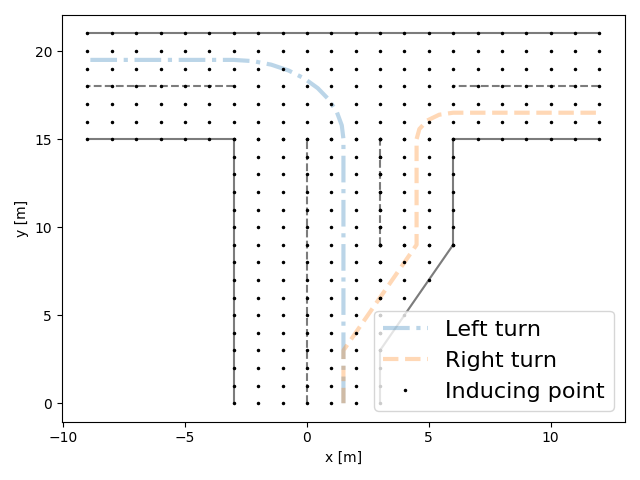
Before an estimator for the gpassm is derived, a usage scenario is presented to give a foundation for the forthcoming discussion. The considered scenario is visualized in Fig 1. A vehicle approaches the intersection from the middle road and travels through the intersection according to one of the two possible paths. The problem is to estimate the state of the vehicle given by
| (3) |
where and is the position and velocity along the :th-axis, respectively. In a typical vehicle tracking application, the information provided by its trajectory is forgotten and the trajectory of each new vehicle passing through the intersection is assumed independent from its predecessors. In scenarios such as that illustrated by Fig 1, this assumption is naive since each vehicle in the intersection are bound to follow traffic regulations, the road network, etc. Hence, there will be a high correlation between the dynamics of the vehicles that pass through the intersection. This dynamic can be modeled as an unknown input to the model of the vehicles’ motion and can be learned by sharing information between vehicles. To that end, the motion dynamics of the vehicles will be modeled by a gpassm where the known model dynamics is given by a Constant Velocity (cv) model [13], and the unknown driver input, i.e., the accelerations, are modeled by a gp.
II Modeling
In its basic form, the gpassm presented in (2) cannot be used for online learning and state estimation as the inference of the gp increases cubically with the number of observations [14]. Therefore, we will next introduce a sparse approximation for the Gaussian process and modify the model gpassm accordingly. For simplicity, but without loss of generality, the observation function will be assumed linear.
II-A Approximating the input
There has been a lot of research in approximating gp regression, both in the static cases where all of the data is available at training time, as well as in the dynamic case where the data is added over time. These approximations can be divided into two distinct tracks, inducing inputs and basis function expansion. A comprehensive review of inducing input approaches can be found in [15]. An introduction to basis function expansion can be found in [14, 3, 16, 17].
Here, each gp will be approximated using inducing inputs, which is a set of discrete points fixed at some arbitrary location. Here, the points are fixed at for and their corresponding function values are given by and are referred to as inducing inputs. Gather the inducing inputs in the vector and their corresponding coordinates in . Next, let
| (4) | ||||
| (5) | ||||
| (6) |
where is the identity matrix. If the inputs are assumed independent of each other and the same kernel is used for each input , the complete covariance matrix for is given by . By using the Fully Independent Conditional (fic) approximation [15, 18], the model can now be written as
| (7a) | ||||
| (7b) | ||||
| (7c) | ||||
where is Gaussian white noise with covariance matrix . Hence, the input at a given point is given by a linear combination of the inducing inputs. Lastly, the matrix is not always well conditioned so to avoid numerical issues define
| (8) |
and note that
which is only needed for interpreting the covariance of the estimates and is not necessary for implementing the estimation. To allow the model to adapt to changes in the input, the inducing point state will be modeled as a random walk process. That is,
| (9) |
where is Gaussian white noise with covariance matrix . The state vector is then augmented with and the model becomes
| (10a) | ||||
| (10b) | ||||
| (10c) | ||||
and note that still depends on the parameters .
II-B State-dependent input
In the considered scenario, the vehicle acceleration depends on the location of the vehicle within the intersection. Hence, the input depends on the position of the vehicle, i.e.,
| (11a) | ||||
| (11b) | ||||
The acceleration of course also depends on the velocity of the vehicle (The centripetal acceleration through a curve is given by , where is the radius of the curve and is the absolute speed.). However, as this would quadratically scale the inducing point space (from to ), this is neglected for computational reasons. The full model is then described by
| (12a) | ||||
| (12b) | ||||
| (12c) | ||||
| (12d) | ||||
Recall that and note that the model is now nonlinear in the states due to the dependence of on .
II-C Kernel choice
The choice of kernel function specifies what family of functions the gp is able to approximate well [14]. A common choice is the squared exponential kernel
| (13) |
which will be used here as well. The hyperparameters govern the properties of the kernel, where controls the general variance and is the characteristic length-scale and controls the width of the kernel. The hyperparameters can either be learned online [19], [20] or selected manually based on insight about the physical properties of the input.
III Estimation
The model (12) is nonlinear in the states and can be recursively estimated using, e.g., an ekf based on a first order Taylor expansion [1]. The ekf assumes that the prediction and filter distributions are both normally distributed as
| (14) | ||||
| (15) |
By using the upper triangular structure of the state transition model (12a) and (12b), the ekf time-update becomes [8]
| (16a) | ||||
| (16b) | ||||
| (16c) | ||||
| (16d) | ||||
| (16e) | ||||
| (16f) | ||||
and the measurement update becomes
| (17a) | ||||
| (17b) | ||||
| (17c) | ||||
| (17d) | ||||
| (17e) | ||||
| (17f) | ||||
| (17g) | ||||
| (17h) | ||||
| (17i) | ||||
where
| (18) | ||||
| (19) |
See Appendix A for a derivation.
IV Simulation and Results
To illustrate the application of the proposed estimation approach and the gpassm, position observations from a set of vehicles passing through the intersection illustrated in Fig 1 were simulated.
IV-A Simulation Parameters
There are a number of parameters to be either learned or chosen. Here, they are all manually selected based on prior knowledge of the physical properties of the scenario. For the vehicle motion, a cv is chosen, i.e.,
| (20) |
where is the sampling interval. For the observation model, it is assumed that the position of the vehicle is measurable with some noise, i.e.,
| (21) |
where is the measurement noise variance.
As for the gp, there are three parameters to be chosen: the location of the inducing points , the kernel variance , and the kernel length scale . The inducing points are fixed on a grid covering the entire intersection, see Fig 1, uniformly spaced using a grid spacing , which was chosen as a trade-off between accuracy and computational burden. The kernel variance and length scale are chosen under the notion that the acceleration of a vehicle is a local phenomena and varies quickly over distance/time. The length scale is thus chosen as and the variance as . The simulation parameters are summarized in Table I.
During the simulations, all the vehicles were initiated to the true initial position and velocity. In total simulations were run.
| Parameter | Description | Value |
| L | # Inducing points | 310 |
| N | # Vehicles | 30 |
| Sampling rate | ||
| Measurement noise variance | 0.2 | |
| Kernel variance | 0.05 | |
| Kernel length scale | 0.5 | |
| R | ekf measurement noise variance | 1 |
| Grid spacing |
IV-B Qualitative Analysis
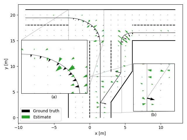
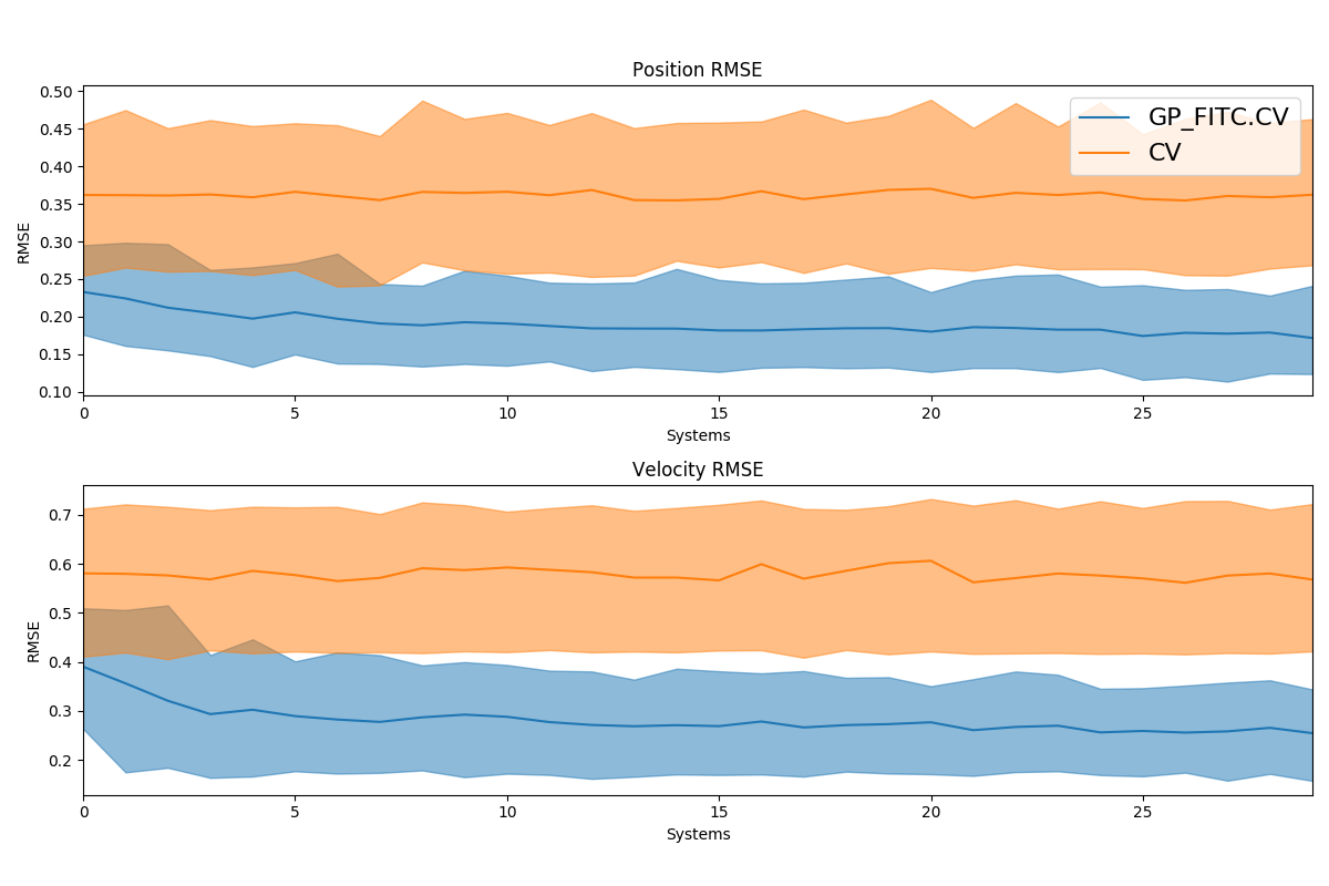
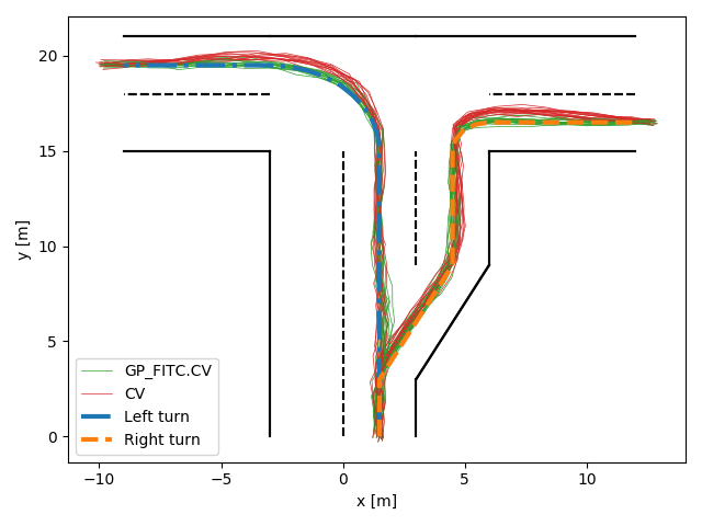
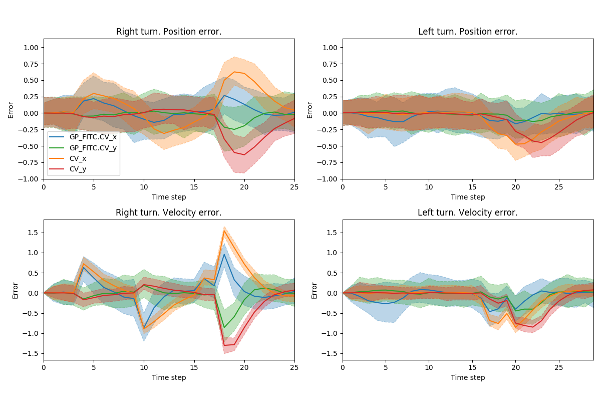
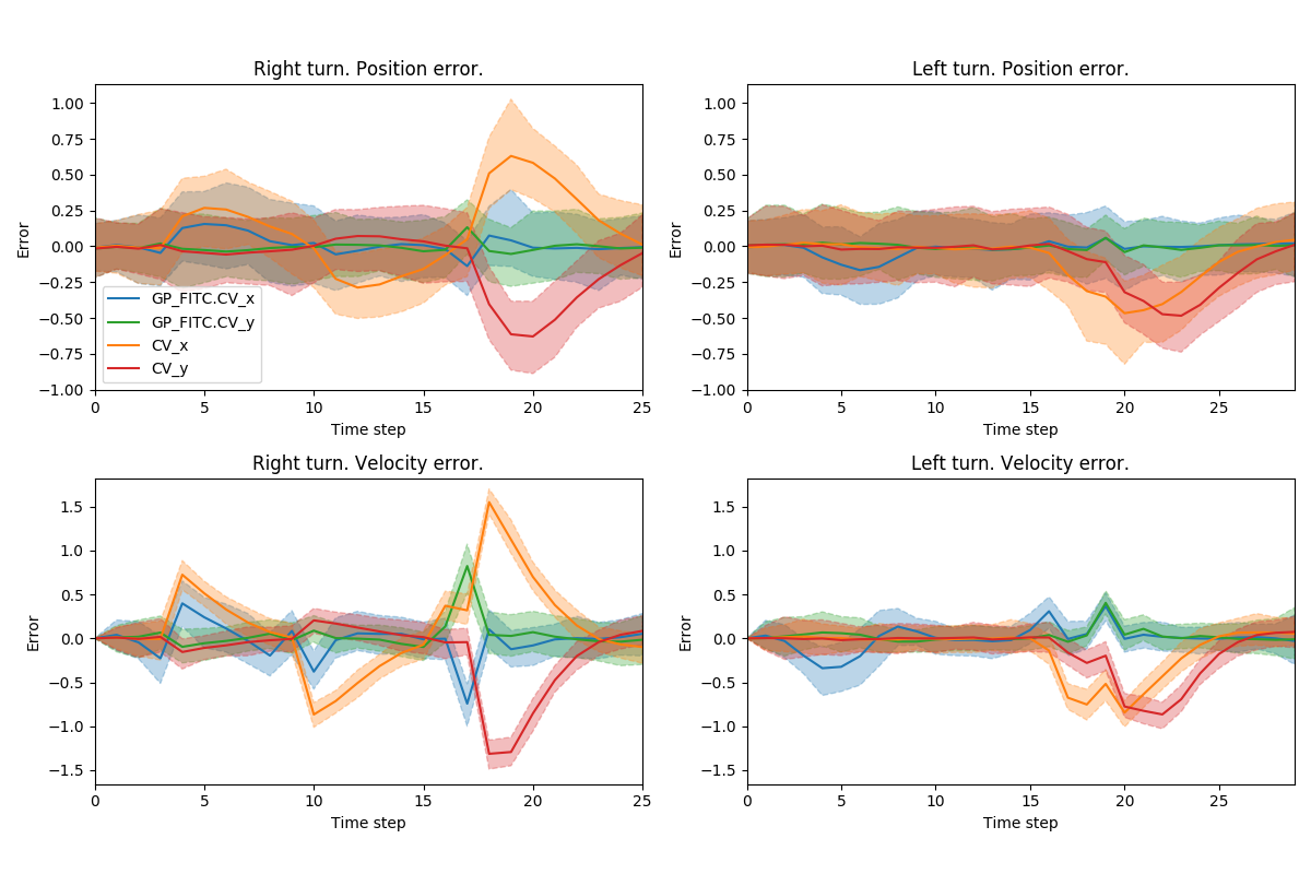
As a baseline, a cv model without the input learning was used. The Root Mean Squared Error (rmse) was calculated for each vehicle in each separate simulation and is visualized in Fig 4. Fig 4 visualizes trajectories of a cv, as well as of the gpassm where the input has been learned in advance using vehicles. The state errors for the first vehicle on each path are given in Fig 5LABEL:sub@fig:three-way-intersection:errors:iteration_0 and the last on each path in Fig 5LABEL:sub@fig:three-way-intersection:errors:iteration_-1. Note that this is not necessarily the first or last vehicle in total and also that there is no guarantee that the same number of vehicles have traversed each path.
From Fig 5LABEL:sub@fig:three-way-intersection:errors:iteration_0 it is evident that already for the first vehicle, there are benefits of including the gp. Before any accelerations are experienced, the model mimics the cv model exactly, but as accelerations come into play (around time step 3–4) the proposed model improves over the standard cv. This is due to the process noise being inherently nonwhite, which the gp captures. As the number of vehicles increases, see Fig 5LABEL:sub@fig:three-way-intersection:errors:iteration_-1, the gpassm learns the accelerations required to stay on the trajectory; see time step 15–25 for both paths. Lastly, even larger discrepancies between the gpassm and cv model would be evident if -step ahead prediction was used, since the cv would continue in a straight path and the gpassm would follow the average trajectory of the past vehicles.
Now, there are some peculiarities. For instance, see Fig 5LABEL:sub@fig:three-way-intersection:errors:iteration_-1 where the gpassm is actually worse than the cv model between time steps 3–10. This is caused by the acceleration discontinuity where the two paths split. This is also evident in Fig 2, (zoomed in area (b)), where the discontinuity causes a lot of small sideways accelerations where the gp is compensating for its own errors in a sense. Fig 2 also indicates that the learned acceleration mimic the true closely, see zoomed in area (a).
From Fig 4 it is evident that the gpassm follows the two paths better than the cv model. Whereas the cv model has a clear bias during the turns, the gpassm does not suffer from this.
V Conclusion and Future Work
A Gaussian Process Augmented State-Space Model has been proposed for learning unknown, but common, accelerations of vehicles through static environments. The model generalizes to cases where a simple motion model is sought after, but where the bias associated with such are not. The model was shown to improve over an ordinary Constant Velocity (cv) model and removed the bias when the accelerations were non-zero. An issue with the model is that it can not handle ambiguities in the input it is trying to learn and will in some of these cases perform worse than a cv model. The model is, however, attractive as it allows a simple motion model to be used in combination with a data-driven model for learning unknown characteristics of the underlying system online. It also facilitates distributed learning of unknown characteristics between systems that behave similarly. The learned input function itself might also be of use since its physical interpretation in many cases is easily found.
For the model to reach its full potential, the input ambiguities must be addressed. It is also necessary to find an efficient way to factorize the input space so as to reduce the computational burden, e.g., through dividing the area of interest into hexagonal surfaces [17]. Moreover, the approximation strategy of the Gaussian Process needs to be evaluated. If an inducing input approach is used, methods to add, remove, or move these online is necessary for reducing computational burden and to enable the model to be used in large-scale applications.
VI Acknowledgments
This work was partially supported by the Wallenberg AI, Autonomous Systems and Software Program (WASP) funded by the Knut and Alice Wallenberg Foundation.
Appendix A Derivation of model Jacobian
Given the model
| (A.1a) | ||||
| (A.1b) | ||||
| (A.1c) | ||||
the partial derivative of with respect to is given by
| (A.2) |
where the derivative of the squared exponential kernel is given by
| (A.3) |
and the derivative of the noise component is given by
| (A.4) |
For proof, see Appendix B in [8]. Now, (A.2) can be written
| (A.5) |
Furthermore the derivative of w.r.t. is given by
| (A.6) |
References
- [1] S. Särkkä, Bayesian Filtering and Smoothing. Cambridge University Press, 2010.
- [2] L. Ljung and T. Glad, Modeling and Identification of Dynamic Systems, 1st ed. Studentlitteratur, 2016.
- [3] A. Svensson, A. Solin, S. Särkkä, and T. B. Schön, “Computationally Efficient Bayesian Learning of Gaussian Process State Space Models,” in AISTATS 2016, Cadiz, Spain, may 2016, pp. 213–221.
- [4] A. Svensson and T. B. Schön, “A flexible state–space model for learning nonlinear dynamical systems,” Automatica, 2017.
- [5] R. Turner, M. P. Deisenroth, and C. E. Rasmussen, “State-space inference and learning with Gaussian processes,” J. Mach. Learn. Res., vol. 9, pp. 868–875, 2010.
- [6] R. Frigola, F. Lindsten, T. B. Schön, and C. E. Rasmussen, “Bayesian Inference and Learning in Gaussian Process State-Space Models with Particle MCMC,” Adv. Neural Inf. Process. Syst., pp. 1–9, 2013.
- [7] J. Ko and D. Fox, “GP-BayesFilters: Bayesian filtering using Gaussian process prediction and observation models,” Auton. Robots, vol. 27, no. 1, pp. 75–90, 2009.
- [8] C. Veibäck, J. Olofsson, T. R. Lauknes, and G. Hendeby, “Learning Target Dynamics While Tracking Using Gaussian Processes,” IEEE Trans. Aerosp. Electron. Syst., vol. 9251, pp. 1–10, 2019.
- [9] A. Svensson, T. B. Schön, A. Solin, and S. Särkkä, “Nonlinear State Space Model Identification Using a Regularized Basis Function Expansion,” in CAMSAP 2015, no. Ml, Cancun, Mexico, dec 2015, pp. 481–484.
- [10] J. Sjöberg, H. Hjalmarsson, and L. Ljung, “Neural Networks in System Identification,” IFAC Proc. Vol., vol. 27, no. 8, pp. 359–382, 1994.
- [11] R. Nayek, S. Chakraborty, and S. Narasimhan, “A Gaussian process latent force model for joint input-state estimation in linear structural systems,” Mech. Syst. Signal Process., vol. 128, pp. 497–530, 2019.
- [12] M. Ecker, N. Nieto, S. Käbitz, J. Schmalstieg, H. Blanke, A. Warnecke, and D. U. Sauer, “Calendar and cycle life study of Li(NiMnCo)O2-based 18650 lithium-ion batteries,” J. Power Sources, vol. 248, pp. 839–851, 2014.
- [13] X. R. Li and V. P. Jilkov, “Survey of Maneuvering Target Tracking. Part I: Dynamic Models,” IEEE Trans. Aerosp. Electron. Syst., vol. 39, no. 4, pp. 1333–1364, 2003.
- [14] C. E. Rasmussen and C. K. I. Williams, Gaussian Processes for Machine Learning. MIT Press, 2006.
- [15] J. Quiñonero-Candela and C. E. Rasmussen, “A Unifying View of Sparse Approximate Gaussian Process Regression,” J. Mach. Learn. Res., vol. 6, pp. 1939–1959, 2005.
- [16] A. Solin and S. Särkkä, “Hilbert space methods for reduced-rank Gaussian process regression,” Stat. Comput., vol. 30, no. 2, pp. 419–446, 2020.
- [17] M. Kok and A. Solin, “Scalable Magnetic Field SLAM in 3D Using Gaussian Process Maps,” in FUSION 2018, Cambridge, UK, jul 2018, pp. 1353–1360.
- [18] E. Snelson and Z. Ghahramani, “Sparse Gaussian Processes using Pseudo-inputs,” Adv. Neural Inf. Process. Syst. 18, pp. 1257–1264, 2006.
- [19] M. F. Huber, “Recursive Gaussian process: On-line regression and learning,” Pattern Recognit. Lett., vol. 45, no. 1, pp. 85–91, 2014.
- [20] M. K. Titsias, “Variational Learning of Inducing Variables in Sparse Gaussian Processes Michalis,” in AISTATS 2009, D. van Dyk and M. Welling, Eds., vol. 5. Clearwater, Florida: JMLR, apr 2009, pp. 567–574.