On the Performance of Cooperative NOMA Using MRC at Road Intersections in the Presence of Interference111Results related to this paper have been presented at the wireless and mobile computing, networking and communications (WiMob) 2019, Barcelona, Spain, October 2019 [1].

Baha Eddine Youcef Belmekki bahaeddine.belmekki@enseeiht.fr Abdelkrim  Hamza ahamza@usthb.dz Benoît Escrig benoit.escrig@enseeiht.fr University of Toulouse, IRIT/INP-ENSEEIHT Toulouse, BP 7122, 31071 Toulouse Cedex 7, France LISIC Laboratory, Electronic and Computer Faculty, USTHB, Algiers, Algeria
Abstract

As the traffic safety has become of utmost importance, much attention is given to intelligent transportation systems (ITSs), and more particularly to vehicular communications (VCs). Moreover, 50 % of all crashes happen at road intersections, which makes theme a critical areas. In this paper, we investigate the improvement when implementing maximum ratio combining (MRC) in cooperative VCs transmission schemes using non-orthogonal multiple access scheme (NOMA) at road intersections. We consider that a source transmits a message to two destinations with a aid of a relay. The transmission undergoes interference generated from a set of vehicles on the roads. We obtained closed form outage probability expressions, and we extend the derivation for a scenario involving K𝐾K destination nodes and several road lanes. The performance of MRC cooperative NOMA is compared with the standard cooperative NOMA, and we show that implementing MRC with NOMA offers a significant improvement over the standard cooperative NOMA. Also, we compare the performance of MRC using NOMA with MRC cooperative orthogonal multiple access (OMA), and demonstrate that NOMA significantly outperforms OMA. We conclude that it is always beneficial to use MRC and NOMA even at the cost of implementation complexity. Finally, we demonstrate that the outage probability increases drasticallyen the vehicles are closer to the road intersection, and that using MRC with NOMA improves significantly the performance in this context. To verify the correctness of our analysis, extensive Monte-Carlo simulations are carried out.

keywords:
5G, NOMA, interference, outage probability, cooperative, MRC, intersections.
journal: Journal of  Templatesjournal: Arxiv

1 Introduction

1.1 Motivation

As the traffic safety has become of utmost importance, much attention is given to intelligent transportation systems (ITSs), and more specifically to vehicular communications (VCs) [2, 3]. VCs offer a wide range of applications such as, traffic state, autonomous driving, and safety [4, 5, 6]. According to World Health organization, over 1.25 million people die each year on the roads, and road traffic crashes are the number one cause of death among young people [7]. Moreover, 50 % of all crashes are in junction areas (intersections) including fatal crashes, injury crashes and property damage crashes [8]. This makes intersections critical areas not only for vehicles, but also for pedestrians and cyclists. VCs have numerous applications to prevent accidents, or alert vehicles when accidents happen in their surroundings. Thus, low latency and high reliability communications are mandatory in safety-based VCs. To increase spectral efficiency and data rate [9] in the fifth generation (5G) of wireless communication systems, non-orthogonal multiple access (NOMA) is an promising candidate as a multiple access scheme. NOMA, unlike orthogonal multiple access (OMA), allows several users to use the same resource with several power allocation levels. Also, cooperative transmissions have been show to increase the reliability of the transmission link [10, 11, 12]. On the other hand, co-channel interference is one of the major impairments that can degrade a transmission in VCs [13, 14, 15]. Hence, in this paper we propose to study the impact of interference in cooperative VCs at intersections using NOMA.

1.2 Related Works

1.2.1 NOMA Works

The performance of NOMA has been well studied in the literature (see [16, 17, 18] and the references therein). As far as the impact of interference on NOMA is concerned, several papers have studied its effect [19]. The authors in [20] analysed the impact of interference on a NOMA uplink transmission. The authors also analyzed the performance of a NOMA downlink transmission with a selection based pairing in [21]. The improvement of using cooperative transmissions in NOMA have been also well investigated [22, 23, 24, 18]. A scenario involving M𝑀M number of randomly deployed users was investigated in [18]. The authors also evaluated the ergodic rate and outage performance in [24]. In [22], the authors studied the impact of relay selection on cooperative NOMA, and showed that the two-stage scheme can achieve the optimal diversity gain and the minimal outage probability. However, the impact of implementing NOMA into VCs has been lacking in the literature.

1.2.2 VCs Works

The performance of VCs in the presence of interference has attracted a lot of attention [25, 26, 27]. Mainly, there are two types of scenarios in VCs, highways scenarios and intersections scenarios. Considering highway scenarios, the authors in [26] investigated the performance of RTS/CTS protocol considering Nakagami-m𝑚m channels fading. In [25], the authors studied how the interference affects the safety of vehicles in a VCs. The authors also derived the packet success probability for two different traffic models in VCs [28]. The authors in [27] investigated the performance of carrier sense multiple access (CSMA) protocols, and derived the expressions of packet success probability. In [29], the authors derived the outage probability and rate coverage probability when a line of sight path to the base station is absent.

Considering intersection scenarios, a success probability expression of a simple intersection scenario was derived in [30]. The authors in [31] extended the work of [30] and derived the success probability considering limited road segments with different path loss models. The authors of [31] also studied the average and the fine-grained reliability in an interference-limited vehicle to vehicle (V2V) communications with the aid of the meta distribution in [32]. The authors [33] in investigated the performance of V2V communications for orthogonal streets. The authors also studied V2V communications at intersections and showed that, the performance of the ALOHA protocol can be considered as lower bound of performance of the CSMA protocols [34]. The effect of vehicles mobility and interference dependence has been investigated in [35]. The authors also, studied the performance of three transmission schemes at intersection in line of sight scenario and non light of sight scenario considering Nakagami-m𝑚m fading channels in [36, 37].

However, the performance of NOMA in VCs is lacking in the literature. The first to tackle this issue are the authors of the paper at hand. They computed the outage probability and average achievable rate of NOMA at intersection roads considering direct transmissions [38, 39] and cooperative transmissions [40, 41]. They also investigated the performance of NOMA in millimeter wave vehicular communications in [42, 43]. In [44], the authors proposed an adaptive NOMA protocol in VCs.

In this paper, the authors study the feasibility and improvement in performance by implementing both NOMA and maximum ratio combining (MRC) in VCs. Hence, we compare the proposed scheme with the classical OMA, and the classical cooperative NOMA, and see if the improvements justify and outweigh the complexity of implementing MRC and NOMA in VCs.

1.3 Contributions

The contributions of this paper are as follows:

  • 1.

    We establish a framework for performance analysis of VCs under Rayleigh fading and two perpendicular roads containing one-dimensional Poisson field of interference. We analyze the performance of implementing MRC in cooperative VCs transmission schemes using NOMA at intersections in terms of outage probability. We obtained closed form outage probability expressions. We further extend the derivations when K𝐾K destination nodes are involved, and to a realistic intersection scenario involving multiple lanes.

  • 2.

    We compare the performance of MRC cooperative NOMA with a classical cooperative NOMA [41], and show that implementing MRC in cooperative NOMA transmission offers a significant improvement over the classical cooperative NOMA in terms of outage probability. We also compare the performance of MRC cooperative NOMA with MRC cooperative OMA [35], and show that NOMA offers a better performance than OMA. It is shown that the outage probability increases when the vehicles are closer to the road intersection, and that using MRC considering NOMA improves significantly the performance in this context.

  • 3.

    The relationships between system performance and different network parameters such as NOMA power allocation coefficient, date rates, channel access probability, intensity of potential interfering vehicles, relay position, noise power levels, successive interference cancellation (SIC) coefficient are discussed. The results clearly demonstrate the advantages of implementing MRC into NOMA the performance in VCs, even at the cost of implementation complexity.

  • 4.

    We show that as we increases the data rate of D2subscript𝐷2D_{2}, MRC transmission using NOMA offers a better performance than MRC transmission using OMA. Whereas for D1subscript𝐷1D_{1}, low data rates are suitable, since there is a condition imposed to its data rate. We also show how the imperfect SIC process can degrade the performance of NOMA. We also show that MRC transmission using NOMA outperforms cooperative NOMA. Finally, we investigate the best relay position, and show that the optimal relay position for D1subscript𝐷1D_{1} and D2subscript𝐷2D_{2} is near the destination nodes.

  • 5.

    To confirm the correctness of our theoretical derivations, extensive Monte-Carlo simulations are carried out.

1.4 Organization

The rest of this paper is organized as follows. Section 2 presents the system model. In Section 3, outage analytical expressions are derived. The Laplace transform expressions are presented in Section 4. Extension to multiple lanes scenario is investigated in Section 5. Simulations and discussions are in Section 6. Finally, we conclude the paper in Section 7.

2 System Model
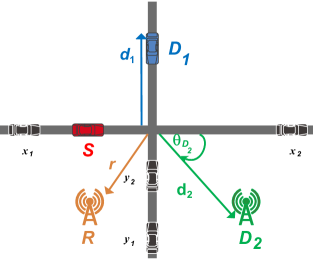
Refer to caption
Figure 1: Cooperative NOMA system model for vehicular communications involving two destination nodes and a relay node. For this example, S𝑆S is a vehicle, R𝑅R is an infrastructure, D1subscript𝐷1D_{1} is a vehicle, and D2subscript𝐷2D_{2} is an infrastructure.

2.1 Intersection Scenario

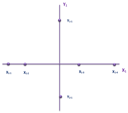
We consider a cooperative transmission using NOMA between a source S𝑆S and two destinations D1subscript𝐷1D_{1} and D2subscript𝐷2D_{2}, with the aid of a relay R𝑅R as shown in Fig.1. As both V2V and V2I communications are of interest222The Doppler shift and time-varying effect of V2V and V2I channels is beyond the scope of this paper., the nodes S𝑆S,R𝑅R, D1subscript𝐷1D_{1} and D2subscript𝐷2D_{2} can be on the roads (as vehicles), or outside the roads (as infrastructures). For instance in Fig.1, the configuration is as follows: S𝑆S and D1subscript𝐷1D_{1} are vehicles, whereas R𝑅R and D2subscript𝐷2D_{2} are infrastructures. For the sake of notation simplicity, we denote by M𝑀M the receiving node, and by m𝑚m the distance between the node M𝑀M and the intersection, where M{R,D1,D2}𝑀𝑅subscript𝐷1subscript𝐷2M\in\{R,D_{1},D_{2}\} and m{r,d1,d2}𝑚𝑟subscript𝑑1subscript𝑑2m\in\{r,d_{1},d_{2}\}, as shown in Fig.1. Also, the term θMsubscript𝜃𝑀\theta_{M} denotes the angle between the node M𝑀M and the X𝑋X road.

In this paper, we study the performance at an intersection. The intersection has two two perpendicular roads, an horizontal road denoted by X𝑋X, and a vertical road denoted by Y𝑌Y. We extend the analysis to the case when the intersection involves multiple lanes in Section 5.

The set of nodes {S,R,D1,D2}𝑆𝑅subscript𝐷1subscript𝐷2\{{S,R,D_{1},D_{2}}\} is subject to interference originated from transmitting vehicles located on the roads. The set of interfering vehicles located on the Z𝑍Z road where Z{X,Y}𝑍𝑋𝑌Z\in\{X,Y\}, denoted by ΦZsubscriptΦ𝑍\Phi_{Z} are modeled as a one-dimensional homogeneous Poisson point process (1D-HPPP), that is, ΦZ1D-HPPP(λZ,z)similar-tosubscriptΦ𝑍1D-HPPPsubscript𝜆𝑍𝑧\Phi_{Z}\sim\textrm{1D-HPPP}(\lambda_{Z},z), where z{x,y}𝑧𝑥𝑦z\in\{x,y\} and λZsubscript𝜆𝑍\lambda_{Z} are the position of interfering vehicles and their intensity on the Z𝑍Z road, respectively. This implies that the number of potential interfering vehicles within any closed and bounded set \mathcal{B}\subseteq\mathbb{R} is a Poisson random variable with parameter λ||𝜆\lambda|\mathcal{B}|.

S𝑆SR𝑅RD1subscript𝐷1D_{1}D2subscript𝐷2D_{2} First phase           S𝑆SR𝑅RD1subscript𝐷1D_{1}D2subscript𝐷2D_{2} Second phase

Figure 2: Transmission scheme using MRC and NOMA.

2.2 MRC and Cooperative Protocol

In this paper, we use Decode and Forward (DF) cooperative protocol [45, 46]. The transmission occurs in two phases, the duration of each phase is one time slot. Finally we consider we use MRC in NOMA setup as shown in Fig.2. In the first phase, S𝑆S broadcasts the message, and the nodes R𝑅R, D1subscript𝐷1D_{1} and D2subscript𝐷2D_{2} try to decode the message. In the second phase, if R𝑅R decodes S𝑆S message, it broadcasts the message to D1subscript𝐷1D_{1} and D2subscript𝐷2D_{2}. Then, D1subscript𝐷1D_{1} and D2subscript𝐷2D_{2} add the power received in the first phase from S𝑆S and (if R𝑅R decodes S𝑆S message) the power received from R𝑅R during the second phase to decode the message.

2.3 NOMA Scenario and Assumptions

In NOMA, there are two main ways to order the users. The first one is to order the nodes according to their channel stats. Hence, the user with the weakest channel state comes first in the decoding order (see [18, 47] and references therein). The second one is that, the users are sorted according to their quality of service (QoS) priorities. Hence, a user with the higher priority comes first in the seconding order. It has been show in [22, 48], that ordering users according to their QoS is more realistic and reasonable assumption, since in practice, it is very likely that users who want to participate in NOMA have similar channel conditions. Without loss of generality, we study the case in which node D1subscript𝐷1D_{1} has to be served immediately with a low data rate. For example, D1subscript𝐷1D_{1} can be a vehicle that needs to receive safety information containing a few bytes, such as a road flood warning or incident avoidance alert message. Whereas node D2subscript𝐷2D_{2} requires relatively high data rate but can be served later. For instance D2subscript𝐷2D_{2} can be a user that accesses the internet connection.

2.4 Channel Model

We consider slotted ALOHA protocol with parameter p𝑝p, i.e., every node can access the medium with a probability p𝑝p. This performs an independent thinning the parent 1D-HPPP by probability p𝑝p. Hence, the set of interfering vehicles at a given time slot also follow a a 1D-HPPP with intensity pλ𝑝𝜆p\lambda.

The transmission between a node a𝑎a and b𝑏b experience a path loss given by lab=(Arab)αsubscript𝑙𝑎𝑏superscript𝐴subscript𝑟𝑎𝑏𝛼l_{ab}=(Ar_{ab})^{-\alpha} , where A𝐴A is a constant depending on the antenna characteristics, rab=absubscript𝑟𝑎𝑏norm𝑎𝑏r_{ab}=\|a-b\|, and α𝛼\alpha is the path loss exponent. All the node transmit with power P𝑃P.

The signal transmitted by S𝑆S, denoted χSsubscript𝜒𝑆\chi_{S} is a mixture of the message intended to D1subscript𝐷1D_{1} and D2subscript𝐷2D_{2}. This can be expressed as

χS=a1χD1+a2χD2,subscript𝜒𝑆subscript𝑎1subscript𝜒𝐷1subscript𝑎2subscript𝜒𝐷2\chi_{S}=\sqrt{a_{1}}\chi_{D1}+\sqrt{a_{2}}\chi_{D2},

where aisubscript𝑎𝑖a_{i} is the power coefficients allocated to Disubscript𝐷𝑖D_{i}, and χDisubscript𝜒𝐷𝑖\chi_{Di} is the message intended to Disubscript𝐷𝑖D_{i}, where i{1,2}𝑖12i\in\{1,2\}. Since D1subscript𝐷1D_{1} has higher power than D2subscript𝐷2D_{2}, that is a1a2subscript𝑎1subscript𝑎2a_{1}\geq a_{2}, then D1subscript𝐷1D_{1} comes first in the decoding order. Note that, a1+a2=1subscript𝑎1subscript𝑎21a_{1}+a_{2}=1.
The signal received at R𝑅R and Disubscript𝐷𝑖D_{i}, denoted respectively by 𝒴Rsubscript𝒴𝑅\mathcal{Y}_{R} and 𝒴Disubscript𝒴subscript𝐷𝑖\mathcal{Y}_{D_{i}}, during the first time slot are expressed as

𝒴R=hSRPlSRχSThe signal of interest that contains D1 message and D2 message+subscript𝒴𝑅limit-fromsubscriptsubscript𝑆𝑅𝑃subscript𝑙𝑆𝑅subscript𝜒𝑆The signal of interest that contains D1 message and D2 message\displaystyle\mathcal{Y}_{R}=\underbrace{h_{SR}\sqrt{Pl_{SR}}\>\chi_{S}}_{\text{The signal of interest that contains $D_{1}$ message and $D_{2}$ message}}+
xΦXRhRxPlRxχxAggregate interference form the Y road at R+yΦYRhRyPlRyχyAggregate interference form the Y road at R+σ2Noise related term,subscriptsubscript𝑥subscriptΦsubscript𝑋𝑅subscript𝑅𝑥𝑃subscript𝑙𝑅𝑥subscript𝜒𝑥Aggregate interference form the Y road at Rsubscriptsubscript𝑦subscriptΦsubscript𝑌𝑅subscript𝑅𝑦𝑃subscript𝑙𝑅𝑦subscript𝜒𝑦Aggregate interference form the Y road at Rsubscriptsuperscript𝜎2Noise related term\displaystyle\underbrace{\sum_{x\in\Phi_{X_{R}}}h_{Rx}\sqrt{Pl_{Rx}}\>\chi_{x}}_{\text{Aggregate interference form the $Y$ road at $R$}}+\underbrace{\sum_{y\in\Phi_{Y_{R}}}h_{Ry}\sqrt{Pl_{Ry}}\>\chi_{y}}_{\text{Aggregate interference form the $Y$ road at $R$}}+\underbrace{\sigma^{2}}_{\text{Noise related term}},

and

𝒴Di=hSDiPlSDiχS+subscript𝒴subscript𝐷𝑖limit-fromsubscript𝑆subscript𝐷𝑖𝑃subscript𝑙𝑆subscript𝐷𝑖subscript𝜒𝑆\displaystyle\mathcal{Y}_{D_{i}}=h_{SD_{i}}\sqrt{Pl_{SD_{i}}}\>\chi_{S}+
xΦXDihDixPlDixχxAggregate interference form the X road at Di+yΦYDihDiyPlDiyχyAggregate interference form the Y road at Di+σ2.subscriptsubscript𝑥subscriptΦsubscript𝑋subscript𝐷𝑖subscriptsubscript𝐷𝑖𝑥𝑃subscript𝑙subscript𝐷𝑖𝑥subscript𝜒𝑥Aggregate interference form the X road at Disubscriptsubscript𝑦subscriptΦsubscript𝑌subscript𝐷𝑖subscriptsubscript𝐷𝑖𝑦𝑃subscript𝑙subscript𝐷𝑖𝑦subscript𝜒𝑦Aggregate interference form the Y road at Disuperscript𝜎2\displaystyle\underbrace{\sum_{x\in\Phi_{X_{D_{i}}}}h_{D_{i}x}\sqrt{Pl_{D_{i}x}}\>\chi_{x}}_{\text{Aggregate interference form the $X$ road at $D_{i}$}}+\underbrace{\sum_{y\in\Phi_{Y_{D_{i}}}}h_{D_{i}y}\sqrt{Pl_{D_{i}y}}\>\chi_{y}}_{\text{Aggregate interference form the $Y$ road at $D_{i}$}}+\sigma^{2}.

The signal received at Disubscript𝐷𝑖D_{i}, denoted by 𝒴Disubscript𝒴subscript𝐷𝑖\mathcal{Y}_{D_{i}}, during the second time slot is expressed as

𝒴Di=hRDiPlRDiχR+subscript𝒴subscript𝐷𝑖limit-fromsubscript𝑅subscript𝐷𝑖𝑃subscript𝑙𝑅subscript𝐷𝑖subscript𝜒𝑅\displaystyle\mathcal{Y}_{D_{i}}=h_{RD_{i}}\sqrt{Pl_{RD_{i}}}\>\chi_{R}+
xΦXDihDixPlDixχxAggregate interference form the Y road at Di+yΦYDihDiyPlDiyχyAggregate interference form the Y road at Di+σ2,subscriptsubscript𝑥subscriptΦsubscript𝑋subscript𝐷𝑖subscriptsubscript𝐷𝑖𝑥𝑃subscript𝑙subscript𝐷𝑖𝑥subscript𝜒𝑥Aggregate interference form the Y road at Disubscriptsubscript𝑦subscriptΦsubscript𝑌subscript𝐷𝑖subscriptsubscript𝐷𝑖𝑦𝑃subscript𝑙subscript𝐷𝑖𝑦subscript𝜒𝑦Aggregate interference form the Y road at Disuperscript𝜎2\displaystyle\underbrace{\sum_{x\in\Phi_{X_{D_{i}}}}h_{D_{i}x}\sqrt{Pl_{D_{i}x}}\>\chi_{x}}_{\text{Aggregate interference form the $Y$ road at $D_{i}$}}+\underbrace{\sum_{y\in\Phi_{Y_{D_{i}}}}h_{D_{i}y}\sqrt{Pl_{D_{i}y}}\>\chi_{y}}_{\text{Aggregate interference form the $Y$ road at $D_{i}$}}+\sigma^{2},

where signals transmitted by the interfering vehicles x𝑥x and y𝑦y, are denoted by χxsubscript𝜒𝑥\chi_{x} and χysubscript𝜒𝑦\chi_{y}, respectively. The term habsubscript𝑎𝑏h_{ab} denotes the fading coefficient between node a𝑎a and b𝑏b, and it is modeled as 𝒞𝒩(0,1)𝒞𝒩01\mathcal{CN}(0,1) [49, 50, 51], hence |hab|2exp(1)similar-tosuperscriptsubscript𝑎𝑏21|h_{ab}|^{2}\sim\exp(1). The aggregate interference is defined as

IZM=zΦZMP|hMz|2lMz,subscript𝐼subscript𝑍𝑀subscript𝑧subscriptΦsubscript𝑍𝑀𝑃superscriptsubscript𝑀𝑧2subscript𝑙𝑀𝑧I_{Z_{M}}=\sum_{z\in\Phi_{Z_{M}}}P|h_{Mz}|^{2}l_{Mz}, (1)

where IZMsubscript𝐼subscript𝑍𝑀I_{Z_{M}} denotes the aggregate interference from the Z𝑍Z road at M𝑀M, ΦZMsubscriptΦsubscript𝑍𝑀\Phi_{Z_{M}} denotes the set of the interfering vehicles from the Z𝑍Z road at M𝑀M.

3 Outage Analytical Derivations

3.1 Outage Events

We define an outage event at the receiving node when the signal-to-interference plus noise ratio (SINR) at the receiver is below a given threshold. According to SIC [52], D1subscript𝐷1D_{1} is decoded first since it has the higher power allocation, and D2subscript𝐷2D_{2} message is considered as interference. The outage event at R𝑅R to not decode D1subscript𝐷1D_{1}, denoted 𝒜R1(Θ1)subscript𝒜subscript𝑅1subscriptΘ1\mathcal{A}_{R_{1}}(\Theta_{1}), is defined as

𝒜R1(Θ1)P|hSR|2lSRa1P|hSR|2lSRa2+IXR+IYR+σ2<Θ1,subscript𝒜subscript𝑅1subscriptΘ1𝑃superscriptsubscript𝑆𝑅2subscript𝑙𝑆𝑅subscript𝑎1𝑃superscriptsubscript𝑆𝑅2subscript𝑙𝑆𝑅subscript𝑎2subscript𝐼subscript𝑋𝑅subscript𝐼subscript𝑌𝑅superscript𝜎2subscriptΘ1\mathcal{A}_{R_{1}}(\Theta_{1})\triangleq\frac{P|h_{SR}|^{2}l_{SR}\,a_{1}}{P|h_{SR}|^{2}l_{SR}a_{2}+I_{X_{R}}+I_{Y_{R}}+\sigma^{2}}<\Theta_{1}, (2)

where Θ1=2211subscriptΘ1superscript22subscript11\Theta_{1}=2^{2\mathcal{R}_{1}}-1, and 1subscript1\mathcal{R}_{1} is the target data rate of D1subscript𝐷1D_{1}.

Since D2subscript𝐷2D_{2} has a lower power allocation, R𝑅R has to decode D1subscript𝐷1D_{1} message, then decode D2subscript𝐷2D_{2} message. The outage event at R𝑅R to not decode D2subscript𝐷2D_{2} message, denoted 𝒜R2(Θ2)subscript𝒜subscript𝑅2subscriptΘ2\mathcal{A}_{R_{2}}(\Theta_{2}), is defined as

𝒜R2(Θ2)P|hSR|2lSRa2βP|hSR|2lSRa1+IXR+IYR+σ2<Θ2,subscript𝒜subscript𝑅2subscriptΘ2𝑃superscriptsubscript𝑆𝑅2subscript𝑙𝑆𝑅subscript𝑎2𝛽𝑃superscriptsubscript𝑆𝑅2subscript𝑙𝑆𝑅subscript𝑎1subscript𝐼subscript𝑋𝑅subscript𝐼subscript𝑌𝑅superscript𝜎2subscriptΘ2\mathcal{A}_{R_{2}}(\Theta_{2})\triangleq\frac{P|h_{SR}|^{2}l_{SR}\,a_{2}}{\beta P|h_{SR}|^{2}l_{SR}\,a_{1}+I_{X_{R}}+I_{Y_{R}}+\sigma^{2}}<\Theta_{2}, (3)

where Θ2=2221subscriptΘ2superscript22subscript21\Theta_{2}=2^{2\mathcal{R}_{2}}-1, and 2subscript2\mathcal{R}_{2} is the target data rate of D2subscript𝐷2D_{2}.

Similarly, the outage event at D1subscript𝐷1D_{1} to not decode its intended message in the first phase (SD1𝑆subscript𝐷1S\rightarrow D_{1}), denoted D11(Θ1)subscriptsubscript𝐷11subscriptΘ1\mathcal{B}_{D_{1\rightarrow 1}}(\Theta_{1}), is given by

D11(Θ1)P|hSD1|2lSD1a1P|hSD1|2lSD1a2+IXD1+IYD1+σ2<Θ1.subscriptsubscript𝐷11subscriptΘ1𝑃superscriptsubscript𝑆subscript𝐷12subscript𝑙𝑆subscript𝐷1subscript𝑎1𝑃superscriptsubscript𝑆subscript𝐷12subscript𝑙𝑆subscript𝐷1subscript𝑎2subscript𝐼subscript𝑋subscript𝐷1subscript𝐼subscript𝑌subscript𝐷1superscript𝜎2subscriptΘ1\mathcal{B}_{D_{1\rightarrow 1}}(\Theta_{1})\triangleq\frac{P|h_{SD_{1}}|^{2}l_{SD_{1}}\,a_{1}}{P|h_{SD_{1}}|^{2}l_{SD_{1}}a_{2}+I_{X_{D_{1}}}+I_{Y_{D_{1}}}+\sigma^{2}}<\Theta_{1}. (4)

Finally, in order for D2subscript𝐷2D_{2} to decode its intended message, it has to decode D1subscript𝐷1D_{1} message. The outage event at D2subscript𝐷2D_{2} to not decode D1subscript𝐷1D_{1} message in the first phase (SD2𝑆subscript𝐷2S\rightarrow D_{2}), denoted D21(Θ1)subscriptsubscript𝐷21subscriptΘ1\mathcal{B}_{D_{2\rightarrow 1}}(\Theta_{1}), and the outage event at D2subscript𝐷2D_{2} to not decode its intended message, denoted D22(Θ2)subscriptsubscript𝐷22subscriptΘ2\mathcal{B}_{D_{2\rightarrow 2}}(\Theta_{2}), are respectively given by

D21(Θ1)P|hSD2|2lSD2a1P|hSD2|2lSD2a2+IXD2+IYD2+σ2<Θ1,subscriptsubscript𝐷21subscriptΘ1𝑃superscriptsubscript𝑆subscript𝐷22subscript𝑙𝑆subscript𝐷2subscript𝑎1𝑃superscriptsubscript𝑆subscript𝐷22subscript𝑙𝑆subscript𝐷2subscript𝑎2subscript𝐼subscript𝑋subscript𝐷2subscript𝐼subscript𝑌subscript𝐷2superscript𝜎2subscriptΘ1\mathcal{B}_{D_{2\rightarrow 1}}(\Theta_{1})\triangleq\frac{P|h_{SD_{2}}|^{2}l_{SD_{2}}\,a_{1}}{P|h_{SD_{2}}|^{2}l_{SD_{2}}a_{2}+I_{X_{D_{2}}}+I_{Y_{D_{2}}}+\sigma^{2}}<\Theta_{1}, (5)

and

D22(Θ2)P|hSD2|2lSD2a2βP|hSD2|2lSD2a1+IXD2+IYD2+σ2<Θ2.subscriptsubscript𝐷22subscriptΘ2𝑃superscriptsubscript𝑆subscript𝐷22subscript𝑙𝑆subscript𝐷2subscript𝑎2𝛽𝑃superscriptsubscript𝑆subscript𝐷22subscript𝑙𝑆subscript𝐷2subscript𝑎1subscript𝐼subscript𝑋subscript𝐷2subscript𝐼subscript𝑌subscript𝐷2superscript𝜎2subscriptΘ2\mathcal{B}_{D_{2\rightarrow 2}}(\Theta_{2})\triangleq\frac{P|h_{SD_{2}}|^{2}l_{SD_{2}}\,a_{2}}{\beta P|h_{SD_{2}}|^{2}l_{SD_{2}}\,a_{1}+I_{X_{D_{2}}}+I_{Y_{D_{2}}}+\sigma^{2}}<\Theta_{2}. (6)

During the second phase, D1subscript𝐷1D_{1} adds the power received from S𝑆S and from R𝑅R. Hence, the outage event at D1subscript𝐷1D_{1} to not decode its message in the second phase, denoted 𝒞D11(Θ1)subscript𝒞subscript𝐷11subscriptΘ1\mathcal{C}_{D_{1\rightarrow 1}}(\Theta_{1}), is expressed as

𝒞D11(Θ1)P[SD1,RD1](|h|2,l)a1P[SD1,RD1](|h|2,l)a2+IXD1+IYD1+σ2<Θ1,subscript𝒞subscript𝐷11subscriptΘ1𝑃subscript𝑆subscript𝐷1𝑅subscript𝐷1superscript2𝑙subscript𝑎1𝑃subscript𝑆subscript𝐷1𝑅subscript𝐷1superscript2𝑙subscript𝑎2subscript𝐼subscript𝑋subscript𝐷1subscript𝐼subscript𝑌subscript𝐷1superscript𝜎2subscriptΘ1\mathcal{C}_{D_{1\rightarrow 1}}(\Theta_{1})\triangleq\frac{P\sum_{[SD_{1},RD_{1}]}(|h|^{2},l)\,a_{1}}{P\sum_{[SD_{1},RD_{1}]}(|h|^{2},l)\,a_{2}+I_{X_{D_{1}}}+I_{Y_{D_{1}}}+\sigma^{2}}<\Theta_{1}, (7)

where

[SDi,RDi](|h|2,l)=|hSDi|2lSDi+|hRDi|2lRD2.subscript𝑆subscript𝐷𝑖𝑅subscript𝐷𝑖superscript2𝑙superscriptsubscript𝑆subscript𝐷𝑖2subscript𝑙𝑆subscript𝐷𝑖superscriptsubscript𝑅subscript𝐷𝑖2subscript𝑙𝑅subscript𝐷2\sum_{[SD_{i},RD_{i}]}(|h|^{2},l)=|h_{SD_{i}}|^{2}l_{SD_{i}}+|h_{RD_{i}}|^{2}l_{RD_{2}}.

In the same way, in the second phase, D2subscript𝐷2D_{2} adds the power received from S𝑆S and from R𝑅R. Hence, the outage event at D2subscript𝐷2D_{2} to not decode D1subscript𝐷1D_{1} message, denoted 𝒞D21(Θ1)subscript𝒞subscript𝐷21subscriptΘ1\mathcal{C}_{D_{2\rightarrow 1}}(\Theta_{1}), and the outage event at D2subscript𝐷2D_{2} to not decode its message, denoted 𝒞D22(Θ2)subscript𝒞subscript𝐷22subscriptΘ2\mathcal{C}_{D_{2\rightarrow 2}}(\Theta_{2}), are respectively expressed as

𝒞D21(Θ1)P[SD2,RD2](|h|2,l)a1P[SD2,RD2](|h|2,l)a2+IXD2+IYD2+σ2<Θ1,subscript𝒞subscript𝐷21subscriptΘ1𝑃subscript𝑆subscript𝐷2𝑅subscript𝐷2superscript2𝑙subscript𝑎1𝑃subscript𝑆subscript𝐷2𝑅subscript𝐷2superscript2𝑙subscript𝑎2subscript𝐼subscript𝑋subscript𝐷2subscript𝐼subscript𝑌subscript𝐷2superscript𝜎2subscriptΘ1\mathcal{C}_{D_{2\rightarrow 1}}(\Theta_{1})\triangleq\frac{P\sum_{[SD_{2},RD_{2}]}(|h|^{2},l)\,a_{1}}{P\sum_{[SD_{2},RD_{2}]}(|h|^{2},l)\,a_{2}+I_{X_{D_{2}}}+I_{Y_{D_{2}}}+\sigma^{2}}<\Theta_{1}, (8)

and

𝒞D22(Θ2)P[SD2,RD2](|h|2,l)a2βP[SD2,RD2](|h|2,l)a1+IXD2+IYD2+σ2<Θ2.subscript𝒞subscript𝐷22subscriptΘ2𝑃subscript𝑆subscript𝐷2𝑅subscript𝐷2superscript2𝑙subscript𝑎2𝛽𝑃subscript𝑆subscript𝐷2𝑅subscript𝐷2superscript2𝑙subscript𝑎1subscript𝐼subscript𝑋subscript𝐷2subscript𝐼subscript𝑌subscript𝐷2superscript𝜎2subscriptΘ2\mathcal{C}_{D_{2\rightarrow 2}}(\Theta_{2})\triangleq\frac{P\sum_{[SD_{2},RD_{2}]}(|h|^{2},l)\,a_{2}}{\beta P\sum_{[SD_{2},RD_{2}]}(|h|^{2},l)\,a_{1}+I_{X_{D_{2}}}+I_{Y_{D_{2}}}+\sigma^{2}}<\Theta_{2}. (9)

The overall outage event related to D1subscript𝐷1D_{1}, denoted O(1)subscriptO1\textit{O}_{(1)}, is given by

O(1)[D11(Θ1)𝒜R1(Θ1)][𝒜R1C(Θ1)𝒞D11(Θ1)].subscriptO1delimited-[]subscriptsubscript𝐷11subscriptΘ1subscript𝒜subscript𝑅1subscriptΘ1delimited-[]superscriptsubscript𝒜subscript𝑅1𝐶subscriptΘ1subscript𝒞subscript𝐷11subscriptΘ1\textit{O}_{(1)}\triangleq\Big{[}\mathcal{B}_{D_{1\rightarrow 1}}(\Theta_{1})\cap\mathcal{A}_{R_{1}}(\Theta_{1})\Big{]}\cup\Big{[}\mathcal{A}_{R_{1}}^{C}(\Theta_{1})\cap\mathcal{C}_{D_{1\rightarrow 1}}(\Theta_{1})\Big{]}. (10)

Finally, the overall outage event related to D2subscript𝐷2D_{2}, denoted O(2)subscriptO2\textit{O}_{(2)}, is given by

O(2)subscriptO2absent\displaystyle\textit{O}_{(2)}\triangleq [{i=12D2i(Θi)}{i=12𝒜Ri(Θi)}]delimited-[]superscriptsubscript𝑖12subscriptsubscript𝐷2𝑖subscriptΘ𝑖superscriptsubscript𝑖12subscript𝒜subscript𝑅𝑖subscriptΘ𝑖\displaystyle\left[\Bigg{\{}\bigcup_{i=1}^{2}\mathcal{B}_{D_{2\rightarrow i}}(\Theta_{i})\Bigg{\}}\cap\Bigg{\{}\bigcup_{i=1}^{2}\mathcal{A}_{R_{i}}(\Theta_{i})\Bigg{\}}\right]
[{i=12𝒜RiC(Θi)}{i=12𝒞D2i(Θi)}].delimited-[]superscriptsubscript𝑖12superscriptsubscript𝒜subscript𝑅𝑖𝐶subscriptΘ𝑖superscriptsubscript𝑖12subscript𝒞subscript𝐷2𝑖subscriptΘ𝑖\displaystyle\bigcup\left[\Bigg{\{}\bigcap_{i=1}^{2}\mathcal{A}_{R_{i}}^{C}(\Theta_{i})\Bigg{\}}\cap\Bigg{\{}\bigcup_{i=1}^{2}\mathcal{C}_{D_{2\rightarrow i}}(\Theta_{i})\Bigg{\}}\right]. (11)

3.2 Outage Probability Expressions

In the following, we will express the outage probability O(1)subscriptO1\textit{O}_{(1)} and O(2)subscriptO2\textit{O}_{(2)}. The probability (O(1))subscriptO1\mathbb{P}(\textit{O}_{(1)}), when Θ1<a1/a2subscriptΘ1subscript𝑎1subscript𝑎2\Theta_{1}<a_{1}/a_{2}, is given by

(O(1))=1𝒥(D1)(G1lSD1)𝒥(R)(G1lSR)+𝒥(D1)(G1lSD1)𝒥(R)(G1lSR)subscriptO11subscript𝒥subscript𝐷1subscript𝐺1subscript𝑙𝑆subscript𝐷1subscript𝒥𝑅subscript𝐺1subscript𝑙𝑆𝑅subscript𝒥subscript𝐷1subscript𝐺1subscript𝑙𝑆subscript𝐷1subscript𝒥𝑅subscript𝐺1subscript𝑙𝑆𝑅\displaystyle\mathbb{P}(\textit{O}_{(1)})=1-\mathcal{J}_{(D_{1})}\big{(}\frac{G_{1}}{l_{SD_{1}}}\big{)}-\mathcal{J}_{(R)}\big{(}\frac{G_{1}}{l_{SR}}\big{)}+\mathcal{J}_{(D_{1})}\big{(}\frac{G_{1}}{l_{SD_{1}}}\big{)}\mathcal{J}_{(R)}\big{(}\frac{G_{1}}{l_{SR}}\big{)}
+𝒥(R)(G1lSR)lRD1𝒥(R)(G1lSR)𝒥(D1)(G1lRD1)lSD1𝒥(R)(G1lSR)𝒥(D1)(G1lSD1)lRD1lSD1,subscript𝒥𝑅subscript𝐺1subscript𝑙𝑆𝑅subscript𝑙𝑅subscript𝐷1subscript𝒥𝑅subscript𝐺1subscript𝑙𝑆𝑅subscript𝒥subscript𝐷1subscript𝐺1subscript𝑙𝑅subscript𝐷1subscript𝑙𝑆subscript𝐷1subscript𝒥𝑅subscript𝐺1subscript𝑙𝑆𝑅subscript𝒥subscript𝐷1subscript𝐺1subscript𝑙𝑆subscript𝐷1subscript𝑙𝑅subscript𝐷1subscript𝑙𝑆subscript𝐷1\displaystyle+\mathcal{J}_{(R)}\big{(}\frac{G_{1}}{l_{SR}}\big{)}-\frac{l_{RD_{1}}\mathcal{J}_{(R)}\big{(}\frac{G_{1}}{l_{SR}}\big{)}\mathcal{J}_{(D_{1})}\big{(}\frac{G_{1}}{l_{RD_{1}}}\big{)}-l_{SD_{1}}\mathcal{J}_{(R)}\big{(}\frac{G_{1}}{l_{SR}}\big{)}\mathcal{J}_{(D_{1})}\big{(}\frac{G_{1}}{l_{SD_{1}}}\big{)}}{l_{RD_{1}}-l_{SD_{1}}}, (12)

where G1=Θ1/(a1Θ1a2)subscript𝐺1subscriptΘ1subscript𝑎1subscriptΘ1subscript𝑎2G_{1}=\Theta_{1}/(a_{1}-\Theta_{1}a_{2}), and 𝒥(M)(AB)subscript𝒥𝑀𝐴𝐵\mathcal{J}_{(M)}\Big{(}\frac{A}{B}\Big{)} is expressed as

𝒥(M)(AB)=IXM(AB)IYM(AB)exp(σ2APB).subscript𝒥𝑀𝐴𝐵subscriptsubscript𝐼subscript𝑋𝑀𝐴𝐵subscriptsubscript𝐼subscript𝑌𝑀𝐴𝐵superscript𝜎2𝐴𝑃𝐵\mathcal{J}_{(M)}\Big{(}\frac{A}{B}\Big{)}=\mathcal{L}_{I_{X_{M}}}\Big{(}\frac{A}{B}\Big{)}\mathcal{L}_{I_{Y_{M}}}\Big{(}\frac{A}{B}\Big{)}\exp\Big{(}-\frac{\sigma^{2}A}{PB}\Big{)}. (13)

The probability (O(2))subscriptO2\mathbb{P}(\textit{O}_{(2)}), when Θ1<a1/a2subscriptΘ1subscript𝑎1subscript𝑎2\Theta_{1}<a_{1}/a_{2} and Θ2<a2/βa1subscriptΘ2subscript𝑎2𝛽subscript𝑎1\Theta_{2}<a_{2}/\beta a_{1}, is given by

(O(2))=1𝒥(D2)(GmaxlSD2)𝒥(R)(GmaxlSR)+𝒥(D2)(GmaxlSD2)𝒥(R)(GmaxlSR)subscriptO21subscript𝒥subscript𝐷2subscript𝐺maxsubscript𝑙𝑆subscript𝐷2subscript𝒥𝑅subscript𝐺maxsubscript𝑙𝑆𝑅subscript𝒥subscript𝐷2subscript𝐺maxsubscript𝑙𝑆subscript𝐷2subscript𝒥𝑅subscript𝐺maxsubscript𝑙𝑆𝑅\displaystyle\mathbb{P}(\textit{O}_{(2)})=1-\mathcal{J}_{(D_{2})}\big{(}\frac{G_{\mathrm{max}}}{l_{SD_{2}}}\big{)}-\mathcal{J}_{(R)}\big{(}\frac{G_{\mathrm{max}}}{l_{SR}}\big{)}+\mathcal{J}_{(D_{2})}\big{(}\frac{G_{\mathrm{max}}}{l_{SD_{2}}}\big{)}\mathcal{J}_{(R)}\big{(}\frac{G_{\mathrm{max}}}{l_{SR}}\big{)}
+𝒥(R)(GmaxlSR)lRD2𝒥(R)(GmaxlSR)𝒥(D2)(GmaxlRD2)lSD2𝒥(R)(GmaxlSR)𝒥(D2)(GmaxlSD2)lRD2lSD2,subscript𝒥𝑅subscript𝐺maxsubscript𝑙𝑆𝑅subscript𝑙𝑅subscript𝐷2subscript𝒥𝑅subscript𝐺maxsubscript𝑙𝑆𝑅subscript𝒥subscript𝐷2subscript𝐺maxsubscript𝑙𝑅subscript𝐷2subscript𝑙𝑆subscript𝐷2subscript𝒥𝑅subscript𝐺maxsubscript𝑙𝑆𝑅subscript𝒥subscript𝐷2subscript𝐺maxsubscript𝑙𝑆subscript𝐷2subscript𝑙𝑅subscript𝐷2subscript𝑙𝑆subscript𝐷2\displaystyle+\mathcal{J}_{(R)}\big{(}\frac{G_{\mathrm{max}}}{l_{SR}}\big{)}-\frac{l_{RD_{2}}\mathcal{J}_{(R)}\big{(}\frac{G_{\mathrm{max}}}{l_{SR}}\big{)}\mathcal{J}_{(D_{2})}\big{(}\frac{G_{\mathrm{max}}}{l_{RD_{2}}}\big{)}-l_{SD_{2}}\mathcal{J}_{(R)}\big{(}\frac{G_{\mathrm{max}}}{l_{SR}}\big{)}\mathcal{J}_{(D_{2})}\big{(}\frac{G_{\mathrm{max}}}{l_{SD_{2}}}\big{)}}{l_{RD_{2}}-l_{SD_{2}}}, (14)

where Gmax=max(G1,G2)subscript𝐺maxmaxsubscript𝐺1subscript𝐺2G_{\mathrm{max}}=\mathrm{max}(G_{1},G_{2}), and G2=Θ2/(a2Θ2βa1)subscript𝐺2subscriptΘ2subscript𝑎2subscriptΘ2𝛽subscript𝑎1G_{2}=\Theta_{2}/(a_{2}-\Theta_{2}\beta a_{1}).

Proof: See Appendix A. \blacksquare

3.3 NOMA With K𝐾K-Destinations

S𝑆SR𝑅RD1subscript𝐷1D_{1}DKsubscript𝐷𝐾D_{K}D2subscript𝐷2D_{2} First phase           S𝑆SR𝑅RD1subscript𝐷1D_{1}D2subscript𝐷2D_{2}DKsubscript𝐷𝐾D_{K} Second phase

Figure 3: Transmission scheme using MRC and NOMA considering multiple destinations.

We extend the results of NOMA to K𝐾K-destinations as depicted in Fig.3. We generalize the following events to K𝐾K destination nodes DKsubscript𝐷𝐾D_{K} as

𝒜Ri(Θi)P|hSR|2lSRaiP|hSR|2lSR[βh=1i1ah+n=i+1Kan]+IXR+IYR+σ2<Θi,subscript𝒜subscript𝑅𝑖subscriptΘ𝑖𝑃superscriptsubscript𝑆𝑅2subscript𝑙𝑆𝑅subscript𝑎𝑖𝑃superscriptsubscript𝑆𝑅2subscript𝑙𝑆𝑅delimited-[]𝛽superscriptsubscript1𝑖1subscript𝑎superscriptsubscript𝑛𝑖1𝐾subscript𝑎𝑛subscript𝐼subscript𝑋𝑅subscript𝐼subscript𝑌𝑅superscript𝜎2subscriptΘ𝑖\mathcal{A}_{R_{i}}(\Theta_{i})\triangleq\frac{P|h_{SR}|^{2}l_{SR}\,a_{i}}{P|h_{SR}|^{2}l_{SR}\,\big{[}\beta\sum_{h=1}^{i-1}a_{h}+\sum_{n=i+1}^{K}a_{n}\big{]}+I_{X_{R}}+I_{Y_{R}}+\sigma^{2}}<\Theta_{i}, (15)
Dit(Θt)P|hSDi|2lSDiatP|hSDi|2lSDi[βh=1t1ah+n=t+1Kan]+IXDi+IYDi+σ2<Θt,subscriptsubscript𝐷𝑖𝑡subscriptΘ𝑡𝑃superscriptsubscript𝑆subscript𝐷𝑖2subscript𝑙𝑆subscript𝐷𝑖subscript𝑎𝑡𝑃superscriptsubscript𝑆subscript𝐷𝑖2subscript𝑙𝑆subscript𝐷𝑖delimited-[]𝛽superscriptsubscript1𝑡1subscript𝑎superscriptsubscript𝑛𝑡1𝐾subscript𝑎𝑛subscript𝐼subscript𝑋subscript𝐷𝑖subscript𝐼subscript𝑌subscript𝐷𝑖superscript𝜎2subscriptΘ𝑡\mathcal{B}_{D_{i\rightarrow t}}(\Theta_{t})\triangleq\frac{P|h_{SD_{i}}|^{2}l_{SD_{i}}\,a_{t}}{P|h_{SD_{i}}|^{2}l_{SD_{i}}\,\big{[}\beta\sum_{h=1}^{t-1}a_{h}+\sum_{n=t+1}^{K}a_{n}\big{]}+I_{X_{D_{i}}}+I_{Y_{D_{i}}}+\sigma^{2}}<\Theta_{t}, (16)

and

𝒞Dit(Θ1)subscript𝒞subscript𝐷𝑖𝑡subscriptΘ1absent\displaystyle\mathcal{C}_{D_{i\rightarrow t}}(\Theta_{1})\triangleq
P[SDi,RDi](|h|2,l)at[βh=1t1ah+n=t+1Kan]P[SDi,RDi](|h|2,l)+IXD1+IYD1+σ2<Θt.𝑃subscript𝑆subscript𝐷𝑖𝑅subscript𝐷𝑖superscript2𝑙subscript𝑎𝑡delimited-[]𝛽superscriptsubscript1𝑡1subscript𝑎superscriptsubscript𝑛𝑡1𝐾subscript𝑎𝑛𝑃subscript𝑆subscript𝐷𝑖𝑅subscript𝐷𝑖superscript2𝑙subscript𝐼subscript𝑋subscript𝐷1subscript𝐼subscript𝑌subscript𝐷1superscript𝜎2subscriptΘ𝑡\displaystyle\frac{P\sum_{[SD_{i},RD_{i}]}(|h|^{2},l)\,a_{t}}{\big{[}\beta\sum_{h=1}^{t-1}a_{h}+\sum_{n=t+1}^{K}a_{n}\big{]}P\sum_{[SD_{i},RD_{i}]}(|h|^{2},l)+I_{X_{D_{1}}}+I_{Y_{D_{1}}}+\sigma^{2}}<\Theta_{t}. (17)

Note that, when h>t1𝑡1h>t-1, then h=1t1ah=0superscriptsubscript1𝑡1subscript𝑎0\sum_{h=1}^{t-1}a_{h}=0, and when n>K𝑛𝐾n>K, then n=t+1Kan=0superscriptsubscript𝑛𝑡1𝐾subscript𝑎𝑛0\sum_{n=t+1}^{K}a_{n}=0.

The outage event at the i𝑖ith destination node, denoted O(i)subscriptO𝑖\textit{O}_{(i)}, is given by

O(i)subscriptO𝑖absent\displaystyle\textit{O}_{(i)}\triangleq [{m=Ki+1KDii(Km)(Θi(Km))}{m=Ki+1K𝒜Ri(Km)(Θi(Km))}]delimited-[]superscriptsubscript𝑚𝐾𝑖1𝐾subscriptsubscript𝐷𝑖𝑖𝐾𝑚subscriptΘ𝑖𝐾𝑚superscriptsubscript𝑚𝐾𝑖1𝐾subscript𝒜subscript𝑅𝑖𝐾𝑚subscriptΘ𝑖𝐾𝑚\displaystyle\left[\Bigg{\{}\bigcup_{m=K-i+1}^{K}\mathcal{B}_{D_{i\rightarrow i-(K-m)}}(\Theta_{i-(K-m)})\Bigg{\}}\cap\Bigg{\{}\bigcup_{m=K-i+1}^{K}\mathcal{A}_{R_{i-(K-m)}}(\Theta_{i-(K-m)})\Bigg{\}}\right]
\displaystyle\bigcup [{m=Ki+1K𝒜Ri(Km)C(Θi(Km))}{m=Ki+1K𝒞Dii(Km)(Θi(Km))}].delimited-[]superscriptsubscript𝑚𝐾𝑖1𝐾superscriptsubscript𝒜subscript𝑅𝑖𝐾𝑚𝐶subscriptΘ𝑖𝐾𝑚superscriptsubscript𝑚𝐾𝑖1𝐾subscript𝒞subscript𝐷𝑖𝑖𝐾𝑚subscriptΘ𝑖𝐾𝑚\displaystyle\left[\Bigg{\{}\bigcap_{m=K-i+1}^{K}\mathcal{A}_{R_{i-(K-m)}}^{C}(\Theta_{i-(K-m)})\Bigg{\}}\cap\Bigg{\{}\bigcup_{m=K-i+1}^{K}\mathcal{C}_{D_{i\rightarrow i-(K-m)}}(\Theta_{i-(K-m)})\Bigg{\}}\right].

Finally, the outage probability of Disubscript𝐷𝑖D_{i} when t=1iatβh=1t1ah+n=t+1KanΘtsuperscriptsubscript𝑡1𝑖subscript𝑎𝑡𝛽superscriptsubscript1𝑡1subscript𝑎superscriptsubscript𝑛𝑡1𝐾subscript𝑎𝑛subscriptΘ𝑡\bigcup\limits_{t=1}^{i}\frac{\,a_{t}}{\beta\,\sum_{h=1}^{t-1}a_{h}+\sum_{n=t+1}^{K}a_{n}}\leq\Theta_{t}, is expressed by

(O(i))=subscriptO𝑖absent\displaystyle\mathbb{P}(\textit{O}_{(i)})=
1𝒥(Di)(G(i)maxlSDi)𝒥(R)(G(i)maxlSR)+𝒥(Di)(G(i)maxlSDi)𝒥(R)(GmaxlSR)+𝒥(R)(G(i)maxlSR)1subscript𝒥subscript𝐷𝑖subscript𝐺𝑖maxsubscript𝑙𝑆subscript𝐷𝑖subscript𝒥𝑅subscript𝐺𝑖maxsubscript𝑙𝑆𝑅subscript𝒥subscript𝐷𝑖subscript𝐺𝑖maxsubscript𝑙𝑆subscript𝐷𝑖subscript𝒥𝑅subscript𝐺maxsubscript𝑙𝑆𝑅subscript𝒥𝑅subscript𝐺𝑖maxsubscript𝑙𝑆𝑅\displaystyle 1-\mathcal{J}_{(D_{i})}\big{(}\frac{G_{(i){\textrm{max}}}}{l_{SD_{i}}}\big{)}-\mathcal{J}_{(R)}\big{(}\frac{G_{(i){\textrm{max}}}}{l_{SR}}\big{)}+\mathcal{J}_{(D_{i})}\big{(}\frac{G_{(i){\textrm{max}}}}{l_{SD_{i}}}\big{)}\mathcal{J}_{(R)}\big{(}\frac{G_{\mathrm{max}}}{l_{SR}}\big{)}+\mathcal{J}_{(R)}\big{(}\frac{G_{(i){\textrm{max}}}}{l_{SR}}\big{)}
lRDi𝒥(R)(G(i)maxlSR)𝒥(Di)(G(i)maxlRDi)lSDi𝒥(R)(G(i)maxlSR)𝒥(Di)(G(i)maxlSDi)lRDilSDi,subscript𝑙𝑅subscript𝐷𝑖subscript𝒥𝑅subscript𝐺𝑖maxsubscript𝑙𝑆𝑅subscript𝒥subscript𝐷𝑖subscript𝐺𝑖maxsubscript𝑙𝑅subscript𝐷𝑖subscript𝑙𝑆subscript𝐷𝑖subscript𝒥𝑅subscript𝐺𝑖maxsubscript𝑙𝑆𝑅subscript𝒥subscript𝐷𝑖subscript𝐺𝑖maxsubscript𝑙𝑆subscript𝐷𝑖subscript𝑙𝑅subscript𝐷𝑖subscript𝑙𝑆subscript𝐷𝑖\displaystyle-\frac{l_{RD_{i}}\mathcal{J}_{(R)}\big{(}\frac{G_{(i){\textrm{max}}}}{l_{SR}}\big{)}\mathcal{J}_{(D_{i})}\big{(}\frac{G_{(i){\textrm{max}}}}{l_{RD_{i}}}\big{)}-l_{SD_{i}}\mathcal{J}_{(R)}\big{(}\frac{G_{(i){\textrm{max}}}}{l_{SR}}\big{)}\mathcal{J}_{(D_{i})}\big{(}\frac{G_{(i){\textrm{max}}}}{l_{SD_{i}}}\big{)}}{l_{RD_{i}}-l_{SD_{i}}},

and G(i)maxsubscript𝐺𝑖maxG_{(i)\textrm{max}} is given by

G(i)max=subscript𝐺𝑖maxabsent\displaystyle G_{(i){\textrm{max}}}= max{Θi(K1)ai(K1)Θi(K1)[βh=1i(K1)1ah+n=i(K1)+1Kan],\displaystyle\textrm{max}\Bigg{\{}\frac{\Theta_{i-(K-1)}}{a_{i-(K-1)}-\Theta_{i-(K-1)}[\beta\,\sum_{h=1}^{{i-(K-1)-1}}a_{h}+\sum_{n=i-(K-1)+1}^{K}a_{n}]},
Θi(K2)ai(K2)Θi(K2)[βh=1i(K2)1ah+n=i(K2)+1Kan],,subscriptΘ𝑖𝐾2subscript𝑎𝑖𝐾2subscriptΘ𝑖𝐾2delimited-[]𝛽superscriptsubscript1𝑖𝐾21subscript𝑎superscriptsubscript𝑛𝑖𝐾21𝐾subscript𝑎𝑛\displaystyle\quad\quad\quad\frac{\Theta_{i-(K-2)}}{a_{i-(K-2)}-\Theta_{i-(K-2)}[\beta\,\sum_{h=1}^{{i-(K-2)-1}}a_{h}+\sum_{n=i-(K-2)+1}^{K}a_{n}]},...,
Θi(Kl)ai(Kl)Θi(Kl)[βh=1i(Kl)1ah+n=i(Kl)+1Kan]},\displaystyle\quad\quad\quad\frac{\Theta_{i-(K-l)}}{a_{i-(K-l)}-\Theta_{i-(K-l)}[\beta\,\sum_{h=1}^{{i-(K-l)-1}}a_{h}+\sum_{n=i-(K-l)+1}^{K}a_{n}]}\Bigg{\}},

where l{1,2,,K}𝑙12𝐾l\in\{1,2,...,K\}, Θt=22t1subscriptΘ𝑡superscript22subscript𝑡1\Theta_{t}=2^{2\mathcal{R}_{t}}-1, and tsubscript𝑡\mathcal{R}_{t} is target data rate of Dtsubscript𝐷𝑡D_{t}. We impose the condition that l>Ki𝑙𝐾𝑖l>K-i.

4 Laplace Transform Expressions

The Laplace transform of the interference originated from the X𝑋X road at the received node denoted M𝑀M, is expressed as [41]

IXM(s)=exp(pλX11+(AxMα)/sP𝑑x),subscriptsubscript𝐼subscript𝑋𝑀𝑠psubscript𝜆𝑋subscript11𝐴superscriptnormx𝑀𝛼𝑠𝑃differential-d𝑥\mathcal{L}_{I_{X_{M}}}(s)=\exp\Bigg{(}-\emph{p}\lambda_{X}\int_{\mathbb{R}}\dfrac{1}{1+\big{(}A\|\textit{x}-M\|^{\alpha}\big{)}/sP}dx\Bigg{)}, (18)

where

xM=(msin(θM))2+(xmcos(θM))2.normx𝑀superscript𝑚subscript𝜃𝑀2superscript𝑥𝑚subscript𝜃𝑀2\|\textit{x}-M\|=\sqrt{\big{(}m\sin(\theta_{M})\big{)}^{2}+\big{(}x-m\cos(\theta_{M})\big{)}^{2}}. (19)

The Laplace transform of the interference originated from the Y𝑌Y road is given by

IYM(s)=exp(pλY11+(AyMα)/sP𝑑y),subscriptsubscript𝐼subscript𝑌𝑀𝑠psubscript𝜆𝑌subscript11𝐴superscriptnormy𝑀𝛼𝑠𝑃differential-d𝑦\mathcal{L}_{I_{Y_{M}}}(s)=\exp\Bigg{(}-\emph{p}\lambda_{Y}\int_{\mathbb{R}}\dfrac{1}{1+\big{(}A\|\textit{y}-M\|^{\alpha}\big{)}/sP}dy\Bigg{)}, (20)

where

yM=(mcos(θM))2+(ymsin(θM))2.normy𝑀superscript𝑚subscript𝜃𝑀2superscript𝑦𝑚subscript𝜃𝑀2\|\textit{y}-M\|=\sqrt{\big{(}m\cos(\theta_{M})\big{)}^{2}+\big{(}y-m\sin(\theta_{M})\big{)}^{2}}. (21)

The Laplace transform expressions of the interference when α=2𝛼2\alpha=2 are given by

IXM(s)=exp(pλXsPA2π(msin(θM))2+sP/A2),subscriptsubscript𝐼subscript𝑋𝑀𝑠psubscript𝜆𝑋𝑠𝑃superscript𝐴2𝜋superscript𝑚subscript𝜃𝑀2𝑠𝑃superscript𝐴2\mathcal{L}_{I_{X_{M}}}(s)=\exp\Bigg{(}-\emph{p}\lambda_{X}\dfrac{sP}{A^{2}}\dfrac{\pi}{\sqrt{\big{(}m\sin(\theta_{M})\big{)}^{2}+sP/A^{2}}}\Bigg{)}, (22)

and

IYM(s)=exp(pλYsPA2π(mcos(θM))2+sP/A2).subscriptsubscript𝐼subscript𝑌𝑀𝑠psubscript𝜆𝑌𝑠𝑃superscript𝐴2𝜋superscript𝑚subscript𝜃𝑀2𝑠𝑃superscript𝐴2\mathcal{L}_{I_{Y_{M}}}(s)=\exp\Bigg{(}-\emph{p}\lambda_{Y}\dfrac{sP}{A^{2}}\dfrac{\pi}{\sqrt{\big{(}m\cos(\theta_{M})\big{)}^{2}+sP/A^{2}}}\Bigg{)}. (23)
Refer to caption
(a)
Refer to caption
(b)
Figure 4: Multiple lane modeling (a) one lane scenario.(b) two lanes scenario.

5 Multi Lanes Scenario

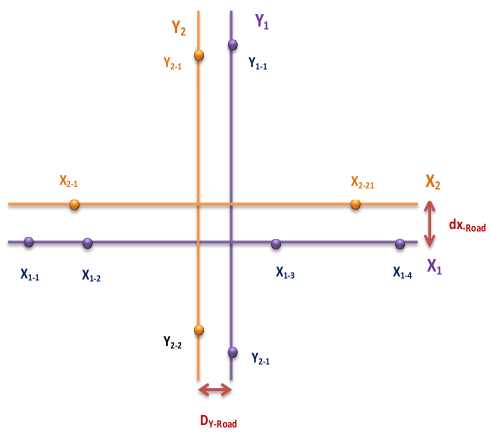
Regarding lanes modeling, there are two main approaches to model vehicles on multi-lane roads. The first approach, is the single lane abstraction model or simply the line abstraction model shown in Fig.4(a) in which all the traffic lanes are merged into a single lane with the aggregated traffic intensity (see Appendix.C in [28]). The second approach is to consider that the traffic is restricted into individual lanes separated by a fixed inter-lane distance, as illustrated in Fig.4(b). We will derive the outage probability for the two road scenario, then generalize the results for multiple lanes.

5.1 Two-lanes case scenario

We address the case where vehicles can drive in two opposite directions, on the horizontal roads and the vertical roads, and further on extend the analysis to Nblanes𝑁subscript𝑏𝑙𝑎𝑛𝑒𝑠Nb_{lanes} number of roads. We refer to the case when we have two roads in the horizontal, and two roads in the vertical as the two-way road case (two lanes on each road). In this case, the horizontal road on which vehicles drive from left to right (resp. right to left) is denoted X1subscript𝑋1X_{1} (resp. X2subscript𝑋2X_{2}). The same modification holds for the vertical road on which, vehicles drive from bottom up (resp. top down) is denoted Y1subscript𝑌1Y_{1} (resp. Y2subscript𝑌2Y_{2}). For α=2𝛼2\alpha=2, the expressions of the Laplace transform from the X1subscript𝑋1X_{1} road and the Y1subscript𝑌1Y_{1} road at the receiving node M𝑀M denoted respectively IX1M(s)subscriptsubscript𝐼subscriptsubscript𝑋1𝑀𝑠\mathcal{L}_{I_{{X_{1}}_{M}}}(s) and IY1M(s)subscriptsubscript𝐼subscriptsubscript𝑌1𝑀𝑠\mathcal{L}_{I_{{Y_{1}}_{M}}}(s), are given by (24) and (25). The expressions of the Laplace transform from the X2subscript𝑋2X_{2} road and from the Y2subscript𝑌2Y_{2} road at M𝑀M are given respectively by

IX2M(s)=exp(pλX2sπ(msin(θM)dYRoad)2+s),subscriptsubscript𝐼subscriptsubscript𝑋2𝑀𝑠psubscript𝜆subscript𝑋2𝑠𝜋superscript𝑚subscript𝜃𝑀subscript𝑑subscript𝑌𝑅𝑜𝑎𝑑2𝑠\mathcal{L}_{I_{{X_{2}}_{M}}}(s)=\exp\Bigg{(}-\emph{p}\lambda_{X_{2}}\dfrac{s\pi}{\sqrt{(m\sin(\theta_{M})-d_{Y_{Road}})^{2}+s}}\Bigg{)}, (24)

and

IY2M(s)=exp(pλY2sπ(mcos(θM)dXRoad)2+s),subscriptsubscript𝐼subscriptsubscript𝑌2𝑀𝑠psubscript𝜆subscript𝑌2𝑠𝜋superscript𝑚subscript𝜃𝑀subscript𝑑subscript𝑋𝑅𝑜𝑎𝑑2𝑠\mathcal{L}_{I_{{Y_{2}}_{M}}}(s)=\exp\Bigg{(}-\emph{p}\lambda_{Y_{2}}\dfrac{s\pi}{\sqrt{(m\cos(\theta_{M})-d_{X_{Road}})^{2}+s}}\Bigg{)}, (25)

where λX2subscript𝜆subscript𝑋2\lambda_{X_{2}} and λY2subscript𝜆subscript𝑌2\lambda_{Y_{2}} are the intensities of the interferer nodes on the X2subscript𝑋2X_{2} road and Y2subscript𝑌2Y_{2} road respectively, and dXRoadsubscript𝑑subscript𝑋𝑅𝑜𝑎𝑑d_{X_{Road}} and dYRoadsubscript𝑑subscript𝑌𝑅𝑜𝑎𝑑d_{Y_{Road}} are distance between X1subscript𝑋1X_{1} and X2subscript𝑋2X_{2}, and between Y1subscript𝑌1Y_{1} and Y2subscript𝑌2Y_{2} respectively.

proof: See B. \blacksquare

In the case when there are two roads on the vertical and two roads on the horizontal, the interference are generated from four roads, the outage probability of D1subscript𝐷1D_{1} and D2subscript𝐷2D_{2} become respectively

(O(1))=subscriptO1absent\displaystyle\mathbb{P}(\textit{O}_{(1)})=
1𝒥(D1)(2)(G1lSD1)𝒥(R)(2)(G1lSR)+𝒥(D1)(2)(G1lSD1)𝒥(R)(2)(G1lSR)1subscriptsuperscript𝒥2subscript𝐷1subscript𝐺1subscript𝑙𝑆subscript𝐷1subscriptsuperscript𝒥2𝑅subscript𝐺1subscript𝑙𝑆𝑅subscriptsuperscript𝒥2subscript𝐷1subscript𝐺1subscript𝑙𝑆subscript𝐷1subscriptsuperscript𝒥2𝑅subscript𝐺1subscript𝑙𝑆𝑅\displaystyle 1-\mathcal{J}^{(2)}_{(D_{1})}\big{(}\frac{G_{1}}{l_{SD_{1}}}\big{)}-\mathcal{J}^{(2)}_{(R)}\big{(}\frac{G_{1}}{l_{SR}}\big{)}+\mathcal{J}^{(2)}_{(D_{1})}\big{(}\frac{G_{1}}{l_{SD_{1}}}\big{)}\mathcal{J}^{(2)}_{(R)}\big{(}\frac{G_{1}}{l_{SR}}\big{)}
+𝒥(R)(2)(G1lSR)lRD1𝒥(R)(2)(G1lSR)𝒥(D1)(2)(G1lRD1)lSD1𝒥(R)(2)(G1lSR)𝒥(D1)(2)(G1lSD1)lRD1lSD1,subscriptsuperscript𝒥2𝑅subscript𝐺1subscript𝑙𝑆𝑅subscript𝑙𝑅subscript𝐷1subscriptsuperscript𝒥2𝑅subscript𝐺1subscript𝑙𝑆𝑅subscriptsuperscript𝒥2subscript𝐷1subscript𝐺1subscript𝑙𝑅subscript𝐷1subscript𝑙𝑆subscript𝐷1subscriptsuperscript𝒥2𝑅subscript𝐺1subscript𝑙𝑆𝑅subscriptsuperscript𝒥2subscript𝐷1subscript𝐺1subscript𝑙𝑆subscript𝐷1subscript𝑙𝑅subscript𝐷1subscript𝑙𝑆subscript𝐷1\displaystyle+\mathcal{J}^{(2)}_{(R)}\big{(}\frac{G_{1}}{l_{SR}}\big{)}-\frac{l_{RD_{1}}\mathcal{J}^{(2)}_{(R)}\big{(}\frac{G_{1}}{l_{SR}}\big{)}\mathcal{J}^{(2)}_{(D_{1})}\big{(}\frac{G_{1}}{l_{RD_{1}}}\big{)}-l_{SD_{1}}\mathcal{J}^{(2)}_{(R)}\big{(}\frac{G_{1}}{l_{SR}}\big{)}\mathcal{J}^{(2)}_{(D_{1})}\big{(}\frac{G_{1}}{l_{SD_{1}}}\big{)}}{l_{RD_{1}}-l_{SD_{1}}},

and

(O(2))=subscriptO2absent\displaystyle\mathbb{P}(\textit{O}_{(2)})=
1𝒥(D2)(2)(GmaxlSD2)𝒥(R)(2)(GmaxlSR)+𝒥(D2)(2)(GmaxlSD2)𝒥(R)(2)(GmaxlSR)1subscriptsuperscript𝒥2subscript𝐷2subscript𝐺maxsubscript𝑙𝑆subscript𝐷2subscriptsuperscript𝒥2𝑅subscript𝐺maxsubscript𝑙𝑆𝑅subscriptsuperscript𝒥2subscript𝐷2subscript𝐺maxsubscript𝑙𝑆subscript𝐷2subscriptsuperscript𝒥2𝑅subscript𝐺maxsubscript𝑙𝑆𝑅\displaystyle 1-\mathcal{J}^{(2)}_{(D_{2})}\big{(}\frac{G_{\mathrm{max}}}{l_{SD_{2}}}\big{)}-\mathcal{J}^{(2)}_{(R)}\big{(}\frac{G_{\mathrm{max}}}{l_{SR}}\big{)}+\mathcal{J}^{(2)}_{(D_{2})}\big{(}\frac{G_{\mathrm{max}}}{l_{SD_{2}}}\big{)}\mathcal{J}^{(2)}_{(R)}\big{(}\frac{G_{\mathrm{max}}}{l_{SR}}\big{)}
+𝒥(R)(2)(GmaxlSR)lRD2𝒥(R)(2)(GmaxlSR)𝒥(D2)(2)(GmaxlRD2)lSD2𝒥(R)(2)(GmaxlSR)𝒥(D2)(2)(GmaxlSD2)lRD2lSD2.subscriptsuperscript𝒥2𝑅subscript𝐺maxsubscript𝑙𝑆𝑅subscript𝑙𝑅subscript𝐷2subscriptsuperscript𝒥2𝑅subscript𝐺maxsubscript𝑙𝑆𝑅subscriptsuperscript𝒥2subscript𝐷2subscript𝐺maxsubscript𝑙𝑅subscript𝐷2subscript𝑙𝑆subscript𝐷2subscriptsuperscript𝒥2𝑅subscript𝐺maxsubscript𝑙𝑆𝑅subscriptsuperscript𝒥2subscript𝐷2subscript𝐺maxsubscript𝑙𝑆subscript𝐷2subscript𝑙𝑅subscript𝐷2subscript𝑙𝑆subscript𝐷2\displaystyle+\mathcal{J}^{(2)}_{(R)}\big{(}\frac{G_{\mathrm{max}}}{l_{SR}}\big{)}-\frac{l_{RD_{2}}\mathcal{J}^{(2)}_{(R)}\big{(}\frac{G_{\mathrm{max}}}{l_{SR}}\big{)}\mathcal{J}^{(2)}_{(D_{2})}\big{(}\frac{G_{\mathrm{max}}}{l_{RD_{2}}}\big{)}-l_{SD_{2}}\mathcal{J}^{(2)}_{(R)}\big{(}\frac{G_{\mathrm{max}}}{l_{SR}}\big{)}\mathcal{J}^{(2)}_{(D_{2})}\big{(}\frac{G_{\mathrm{max}}}{l_{SD_{2}}}\big{)}}{l_{RD_{2}}-l_{SD_{2}}}.

where the function is given by

𝒥(M)(2)(AB)=IXM(AB)IYM(AB)IX2M(AB)IY2M(AB)exp(σ2APB)2.\mathcal{J}^{(2)}_{(M)}\Big{(}\frac{A}{B}\Big{)}=\mathcal{L}_{I_{X_{M}}}\Big{(}\frac{A}{B}\Big{)}\mathcal{L}_{I_{Y_{M}}}\Big{(}\frac{A}{B}\Big{)}\mathcal{L}_{I_{{X_{2}}_{M}}}\Big{(}\frac{A}{B}\Big{)}\mathcal{L}_{I_{{Y_{2}}_{M}}}\Big{(}\frac{A}{B}\Big{)}\exp\Big{(}-\frac{\sigma^{2}A}{PB}\Big{)}^{2}.

5.2 Multi-lanes case scenario

To generalize the above expressions form Nblanes𝑁subscript𝑏𝑙𝑎𝑛𝑒𝑠Nb_{lanes} roads, we calculate the Laplace transform for the interference for ithXsuperscript𝑖𝑡𝑋i^{th}X road, and ithYsuperscript𝑖𝑡𝑌i^{th}Y road when α=2𝛼2\alpha=2 is respectively given by:

IXiM(s)=exp(pλXisπ(msin(θM)i=1Nblanes1(i1)dYRoad)2+s)subscriptsubscript𝐼subscriptsubscript𝑋𝑖𝑀𝑠psubscript𝜆subscript𝑋𝑖𝑠𝜋superscript𝑚subscript𝜃𝑀superscriptsubscript𝑖1𝑁subscript𝑏𝑙𝑎𝑛𝑒𝑠1𝑖1subscript𝑑subscript𝑌𝑅𝑜𝑎𝑑2𝑠\mathcal{L}_{I_{{X_{i}}_{M}}}(s)=\exp\Bigg{(}-\emph{p}\lambda_{X_{i}}\dfrac{s\pi}{\sqrt{(m\sin(\theta_{{M}})-\sum_{i=1}^{Nb_{lanes}-1}(i-1)d_{Y_{Road}})^{2}+s}}\Bigg{)} (26)
IYiM(s)=exp(pλYisπ(mcos(θM)i=1Nblanes1(i1)dXRoad)2+s)subscriptsubscript𝐼subscriptsubscript𝑌𝑖𝑀𝑠psubscript𝜆subscript𝑌𝑖𝑠𝜋superscript𝑚subscript𝜃𝑀superscriptsubscript𝑖1𝑁subscript𝑏𝑙𝑎𝑛𝑒𝑠1𝑖1subscript𝑑subscript𝑋𝑅𝑜𝑎𝑑2𝑠\mathcal{L}_{I_{{Y_{i}}_{M}}}(s)=\exp\Bigg{(}-\emph{p}\lambda_{Y_{i}}\dfrac{s\pi}{\sqrt{(m\cos(\theta_{{M}})-\sum_{i=1}^{Nb_{lanes}-1}(i-1)d_{X_{Road}})^{2}+s}}\Bigg{)} (27)

where λXisubscript𝜆subscript𝑋𝑖\lambda_{X_{i}} and λYisubscript𝜆subscript𝑌𝑖\lambda_{Y_{i}} are the intensities of the interferer nodes on the Xisubscript𝑋𝑖X_{i} road and Yisubscript𝑌𝑖Y_{i} road respectively. Hence the outage probability of D1subscript𝐷1D_{1} and D2subscript𝐷2D_{2} are respectively given by

(O(1))=subscriptO1absent\displaystyle\mathbb{P}(\textit{O}_{(1)})=
1𝒥(D1)(Nblanes)(G1lSD1)𝒥(R)(Nblanes)(G1lSR)+𝒥(D1)(Nblanes)(G1lSD1)𝒥(R)(Nblanes)(G1lSR)1subscriptsuperscript𝒥𝑁subscript𝑏𝑙𝑎𝑛𝑒𝑠subscript𝐷1subscript𝐺1subscript𝑙𝑆subscript𝐷1subscriptsuperscript𝒥𝑁subscript𝑏𝑙𝑎𝑛𝑒𝑠𝑅subscript𝐺1subscript𝑙𝑆𝑅subscriptsuperscript𝒥𝑁subscript𝑏𝑙𝑎𝑛𝑒𝑠subscript𝐷1subscript𝐺1subscript𝑙𝑆subscript𝐷1subscriptsuperscript𝒥𝑁subscript𝑏𝑙𝑎𝑛𝑒𝑠𝑅subscript𝐺1subscript𝑙𝑆𝑅\displaystyle 1-\mathcal{J}^{(Nb_{lanes})}_{(D_{1})}\big{(}\frac{G_{1}}{l_{SD_{1}}}\big{)}-\mathcal{J}^{(Nb_{lanes})}_{(R)}\big{(}\frac{G_{1}}{l_{SR}}\big{)}+\mathcal{J}^{(Nb_{lanes})}_{(D_{1})}\big{(}\frac{G_{1}}{l_{SD_{1}}}\big{)}\mathcal{J}^{(Nb_{lanes})}_{(R)}\big{(}\frac{G_{1}}{l_{SR}}\big{)}
+𝒥(R)(Nblanes)(G1lSR)subscriptsuperscript𝒥𝑁subscript𝑏𝑙𝑎𝑛𝑒𝑠𝑅subscript𝐺1subscript𝑙𝑆𝑅\displaystyle+\mathcal{J}^{(Nb_{lanes})}_{(R)}\big{(}\frac{G_{1}}{l_{SR}}\big{)}
lRD1𝒥(R)(Nblanes)(G1lSR)𝒥(D1)(Nblanes)(G1lRD1)lSD1𝒥(R)(Nblanes)(G1lSR)𝒥(D1)(Nblanes)(G1lSD1)lRD1lSD1,subscript𝑙𝑅subscript𝐷1subscriptsuperscript𝒥𝑁subscript𝑏𝑙𝑎𝑛𝑒𝑠𝑅subscript𝐺1subscript𝑙𝑆𝑅subscriptsuperscript𝒥𝑁subscript𝑏𝑙𝑎𝑛𝑒𝑠subscript𝐷1subscript𝐺1subscript𝑙𝑅subscript𝐷1subscript𝑙𝑆subscript𝐷1subscriptsuperscript𝒥𝑁subscript𝑏𝑙𝑎𝑛𝑒𝑠𝑅subscript𝐺1subscript𝑙𝑆𝑅subscriptsuperscript𝒥𝑁subscript𝑏𝑙𝑎𝑛𝑒𝑠subscript𝐷1subscript𝐺1subscript𝑙𝑆subscript𝐷1subscript𝑙𝑅subscript𝐷1subscript𝑙𝑆subscript𝐷1\displaystyle-\frac{l_{RD_{1}}\mathcal{J}^{(Nb_{lanes})}_{(R)}\big{(}\frac{G_{1}}{l_{SR}}\big{)}\mathcal{J}^{(Nb_{lanes})}_{(D_{1})}\big{(}\frac{G_{1}}{l_{RD_{1}}}\big{)}-l_{SD_{1}}\mathcal{J}^{(Nb_{lanes})}_{(R)}\big{(}\frac{G_{1}}{l_{SR}}\big{)}\mathcal{J}^{(Nb_{lanes})}_{(D_{1})}\big{(}\frac{G_{1}}{l_{SD_{1}}}\big{)}}{l_{RD_{1}}-l_{SD_{1}}}, (28)

and

(O(2))=subscriptO2absent\displaystyle\mathbb{P}(\textit{O}_{(2)})=
1𝒥(D2)(Nblanes)(GmaxlSD2)𝒥(R)(Nblanes)(GmaxlSR)+𝒥(D2)(Nblanes)(GmaxlSD2)𝒥(R)(Nblanes)(GmaxlSR)1subscriptsuperscript𝒥𝑁subscript𝑏𝑙𝑎𝑛𝑒𝑠subscript𝐷2subscript𝐺maxsubscript𝑙𝑆subscript𝐷2subscriptsuperscript𝒥𝑁subscript𝑏𝑙𝑎𝑛𝑒𝑠𝑅subscript𝐺maxsubscript𝑙𝑆𝑅subscriptsuperscript𝒥𝑁subscript𝑏𝑙𝑎𝑛𝑒𝑠subscript𝐷2subscript𝐺maxsubscript𝑙𝑆subscript𝐷2subscriptsuperscript𝒥𝑁subscript𝑏𝑙𝑎𝑛𝑒𝑠𝑅subscript𝐺maxsubscript𝑙𝑆𝑅\displaystyle 1-\mathcal{J}^{(Nb_{lanes})}_{(D_{2})}\big{(}\frac{G_{\mathrm{max}}}{l_{SD_{2}}}\big{)}-\mathcal{J}^{(Nb_{lanes})}_{(R)}\big{(}\frac{G_{\mathrm{max}}}{l_{SR}}\big{)}+\mathcal{J}^{(Nb_{lanes})}_{(D_{2})}\big{(}\frac{G_{\mathrm{max}}}{l_{SD_{2}}}\big{)}\mathcal{J}^{(Nb_{lanes})}_{(R)}\big{(}\frac{G_{\mathrm{max}}}{l_{SR}}\big{)}
+𝒥(R)(Nblanes)(GmaxlSR)subscriptsuperscript𝒥𝑁subscript𝑏𝑙𝑎𝑛𝑒𝑠𝑅subscript𝐺maxsubscript𝑙𝑆𝑅\displaystyle+\mathcal{J}^{(Nb_{lanes})}_{(R)}\big{(}\frac{G_{\mathrm{max}}}{l_{SR}}\big{)}
lRD2𝒥(R)(Nblanes)(GmaxlSR)𝒥(D2)(Nblanes)(GmaxlRD2)lSD2𝒥(R)(Nblanes)(GmaxlSR)𝒥(D2)(Nblanes)(GmaxlSD2)lRD2lSD2.subscript𝑙𝑅subscript𝐷2subscriptsuperscript𝒥𝑁subscript𝑏𝑙𝑎𝑛𝑒𝑠𝑅subscript𝐺maxsubscript𝑙𝑆𝑅subscriptsuperscript𝒥𝑁subscript𝑏𝑙𝑎𝑛𝑒𝑠subscript𝐷2subscript𝐺maxsubscript𝑙𝑅subscript𝐷2subscript𝑙𝑆subscript𝐷2subscriptsuperscript𝒥𝑁subscript𝑏𝑙𝑎𝑛𝑒𝑠𝑅subscript𝐺maxsubscript𝑙𝑆𝑅subscriptsuperscript𝒥𝑁subscript𝑏𝑙𝑎𝑛𝑒𝑠subscript𝐷2subscript𝐺maxsubscript𝑙𝑆subscript𝐷2subscript𝑙𝑅subscript𝐷2subscript𝑙𝑆subscript𝐷2\displaystyle-\frac{l_{RD_{2}}\mathcal{J}^{(Nb_{lanes})}_{(R)}\big{(}\frac{G_{\mathrm{max}}}{l_{SR}}\big{)}\mathcal{J}^{(Nb_{lanes})}_{(D_{2})}\big{(}\frac{G_{\mathrm{max}}}{l_{RD_{2}}}\big{)}-l_{SD_{2}}\mathcal{J}^{(Nb_{lanes})}_{(R)}\big{(}\frac{G_{\mathrm{max}}}{l_{SR}}\big{)}\mathcal{J}^{(Nb_{lanes})}_{(D_{2})}\big{(}\frac{G_{\mathrm{max}}}{l_{SD_{2}}}\big{)}}{l_{RD_{2}}-l_{SD_{2}}}. (29)

where

𝒥(M)(Nblanes)(AB)=exp(σ2APB)Nblanes×i=1NblanesIXiM(AB)IYiM(AB).\mathcal{J}^{(Nb_{lanes})}_{(M)}\Big{(}\frac{A}{B}\Big{)}=\exp\Big{(}-\frac{\sigma^{2}A}{PB}\Big{)}^{Nb_{lanes}}\times\prod_{i=1}^{{Nb_{lanes}}}\mathcal{L}_{I_{{X_{i}}_{M}}}\Big{(}\frac{A}{B}\Big{)}\mathcal{L}_{I_{{Y_{i}}_{M}}}\Big{(}\frac{A}{B}\Big{)}. (30)
Refer to caption
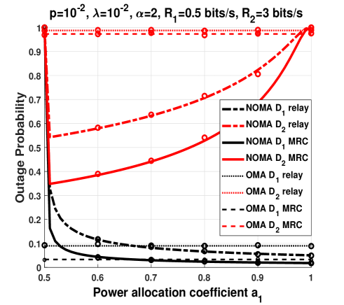
Figure 5: Outage probability as a function of a1subscript𝑎1a_{1} considering NOMA and OMA.

6 Simulations and Discussions

In this section, we evaluate the performance of MRC with NOMA at road intersections. Monte-Carlo simulation are carried out by generating samples (which correspond to the interfering vehicles) according to a PPP, and we average over 50,0005000050,000 iterations of Rayleigh fading channel coefficients. The Monte-Carlo simulations match the theoretical analysis, which confirm the accuracy of our results. Unless stated otherwise, β=0𝛽0\beta=0, S=[100,0]𝑆1000S=[100,0], R=[50,0]𝑅500R=[50,0], D1=[0,0]subscript𝐷100D_{1}=[0,0] and D2=[0,10]subscript𝐷2010D_{2}=[0,-10]. We set, without loss of generality, λX=λY=λsubscript𝜆𝑋subscript𝜆𝑌𝜆\lambda_{X}=\lambda_{Y}=\lambda.

Refer to caption
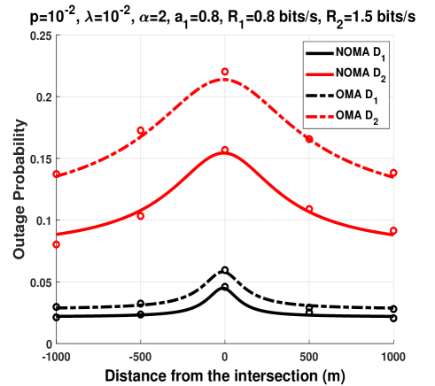
Figure 6: Outage probability as a function of the distance from the intersection considering NOMA and OMA.

Fig.5 compares the outage probability as a function of a1subscript𝑎1a_{1}, considering a NOMA relay transmission [41], NOMA MRC transmission (the proposed method), OMA relay transmission, and OMA MRC transmission [35]. The figure shows that implementing MRC with NOMA offers a significant improvement on the performance compared to the relay transmission. This improvement is event greater for D2subscript𝐷2D_{2}. To quantify this improvement, we notice that, MRC with NOMA offers decrease of the outage probability of 34%percent3434\% compared to the relay transmission with NOMA. Whereas the improvement of MRC with OMA is 2%percent22\% compared to the relay transmission with OMA. We can also notice that there is an improvement of 60%percent6060\% in terms of outage probability when using MRC with NOMA compared to MRC with OMA.

Fig.6 depicts the outage probability as a function of the distance between the nodes and the intersection. We can see, from Fig.6, that the outage probability has a peak at the intersection. This can be explained by the fact that the interfering vehicles from both X𝑋X and Y𝑌Y road contribute to the aggregate interference. Whereas only one road contribute to the aggregate interference when the nodes are far from the intersection. We also see that implementing MRC with NOMA offers a better performance than MRC with OMA for D1subscript𝐷1D_{1} and D2subscript𝐷2D_{2}.

Refer to caption
Figure 7: Outage probability as a function of λ𝜆\lambda considering NOMA and OMA.

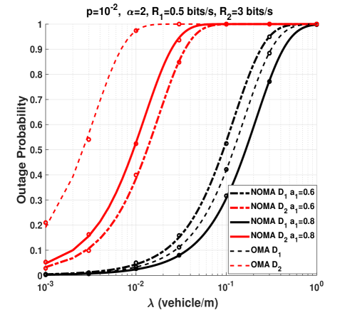
Fig.7 plots the outage probability as a function of the vehicles density λ𝜆\lambda. We notice that as the intensity of the interfering vehicles increases, the outage probability increases. The reason is that as the number of vehicles increases, the aggregate of interference increases at the receiver node, which decreases the SIR and increases the outage probability. Note that the value of a1subscript𝑎1a_{1} has to be chosen carefully, since when a1=0.6subscript𝑎10.6a_{1}=0.6, MRC with NOMA offers a better performance than MRC with OMA for D1subscript𝐷1D_{1} and D2subscript𝐷2D_{2}. which is not the case when a1=0.8subscript𝑎10.8a_{1}=0.8

Refer to caption
Figure 8: Outage probability as a function of λ𝜆\lambda considering NOMA using different transmission schemes.

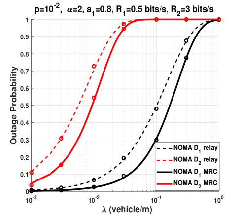
Fig.8 shows the outage probability as a function of λ𝜆\lambda considering NOMA using different transmission schemes. We can clearly see that the MRC using NOMA outperforms the classical relay transmission using NOMA. This holds true for both D1subscript𝐷1D_{1} and D2subscript𝐷2D_{2}. This result is intuitive since in the relay transmission using NOMA, D1subscript𝐷1D_{1} and D2subscript𝐷2D_{2} decode the message transmitted by the relay. However, in the MRC transmission scheme using NOMA, D1subscript𝐷1D_{1} and D2subscript𝐷2D_{2} combine the signal from the source, and from the relay, which increases the power at the D1subscript𝐷1D_{1} and D2subscript𝐷2D_{2}, and consequently increases the SINR.
Refer to caption
(a)
Refer to caption
(b)
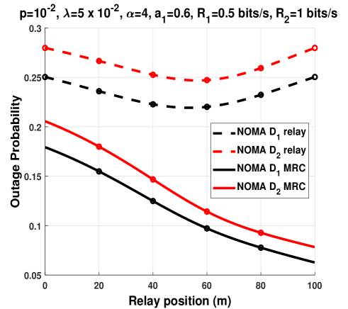
Figure 9: Outage probability as a function of the relay position. (a) α=2𝛼2\alpha=2. (a) α=4𝛼4\alpha=4.

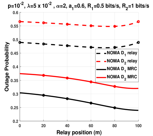
Fig.9 depicts the outage probability as a function of the relay position, using a relay transmission and MRC transmission considering NOMA. We set, without loss of generality, SD1=SD2=100norm𝑆subscript𝐷1norm𝑆subscript𝐷2100\|S-D_{1}\|=\|S-D_{2}\|=100m.

We can notice from Fig.9(a) that when α=2𝛼2\alpha=2, the optimal position for the relay using a relay transmission is near the destinations, D1subscript𝐷1D_{1} and D2subscript𝐷2D_{2}, whereas for MRC, the optimal relay position is when the relay is close to the destination nodes.

When α=4𝛼4\alpha=4, we can see, from Fig.9(b), that the best position for the relay is at mid-distance between S𝑆S and the destination nodes when using the relay transmission. But, when using MRC, the best relay position is when the relay is near the destination nodes. This is because, when the relay is near the destination, the channel coefficients between and S𝑆S and the destination, and between R𝑅R and the destination are decorrelated, which increases the diversity gain.
Refer to caption
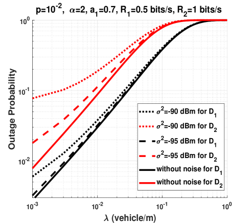
Figure 10: Outage probability as a function of λ𝜆\lambda for several noise power values.

We can see form the Fig.10 that the noise power greatly impact the performance only for low values of λ𝜆\lambda. However, as the value of λ𝜆\lambda increases, the performance when considering noise power and without noise power tends the same values. This because for high value of λ𝜆\lambda, the power of noise become negligible compared to the power of interference.

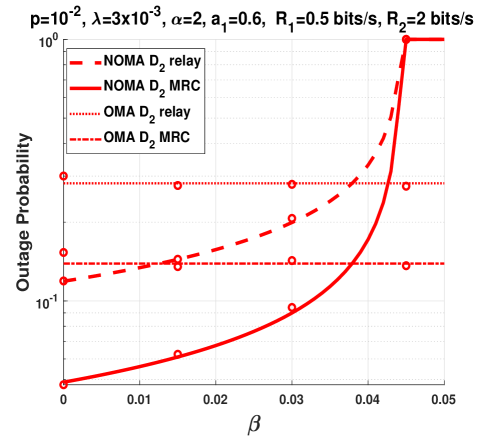
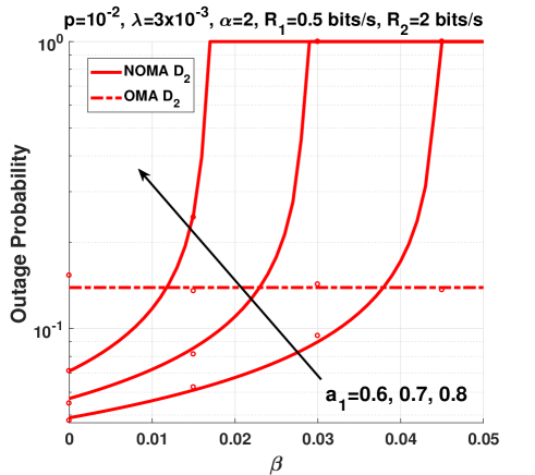
Fig.11 shows the impact of β𝛽\beta on the performance in terms of outage probability. We can see from Fig.11(a) that for low values of β𝛽\beta the outage probability considering NOMA is lower than OMA when using MRC transmission. However, as the value of β𝛽\beta increases, the outage probability of NOMA increases. We can also see that as a1subscript𝑎1a_{1} decreases, the values of the effect of β𝛽\beta becomes less dominant. This because as we allocate more power to D2subscript𝐷2D_{2}, it increases the SINR at D2subscript𝐷2D_{2} hence decreasing the outage probability. We can also see from Fig.11(b) that the MRC outperforms the relay transmission for both NOMA and OMA. However, we can see that the value of β𝛽\beta when OMA outperforms NOMA is the same for MRC and the relay transmission.
Refer to caption
(a)
Refer to caption
(b)
Figure 11: Outage probability of D2subscript𝐷2D_{2} as a function of β𝛽\beta considering NOMA and OMA. (a) NOMA and OMA considering MRC transmission. (b) NOMA and OMA considering MRC transmission and relay transmission.
Refer to caption
(a)
Refer to caption
(b)
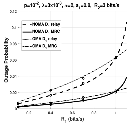
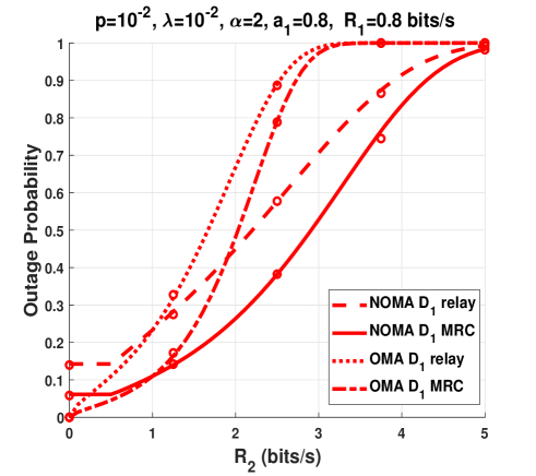
Figure 12: Outage probability as a function of data rate considering NOMA and OMA. (a) Outage probability as a function of 1subscript1\mathcal{R}_{1}. (b) Outage probability as a function of 2subscript2\mathcal{R}_{2}.
Refer to caption
(a)
Refer to caption
(b)
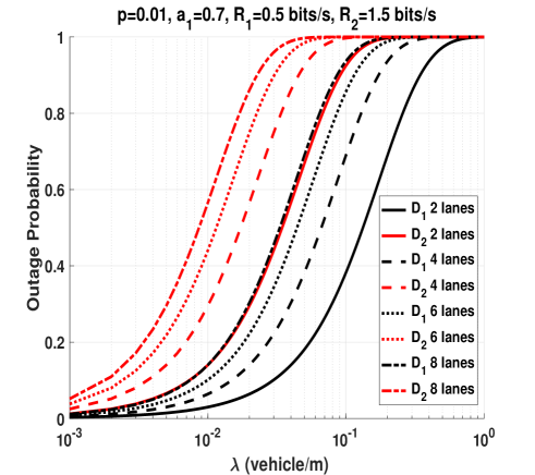
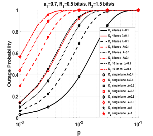
Figure 13: Multiple lanes modeling considering MRC NOMA. (a) outage probability as a function of λ𝜆\lambda for Nblane={2,4,6,8}𝑁subscript𝑏𝑙𝑎𝑛𝑒2468Nb_{lane}=\{2,4,6,8\}. (b) outage probability as a function of p𝑝p for the single lane model and the multiple lane model for several values of Nblane𝑁subscript𝑏𝑙𝑎𝑛𝑒Nb_{lane}.

Finally, we investigate the impact of the data rates 1subscript1\mathcal{R}_{1} and 2subscript2\mathcal{R}_{2} on the performance considering NOMA and OMA using MRC and the relay transmission. We can see from Fig.12(a) that as 1subscript1\mathcal{R}_{1} increases, the outage probability of D1subscript𝐷1D_{1} increases. This is intuitive since increasing the data rate increases the decoding threshold which increases the outage probability. We can also see that NOMA offers better performance than OMA. However, as 1subscript1\mathcal{R}_{1} increases, OMA outperforms NOMA for both MRC transmission and relay transmission.

Also, we can see from Fig.12(b) that from small values of 2subscript2\mathcal{R}_{2}, that is, 2<0.5subscript20.5\mathcal{R}_{2}<0.5 bit/s, OMA offers better performance than NOMA in terms of outage probability. This is because, unlike the vehicle D1subscript𝐷1D_{1}, the vehicle D2subscript𝐷2D_{2} has to decode D1subscript𝐷1D_{1} message first, and then decode its own message. Hence, (D2)subscript𝐷2\mathbb{P}(D_{2}) depends solely on 1subscript1\mathcal{R}_{1} for small values of 2subscript2\mathcal{R}_{2}. We also notice that, for large values of 2subscript2\mathcal{R}_{2} (2>2bit/s)subscript22bit/s(\mathcal{R}_{2}>2\textrm{bit/s}), NOMA has better performance in terms of outage probability than OMA. This because for large values of 2subscript2\mathcal{R}_{2}, the decoding threshold of OMA increases linearly since it is multiplied by a factor of 4. This proves that cooperative NOMA has a better outage performance for high data rates. Finally, we can see that MRC transmission outperforms cooperative transmission for both NOMA and OMA.

Fig.13(a) plots NOMA outage probability as a function of λ𝜆\lambda for considering MRC for several values of Nblane𝑁subscript𝑏𝑙𝑎𝑛𝑒Nb_{lane}. We can see an increases in the outage probability as the number of lanes increases. This results is intuitive because when the number of lanes increases the interfering vehicles density increases as well, hence increasing the outage probability. Fig.13(b) shows NOMA outage probability as a function of p𝑝p using NOMA and considering the 1D-HPPP with a single lanes model, and the 1D-HPPP with multiple lanes. We can see from the Fig.13(b) that the single lane model matches perfectly the multiple lanes model.

7 Conclusion

In this paper, we implemented MRC using NOMA in VCs at road intersections. We derived closed form expressions of the outage probability for a setup involving two destinations. Then we extended the analysis for a scenario involving K𝐾K destinations. We also analyzed the performance for several road lanes. We noticed that implementing MRC using NOMA in vehicles improvements significantly the performance. compared to the standard cooperative transmission using NOMA. We also noticed that MRC using NOMA significantly outperforms MRC using OMA. From our results we concluded that it is always beneficial to use MRC and NOMA even at the cost of implementation complexity. Finally, we demonstrated that the outage probability has a peak when the vehicles are at the intersection, and that using MRC considering NOMA offers a great improvement in this context.

Appendix A

The outage probability related to D1subscript𝐷1D_{1}, denoted (O(1))subscriptO1\mathbb{P}(\textit{O}_{(1)}), is expressed as

(O(1))=(D1𝒜D1)+(𝒜D1C𝒞D1).subscriptO1subscriptsubscript𝐷1subscript𝒜subscript𝐷1superscriptsubscript𝒜subscript𝐷1𝐶subscript𝒞subscript𝐷1\mathbb{P}(\textit{O}_{(1)})=\mathbb{P}\Big{(}\mathcal{B}_{D_{1}}\cap\mathcal{A}_{D_{1}}\Big{)}+\mathbb{P}\Big{(}\mathcal{A}_{D_{1}}^{C}\cap\mathcal{C}_{D_{1}}\Big{)}. (31)

First, we calculate the probability (𝒜R1C𝒞D1)superscriptsubscript𝒜subscript𝑅1𝐶subscript𝒞subscript𝐷1\mathbb{P}\Big{(}\mathcal{A}_{R_{1}}^{C}\cap\mathcal{C}_{D_{1}}\Big{)} as follows

(𝒜R1C𝒞D1)superscriptsubscript𝒜subscript𝑅1𝐶subscript𝒞subscript𝐷1\displaystyle\mathbb{P}\Big{(}\mathcal{A}_{R_{1}}^{C}\cap\mathcal{C}_{D_{1}}\Big{)}
=𝔼IX,IY[{P|hSR|2lSRa1P|hSR|2lSRa2+IXR+IYR+σ2Θ1\displaystyle=\mathbb{E}_{I_{X},I_{Y}}\Bigg{[}\mathbb{P}\Bigg{\{}\ \frac{P|h_{SR}|^{2}l_{SR}a_{1}}{P|h_{SR}|^{2}l_{SR}a_{2}+I_{X_{R}}+I_{Y_{R}}+\sigma^{2}}\geq\Theta_{1}
P(|hSD1|2lSD1+|hRD1|2lRD1)a1P(|hSD1|2lSD1+|hRD1|2lRD1)a2+IXD1+IYD1+σ2<Θ1}]\displaystyle\quad\quad\quad\bigcap\frac{P\left(|h_{SD_{1}}|^{2}l_{SD_{1}}+|h_{RD_{1}}|^{2}l_{RD_{1}}\right)\,a_{1}}{P\left(|h_{SD_{1}}|^{2}l_{SD_{1}}+|h_{RD_{1}}|^{2}l_{RD_{1}}\right)\,a_{2}+I_{X_{D_{1}}}+I_{Y_{D_{1}}}+\sigma^{2}}<\Theta_{1}\Bigg{\}}\Bigg{]}
=\displaystyle= 𝔼IX,IY[{P|hSR|2lSR(a1Θ1a2)Θ1[IXR+IYR+σ2]\displaystyle\mathbb{E}_{I_{X},I_{Y}}\Bigg{[}\mathbb{P}\Bigg{\{}\ P|h_{SR}|^{2}l_{SR}(a_{1}-\Theta_{1}a_{2})\geq\Theta_{1}\big{[}I_{X_{R}}+I_{Y_{R}}+\sigma^{2}\big{]}
P(|hSD1|2lSD1+|hRD1|2lRD1)(a1Θ1a2)<Θ1[IXD1+IYD1+σ2]}].\displaystyle\quad\bigcap P\left(|h_{SD_{1}}|^{2}l_{SD_{1}}+|h_{RD_{1}}|^{2}l_{RD_{1}}\right)\,(a_{1}-\Theta_{1}a_{2})<\Theta_{1}\big{[}I_{X_{D_{1}}}+I_{Y_{D_{1}}}+\sigma^{2}\big{]}\Bigg{\}}\Bigg{]}.

When Θ1<a1/a2subscriptΘ1subscript𝑎1subscript𝑎2\Theta_{1}<a_{1}/a_{2}, and after setting G1=Θ1/(a1Θ1a2)subscript𝐺1subscriptΘ1subscript𝑎1subscriptΘ1subscript𝑎2G_{1}=\Theta_{1}/(a_{1}-\Theta_{1}a_{2}), then

(𝒜R1C𝒞D1)superscriptsubscript𝒜subscript𝑅1𝐶subscript𝒞subscript𝐷1\displaystyle\mathbb{P}\Big{(}\mathcal{A}_{R_{1}}^{C}\cap\mathcal{C}_{D_{1}}\Big{)}
=𝔼IX,IY[{|hSR|2G1lSR[IXR+IYR+σ2/P]\displaystyle=\mathbb{E}_{I_{X},I_{Y}}\Bigg{[}\mathbb{P}\Bigg{\{}\ |h_{SR}|^{2}\geq\frac{G_{1}}{l_{SR}}\big{[}I_{X_{R}}+I_{Y_{R}}+\sigma^{2}/P\big{]}
(|hSD1|2lSD1+|hRD1|2lRD1)<G1[IXD1+IYD1+σ2/P]}].\displaystyle\qquad\qquad\bigcap\left(|h_{SD_{1}}|^{2}l_{SD_{1}}+|h_{RD_{1}}|^{2}l_{RD_{1}}\right)<G_{1}\big{[}I_{X_{D_{1}}}+I_{Y_{D_{1}}}+\sigma^{2}/P\big{]}\Bigg{\}}\Bigg{]}. (33)

Since |hSR|2superscriptsubscript𝑆𝑅2|h_{SR}|^{2} follows an exponential distribution with unit mean, we get

(𝒜R1C𝒞D1)=𝔼IX,IY[{exp(G1lSR[IXR+IYR+σ2/P])}×1{(|hSD1|2lSD1+|hRD1|2lRD1)G1[IXD1+IYD1+σ2/P]}].superscriptsubscript𝒜subscript𝑅1𝐶subscript𝒞subscript𝐷1subscript𝔼subscript𝐼𝑋subscript𝐼𝑌delimited-[]subscript𝐺1subscript𝑙𝑆𝑅delimited-[]subscript𝐼subscript𝑋𝑅subscript𝐼subscript𝑌𝑅superscript𝜎2𝑃1superscriptsubscript𝑆subscript𝐷12subscript𝑙𝑆subscript𝐷1superscriptsubscript𝑅subscript𝐷12subscript𝑙𝑅subscript𝐷1subscript𝐺1delimited-[]subscript𝐼subscript𝑋subscript𝐷1subscript𝐼subscript𝑌subscript𝐷1superscript𝜎2𝑃\mathbb{P}\Big{(}\mathcal{A}_{R_{1}}^{C}\cap\mathcal{C}_{D_{1}}\Big{)}=\mathbb{E}_{I_{X},I_{Y}}\Bigg{[}\mathbb{P}\Bigg{\{}\ \exp\left(\frac{G_{1}}{l_{SR}}\big{[}I_{X_{R}}+I_{Y_{R}}+\sigma^{2}/P\big{]}\right)\Bigg{\}}\\ \times 1-\Bigg{\{}\mathbb{P}\left(|h_{SD_{1}}|^{2}l_{SD_{1}}+|h_{RD_{1}}|^{2}l_{RD_{1}}\right)\geq G_{1}\big{[}I_{X_{D_{1}}}+I_{Y_{D_{1}}}+\sigma^{2}/P\big{]}\Bigg{\}}\Bigg{]}. (34)

We write the second probability in (34) as

(δG1[IXD1+IYD1+σ2/P]),𝛿subscript𝐺1delimited-[]subscript𝐼subscript𝑋subscript𝐷1subscript𝐼subscript𝑌subscript𝐷1superscript𝜎2𝑃\mathbb{P}(\delta\geq G_{1}[I_{X_{D_{1}}}+I_{Y_{D_{1}}}+\sigma^{2}/P]),

where δ=|hRD1|2lRD1+|hSD1|2lSD1𝛿superscriptsubscript𝑅subscript𝐷12subscript𝑙𝑅subscript𝐷1superscriptsubscript𝑆subscript𝐷12subscript𝑙𝑆subscript𝐷1\delta=|h_{RD_{1}}|^{2}l_{RD_{1}}+|h_{SD_{1}}|^{2}l_{SD_{1}}.
The complementary cumulative distribution function of the random variable δ𝛿\delta, denoted F¯δ(.)\bar{F}_{\delta}(.), is given by

F¯δ(u)=lRD1eu/lRD1lSD1eu/lSD1lRD1lSD1subscript¯𝐹𝛿𝑢subscript𝑙𝑅subscript𝐷1superscript𝑒𝑢subscript𝑙𝑅subscript𝐷1subscript𝑙𝑆subscript𝐷1superscript𝑒𝑢subscript𝑙𝑆subscript𝐷1subscript𝑙𝑅subscript𝐷1subscript𝑙𝑆subscript𝐷1\bar{F}_{\delta}(u)=\dfrac{l_{RD_{1}}e^{-u/l_{RD_{1}}}-l_{SD_{1}}e^{-u/l_{SD_{1}}}}{l_{RD_{1}}-l_{SD_{1}}}.

Then, we have

[|hSD1|2lSD1+|hRD1|2lRD1G1(IXD1+IYD1+σ2/P)]=lRD1exp[G1lRD1(IXD1+IYD1+σ2/P)]lSD1exp(G1lSD1[IXD1+IYD1+σ2/P)]lRD1lSD1,\mathbb{P}\big{[}|h_{SD_{1}}|^{2}l_{SD_{1}}+|h_{RD_{1}}|^{2}l_{RD_{1}}\geq G_{1}(I_{X_{D_{1}}}+I_{Y_{D_{1}}}+\sigma^{2}/P)\big{]}=\\ \dfrac{l_{RD_{1}}\exp\Big{[}-\dfrac{G_{1}}{l_{RD_{1}}}(I_{X_{D_{1}}}+I_{Y_{D_{1}}}+\sigma^{2}/P)\Big{]}-l_{SD_{1}}\exp\Big{(}-\dfrac{G_{1}}{l_{SD_{1}}}[I_{X_{D_{1}}}+I_{Y_{D_{1}}}+\sigma^{2}/P)\Big{]}}{l_{RD_{1}}-l_{SD_{1}}}, (35)

Plugging (35) into (34) yields

(𝒜R1C𝒞D1)=superscriptsubscript𝒜subscript𝑅1𝐶subscript𝒞subscript𝐷1absent\displaystyle\mathbb{P}\Big{(}\mathcal{A}_{R_{1}}^{C}\cap\mathcal{C}_{D_{1}}\Big{)}=
𝔼IX,IY[exp(G1lSR[IXR+IYR+σ2/P])\displaystyle\mathbb{E}_{I_{X},I_{Y}}\Bigg{[}\exp\left(\frac{G_{1}}{l_{SR}}\big{[}I_{X_{R}}+I_{Y_{R}}+\sigma^{2}/P\big{]}\right)
×{1lRD1exp(G1lRD1(IXD1+IYD1+σ2/P))lRD1lSD1\displaystyle\qquad\times\Bigg{\{}1-\dfrac{l_{RD_{1}}\exp\Big{(}-\dfrac{G_{1}}{l_{RD_{1}}}(I_{X_{D_{1}}}+I_{Y_{D_{1}}}+\sigma^{2}/P)\Big{)}}{l_{RD_{1}}-l_{SD_{1}}}
lSD1exp(G1lSD1[IXD1+IYD1+σ2/P])lRD1lSD1}]\displaystyle\qquad-\dfrac{l_{SD_{1}}\exp\Big{(}-\dfrac{G_{1}}{l_{SD_{1}}}[I_{X_{D_{1}}}+I_{Y_{D_{1}}}+\sigma^{2}/P]\Big{)}}{l_{RD_{1}}-l_{SD_{1}}}\Bigg{\}}\Bigg{]}
=\displaystyle= 𝔼IX,IY[exp(G1lSR[IXR+IYR+σ2/P])exp(G1lSR[IXR+IYR+σ2/P])\displaystyle\mathbb{E}_{I_{X},I_{Y}}\Bigg{[}\exp\left(\frac{G_{1}}{l_{SR}}\big{[}I_{X_{R}}+I_{Y_{R}}+\sigma^{2}/P\big{]}\right)-\exp\left(\frac{G_{1}}{l_{SR}}\big{[}I_{X_{R}}+I_{Y_{R}}+\sigma^{2}/P\big{]}\right)
×lRD1exp(G1lRD1[IXD1+IYD1+σ2/P])lRD1lSD1absentsubscript𝑙𝑅subscript𝐷1subscript𝐺1subscript𝑙𝑅subscript𝐷1delimited-[]subscript𝐼subscript𝑋subscript𝐷1subscript𝐼subscript𝑌subscript𝐷1superscript𝜎2𝑃subscript𝑙𝑅subscript𝐷1subscript𝑙𝑆subscript𝐷1\displaystyle\qquad\times\dfrac{l_{RD_{1}}\exp\Big{(}-\dfrac{G_{1}}{l_{RD_{1}}}[I_{X_{D_{1}}}+I_{Y_{D_{1}}}+\sigma^{2}/P]\Big{)}}{l_{RD_{1}}-l_{SD_{1}}}
lSD1exp(G1lSD1[IXD1+IYD1+σ2/P])lRD1lSD1)].\displaystyle\qquad-\dfrac{l_{SD_{1}}\exp\Big{(}-\dfrac{G_{1}}{l_{SD_{1}}}[I_{X_{D_{1}}}+I_{Y_{D_{1}}}+\sigma^{2}/P]\Big{)}}{l_{RD_{1}}-l_{SD_{1}}}\big{)}\Bigg{]}.

Given that 𝔼[esI]=I(s)𝔼delimited-[]superscript𝑒𝑠𝐼subscript𝐼𝑠\mathbb{E}[e^{sI}]=\mathcal{L}_{I}(s), we finally get

(𝒜R1C𝒞D1)=superscriptsubscript𝒜subscript𝑅1𝐶subscript𝒞subscript𝐷1absent\displaystyle\mathbb{P}\Big{(}\mathcal{A}_{R_{1}}^{C}\cap\mathcal{C}_{D_{1}}\Big{)}= IXR(G1lSR)IYR(G1lSR)exp(σ2G1PlSR)subscriptsubscript𝐼subscript𝑋𝑅subscript𝐺1subscript𝑙𝑆𝑅subscriptsubscript𝐼subscript𝑌𝑅subscript𝐺1subscript𝑙𝑆𝑅superscript𝜎2subscript𝐺1𝑃subscript𝑙𝑆𝑅\displaystyle\mathcal{L}_{I_{X_{R}}}\bigg{(}\frac{G_{1}}{l_{SR}}\bigg{)}\mathcal{L}_{I_{Y_{R}}}\bigg{(}\frac{G_{1}}{l_{SR}}\bigg{)}\exp\bigg{(}-\frac{\sigma^{2}G_{1}}{Pl_{SR}}\bigg{)}
IXR(G1lSR)IYR(G1lSR)exp(σ2G1PlSR)subscriptsubscript𝐼subscript𝑋𝑅subscript𝐺1subscript𝑙𝑆𝑅subscriptsubscript𝐼subscript𝑌𝑅subscript𝐺1subscript𝑙𝑆𝑅superscript𝜎2subscript𝐺1𝑃subscript𝑙𝑆𝑅\displaystyle-\mathcal{L}_{I_{X_{R}}}\bigg{(}\frac{G_{1}}{l_{SR}}\bigg{)}\mathcal{L}_{I_{Y_{R}}}\bigg{(}\frac{G_{1}}{l_{SR}}\bigg{)}\exp\bigg{(}-\frac{\sigma^{2}G_{1}}{Pl_{SR}}\bigg{)}
lRD1IXD1(G1lRD1)IYD1(G1lRD1)exp(σ2G1PlRD1)lRD1lSD1subscript𝑙𝑅subscript𝐷1subscriptsubscript𝐼subscript𝑋subscript𝐷1subscript𝐺1subscript𝑙𝑅subscript𝐷1subscriptsubscript𝐼subscript𝑌subscript𝐷1subscript𝐺1subscript𝑙𝑅subscript𝐷1superscript𝜎2subscript𝐺1𝑃subscript𝑙𝑅subscript𝐷1subscript𝑙𝑅subscript𝐷1subscript𝑙𝑆subscript𝐷1\displaystyle\frac{l_{RD_{1}}\mathcal{L}_{I_{X_{D_{1}}}}\bigg{(}\frac{G_{1}}{l_{RD_{1}}}\bigg{)}\mathcal{L}_{I_{Y_{D_{1}}}}\bigg{(}\frac{G_{1}}{l_{RD_{1}}}\bigg{)}\exp\bigg{(}-\frac{\sigma^{2}G_{1}}{Pl_{RD_{1}}}\bigg{)}}{l_{RD_{1}}-l_{SD_{1}}}
lSD1IXD1(G1lSD1)IYD1(G1lSD1)exp(σ2G1PlSD1)lRD1lSD1.subscript𝑙𝑆subscript𝐷1subscriptsubscript𝐼subscript𝑋subscript𝐷1subscript𝐺1subscript𝑙𝑆subscript𝐷1subscriptsubscript𝐼subscript𝑌subscript𝐷1subscript𝐺1subscript𝑙𝑆subscript𝐷1superscript𝜎2subscript𝐺1𝑃subscript𝑙𝑆subscript𝐷1subscript𝑙𝑅subscript𝐷1subscript𝑙𝑆subscript𝐷1\displaystyle-\frac{l_{SD_{1}}\mathcal{L}_{I_{X_{D_{1}}}}\bigg{(}\frac{G_{1}}{l_{SD_{1}}}\bigg{)}\mathcal{L}_{I_{Y_{D_{1}}}}\bigg{(}\frac{G_{1}}{l_{SD_{1}}}\bigg{)}\exp\bigg{(}-\frac{\sigma^{2}G_{1}}{Pl_{SD_{1}}}\bigg{)}}{l_{RD_{1}}-l_{SD_{1}}}. (36)

The probability (D1𝒜D1)subscriptsubscript𝐷1subscript𝒜subscript𝐷1\mathbb{P}\Big{(}\mathcal{B}_{D_{1}}\cap\mathcal{A}_{D_{1}}\Big{)} can be expressed as

(D1𝒜D1)subscriptsubscript𝐷1subscript𝒜subscript𝐷1\displaystyle\mathbb{P}\Big{(}\mathcal{B}_{D_{1}}\cap\mathcal{A}_{D_{1}}\Big{)} =\displaystyle= 1(D1C𝒜D1C)1superscriptsubscriptsubscript𝐷1𝐶superscriptsubscript𝒜subscript𝐷1𝐶\displaystyle 1-\mathbb{P}\Big{(}\mathcal{B}_{D_{1}}^{C}\cup\mathcal{A}_{D_{1}}^{C}\Big{)} (37)
=\displaystyle= 1(D1C)(𝒜D1C)+(D1C𝒜D1C).1superscriptsubscriptsubscript𝐷1𝐶superscriptsubscript𝒜subscript𝐷1𝐶superscriptsubscriptsubscript𝐷1𝐶superscriptsubscript𝒜subscript𝐷1𝐶\displaystyle 1-\mathbb{P}\Big{(}\mathcal{B}_{D_{1}}^{C}\Big{)}-\mathbb{P}\Big{(}\mathcal{A}_{D_{1}}^{C}\Big{)}+\mathbb{P}\Big{(}\mathcal{B}_{D_{1}}^{C}\cap\mathcal{A}_{D_{1}}^{C}\Big{)}.

The probabilities in (37) can be calculated following the same steps above.

In the same way, we calculate (O(2))subscriptO2\mathbb{P}(\textit{O}_{(2)}) as

(O(2))subscriptO2\displaystyle\mathbb{P}(\textit{O}_{(2)}) =\displaystyle= [{i=12D2i(Θi)}{i=12𝒜Ri(Θi)}]delimited-[]superscriptsubscript𝑖12subscriptsubscript𝐷2𝑖subscriptΘ𝑖superscriptsubscript𝑖12subscript𝒜subscript𝑅𝑖subscriptΘ𝑖\displaystyle\mathbb{P}\left[\Bigg{\{}\bigcup_{i=1}^{2}\mathcal{B}_{D_{2-i}}(\Theta_{i})\Bigg{\}}\cap\Bigg{\{}\ \bigcup_{i=1}^{2}\mathcal{A}_{R_{i}}(\Theta_{i})\Bigg{\}}\right] (38)
+[{i=12𝒜RiC(Θi)}{i=12𝒞D2i(Θi)}].delimited-[]superscriptsubscript𝑖12superscriptsubscript𝒜subscript𝑅𝑖𝐶subscriptΘ𝑖superscriptsubscript𝑖12subscript𝒞subscript𝐷2𝑖subscriptΘ𝑖\displaystyle+\mathbb{P}\left[\Bigg{\{}\bigcap_{i=1}^{2}\mathcal{A}_{R_{i}}^{C}(\Theta_{i})\Bigg{\}}\cap\Bigg{\{}\bigcup_{i=1}^{2}\mathcal{C}_{D_{2-i}}(\Theta_{i})\Bigg{\}}\right].

To calculate the first probability in (38), we proceed as follows

[{i=12D2i(Θi)}{i=12𝒜Ri(Θi)}]delimited-[]superscriptsubscript𝑖12subscriptsubscript𝐷2𝑖subscriptΘ𝑖superscriptsubscript𝑖12subscript𝒜subscript𝑅𝑖subscriptΘ𝑖\displaystyle\mathbb{P}\left[\Bigg{\{}\bigcup_{i=1}^{2}\mathcal{B}_{D_{2-i}}(\Theta_{i})\Bigg{\}}\cap\Bigg{\{}\bigcup_{i=1}^{2}\mathcal{A}_{R_{i}}(\Theta_{i})\Bigg{\}}\right]
=1[{i=12D2iC(Θi)}{i=12𝒜RiC(Θi)}]absent1delimited-[]superscriptsubscript𝑖12superscriptsubscriptsubscript𝐷2𝑖𝐶subscriptΘ𝑖superscriptsubscript𝑖12superscriptsubscript𝒜subscript𝑅𝑖𝐶subscriptΘ𝑖\displaystyle=1-\mathbb{P}\left[\Bigg{\{}\bigcap_{i=1}^{2}\mathcal{B}_{D_{2-i}}^{C}(\Theta_{i})\Bigg{\}}\cup\Bigg{\{}\bigcap_{i=1}^{2}\mathcal{A}_{R_{i}}^{C}(\Theta_{i})\Bigg{\}}\right]
=1[i=12D2iC(Θi)][i=12𝒜RiC(Θi)]absent1delimited-[]superscriptsubscript𝑖12superscriptsubscriptsubscript𝐷2𝑖𝐶subscriptΘ𝑖delimited-[]superscriptsubscript𝑖12superscriptsubscript𝒜subscript𝑅𝑖𝐶subscriptΘ𝑖\displaystyle=1-\mathbb{P}\left[\bigcap_{i=1}^{2}\mathcal{B}_{D_{2-i}}^{C}(\Theta_{i})\right]-\mathbb{P}\left[\bigcap_{i=1}^{2}\mathcal{A}_{R_{i}}^{C}(\Theta_{i})\right]
+[{i=12D2iC(Θi)}{i=12𝒜RiC(Θi)}].delimited-[]superscriptsubscript𝑖12superscriptsubscriptsubscript𝐷2𝑖𝐶subscriptΘ𝑖superscriptsubscript𝑖12superscriptsubscript𝒜subscript𝑅𝑖𝐶subscriptΘ𝑖\displaystyle+\mathbb{P}\left[\Bigg{\{}\bigcap_{i=1}^{2}\mathcal{B}_{D_{2-i}}^{C}(\Theta_{i})\Bigg{\}}\cap\Bigg{\{}\bigcap_{i=1}^{2}\mathcal{A}_{R_{i}}^{C}(\Theta_{i})\Bigg{\}}\right].

The first two probabilities in (A) can be calculated in a straightforward manner as above. The last probability in (A), that we denote by 𝒫1subscript𝒫1\mathcal{P}_{1}, is expressed as

𝒫1=subscript𝒫1absent\displaystyle\mathcal{P}_{1}= 𝔼IX,IY[{P|hSD2|2lSD2a1P|hSD2|2lSD2a2+IXD2+IYD2+σ2Θ1\displaystyle\mathbb{E}_{I_{X},I_{Y}}\Bigg{[}\mathbb{P}\Bigg{\{}\frac{P|h_{SD_{2}}|^{2}l_{SD_{2}}a_{1}}{P|h_{SD_{2}}|^{2}l_{SD_{2}}a_{2}+I_{X_{D_{2}}}+I_{Y_{D_{2}}}+\sigma^{2}}\geq\Theta_{1}
P|hSD2|2lSD2a2βP|hSD2|2lSD2a1+IXD2+IYD2+σ2Θ2𝑃superscriptsubscript𝑆subscript𝐷22subscript𝑙𝑆subscript𝐷2subscript𝑎2𝛽𝑃superscriptsubscript𝑆subscript𝐷22subscript𝑙𝑆subscript𝐷2subscript𝑎1subscript𝐼subscript𝑋subscript𝐷2subscript𝐼subscript𝑌subscript𝐷2superscript𝜎2subscriptΘ2\displaystyle\qquad\qquad\bigcap\frac{P|h_{SD_{2}}|^{2}l_{SD_{2}}a_{2}}{\beta P|h_{SD_{2}}|^{2}l_{SD_{2}}a_{1}+I_{X_{D_{2}}}+I_{Y_{D_{2}}}+\sigma^{2}}\geq\Theta_{2}
P|hSR|2lSRa1P|hSR|2lSRa2+IXR+IYR+σ2Θ1𝑃superscriptsubscript𝑆𝑅2subscript𝑙𝑆𝑅subscript𝑎1𝑃superscriptsubscript𝑆𝑅2subscript𝑙𝑆𝑅subscript𝑎2subscript𝐼subscript𝑋𝑅subscript𝐼subscript𝑌𝑅superscript𝜎2subscriptΘ1\displaystyle\qquad\qquad\bigcap\frac{P|h_{SR}|^{2}l_{SR}a_{1}}{P|h_{SR}|^{2}l_{SR}a_{2}+I_{X_{R}}+I_{Y_{R}}+\sigma^{2}}\geq\Theta_{1}
P|hSR|2lSRa2βP|hSR|2lSRa1+IXR+IYR+σ2Θ2}].\displaystyle\qquad\qquad\bigcap\frac{P|h_{SR}|^{2}l_{SR}a_{2}}{\beta P|h_{SR}|^{2}l_{SR}a_{1}+I_{X_{R}}+I_{Y_{R}}+\sigma^{2}}\geq\Theta_{2}\Bigg{\}}\Bigg{]}.

When Θ1<a1/a2subscriptΘ1subscript𝑎1subscript𝑎2\Theta_{1}<a_{1}/a_{2} and Θ2<a2/βa1subscriptΘ2subscript𝑎2𝛽subscript𝑎1\Theta_{2}<a_{2}/\beta a_{1}, we get

𝒫1=subscript𝒫1absent\displaystyle\mathcal{P}_{1}= 𝔼IX,IY[{|hSD2|2G1lSD2[IXD2+IYD2+σ2/P]\displaystyle\mathbb{E}_{I_{X},I_{Y}}\Bigg{[}\mathbb{P}\Bigg{\{}|h_{SD_{2}}|^{2}\geq\frac{G_{1}}{l_{SD_{2}}}\big{[}I_{X_{D_{2}}}+I_{Y_{D_{2}}}+\sigma^{2}/P\big{]}
|hSD2|2G2lSD2[IXD2+IYD2+σ2/P]superscriptsubscript𝑆subscript𝐷22subscript𝐺2subscript𝑙𝑆subscript𝐷2delimited-[]subscript𝐼subscript𝑋subscript𝐷2subscript𝐼subscript𝑌subscript𝐷2superscript𝜎2𝑃\displaystyle\qquad\qquad\bigcap|h_{SD_{2}}|^{2}\geq\frac{G_{2}}{l_{SD_{2}}}\big{[}I_{X_{D_{2}}}+I_{Y_{D_{2}}}+\sigma^{2}/P\big{]}
|hSR|2G1lSR[IXR+IYR+σ2/P]superscriptsubscript𝑆𝑅2subscript𝐺1subscript𝑙𝑆𝑅delimited-[]subscript𝐼subscript𝑋𝑅subscript𝐼subscript𝑌𝑅superscript𝜎2𝑃\displaystyle\qquad\qquad\bigcap|h_{SR}|^{2}\geq\frac{G_{1}}{l_{SR}}\big{[}I_{X_{R}}+I_{Y_{R}}+\sigma^{2}/P\big{]}
|hSR|2G2lSR[IXR+IYR+σ2/P]}].\displaystyle\qquad\qquad\bigcap|h_{SR}|^{2}\geq\frac{G_{2}}{l_{SR}}\big{[}I_{X_{R}}+I_{Y_{R}}+\sigma^{2}/P\big{]}\Bigg{\}}\Bigg{]}.
=\displaystyle= 𝔼IX,IY[{|hSD2|2max(G1,G2)lSD2[IXD2+IYD2+σ2/P]\displaystyle\mathbb{E}_{I_{X},I_{Y}}\Bigg{[}\mathbb{P}\Bigg{\{}|h_{SD_{2}}|^{2}\geq\frac{\max(G_{1},G_{2})}{l_{SD_{2}}}\big{[}I_{X_{D_{2}}}+I_{Y_{D_{2}}}+\sigma^{2}/P\big{]}
|hSR|2max(G1,G2)lSR[IXR+IYR+σ2/P]}].\displaystyle\qquad\qquad\bigcap|h_{SR}|^{2}\geq\frac{\max(G_{1},G_{2})}{l_{SR}}\big{[}I_{X_{R}}+I_{Y_{R}}+\sigma^{2}/P\big{]}\Bigg{\}}\Bigg{]}. (40)

In the case when G2=Θ2/(a2Θ2βa1)subscript𝐺2subscriptΘ2subscript𝑎2subscriptΘ2𝛽subscript𝑎1G_{2}=\Theta_{2}/(a_{2}-\Theta_{2}\beta a_{1}),

Finally, we obtain

[{i=12D2iC(Θi)}{i=12𝒜RiC(Θi)}]=delimited-[]superscriptsubscript𝑖12superscriptsubscriptsubscript𝐷2𝑖𝐶subscriptΘ𝑖superscriptsubscript𝑖12superscriptsubscript𝒜subscript𝑅𝑖𝐶subscriptΘ𝑖absent\displaystyle\mathbb{P}\left[\Bigg{\{}\bigcap_{i=1}^{2}\mathcal{B}_{D_{2-i}}^{C}(\Theta_{i})\Bigg{\}}\cap\Bigg{\{}\bigcap_{i=1}^{2}\mathcal{A}_{R_{i}}^{C}(\Theta_{i})\Bigg{\}}\right]=
IXD2(GmaxlSD2)IYD2(GmaxlSD2)exp(σ2GmaxPlSD2)subscriptsubscript𝐼subscript𝑋subscript𝐷2subscript𝐺maxsubscript𝑙𝑆subscript𝐷2subscriptsubscript𝐼subscript𝑌subscript𝐷2subscript𝐺maxsubscript𝑙𝑆subscript𝐷2superscript𝜎2subscript𝐺max𝑃subscript𝑙𝑆subscript𝐷2\displaystyle\mathcal{L}_{I_{X_{D_{2}}}}\bigg{(}\frac{G_{\mathrm{max}}}{l_{SD_{2}}}\bigg{)}\mathcal{L}_{I_{Y_{D_{2}}}}\bigg{(}\frac{G_{\mathrm{max}}}{l_{SD_{2}}}\bigg{)}\exp\bigg{(}-\frac{\sigma^{2}G_{\mathrm{max}}}{Pl_{SD_{2}}}\bigg{)}
×IXR(GmaxlSR)IYR(GmaxlSR)exp(σ2GmaxPlSR),absentsubscriptsubscript𝐼subscript𝑋𝑅subscript𝐺maxsubscript𝑙𝑆𝑅subscriptsubscript𝐼subscript𝑌𝑅subscript𝐺maxsubscript𝑙𝑆𝑅superscript𝜎2subscript𝐺max𝑃subscript𝑙𝑆𝑅\displaystyle\times\mathcal{L}_{I_{X_{R}}}\bigg{(}\frac{G_{\mathrm{max}}}{l_{SR}}\bigg{)}\mathcal{L}_{I_{Y_{R}}}\bigg{(}\frac{G_{\mathrm{max}}}{l_{SR}}\bigg{)}\exp\bigg{(}-\frac{\sigma^{2}G_{\mathrm{max}}}{Pl_{SR}}\bigg{)},

where Gmax=max(G1,G2)subscript𝐺maxmaxsubscript𝐺1subscript𝐺2G_{\mathrm{max}}=\mathrm{max}(G_{1},G_{2}).
The second probability in (38) can be calculated following the same steps above.

Appendix B

The expression of the Laplace transform of interference originated from the X2subscript𝑋2X_{2} road at M𝑀M is given by

IX2M(s)=exp(pλX2+11+(xMα)s𝑑x)subscriptsubscript𝐼subscriptsubscript𝑋2𝑀𝑠psubscript𝜆subscript𝑋2superscriptsubscript11superscriptnorm𝑥𝑀𝛼𝑠differential-d𝑥\mathcal{L}_{I_{{X_{2}}_{M}}}(s)=\exp\Bigg{(}-\emph{p}\lambda_{X_{2}}\int_{-\infty}^{+\infty}\dfrac{1}{1+\dfrac{(\|x-M\|^{\alpha})}{s}}dx\Bigg{)} (42)

where

xM=my22+(xmx2)2norm𝑥𝑀superscriptsubscript𝑚subscript𝑦22superscript𝑥subscript𝑚subscript𝑥22\|x-M\|=\sqrt{m_{y_{2}}^{2}+(x-m_{x_{2}})^{2}} (43)

and mx2subscript𝑚subscript𝑥2m_{x_{2}} and my2subscript𝑚subscript𝑦2m_{y_{2}} are the coordinate of M𝑀M at the X2subscript𝑋2X_{2} and Y2subscript𝑌2Y_{2} road.

For α=2𝛼2\alpha=2, (42) becomes

IX2M(s)=exp(pλX2s+1s+my22+(xmx2)2𝑑x)subscriptsubscript𝐼subscriptsubscript𝑋2𝑀𝑠psubscript𝜆subscript𝑋2𝑠superscriptsubscript1𝑠superscriptsubscript𝑚subscript𝑦22superscript𝑥subscript𝑚subscript𝑥22differential-d𝑥\mathcal{L}_{I_{{X_{2}}_{M}}}(s)=\exp\Bigg{(}-\emph{p}\lambda_{X_{2}}s\int_{-\infty}^{+\infty}\dfrac{1}{s+m_{y_{2}}^{2}+(x-m_{x_{2}})^{2}}dx\Bigg{)} (44)

and the integral inside the exponential in (44) equals:

+1s+my22+(xmx2)2𝑑x=πs+my22superscriptsubscript1𝑠superscriptsubscript𝑚subscript𝑦22superscript𝑥subscript𝑚subscript𝑥22differential-d𝑥𝜋𝑠superscriptsubscript𝑚subscript𝑦22\int_{-\infty}^{+\infty}\dfrac{1}{s+m_{y_{2}}^{2}+(x-m_{x_{2}})^{2}}dx=\dfrac{\pi}{s+m_{y_{2}}^{2}} (45)

We express mx2subscript𝑚subscript𝑥2m_{x_{2}} and my2subscript𝑚subscript𝑦2m_{y_{2}} as a function of m𝑚m and θMsubscript𝜃𝑀\theta_{M} as follows

mx2=mcos(θM)dXRoadsubscript𝑚subscript𝑥2𝑚subscript𝜃𝑀subscript𝑑subscript𝑋𝑅𝑜𝑎𝑑m_{x_{2}}=m\cos(\theta_{M})-d_{X_{Road}} (46)

and

my2=msin(θM)dYRoadsubscript𝑚subscript𝑦2𝑚subscript𝜃𝑀subscript𝑑subscript𝑌𝑅𝑜𝑎𝑑m_{y_{2}}=m\sin(\theta_{M})-d_{Y_{Road}} (47)

Substituting (47) in (45), then in (44) yields (24). Following the same steps we obtain (25).

References

References

  • [1] B. E. Y. Belmekki, A. Hamza, B. Escrig, Outage analysis of cooperative noma using maximum ratio combining at intersections, in: 2019 wireless and mobile computing, networking and communications (WiMob 2019), Barcelona, Spain, 2019, pp. 1–6.
  • [2] M. Arif, G. Wang, M. Z. A. Bhuiyan, T. Wang, J. Chen, A survey on security attacks in vanets: communication, applications and challenges, Vehicular Communications (2019) 100179.
  • [3] T. Mekki, I. Jabri, A. Rachedi, M. ben Jemaa, Vehicular cloud networks: Challenges, architectures, and future directions, Vehicular Communications 9 (2017) 268–280.
  • [4] D. Sam, C. Velanganni, T. E. Evangelin, A vehicle control system using a time synchronized hybrid vanet to reduce road accidents caused by human error, Vehicular communications 6 (2016) 17–28.
  • [5] P. K. Singh, S. Sharma, S. K. Nandi, S. Nandi, Multipath tcp for v2i communication in sdn controlled small cell deployment of smart city, Vehicular communications 15 (2019) 1–15.
  • [6] G. Boquet, I. Pisa, J. L. Vicario, A. Morell, J. Serrano, Adaptive beaconing for rsu-based intersection assistance systems: Protocols analysis and enhancement, Vehicular communications 14 (2018) 1–14.
  • [7] W. H. Organization, Global status report on road safety 2015, World Health Organization, 2015.
  • [8] U.S. Dept. of Transportation, National Highway Traffic Safety Administration, Traffic safety facts 2015 (Jan. 2017).
  • [9] Z. Ding, Y. Liu, J. Choi, Q. Sun, M. Elkashlan, I. Chih-Lin, H. V. Poor, Application of non-orthogonal multiple access in lte and 5g networks, IEEE Communications Magazine 55 (2) (2017) 185–191.
  • [10] L. Wang, X. Liu, Secure cooperative communication scheme for vehicular heterogeneous networks, Vehicular Communications 11 (2018) 46–56.
  • [11] B. C. Nguyen, T. M. Hoang, et al., Performance analysis of vehicle-to-vehicle communication with full-duplex amplify-and-forward relay over double-rayleigh fading channels, Vehicular Communications 19 (2019) 100166.
  • [12] A. Altieri, P. Piantanida, Performance evaluation of advanced relaying protocols in large wireless networks, IEEE Access 7 (2019) 22214–22226.
  • [13] C. Tripp-Barba, L. Urquiza-Aguiar, A. Zaldívar-Colado, J. Estrada-Jiménez, J. A. Aguilar-Calderón, M. A. Igartua, Comparison of propagation and packet error models in vehicular networks performance, Vehicular Communications 12 (2018) 1–13.
  • [14] A. Mourad, S. Muhammad, M. O. Al Kalaa, H. H. Refai, P. A. Hoeher, On the performance of wlan and bluetooth for in-car infotainment systems, Vehicular Communications 10 (2017) 1–12.
  • [15] C. Campolo, A. Molinaro, A. Vinel, Y. Zhang, Modeling and enhancing infotainment service access in vehicular networks with dual-radio devices, Vehicular communications 6 (2016) 7–16.
  • [16] L. Dai, B. Wang, Y. Yuan, S. Han, I. Chih-Lin, Z. Wang, Non-orthogonal multiple access for 5g: solutions, challenges, opportunities, and future research trends, IEEE Communications Magazine 53 (9) (2015) 74–81.
  • [17] S. R. Islam, N. Avazov, O. A. Dobre, K.-S. Kwak, Power-domain non-orthogonal multiple access (noma) in 5g systems: Potentials and challenges, IEEE Communications Surveys & Tutorials 19 (2) (2017) 721–742.
  • [18] Z. Ding, Z. Yang, P. Fan, H. V. Poor, On the performance of non-orthogonal multiple access in 5g systems with randomly deployed users, IEEE Signal Processing Letters 21 (12) (2014) 1501–1505.
  • [19] Z. Zhang, H. Sun, R. Q. Hu, Y. Qian, Stochastic geometry based performance study on 5g non-orthogonal multiple access scheme, in: Global Communications Conference (GLOBECOM), 2016 IEEE, IEEE, 2016, pp. 1–6.
  • [20] Z. Zhang, R. Q. Hu, Uplink non-orthogonal multiple access with fractional power control, in: Wireless Communications and Networking Conference (WCNC), 2017 IEEE, IEEE, 2017, pp. 1–6.
  • [21] Z. Zhang, H. Sun, R. Q. Hu, Downlink and uplink non-orthogonal multiple access in a dense wireless network, IEEE Journal on Selected Areas in Communications 35 (12) (2017) 2771–2784.
  • [22] Z. Ding, H. Dai, H. V. Poor, Relay selection for cooperative noma, IEEE Wireless Communications Letters 5 (4) (2016) 416–419.
  • [23] Y. Liu, Z. Ding, M. Elkashlan, H. V. Poor, Cooperative non-orthogonal multiple access with simultaneous wireless information and power transfer, IEEE Journal on Selected Areas in Communications 34 (4) (2016) 938–953.
  • [24] S. Timotheou, I. Krikidis, Fairness for non-orthogonal multiple access in 5g systems, IEEE Signal Processing Letters 22 (10) (2015) 1647–1651.
  • [25] A. Rakhshan, H. Pishro-Nik, Improving safety on highways by customizing vehicular ad hoc networks, IEEE Transactions on Wireless Communications 16 (3).
  • [26] C. Jiang, H. Zhang, Z. Han, Y. Ren, V. C. Leung, L. Hanzo, Information-sharing outage-probability analysis of vehicular networks, IEEE Transactions on Vehicular Technology 65 (12) (2016) 9479–9492.
  • [27] M. J. Farooq, H. ElSawy, M.-S. Alouini, A stochastic geometry model for multi-hop highway vehicular communication, IEEE Transactions on Wireless Communications 15 (3) (2016) 2276–2291.
  • [28] A. Rakhshan, H. Pishro-Nik, Packet success probability derivation in a vehicular ad hoc network for a highway scenario, in: 2016 Annual Conference on Information Science and Systems (CISS), IEEE, 2016, pp. 210–215.
  • [29] A. Tassi, M. Egan, R. J. Piechocki, A. Nix, Modeling and design of millimeter-wave networks for highway vehicular communication, IEEE Transactions on Vehicular Technology 66 (12) (2017) 10676–10691.
  • [30] E. Steinmetz, M. Wildemeersch, T. Q. Quek, H. Wymeersch, A stochastic geometry model for vehicular communication near intersections, in: Globecom Workshops (GC Wkshps), 2015 IEEE, IEEE, 2015, pp. 1–6.
  • [31] M. Abdulla, E. Steinmetz, H. Wymeersch, Vehicle-to-vehicle communications with urban intersection path loss models, in: Globecom Workshops (GC Wkshps), 2016 IEEE, IEEE, 2016, pp. 1–6.
  • [32] M. Abdulla, H. Wymeersch, Fine-grained reliability for v2v communications around suburban and urban intersections, arXiv preprint arXiv:1706.10011.
  • [33] J. P. Jeyaraj, M. Haenggi, Reliability analysis of v2v communications on orthogonal street systems, in: GLOBECOM 2017-2017 IEEE Global Communications Conference, IEEE, 2017, pp. 1–6.
  • [34] J. P. Jeyaraj, M. Haenggi, Nearest-vehicle communication in regular street systems, in: 2018 IEEE 88th Vehicular Technology Conference (VTC-Fall), IEEE, 2018, pp. 1–5.
  • [35] B. E. Y. Belmekki, A. Hamza, B. Escrig, Performance analysis of cooperative communications at road intersections using stochastic geometry tools, arXiv preprint arXiv:1807.08532.
  • [36] B. E. Y. Belmekki, A. Hamza, B. Escrig, Cooperative vehicular communications at intersections over nakagami-m fading channels, Vehicular Communications (2019) doi:10.1016/j.vehcom.2019.100165.
  • [37] B. E. Y. Belmekki, A. Hamza, B. Escrig, On the outage probability of vehicular communications at intersections over nakagami-m fading channels, arXiv preprint arXiv:1912.05325.
  • [38] B. E. Y. Belmekki, A. Hamza, B. Escrig, Outage performance of NOMA at road intersections using stochastic geometry, in: 2019 IEEE Wireless Communications and Networking Conference (WCNC) (IEEE WCNC 2019), IEEE, 2019, pp. 1–6.
  • [39] B. E. Y. Belmekki, A. Hamza, B. Escrig, On the performance of 5g non-orthogonal multiple access for vehicular communications at road intersections, Vehicular Communications (2019) doi:10.1016/j.vehcom.2019.100202.
  • [40] B. E. Y. Belmekki, A. Hamza, B. Escrig, On the outage probability of cooperative 5g noma at intersections, in: 2019 IEEE 89th Vehicular Technology Conference (VTC2019-Spring), IEEE, 2019, pp. 1–6.
  • [41] B. E. Y. Belmekki, A. Hamza, B. Escrig, Performance analysis of cooperative noma at intersections for vehicular communications in the presence of interference, Ad hoc Networks (2019) doi:10.1016/j.adhoc.2019.102036.
  • [42] B. E. Y. Belmekki, A. Hamza, B. Escrig, Non-orthogonal multiple access performance for millimeter wave in vehicular communications, arXiv preprint arXiv:1909.12392.
  • [43] B. E. Y. Belmekki, A. Hamza, B. Escrig, Outage analysis of cooperative noma in millimeter wave vehicular network at intersections, arXiv preprint arXiv:1904.11022.
  • [44] B. E. Y. Belmekki, A. Hamza, B. Escrig, Performance evaluation of adaptive cooperative noma protocol at road junctions, arXiv preprint arXiv:2002.09369.
  • [45] M. Feteiha, H. S. Hassanein, Decode-and-forward cooperative vehicular relaying for lte-a mimo-downlink, Vehicular Communications 3 (2016) 12–20.
  • [46] A. Altieri, L. R. Vega, P. Piantanida, C. G. Galarza, On the outage probability of the full-duplex interference-limited relay channel, IEEE Journal on Selected Areas in Communications 32 (9) (2014) 1765–1777.
  • [47] Z. Ding, M. Peng, H. V. Poor, Cooperative non-orthogonal multiple access in 5g systems, IEEE Communications Letters 19 (8) (2015) 1462–1465.
  • [48] Z. Ding, L. Dai, H. V. Poor, Mimo-noma design for small packet transmission in the internet of things, IEEE access 4 (2016) 1393–1405.
  • [49] A. Halimi, H. Batatia, J. Le Digabel, G. Josse, J. Y. Tourneret, Wavelet-based statistical classification of skin images acquired with reflectance confocal microscopy, Biomedical optics express 8 (12) (2017) 5450–5467.
  • [50] A. Halimi, H. Batatia, J. Le Digabel, G. Josse, J.-Y. Tourneret, An unsupervised bayesian approach for the joint reconstruction and classification of cutaneous reflectance confocal microscopy images, in: 2017 25th European Signal Processing Conference (EUSIPCO), IEEE, 2017, pp. 241–245.
  • [51] A. Halimi, H. Batatia, J. L. Digabel, G. Josse, J.-Y. Tourneret, Statistical modeling and classification of reflectance confocal microscopy images, arXiv preprint arXiv:1707.00647.
  • [52] M. O. Hasna, M.-S. Alouini, A. Bastami, E. S. Ebbini, Performance analysis of cellular mobile systems with successive co-channel interference cancellation, IEEE Transactions on Wireless Communications 2 (1) (2003) 29–40.