Stable ${\cal H}^{\infty}$ controller design for time-delay systems^†

Abstract

This paper investigates stable suboptimal ${\cal H}^{\infty}$ controllers for a class of single-input single-output time-delay systems. For a given plant and weighting functions, the optimal controller minimizing the mixed sensitivity (and the central suboptimal controller) may be unstable with finitely or infinitely many poles in $\mathbb{C}_{+}$. For each of these cases search algorithms are proposed to find stable suboptimal ${\cal H}^{\infty}$ controllers. These design methods are illustrated with examples.

1 Introduction

In a feedback system, stable stabilizing controllers (also called strongly stabilizing controllers) are desired for many practical reasons, Vidyasagar (1985). It is shown that Youla et al. (1974); Abedor et al. (1989) such controllers can be designed if and only if the plant satisfies the parity interlacing property. A design method for finding strongly stabilizing controllers for SISO plants with input-output (I/O) time delays is given in Suyama (1991) where a stable controller is constructed by finding a unit (an outer function whose inverse is proper) satisfying certain interpolation conditions.

In the literature, stable controllers satisfying a performance requirement are also studied. For example, design methods are given for ${\cal H}^{\infty}$ strong stabilization for finite dimensional plants, see e.g. Sideris et al. (1985); Ganesh et al. (1986); Jacobus et al. (1990); Ito et al. (1993); Barabonov et al. (1996); Zeren et al. (1999, 2000); Choi et al. (2001); Zhou et al. (2001); Lee et al. (2002); Campos-Delgado et al. (2003); Chou et al. (2003) and their references. For time delay systems, ${\cal H}^{\infty}$-based strong stabilization is also considered. Optimal stable ${\cal H}^{\infty}$ controller design for a class of SISO time-delay systems within the framework of the weighted sensitivity minimization problem is studied in Gumussoy et al. (December 2006). It is known that ${\cal H}^{\infty}$ controllers for time-delay systems with finitely many unstable poles can be designed by the methods in Foias et al. (1986); Zhou et al. (1987); Toker et al. (1995); Gumussoy et al. (July 2006). For this class of plants, weighted sensitivity problem may result in an optimal ${\cal H}^{\infty}$ controller with infinitely unstable modes, Flamm et al. (1987); Lenz (1995). For the mixed sensitivity minimization problem, an indirect approach to design a stable controller achieving a desired ${\cal H}^{\infty}$ performance level for finite dimensional SISO plants with I/O delays is proposed in Gumussoy et al. (2002). This approach is based on stabilization of the unstable optimal, or central suboptimal, ${\cal H}^{\infty}$ controller by another ${\cal H}^{\infty}$ controller in the feedback loop. In Gumussoy et al. (2002), stabilization is achieved and the sensitivity deviation is minimized under certain sufficient conditions. There are two main drawbacks of this method. First, the solution of sensitivity deviation brings conservatism because of finite dimensional approximation of the infinite dimensional weight. Second, the stability of overall sensitivity function is not guaranteed.

In Gumussoy et al. (2004) we focused on strong stabilization problem for SISO plants with I/O delays such that the stable controller achieves the pre-specified suboptimal ${\cal H}^{\infty}$ performance level in the mixed sensitivity minimization problem. When the optimal controller is unstable (with infinitely or finitely many unstable poles), two methods are given based on a search algorithm to find a stable suboptimal controller. However, both methods are conservative. In other words, there may be a stable suboptimal controller achieving a smaller performance level. In Gumussoy et al. (2004) necessary conditions for stability of optimal and suboptimal controllers are also given.

In this paper, the results of Gumussoy et al. (2004) are extended for general SISO time-delay systems in the form

$$P(s)=\frac{r_{p}(s)}{t_{p}(s)}=\frac{\sum_{i=1}^{n}r_{p,i}(s)e^{-h_{i}s}}{\sum_{j=1}^{m}t_{p,j}(s)e^{-\tau_{j}s}}$$ (1)

satisfying the assumptions

1. 1. $r_{p,i}(s)$ and $t_{p,j}(s)$ are polynomials with real coefficients;

   2. $\{h_{i}\}_{i=1}^{n}$ and $\{\tau_{i}\}_{i=1}^{m}$ are two sets of strictly increasing nonnegative rational numbers with $h_{1}\geq\tau_{1}$;

   3. define the polynomials $r_{p,i_{max}}$ and $t_{p,j_{max}}$ with largest polynomial degree in $r_{p,i}$ and $t_{p,j}$ respectively (the smallest index if there is more than one), then, ${\textrm{deg}\{r_{p,i_{max}}(s)\}}\leq{\textrm{deg}\{t_{p,{j_{max}}}(s)\}}$ and $h_{i_{max}}\geq\tau_{j_{max}}$ where $\textrm{deg}\{.\}$ denotes the degree of the polynomial;

2. $P$ has no imaginary axis zeros or poles;

3. $P$ has finitely many unstable poles, or equivalently $t_{p}(s)$ has finitely many zeros in $\mathbb{C}_{+}$;

4. $P$ can be written in the form of

   $$P(s)=\frac{m_{n}(s)N_{o}(s)}{m_{d}(s)}$$ (2)

   where $m_{n}$, $m_{d}$ are inner, infinite and finite dimensional, respectively; $N_{o}$ is outer, possibly infinite dimensional as in Toker et al. (1995).

Conditions stated in $A.1$ are not restrictive, and in most cases $A.2$ can be removed if the weights are chosen in a special manner. The conditions $A.3-A.4$ come from the restrictions of the Skew-Toeplitz approach to ${\cal H}^{\infty}$-control of infinite dimensional systems. It is not easy to check assumptions $A.3-A.4$, unless a quasi-polynomial root finding algorithm is used. In Section 2, we will give a necessary and sufficient condition to check the assumption $A.3$.

The optimal ${\cal H}^{\infty}$ controller, $C_{opt}$, stabilizes the feedback system and achieves the minimum ${\cal H}^{\infty}$ cost, $\gamma_{opt}$:

$$\gamma_{opt}=\left\|\left[\begin{array}[]{c}W_{1}(1+PC_{opt})^{-1}\\ W_{2}PC_{opt}(1+PC_{opt})^{-1}\end{array}\right]\right\|_{\infty}=\inf_{C\;stab.\;P}\left\|\left[\begin{array}[]{c}W_{1}(1+PC)^{-1}\\ W_{2}PC(1+PC)^{-1}\end{array}\right]\right\|_{\infty}$$ (3)

where $W_{1}$ and $W_{2}$ are finite dimensional weights for this mixed sensitivity minimization problem.

In Section 2, conditions are given to check assumptions $A.3$ and $A.4$, and an algorithm is derived for the plant factorization (2). Section 3 discusses the structure of optimal and suboptimal ${\cal H}^{\infty}$ controllers. Stable suboptimal ${\cal H}^{\infty}$ controller design methods for the cases where the optimal controller has infinitely or finitely many unstable poles are discussed in Sections 4 and 5 respectively. Examples can be found in Section 6, and concluding remarks are made in Section 7.

Definition: A function $F(s)$ defined on right half of complex plane is called proper (respectively strictly proper) if

$$\lim_{|s|\rightarrow\infty}|F(s)|<\infty\quad\left(\textrm{respectively}\lim_{|s|\rightarrow\infty}|F(s)|=0\right).$$

The function is called biproper if the limit converges to a nonzero value.

2 Assumptions and Factorization of Plant

Note that by multiplying and dividing (1) by a stable polynomial, it is always possible to put the plant in the form

$$P(s)=\frac{R(s)}{T(s)}=\frac{\sum_{i=1}^{n}R_{i}(s)e^{-h_{i}s}}{\sum_{j=1}^{m}T_{j}(s)e^{-\tau_{j}s}}$$ (4)

where $R_{i}$ and $T_{j}$ are finite dimensional, stable, proper transfer functions. In this section, we study conditions to verify assumptions $A.3$ and $A.4$.

Lemma 2.1.

(Gumussoy et al. (July 2006)) Assume that $R(s)$ in (4) has no imaginary axis zeros and poles, then the system, $R$, has finitely many unstable zeros if and only if all the roots of the polynomial, $\varphi(r)=1+\sum_{i=2}^{n}\xi_{i}r^{\tilde{h}_{i}-\tilde{h}_{1}}$ has magnitude greater than $1$ where

$$\xi_{i} = \lim_{\omega\rightarrow\infty}R_{i}(j\omega)R_{1}^{-1}(j\omega)\quad\forall\;i=2,\dots,n,$$

$$h_{i} = \frac{\tilde{h}_{i}}{N},\quad N,\tilde{h}_{i}\in\mathbb{Z}_{+},\;\forall\;i=1,\dots,n.$$

We define the conjugate of $R(s)=\sum_{i=1}^{n}R_{i}(s)e^{-h_{i}s}$ in (4) as $\bar{R}(s):=e^{-h_{n}s}R(-s)M_{C}(s)$ where $M_{C}$ is inner, finite dimensional whose poles are the poles of $R$. If the time delay system $R$ has finitely many $\mathbb{C}_{+}$ zeros it is called an $F$-system. It is clear that $R$ is an $F$-system if it satisfies Lemma 2.1. If the time delay system $\bar{R}$ has finitely many $\mathbb{C}_{+}$ zeros then $R$ is said to be an $I$-system.

Corollary 2.2.

(Gumussoy et al. (July 2006)) The plant $P=\frac{R}{T}$ in (4) satisfies $A.3-A.4$ if one of the following conditions hold: (i) $R$ is $I$-system and $T$ is $F$-system, or (ii) $R$ and $T$ are $F$-systems with $h_{1}>\tau_{1}$.

In Gumussoy et al. (July 2006), it is shown that the plant factorization (4) can be done as (2) when

• $R$ is an $I$-system and $T$ is an $F$-system,

  $$m_{n} = e^{-(h_{1}-\tau_{1})s}M_{\bar{R}}\frac{(e^{h_{1}s}R)}{\bar{R}},$$

  $$m_{d} = M_{T},$$

  $$N_{o} = \frac{\bar{R}}{M_{\bar{R}}}\frac{M_{T}}{(e^{\tau_{1}s}T)},$$ (5)

• $R$ and $T$ are $F$-systems with $h_{1}>\tau_{1}$,

  $$m_{n} = e^{-(h_{1}-\tau_{1})s}M_{R},$$

  $$m_{d} = M_{T},$$

  $$N_{o} = \frac{R}{M_{R}}\frac{M_{T}}{(e^{\tau_{1}s}T)}$$ (6)

where $M_{R}$ and $M_{\bar{R}}$ are inner functions whose zeros are the $\mathbb{C}_{+}$ zeros of $R$ and $\bar{R}$ respectively. When $R$ is an $I$-system, conjugate of $R$ has finitely many unstable zeros, so $M_{\bar{R}}$ is well-defined. Similarly, zeros of $M_{T}$ are unstable zeros of $T$. Note that $m_{n}$ and $m_{d}$ are inner functions, infinite and finite dimensional respectively. The function $N_{o}$ is outer. By ((ii)), one can see that the condition $h_{1}>\tau_{1}$ is necessary for $m_{n}$ to be a causal and infinite dimensional system. For further details, see Gumussoy et al. (July 2006).

3 Structure of ${\cal H}^{\infty}$ Controllers

Assume that the problem data in (3) satisfies that $W_{1}$ is non-constant function and $(W_{2}N_{o}),(W_{2}N_{o})^{-1}\in{\cal H}^{\infty}$, then the optimal ${\cal H}^{\infty}$ controller can be written as, Toker et al. (1995),

$$C_{opt}=E_{\gamma_{opt}}m_{d}\frac{N_{o}^{-1}F_{\gamma_{opt}}L}{1+m_{n}F_{\gamma_{opt}}L}$$ (7)

where $E_{\gamma}=\left(\frac{W_{1}(-s)W_{1}(s)}{\gamma^{2}}-1\right)$, and for the definition of the other terms, let the right half plane zeros of $E_{\gamma}$ be $\beta_{i}$, $i=1,\ldots,n_{1}$, the right half plane poles of $P$ be $\alpha_{i}$, $i=1,\ldots,\ell$ and that of $W_{1}(-s)$ be $\eta_{i}$ for $i=1,\ldots,n_{1}$. Then, $F_{\gamma}(s)=G_{\gamma}(s)\prod_{i=1}^{n_{1}}\frac{s-\eta_{i}}{s+\eta_{i}}$ where

$$G_{\gamma}(s)G_{\gamma}(-s)=\left(1-\left(\frac{W_{2}(-s)W_{2}(s)}{\gamma^{2}}-1\right)E_{\gamma}\right)^{-1}$$ (8)

and $G_{\gamma}\in{\cal H}^{\infty}$ is outer function. The rational function $L=\frac{L_{2}}{L_{1}}$ , $L_{1}$ and $L_{2}$ are polynomials with degrees less than or equal to $(n_{1}+\ell-1)$ and they are determined by the following interpolation conditions,

$$0 = L_{1}(\beta_{i})+m_{n}(\beta_{i})F_{\gamma}(\beta_{i})L_{2}(\beta_{i}),$$ (9)

$$0 = L_{1}(\alpha_{k})+m_{n}(\alpha_{k})F_{\gamma}(\alpha_{k})L_{2}(\alpha_{k}),$$

$$0 = L_{2}(-\beta_{i})+m_{n}(\beta_{i})F_{\gamma}(\beta_{i})L_{1}(-\beta_{i}),$$

$$0 = L_{2}(-\alpha_{k})+m_{n}(\alpha_{k})F_{\gamma}(\alpha_{k})L_{1}(-\alpha_{k})$$

for $i=1,\ldots,n_{1}$ and $k=1,\ldots,\ell$. The optimal performance level, $\gamma_{opt}$, is the largest $\gamma$ value such that spectral factorization (8) exists and interpolation conditions (9) are satisfied.

Similarly, all suboptimal controllers achieving the performance level $\rho>\gamma_{opt}$ can be written as, Toker et al. (1995),

$$C_{subopt}=E_{\rho}m_{d}\frac{N_{o}^{-1}F_{\rho}L_{U}}{1+m_{n}F_{\rho}L_{U}}$$ (10)

where $\rho>\gamma_{opt}$ and $L_{U}(s)=\frac{L_{2U}}{L_{1U}}=\frac{L_{2}(s)+L_{1}(-s)U(s)}{L_{1}(s)+L_{2}(-s)U(s)}$ with $U\in{\cal H}^{\infty}$, $\|U\|_{\infty}\leq 1$. The polynomials, $L_{1}$ and $L_{2}$, have degrees less than or equal to $n_{1}+\ell$. Same interpolation conditions (9) are valid with $\rho$ replacing $\gamma$. Moreover, there are two additional conditions on $L_{1}$ and $L_{2}$:

$$0 = L_{2}(-a)+(E_{\rho}(a)+1)F_{\rho}(a)m_{n}(a)L_{1}(-a)$$

$$0 \neq L_{1}(-a)$$

where $a\in\mathbb{R}_{+}$ is arbitrary.

Note that the $\mathbb{C}_{+}$ zeros of $E_{\gamma_{opt}}$ and $m_{d}$ are always cancelled by the denominator in (7). Therefore, $C_{opt}$ is stable if and only if the denominator in (7) has no zeros in $\mathbb{C}_{+}$ except the zeros of $E_{\gamma_{opt}}$ and $m_{d}$ in $\mathbb{C}_{+}$ (multiplicities considered). Same conclusion is valid for the suboptimal case.

Lemma 3.1.

Let the plant (4) satisfy $A.1$-$A.4$. The optimal controller for the mixed sensitivity problem (3), and respectively a suboptimal controller with finite dimensional $U$, have infinitely many poles in $\mathbb{C}_{+}$ if and only if the following inequalities hold respectively,

$$\lim_{\omega\rightarrow\infty}|F_{\gamma_{opt}}(j\omega)L_{opt}(j\omega)| \geq 1$$

$$\lim_{\omega\rightarrow\infty}|F_{\rho}(j\omega)L_{U}(j\omega)| \geq 1.$$ (11)

Proof 3.2.

The optimal (respectively suboptimal) controller has infinitely many poles in $\mathbb{C}_{+}$ if and only if the equations

$$1+m_{n}(s)F_{\gamma_{opt}}(s)L_{opt}(s) = 0\quad\textrm{respectively},$$

$$\quad 1+m_{n}(s)F_{\rho}(s)L_{U}(s) = 0.$$ (12)

have infinitely many roots in $\mathbb{C}_{+}$. Assume that the Nyquist contour in right-half plane is chosen such that the $\mathbb{C}_{+}$ zeros of $E_{\gamma_{opt}}$ (resp. $E_{\rho}$) and $m_{d}$ are excluded. The unstable poles of the term (3.2) are the unstable poles of $L_{opt}$ (resp. $L_{U}$) which are finitely many (note that $L_{2}$, $L_{1}$ and $U$ are finite dimensional). Using Nyquist theorem, we can conclude that the term (3.2) has infinitely many zeros in $\mathbb{C}_{+}$ if and only if Nyquist plot of $m_{n}F_{\gamma_{opt}}L_{opt}$ (resp. $m_{n}F_{\rho}L_{U}$) encircles $-1$ infinitely many times. This is equivalent to the following conditions:

$$\lim_{\omega\rightarrow\infty}|F_{\gamma_{opt}}(j\omega)L_{opt}(j\omega)| \geq 1\quad\textrm{respectively},$$

$$\lim_{\omega\rightarrow\infty}|F_{\rho}(j\omega)L_{U}(j\omega)| \geq 1$$

and $m_{n}$ encircles the origin infinitely many times. When $R$ is an $I$-system and $T$ is an $F$-system, $m_{n}$ has infinitely many zeros in $\mathbb{C}_{+}$ and no poles in $\mathbb{C}_{+}$, so it encircles the origin infinitely many times. On the other hand, when $R$ and $T$ are $F$-systems with $h_{1}>\tau_{1}$, we have $m_{n}=e^{-(h_{1}-\tau_{1})s}M_{R}$ (where $M_{R}$ is finite dimensional), so $m_{n}$ encircles the origin infinitely times due to the delay term. Therefore, the inequalities are necessary and sufficient conditions for controller to have infinitely many unstable poles.

The following result gives a necessary and sufficient condition for a suboptimal controller to have finitely many unstable poles.

Corollary 3.3.

Let the plant (4) satisfy $A.1$-$A.4$. Assume that the optimal controller of mixed sensitivity problem (3) has infinitely many unstable poles. When $U$ is finite dimensional, the suboptimal controller has finitely many unstable poles if and only if

$$\lim_{\omega\rightarrow\infty}|F_{\rho}(j\omega)L_{U}(j\omega)|<1$$ (13)

When the optimal controller has infinitely many unstable poles, a stable suboptimal controller may be found by proper selection of the free parameter $U$. In Section 4, this case is considered.

When $F_{\gamma_{opt}}$ is strictly proper, then the optimal and suboptimal controllers always have finitely many unstable poles. Existence condition for strictly proper $F_{\gamma_{opt}}$ and stable suboptimal ${\cal H}^{\infty}$ controller design for this case is given in Section 5.

4 Stable Suboptimal ${\cal H}^{\infty}$ Controller Design when the Optimal Controller has Infinitely Many Poles in $\mathbb{C}_{+}$

Corollary 3.3 gives a condition on the problem data so that the suboptimal ${\cal H}^{\infty}$ controller (which is uniquely determined by $U$) has finitely many poles in $\mathbb{C}_{+}$. This condition will be used to determine a parameter range of $U$. Assume that $U(s)$ is finite dimensional and bi-proper, and define

$$f_{\infty} := \lim_{\omega\rightarrow\infty}|F_{\rho}(j\omega)|>0,$$

$$u_{\infty} := \lim_{\omega\rightarrow\infty}U(j\omega)\quad\textrm{and}\quad u_{\infty}\in[-1,1],$$

$$k := \lim_{\omega\rightarrow\infty}\frac{L_{2}(j\omega)}{L_{1}(j\omega)}.$$

Lemma 4.1.

Consider the set of suboptimal controllers for the plant (4) with a given ${\cal H}^{\infty}$ performance level $\rho>\gamma_{opt}$. This set contains an element with finitely many poles in $\mathbb{C}_{+}$ if and only if one of the following conditions is satisfied: (i) $|k|<1$, or (ii) $|k|\geq 1$ and $f_{\infty}<1$. The corresponding intervals for $u_{\infty}$ resulting a suboptimal controller with finitely many $\mathbb{C}_{+}$ poles are

• (i) $(-1)^{n_{1}+\ell}u_{\infty}\in\left[-1,1\right]\bigcap\left(-\frac{1+f_{\infty}k}{f_{\infty}+k},\frac{1-f_{\infty}k}{|f_{\infty}-k|}\right)$, when $|k|<1$,

• (ii) $(-1)^{n_{1}+\ell}u_{\infty}\in\left[-1,-\frac{1+f_{\infty}k}{f_{\infty}+k}\right)\bigcup\left(\frac{1-f_{\infty}k}{|f_{\infty}-k|},1\right]$ when $|k|>1$ and $f_{\infty}<1$ and $u_{\infty}\in[-1,1]$ when $|k|=1$ and $f_{\infty}<1$,

where $n_{1}$ is the dimension of the sensitivity weight $W_{1}$ and $\ell$ is the number of $\mathbb{C}_{+}$ poles of the plant (2).

Proof 4.2.

Using Lemma 3.1, there exists suboptimal controller with finitely many unstable poles if and only if the following inequality is satisfied,

$$-\frac{1}{f_{\infty}}<\frac{k+\tilde{u}_{\infty}}{1+k\tilde{u}_{\infty}}<\frac{1}{f_{\infty}},$$

where $\tilde{u}_{\infty}=(-1)^{n_{1}+\ell}u_{\infty}$ and $\tilde{u}_{\infty}\in[-1,1]$. After algebraic manipulations, one can see that the admissible $\tilde{u}_{\infty}$ intervals are

• $\tilde{u}_{\infty}\in\left(-\frac{1+f_{\infty}k}{f_{\infty}+k},\frac{1-f_{\infty}k}{|f_{\infty}-k|}\right)$ when $f_{\infty}\geq 1$ and $|k|<1$,

• $\tilde{u}_{\infty}\in[-1,1]$ when $f_{\infty}<1$ and $|k|<1$,

• $\tilde{u}_{\infty}\in\left[-1,-\frac{1+f_{\infty}k}{f_{\infty}+k}\right)\bigcup\left(\frac{1-f_{\infty}k}{|f_{\infty}-k|},1\right]$ when $|k|>1$ and $f_{\infty}<1$,

• $\tilde{u}_{\infty}\in[-1,1]$ when $|k|=1$ and $f_{\infty}<1$.

The intervals for admissible $u_{\infty}$ in $(i)$ and $(ii)$ are the results of (a-b) and (c-d) respectively. This result is a generalized version of a similar result we presented in Gumussoy et al. (2004).

Note that $u_{\infty}$ is a design parameter and a valid range to have a stable ${\cal H}^{\infty}$ controller can be calculated by $f_{\infty}$ and $k$.

Theorem 4.3.

Let the plant (4) satisfy $A.1$-$A.4$. Assume that the optimal and the central suboptimal (for $\rho>\gamma_{opt}$) controllers determined from the mixed sensitivity problem have infinitely many unstable poles. If there exists $U\in{\cal H}^{\infty}$, $\|U\|_{\infty}<1$ such that $L_{1U}$ has no $\mathbb{C}_{+}$ zeros and

$$|L_{U}(j\omega)F_{\rho}(j\omega)|<1,\quad\forall\;\omega\in[0,\infty),$$ (14)

then the suboptimal controller is stable.

Proof 4.4.

Assume that there exists $U$ satisfying the conditions of the theorem. By maximum modulus theorem,

$$|1+m_{n}(s_{o})F_{\rho}(s_{o})L_{U}(s_{o})|>1-|F_{\rho}(j\omega)L_{U}(j\omega)|>0,$$

therefore, there is no unstable zero, $s_{o}=\sigma+j\omega$ with $\sigma>0$. The suboptimal controller has no unstable poles.

Note that Theorem 4.3 is a conservative result and the level of conservatism can be analyzed case by case with examples. Although the inequality (14) is not satisfied, the term $(1+m_{n}F_{\rho}L_{U})^{-1}$ can stable. It is difficult to characterize all $U$ which makes $(1+m_{n}F_{\rho}L_{U})^{-1}$ stable. Therefore, the following algorithm tries to find stable controllers even if the inequality is not satisfied by choosing suitable $\omega_{max}$ and $\eta_{max}$.

The theorem does not give a systematic method for calculating $U$ which results in a stable ${\cal H}^{\infty}$ controller. In order to address this issue, at least partially, we will consider the use of first order bi-proper $U$. Define

$$\omega_{max} = \max\{\omega~{}:~{}|L_{U}(j\omega)F_{\rho}(j\omega)|=1\},$$

$$\eta_{max} = \max_{\omega\in[0,\infty)}{|L_{U}(j\omega)F_{\rho}(j\omega)|}.$$

Clearly, the choice of $U$ should be such that $\omega_{max}$ and $\eta_{max}$ are as small as possible. The design method given below searches for a suitable first order $U$.

Algorithm
Define $U(s)=u_{\infty}\left(\frac{u_{z}+s}{u_{p}+s}\right)$ such that $u_{\infty},u_{p},u_{z}\in\mathbb{R}$, $|u_{\infty}|\leq 1$, $u_{p}>0$ and $u_{p}\geq|u_{\infty}u_{z}|$,

1. Fix $\rho>\gamma_{opt}$,

2. Calculate $f_{\infty}$ and $k$,

3. Calculate admissible values of $u_{\infty}$ by using Lemma 4.1, if no admissible value exists, increase $\rho$ and go back to step 2,

4. Search admissible values for ($u_{\infty}$, $u_{p}$, $u_{z}$) such that $L_{1U}(s)$ is stable, if no admissible value exists, increase $\rho$ and go back to step 2,

5. Find the triplet, $(u^{o}_{\infty},u^{o}_{z},u^{o}_{p})$ minimizing $\omega_{max}$ and $\eta_{max}$ for all admissible $(u_{\infty},u_{p},u_{z})$.

6. Take a Nyquist contour including the region ${\mathcal{D}}=\{s\in\mathbb{C}_{+}:|m_{n}(s)F_{\rho}(s)L_{U}(s)|>1\}$ (excluding the singularities on imaginary axis). Obtain Nyquist plot of $m_{n}F_{\rho}L_{U}$. If the number of encirclement of $-1$ is equal to unstable zeros of $E_{\rho}$ and $m_{d}$ (except the zeros on imaginary axis), the ${\cal H}^{\infty}$ controller is stable for $U(s)=u^{o}_{\infty}\left(\frac{s+u^{o}_{z}}{s+u^{o}_{p}}\right)$. Otherwise, increase $\rho$ and go back to step 2.

When the central suboptimal controller has infinitely many $\mathbb{C}_{+}$ poles, it is not possible to obtain a stable suboptimal controller by using a strictly proper or inner $U$. Once we find $U$ from the above algorithm, the resulting suboptimal stable ${\cal H}^{\infty}$ controller can be represented as cascade and feedback connections containing finite impulse response filter that does not have unstable pole-zero cancellations in the controller, as explained in Gumussoy et al. (July 2006). This rearrangement eliminates unstable pole-zero cancellations in the controller and makes the a practical implementation of the controller feasible.

5 Stable Suboptimal ${\cal H}^{\infty}$ Controller Design when the Optimal Controller has Finitely Many Poles in $\mathbb{C}_{+}$

In this section, we will give a condition for ${\cal H}^{\infty}$ controllers to have finitely many unstable poles. A sufficient condition for the existence of stable suboptimal ${\cal H}^{\infty}$ controllers is given, and a design method is proposed.

The optimal and suboptimal controllers have infinitely many unstable poles if and only if the inequalities (3.1) are satisfied. On the other hand, the ${\cal H}^{\infty}$ controllers have always finitely many unstable poles regardless of problem data if $F_{\gamma_{opt}}$ and $F_{\rho}$ are strictly proper. The following Lemma gives a necessary and sufficient condition when $F_{\gamma_{opt}}$ and $F_{\rho}$ are strictly proper.

Lemma 5.1.

The ${\cal H}^{\infty}$ controller has finitely many unstable poles if the plant is strictly proper and $W_{1}$ is proper (in the sensitivity minimization problem) and, $W_{1}$ is proper and $W_{2}$ is improper (in the mixed sensitivity minimization problem).

Proof 5.2.

Transfer function $F(s)$can be written as ratio of two polynomials, $N_{F}$ and $D_{F}$, with degrees $m$ and $n$ respectively. We can define relative degree function, $\phi$, as

$$\phi(F(s))=\phi\left(\frac{N_{F}(s)}{D_{F}(s)}\right)=n-m.$$

Note that $\phi(F_{1}(s)F_{2}(s))=\phi(F_{1}(s))+\phi(F_{2}(s))$ and $\phi(F(s)F(-s))=2\phi(F(s))$.

The optimal controller has finitely many unstable poles if $F_{\gamma_{opt}}$ is strictly proper, i.e. $\phi(F_{\gamma_{opt}}(s))>0$. To show this, we can write by using definition of $F_{\gamma_{opt}}$ and (8),

$$\phi(F_{\gamma_{opt}}(s)) = \phi(G_{\gamma_{opt}}(s)),$$

$$= \frac{1}{2}\;\phi(\left(W_{1}(s)W_{1}(-s)+W_{2}(s)W_{2}(-s)-\gamma_{opt}^{-2}W_{1}(s)W_{1}(-s)W_{2}(s)W_{2}(-s)\right)^{-1}),$$

$$= -\frac{1}{2}\;\phi(\left(W_{1}(s)W_{1}(-s)+W_{2}(s)W_{2}(-s)-\gamma_{opt}^{-2}W_{1}(s)W_{1}(-s)W_{2}(s)W_{2}(-s)\right)),$$

$$= -\frac{1}{2}\;\min{\left\{\phi(W_{1}(s)W_{1}(-s)),\phi(W_{2}(s)W_{2}(-s)),\phi(W_{1}(s)W_{1}(-s)W_{2}(s)W_{2}(-s))\right\}},$$

$$= -\min{\left\{\phi(W_{1}(s)),\phi(W_{2}(s)),\phi(W_{1}(s))+\phi(W_{2}(s))\right\}}.$$

Strictly properness of $F_{\gamma_{opt}}$ implies,

$$\min{\left\{\phi(W_{1}(s)),\phi(W_{2}(s)),\phi(W_{1}(s))+\phi(W_{2}(s))\right\}}<0.$$ (15)

We know that $\phi(W_{1}(s))\geq 0$ and $\phi(W_{2}(s))\leq 0$, Foias et al. (1996). Therefore, the inequality (15) is satisfied if and only if $\phi(W_{1}(s))\geq 0$ and $\phi(W_{2}(s))<0$ are valid which means that $W_{1}(s)$ is proper and $W_{2}(s)$ is improper. Since we have $(W_{2}N_{o})^{-1}\in{\cal RH}^{\infty}$ Foias et al. (1996), we can conclude that the plant is strictly proper. Same proof is valid for the suboptimal case.

We know that the suboptimal ${\cal H}^{\infty}$ controllers are written as (10). It is possible to rewrite the suboptimal controllers as,

$$C_{subopt}(s)=\frac{\left(\frac{N_{o}^{-1}(s)F_{\rho}(s)}{dE_{\rho}(s)~{}dm_{d}(s)}\right)(L_{2}(s)+L_{1}(-s)m_{n}(s)F_{\rho}(s))}{P_{1}(s)+P_{2}(s)U(s)}$$

where

$$P_{1}(s) = \frac{L_{1}(s)+L_{2}(s)m_{n}(s)F_{\rho}(s)}{nE_{\rho}(s)~{}nm_{d}(s)},$$

$$P_{2}(s) = \frac{L_{2}(-s)+L_{1}(-s)m_{n}(s)F_{\rho}(s)}{nE_{\rho}(s)~{}nm_{d}(s)},$$ (16)

and $nE_{\rho}$, $dE_{\rho}$ and $nm_{d}$, $dm_{d}$ are minimal order coprime numerator and denominator polynomials of $E_{\rho}=\frac{nE_{\rho}}{dE_{\rho}}$ and $m_{d}=\frac{nm_{d}}{dm_{d}}$.

The unstable poles of $C_{subopt}$ are the $\mathbb{C}_{+}$ zeros of $P_{1}+P_{2}U$. If there exists a $U\in{\cal RH}^{\infty}$ with $\|U\|_{\infty}<1$, such that $P_{1}+P_{2}U$ has no unstable zeros, then the corresponding suboptimal controller is stable.

Assume that $F_{\rho}$ is strictly proper which implies $P_{1}$ and $P_{2}$ has finitely many unstable zeros. The suboptimal controller is stable if and only if $S_{U}:=(1+\tilde{P}U)^{-1}$ is stable where $\tilde{P}=\frac{P_{2}}{P_{1}}$. Note that since $P_{1}$ and $P_{2}$ has finitely many unstable zeros, we can write $\tilde{P}$ as,

$$\tilde{P}=\frac{\tilde{M}}{\tilde{M_{d}}}\tilde{N_{o}}$$

where $\tilde{M}$ and $\tilde{M_{d}}$ are inner, finite dimensional and $\tilde{N_{o}}$ is outer and infinite dimensional. Finding stable $S_{U}$ with $U\in{\cal H}^{\infty}$ is considered as sensitivity minimization problem with stable controller, Ganesh et al. (1986). However, $U$ has a norm restriction as $\|U\|_{\infty}\leq 1$ in our problem. Note that $U$ can be written as,

$$U(s)=\left(\frac{1-S_{U}(s)}{S_{U}(s)}\right)\left(\frac{P_{1}(s)}{P_{2}(s)}\right).$$

Define $\mu_{opt}$ as,

$$\mu_{opt}=\inf_{U\in{\cal H}^{\infty}}\|S_{U}\|_{\infty}=\inf_{U\in{\cal H}^{\infty}}\|(1+\tilde{P}U)^{-1}\|_{\infty}.$$

If we fix $\mu$ as $\mu>\mu_{opt}$, then there exists a free parameter $Q$ with $\|Q\|_{\infty}\leq 1$ which parameterizes all functions stabilizing $S_{U}$ and achieving performance level $\mu$. The notation for the sensitivity function achieving performance level $\mu$ is $S_{U,\mu}(Q)$.

Lemma 5.3.

Assume that the weights in mixed sensitivity minimization problem (3), $W_{1}$ and $W_{2}$, are proper and improper respectively and $\mu_{o}>\mu_{opt}$. If there exists $Q_{o}$ with $\|Q_{o}\|_{\infty}\leq 1$ satisfying

$$\left|\left(\frac{1-S_{U,\mu_{o}}(Q_{o}(j\omega))}{S_{U,\mu_{o}}(Q_{o}(j\omega))}\right)\left(\frac{P_{1}(j\omega)}{P_{2}(j\omega)}\right)\right|\leq 1,$$ (17)

then the suboptimal ${\cal H}^{\infty}$ controller, $C_{subopt}$, is stable and achieves the performance level $\rho$ by selecting the parameter $U$ as,

$$U(s)=\left(\frac{1-S_{U,\mu_{o}}(Q_{o}(s))((s)}{S_{U,\mu_{o}}(Q_{o}(s))}\right)\left(\frac{P_{1}(s)}{P_{2}(s)}\right)$$ (18)

Proof 5.4.

The result of Lemma is immediate. Since $Q_{o}$ satisfies the norm condition of $U$ and makes $S_{U,\mu}(Q_{o})$ stable, the suboptimal controller has no right half plane poles by selection of $U$ as shown in theorem.

There is no need to search for $\mu_{opt}$, since $U$ has always an essential singularity at infinity for the optimal case, see Ganesh et al. (1986). By a numerical search, we can find $Q_{o}$ satisfying the norm condition for $U$. Instead of finding $U$ resulting in a suboptimal stable controller, the problem is transformed into finding $Q_{o}$ satisfying the norm condition. First problem needs to check whether a quasi-polynomial has unstable zeros. By Lemma 5.3, this problem is reduced into stable function search with infinity norm less than $1$ and a norm condition for $U$. Conservatively, the search algorithm for $Q_{o}$ can be done for first order bi-proper functions such that $Q_{o}(s)=u_{\infty}\left(\frac{s+z_{u}}{s+p_{u}}\right)$ where $p_{u}>0$, $z_{u}\in\mathbb{R}$, and $|u_{\infty}|\leq\max{\{1,\frac{p_{u}}{|z_{u}|}\}}$. The algorithm for this approach is explained below.

Algorithm
Assume that the optimal and central suboptimal controllers have finitely many unstable poles. We can design a stable suboptimal ${\cal H}^{\infty}$ controller by the following algorithm:

1. Fix $\rho>\gamma_{opt}$,

2. Obtain $P_{1}$ and $P_{2}$. If $P_{1}$ has no unstable zero, then suboptimal controller is stable for $U=0$. If not, go to step 3.

3. Define the right half plane zeros of $P_{1}$ and $P_{2}$ as $\{p_{i}\}_{i=1}^{n_{p}}$ and $\{s_{i}\}_{i=1}^{n_{s}}$ respectively. Define $\tilde{M}_{d}(s)$ and $\tilde{M}(s)$ as

   $$\tilde{M}_{d}(s)=\prod_{i=1}^{n_{p}}\frac{s-p_{i}}{s+p_{i}},~{}~{}~{}~{}~{}~{}\tilde{M}(s)=\prod_{i=1}^{n_{s}}\frac{s-s_{i}}{s+s_{i}}$$ (19)

   and calculate

   $$w_{i}=\left(\tilde{M_{d}}(s_{i})\right)^{-1},~{}~{}~{}~{}~{}~{}z_{i}=\frac{s_{i}-a}{s_{i}+a},\quad i=1,\ldots,n_{s}~{}~{}~{}~{}\mbox{where $a>0$.}$$ (20)

4. Search for minimum $\mu$ which makes the Pick matrix positive semi-definite,

   $$Q_{{P}_{(i,k)}}^{\mu}=\frac{\ln(\frac{\mu^{2}}{w_{i}\bar{w}_{k}})+j2\pi(n_{k}-n_{i})}{1-z_{i}\bar{z}_{k}}$$ (21)

   where $Q\in\mathbb{C}^{n_{s}\times n_{s}}$ and $n_{[.]}$ is integer. Note that most of the integers will not result in positive semi-definite Pick matrix. Therefore, for each integer set, we can find the smallest $\mu$ and $\mu_{opt}$ will be the minimum of these values. For details, see Ganesh et al. (1986).

5. Fix $\mu$ such that $\mu>\mu_{opt}$. For all possible integer set, obtain $g(z)\in{\cal H}^{\infty}$ with interpolation conditions,

   $$g(z_{i})=-\ln{\frac{w_{i}}{\mu}}-j2\pi n_{i}.$$ (22)

   Note that since $g(z)$ has a free parameter $q(z)$ with $\|q\|_{\infty}\leq 1$, we can write the function as $g_{q}(z)$. Then, search for parameters ($u_{\infty}$, $z_{u}$, $p_{u}$) satisfying

   $$\max_{{\omega\in[0,\infty)}}{\left|\frac{(1-S_{U,\mu}(j\omega))}{\frac{S_{U,\mu}(j\omega)P_{2}(j\omega)}{P_{1}(j\omega)}}\right|}\leq 1,$$ (23)

   where

   $$S_{U,\mu}(s) = \mu\tilde{M}_{d}(s)e^{-G_{Q}(s)},$$ (24)

   $$G_{Q}(s) = g_{q}\left(\frac{s-a}{s+a}\right)$$

   and $Q(s)=u_{\infty}\left(\frac{s+z_{u}}{s+p_{u}}\right)$ as defined before. If one of the parameter set satisfies the inequality, then $Q_{o}=u_{\infty,o}\left(\frac{s+z_{u,o}}{s+p_{u,o}}\right)$ and corresponding $U$ results in a stable suboptimal ${\cal H}^{\infty}$ controller, stop. If no parameter set satisfies the inequality, repeat the procedure for sufficiently high $\mu$, until a pre-specified maximum is reached, go next step.

6. Increase $\rho$, go to step 2, if a maximum pre-specified $\rho$ is reached, stop. This method fails to provide a stable ${\cal H}^{\infty}$ controller.

An illustrative example is presented in Section 6.2.

6 Examples

Two examples will be given in this section. In the first example, the optimal and central suboptimal controllers have infinitely many unstable poles. By using the design method in Section 4, we show that there exists a stable suboptimal controller even the magnitude condition in (14) is violated for low frequencies. In other words, the example illustrates that the conditions in Theorem 4.3 are only sufficient.

The second example explains the design method for suboptimal stable ${\cal H}^{\infty}$ controller when central controller has finitely many unstable poles. The algorithm is applied step by step as given in Section 5.

6.1 Example with Infinitely Many Unstable Poles

Let the weight functions in mixed sensitivity problem (3) be $W_{1}(s)=\frac{1+0.1s}{0.4+s}$ and $W_{2}=0.5$, and consider the plant

$$P(s)=\frac{r_{p}(s)}{t_{p}(s)}=\frac{\sum_{i=1}^{2}r_{p,i}(s)e^{-h_{i}s}}{\sum_{i=1}^{3}t_{p,i}(s)e^{-\tau_{i}s}}=\frac{(s+3)+2(s-1)e^{-0.4s}}{s^{2}+se^{-0.2s}+5e^{-0.5s}}.$$ (25)

The denominator of the plant, $t_{p}(s)$ has finitely many $\mathbb{C}_{+}$ zeros at $0.4672\pm 1.8890j$, whereas $r_{p}(s)$ has infinitely many $\mathbb{C}_{+}$ zeros converging to $1.7329\pm j(5k+2.5)\pi$ as $k\rightarrow\infty$, $k\in\mathbb{Z}_{+}$. The plant satisfies assumptions $A.1$-$A.2$. We can rewrite the plant $P$ in the form (4) where $n=2$, $m=3$,

$$R_{i}(s) = \frac{r_{p,i}(s)}{(s+1)^{2}},\quad\textrm{and}\quad T_{j}(s)=\frac{t_{p,j}(s)}{(s+1)^{2}}.$$

One can see that $R$ is an $I$-system whose conjugate $\bar{R}=-\frac{2(s+1)+(s-3)e^{-0.4s}}{(s+1)^{2}}$ has only one $\mathbb{C}_{+}$ zero, $0.247$ and $T$ is an $F$-system with two $\mathbb{C}_{+}$ zeros, $0.465\pm 1.890j$. Therefore, assumptions $A.3$-$A.4$ are satisfied by Corollary 2.2 and the plant $P$ can be factorized as (2) using ((i))

$$m_{n} = M_{\bar{R}}\frac{R}{\bar{R}}=\left(\frac{s-0.247}{s+0.247}\right)\frac{\left(\frac{(s+3)+2(s-1)e^{-0.4s}}{(s+1)^{2}}\right)}{\left(\frac{2(s+1)+(s-3)e^{-0.4s}}{(s+1)^{2}}\right)},$$

$$m_{d} = M_{T}=\left(\frac{s^{2}-0.93s+3.79}{s^{2}+0.93s+3.79}\right),$$

$$N_{o} = \frac{\bar{R}}{M_{\bar{R}}}\frac{M_{T}}{T}$$ (26)

where $T=\left(\frac{s^{2}+se^{-0.2s}+5e^{-0.5s}}{(s+1)^{2}}\right)$, $N_{o}$ is outer, $m_{n}$, $m_{d}$ are inner functions, infinite and finite dimensional respectively. For details, see Gumussoy et al. (July 2006).

From Foias et al. (1996), the optimal performance level is $\gamma_{opt}=0.57$. The optimal controller has infinitely many $\mathbb{C}_{+}$ poles converging to $s=0.99\pm j(5k+2.5)\pi$ as $k\rightarrow\infty$, $k\in\mathbb{Z}_{+}$. If central suboptimal controller (i.e., $U=0$) is calculated for $\rho=0.67$, it has infinitely many $\mathbb{C}_{+}$ poles converging to $s=0.37\pm j(5k+2.5)\pi$ as $k\rightarrow\infty$, $k\in\mathbb{Z}_{+}$. The suboptimal controllers can be written as (10) where

$$E_{\rho} = \frac{0.93+0.44s^{2}}{0.45(0.16-s^{2})},$$

$$F_{\rho} = 0.67\left(\frac{0.4-s}{0.70+0.50s}\right),$$

$$L_{2} = 0.79s^{3}+2.51s^{2}+2.84s+3.43,$$

$$L_{1} = s^{3}+1.49s^{2}+1.86s+0.65.$$

We will use the design method of Section 4 to find a stable suboptimal controller by search for $U$ such that $\|U\|_{\infty}\leq 1$. For simplicity, the algorithm is tried for the case, $U(s)=u_{\infty}$.

1. Fix $\rho=0.67>\gamma_{opt}=0.57$,

2. $k=0.79$ and $f_{\infty}=1.33$ are calculated.

3. $n_{1}=1$, $\ell=2$, $n_{1}+\ell$ is odd and $|k|<1$. By using Lemma 4.1, the admissible interval for $u_{\infty}$ is $(0.095,0.96)$.

4. $L_{1U}(s)$ is stable for $u_{\infty}\in(-0.19,0.46)$.

5. Overall admissible values for $U$ are $u_{\infty}\in(0.095,0.46)$. The values of $\omega_{max}$ and $\eta_{max}$ for all admissible $u_{\infty}$ range can be seen in Figure 1. One can minimize both $\omega_{max}$ and $\eta_{max}$ by finding the intersection of two curves, i.e.

   $$u^{o}_{\infty}={\rm arg}~{}\min_{u_{\infty}}\max\{\omega_{max},\eta_{max}\}=0.35.$$

6. One can see that Nyquist plot in clockwise direction of $m_{n}F_{\rho}L_{U}$ encircles $-1$ twice in clockwise direction. Note that the unstable zeros of $E_{\rho}(s)$ and $m_{d}$ are $\pm 1.45j$, $0.47\pm 1.89j$, respectively. Since the zeros on the imaginary axis are excluded from Nyquist plot, there are no unstable zeros of $1+m_{n}F_{\rho}L_{U}$.

Therefore, we can conclude that suboptimal controller is stable for $U(s)=0.35$ and achieves the ${\cal H}^{\infty}$ norm $\rho=0.67$. For practical implementation, the suboptimal controller found can be represented as cascade and feedback connections containing finite impulse response filter that does not have unstable pole-zero cancellations in the controller, as explained in Gumussoy et al. (July 2006).

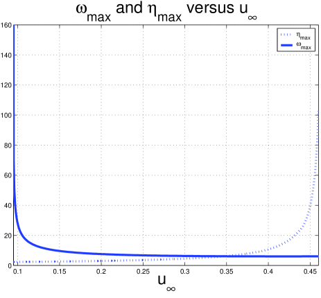
Figure 1: $w_{max}$ and $\eta_{max}$ versus $u_{\infty}$

6.2 Example with Finitely Many Unstable Poles

For the plant (25) and weights $W_{1}(s)=\left(\frac{1+0.1s}{0.4+s}\right)$ and $W_{2}(s)=(0.01s+0.5)$, we find the optimal performance level as $\gamma_{opt}=0.59$. The corresponding optimal ${\cal H}^{\infty}$ controller can be written as (7) which has unstable poles at $0.67\pm 14.09j$, $0.11\pm 28.33j$. Note that all suboptimal ${\cal H}^{\infty}$ controllers for finite dimensional $U$ will have finitely many unstable poles by Corollary 3.3. Therefore we can apply the algorithm in Section 5.

1. Fix $\rho=0.60>\gamma_{opt}=0.59$,

2. The suboptimal controllers can be written as in (10) where $m_{n}$ is given in (6.1) and

   $$E_{\rho} = \frac{0.94+0.35s^{2}}{0.36(0.16-s^{2})},$$

   $$F_{\rho} = \frac{0.36(0.4-s)}{0.0059s^{2}+0.31s+0.35},$$

   $$L_{2} = 0.98s^{3}+2.45s^{2}+1.91s+2.10,$$

   $$L_{1} = s^{3}+1.64s^{2}+0.45s+1.61,$$

   and $U$ is a free parameter such that $U\in{\cal H}^{\infty}$, $\|U\|_{\infty}\leq 1$. We can obtain $P_{1}$ and $P_{2}$ from (5). Note that $P_{1}$ has $\mathbb{C}_{+}$ zeros at $p_{1,2}=0.64\pm 14.064j$, $p_{3,4}=0.081\pm 28.314j$ and $P_{2}$ has $\mathbb{C}_{+}$ zeros at $s_{1,2}=0.29\pm 28.31j$, $s_{3,4}=0.90\pm 14.035j$ and $s_{5}=2.43$. Therefore, the central controller (when $U=0$) for the chosen performance level, $\rho=0.6$, is unstable.

3. Note that $\mathbb{C}_{+}$ zeros of $P_{1}$ and $P_{2}$ are defined in previous step. Then, $\tilde{M}_{d}$ and $\tilde{M}$ can be defined as (19) where $n_{s}=4$ and $n_{p}=5$. By (20), $w_{i}$ and $z_{i}$ can be calculated where conformal mapping parameter, $a$, is chosen as $1$.

4. For all possible integers sets, the minimum $\mu$ resulting in positive semi-definite Pick matrix (21), is $\mu_{opt}=6.15$ in which all integers are equal to $0$.

5. Fix $\mu=100$. The interpolation conditions for $g(z)$ can be written as in (22) where all integers, $n_{i}$, are zero. By the Nevanlinna-Pick interpolation, (see e.g.Foias et al. (1996); Zeren et al. (1998)), $g_{q}(z)$ is obtained. By transformation, $G_{Q}(s)$ can be calculated where $Q(s)$ is a parameterization term such that $Q\in{\cal H}^{\infty}$ and $\|Q\|_{\infty}\leq 1$. We will search for $Q$ satisfying the inequality (23) in the form of $Q(s)=u_{\infty}$ with $|u_{\infty}|\leq 1$. Note that we choose $z_{u}=p_{u}=0$ and all functions in (24) and $P_{1}$, $P_{2}$ are defined before. The search shows that (23) is satisfied for $u_{\infty}\in[0.23,0.33]$. The magnitude of $U(j\omega)$ is shown for $u_{\infty}=0.3$ in Figure 3. Note that $\|U\|_{\infty}\leq 1$. As a result, stable ${\cal H}^{\infty}$ controller achieves the performance level, $\rho=0.6$. By a numerical search, we can find many $u_{\infty}$ values for different $\mu$ resulting in stable ${\cal H}^{\infty}$ controller at $\rho=0.6$ provided that $U$ satisfies the norm condition for chosen $Q=u_{\infty}$. The various $u_{\infty}$ values resulting stable ${\cal H}^{\infty}$ controller can be seen in Figure 3. We observe that as $\mu$ is increased, the range of $u_{\infty}$ stabilizing the controller decreases.

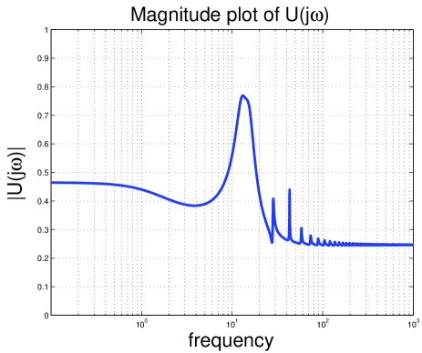
Figure 2: $|U(j\omega)|$ for $\mu=100$ and $u_{\infty}=0.3$

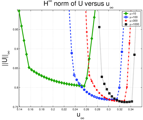
Figure 3: Feasible values of $u_{\infty}$

7 Conclusions

In this paper, stability of ${\cal H}^{\infty}$ controllers are investigated for general time-delay systems. Conditions on the problem data (plant and the weights) are derived that make the optimal and central suboptimal controllers unstable, with finitely or infinitely many $\mathbb{C}_{+}$ poles. A search method is proposed for finding stable suboptimal controllers by properly selecting the free design parameter $U$ appearing in the parameterization of all suboptimal ${\cal H}^{\infty}$ controllers for the class of time delay systems considered. When the optimal and central suboptimal controllers have finitely many $\mathbb{C}_{+}$ poles the search algorithm uses the Nevanlinna-Pick interpolation to derive feasible parameters of the first order $U$. When the optimal and central suboptimal controllers have infinitely many poles in $\mathbb{C}_{+}$, the search algorithm uses a Nyquist argument at each step.

References

- (1)
- Abedor et al. (1989) J.L. Abedor and K. Poolla, “On the strong stabilization of delay system”, Proc. IEEE Conf. on Decision and Control, pp.2317–2318, 1989.
- Barabonov et al. (1996) A.E. Barabanov, “Design of optimal stable controller”, Proc. Conference on Decision and Control, pp.734–738, 1996.
- Zhou et al. (2001) D.U. Campos-Delgado and K. Zhou, “ strong stabilization”, IEEE Transactions on Automatic Control, 46, pp.1968–1972, 2001.
- Campos-Delgado et al. (2003) D.U. Campos-Delgado and K. Zhou, “A parametric optimization approach to and strong stabilizaiton”, Automatica, 39, pp.1205–1211, 2003.
- Choi et al. (2001) Y. Choi and W.K. Chung, “On the stable controller parameterization under sufficient condition”, IEEE Transactions on Automatic Control, 46, pp.1618–1623, 2001.
- Chou et al. (2003) Y.S. Chou, T.Z. Wu and J.L. Leu, “On strong stabilization and strong-stabilization problems”, Proc. Conference on Decision and Control, pp. 5155–5160, 2003.
- Flamm et al. (1987) D.S. Flamm and S.K. Mitter, “ sensitivity minimization for delay systems”, Systems & Control Letters, 9, pp.17–24, 1987 .
- Foias et al. (1996) C. Foias, H. Özbay, and A. Tannenbaum, Robust Control of Infinite Dimensional Systems: Frequency Domain Methods, No.209 in LNCIS, Springer-Verlag, 1996.
- Foias et al. (1986) C. Foias, A. Tannenbaum and G. Zames, “Weighted sensitivity minimization for delay systems”, IEEE Transactions on Automatic Control, 31, pp.763–766, 1986.
- Ganesh et al. (1986) C. Ganesh and J.B. Pearson, “Design of optimal control systems with stable feedback”, Proc. American Control Conference, pp.1969–1973, 1986.
- Gumussoy et al. (2002) S. Gumussoy and H. Özbay, “Control of systems with infinitely many unstable modes and strongly stabilizing controllers achieving a desired sensitivity”, Proc. Mathematical Theory of Networks and Systems, 2002.
- Gumussoy et al. (2004) S. Gumussoy and H. Özbay, “On stable controllers for time-delay systems”, Proc. of the 16th Mathematical Theory of Network and Systems, 2004.