A novel class of translationally invariant
spin chains with long-range interactions

Abstract

We introduce a new class of open, translationally invariant spin chains with long-range interactions depending on both spin permutation and (polarized) spin reversal operators, which includes the Haldane–Shastry chain as a particular degenerate case. The new class is characterized by the fact that the Hamiltonian is invariant under “twisted” translations, combining an ordinary translation with a spin flip at one end of the chain. It includes a remarkable model with elliptic spin-spin interactions, smoothly interpolating between the XXX Heisenberg model with anti-periodic boundary conditions and a new open chain with sites uniformly spaced on a half-circle and interactions inversely proportional to the square of the distance between the spins. We are able to compute in closed form the partition function of the latter chain, thereby obtaining a complete description of its spectrum in terms of a pair of independent $\mathrm{su}(1|1)$ and $\mathrm{su}(m/2)$ motifs when the number $m$ of internal degrees of freedom is even. This implies that the even $m$ model is invariant under the direct sum of the Yangians $Y(\mathrm{gl}(1|1))$ and $Y(\mathrm{gl}(0|m/2))$. We also analyze several statistical properties of the new chain’s spectrum. In particular, we show that it is highly degenerate, which strongly suggests the existence of an underlying (twisted) Yangian symmetry also for odd $m$.

1 Introduction

Exactly solvable quantum dynamical models in one dimension and spin chains with long-range interactions have given rise to interesting applications as prototypes of strongly correlated systems exhibiting generalized exclusion statistics Ha91b ; HHTBP92 ; GS05 ; Gr09 , as well as in connection with such diverse phenomena as the quantum Hall effect AI94 ; BK09 , quantum transport in mesoscopic systems BR94 ; Ca95 or quantum simulation of long-range magnetism HGCK16 . Moreover, recent experiments involving optical lattices of ultracold Rydberg atoms and trapped ions have opened up the exciting possibility of experimentally probing various properties of such low-dimensional quantum spin chains in a very precise way PC04 ; GL14 ; KCIKD09 ; RGLSS14 ; JLHHZ14 ; SZFHC15 . In the context of high-energy physics, quantum spin chains with long-range interactions have played a key role in the computation of the spectrum of the dilation operator in $N=4$ super Yang–Mills theories MZ03 ; SS04 ; Be12 . Intriguing connections between (1+1)-dimensional conformal field theory (CFT) and exactly solvable models with long-range interactions have also been uncovered in recent years CS10 ; NCS11 ; BQ14 ; TNS14 . In the same vein, it has been found that the Casimir equation for conformal blocks in $d$ dimensions can be transformed into the eigenvalue problem for a hyperbolic Calogero–Sutherland model associated with the $BC_{N}$ reflection group IS16 ; ILLS18 .

The translationally invariant Haldane–Shastry (HS) spin-$\frac{1}{2}$ chain Ha88 ; Sh88 , whose spins are uniformly spaced on a circular lattice and exhibit two-body interactions inversely proportional to the square of their chord distances, is the prototypical example of an exactly solvable lattice model with long-range interactions. The HS spin chain features many interesting properties, a few of which we shall briefly review next. Indeed, its exact ground state coincides with the $U\to\infty$ limit of Gutzwiller’s variational wavefunction for the Hubbard model, and with the one-dimensional version of Anderson’s “resonating-valence-bond state” An73 ; FA74 ; ABZH87 ; Ha88 . Moreover, its spinon excitations Ha91 (in the antiferromagnetic case) can be described through a generalized Pauli exclusion principle, as they can be regarded as anyons with exclusion parameter $g=1/2$ (so called semions) Ha91b . The original —$\mathrm{su}(2)$— HS spin chain and its $\mathrm{su}(m)$ generalization also exhibit Yangian quantum group symmetry, even for a finite number of lattice sites HHTBP92 ; BGHP93 . As a consequence, the spectrum of these integrable spin chains can be described by means of finite sequences of the binary digits 0 and 1, known as “motifs” in the literature HHTBP92 , related to certain finite-dimensional representations of the Yangian algebra KKN97 ; NT98 . In addition, the complete energy spectrum of these chains, including the degeneracy of each level, can be generated from the energy function of an associated one-dimensional classical vertex model BBH10 . The $\mathrm{su}(m)$ HS chain can also be obtained by taking the freezing limit Po93 of the $\mathrm{su}(m)$ spin Sutherland model HH92 , whose particles possess both dynamical and spin degrees of freedom. More precisely, in the large coupling constant limit the spin part of the latter model’s Hamiltonian decouples from the dynamical one and yields the Hamiltonian of the HS chain. In fact, the partition function of the $\mathrm{su}(m)$ HS chain can be computed in closed form FG05 by taking advantage of this decoupling of the spin and dynamical degrees of freedom of the spin Sutherland model, which is the essence of Polychronakos’s freezing trick.

In view of these remarkable properties, several methods have been proposed for constructing integrable or exactly solvable variants of the HS chain. In particular, the connection between quantum integrable models with long-range interactions and different (extended) root systems has proved a useful tool in this endeavor OP83 ; CS02 . The main idea in this respect is to replace the $A_{N-1}$ root system associated with the interaction potential of the spin Sutherland model, which yields the original HS chain, by other (extended) root systems like, e.g., $BC_{N}$, $B_{N}$ and $D_{N}$. The spin Sutherland models associated with all of these root systems have in fact been studied in the literature, and used to construct spin chains of HS type by taking their strong coupling limits BPS95 ; EFGR05 ; BFG11 ; BFG13 . In particular, the exact partition function of each of these chains has been computed in closed form applying the freezing trick to their parent spin dynamical models. It should be noted, however, that none of these integrable variants of the HS chain retains the translational invariance characteristic of the original model.

Several extensions of the HS spin chain with lattice sites arbitrarily distributed on a circle and exact ground state wavefunctions have also been recently constructed using infinite matrix product states (MPSs) CS10 related to certain rational CFTs. More precisely, it has been observed that the correlators associated with the chiral vertex operators of such CFTs play the role of infinite MPSs yielding the ground state wavefunctions of these HS-like chains CS10 ; NCS11 ; BQ14 ; TNS14 . Using the null field techniques related to rational CFTs, one can explicitly construct the Hamiltonians of these models and study interesting physical properties thereof, like, e.g., the spin-spin correlation functions. However, these models lack two of the key properties of the original HS chain, namely, they do not exhibit translational invariance nor are they integrable in general. More recently, exact ground state wavefunctions of some HS-like spin chains, with open boundary conditions and lattice points arbitrarily distributed on a half-circle, have been constructed using infinite MPSs related to suitable boundary CFTs and corresponding null fields TS15 . Again, these CFT-inspired generalizations of the HS chain with open boundary conditions become integrable TS15 and, in fact, exactly solvable BFG16 , only for some special choices of the lattice points, but none of them possess the translational invariance of the original HS chain.

In this work we construct a new solvable spin chain with inverse-square long-range interactions possessing two of the essential properties of the $\mathrm{su}(m)$ HS chain, namely translational invariance and uniform spacing of the sites. Our construction is still based on applying Polychronakos’s freezing trick to an appropriate (solvable) translationally invariant spin dynamical model FGGRZ01 . However, unlike the original HS chain and its $BC_{N}$, $B_{N}$ and $D_{N}$ versions mentioned above, neither this dynamical model nor the resulting chain are associated with an extended root system in the standard fashion. More precisely, the spin chain we shall construct is translationally invariant, in the sense that (like the original HS chain of $A_{N-1}$ type) the interactions between sites $i$ and $j$ depends only on the difference $i-j$. However, in contrast with the latter chain, its Hamiltonian includes both spin permutation and spin flip operators generating the full Weyl group of $D_{N}$ type. In particular, the presence of the spin flip operators in the Hamiltonian also distinguishes the new model from the spin chains constructed from infinite MPSs in the above cited references. On the other hand, we shall see that the new chain’s sites are uniformly arranged on a half-circle, like in uniformly spaced HS chains of $BC_{N}$ type, so that the model is naturally regarded as an open chain. As such, the usual translation operator does not commute with the Hamiltonian due to boundary terms. Remarkably, however, the new model is exactly invariant under a cyclic group of “twisted” translations, suitably combining standard translations with spin flips. This symmetry is indeed one of the hallmarks of the model, which we believe sets it apart from all the solvable spin chains with long-range interactions discussed above.

In fact, our construction can be substantially extended in two different directions. In the first place, we can replace the standard spin flip operators in the Hamiltonian by partially polarized versions thereof without compromising any of the key properties discussed above, namely translational invariance of the interactions, uniform spacing of the sites, symmetry under twisted translations and solvability. Secondly, we can allow for much more general spin-spin interactions such that the resulting models still possess the characteristic symmetry under twisted translations discussed above. This yields a wide class of new open, translationally invariant spin chains with long-range interactions and uniformly spaced sites, whose solvability properties are certainly worth investigating. This class includes a remarkable model with elliptic interactions, reminiscent of the well known Inozemtsev In90 chain, which smoothly interpolates between the new solvable model with inverse-square interactions and the twisted $\mathrm{su}(m)$ XXX Heisenberg model ABB88 ; Ni13 ; Ga14 ; NW14 .

We shall study in detail the solvable model with inverse square interactions and ordinary (minimally polarized) spin flip operators mentioned above, which formally reduces to the HS chain if the latter operators are replaced by the identity. Taking advantage of the connection between this chain and its associated spin dynamical model, we shall evaluate the chain’s partition function in closed form. As it turns out, the structure of this partition function depends critically on the parity of the number $m$ of spin degrees of freedom. In particular, for even $m$ the partition function factorizes as the product of the partition functions of the (antiferromagnetic) $\mathrm{su}(m/2)$ and $\mathrm{su}(1|1)$-supersymmetric HS chains. This fact is certainly surprising, since the new model is built from standard (non-supersymmetric) permutation operators, and deserves further study. On a more concrete level, the formula for the partition function in the even $m$ case straightforwardly yields a complete description of the spectrum, including the precise degeneracy of each level, in terms of pairs of $\mathrm{su}(1|1)$ and $\mathrm{su}(m/2)$ motifs, and establishes the invariance of the model under the direct sum of the Yangians $Y(\mathrm{gl}(1|1))$ and $Y(\mathrm{gl}(0|m/2))$.

The paper’s organization is as follows. The new class of models is introduced in section 2, where we also discuss their characteristic invariance under twisted translations. In section 3 we show how these models arise from a suitable spin dynamical model of Calogero–Sutherland type through Polychronakos’s freezing trick. Using this fact, in section 4 we derive an exact closed-form expression for the partition function of the novel spin chain with inverse-square interactions. This expression is used in section 5 to derive a motif-based description of the spectrum of the latter chain in the even $m$ case. Section 6 contains a brief discussion of some statistical properties of the spectrum of this model, in comparison with related models like the $A_{N-1}$ and $D_{N}$ HS chains. In section 7 we present our conclusions, and briefly discuss several avenues for further research suggested by our results. The paper ends with four technical appendices in which we describe in detail the derivation of the spectrum of the spin dynamical model associated with the new solvable chain, evaluate a sum used in section 4 to determine its partition function, and compute the standard deviation of its spectrum in closed form.

2 The models

In this paper we introduce a remarkable new class of $\mathrm{su}(m)$ spin chains with long-range interactions. We shall start by discussing the simplest representative of the latter class, with Hamiltonian

$${\mathcal{H}}=\frac{1}{4}\sum_{1\leqslant i<j\leqslant N}\bigg{[}\frac{1+S_{ij}}{\sin^{2}(\theta_{i}-\theta_{j})}+\frac{1+\widetilde{S}_{ij}}{\cos^{2}(\theta_{i}-\theta_{j})}\bigg{]}\,,\qquad\theta_{k}:=\frac{k\pi}{2N}\,,$$ (1)

where $S_{ij}$ is the operator permuting the $i$-th and $j$-th spins, $\widetilde{S}_{ij}=S_{ij}S_{i}S_{j}$, and $S_{k}$ is a local operator at site $k$ satisfying $S_{k}^{2}=1$ for all $k$. More precisely, if we label the $\mathrm{su}(m)$ internal degrees of freedom by the half-integers $-M,-M+1,\dots,M:=(m-1)/2$, the action of the operator $S_{ij}$ on the canonical basis states

$$|s_{1},\dots,s_{N}\rangle=:|\mathbf{s}\rangle\,,\qquad s_{k}\in\{-M,-M+1,\dots,M\}\,,$$

of the internal (spin) Hilbert space $\Sigma:=\bigotimes\limits_{i=1}^{N}{\mathbb{C}}^{m}$ is given by

$$S_{ij}|s_{1},\dots,s_{i},\dots,s_{j},\dots,s_{N}\rangle=|s_{1},\dots,s_{j},\dots,s_{i},\dots,s_{N}\rangle\,.$$

The operators $S_{ij}$ and $S_{i}S_{j}$ (with $1\leqslant i<j\leqslant N$) generate the Weyl group of the $D_{N}$ classical root system, algebraically determined by the non-trivial relations

$$S_{ij}^{2}=(S_{i}S_{j})^{2}=1,\qquad S_{ij}S_{jk}=S_{ik}S_{ij}=S_{jk}S_{ik},\qquad S_{ij}S_{i}S_{k}=S_{j}S_{k}S_{ij}\,,$$

where the indices $i,j,k$ are all distinct and it is understood that $S_{ij}=S_{ji}$, for $i>j$. The model (1), however, does not have the standard form

$${\mathcal{H}}_{D}=\sum_{i<j}\Big{[}f(\xi_{i}-\xi_{j})(1+S_{ij})+f(\xi_{i}+\xi_{j})(1+\widetilde{S}_{ij})\Big{]}$$ (2)

of a spin chain with sites $\xi_{k}$ associated with the $D_{N}$ root system BFG09 ; BFG11 . Nor is it clearly associated with the $A_{N}$ root system like, e.g., the original HS chain and its rational Fr93 ; Po93 , hyperbolic FI94 and elliptic In90 counterparts, due to the presence of the operators $S_{i}$ in the Hamiltonian. Thus the chain Hamiltonian (1) is not directly associated with an extended root system, unlike most chains of HS type considered so far in the literature (see, e.g., Ya95 ; BPS95 ; BFG11 ; BFG13 for other instances of HS-like chains of $BC_{N}$, $B_{N}$ and $D_{N}$ types).

For each $k=1,\dots,N$ the operator $S_{k}$ generates the cyclic group $Z_{2}$ of order $2$, which has two inequivalent irreducible representations (necessarily one-dimensional, as $Z_{2}$ is abelian) $R_{\pm}$ for which $S_{k}=\pm 1$. If the internal space ${\mathbb{C}}^{m}$ decomposes under the action of each operator $S_{k}$ as ${\mathbb{C}}^{m}=R_{+}^{l}\oplus R_{-}^{m-l}$, we shall say that the degree of polarization of the corresponding $m$-dimensional representation of $Z_{2}$ is $d=|2l-m|\in\{\varepsilon,\varepsilon+2,\dots,m\}$ (where $\varepsilon\in\{0,1\}$ is the parity of $m$). When $d=m$ is maximal, i.e., when $S_{k}$ is either $1$ or $-1$ for all $k$, $\widetilde{S}_{ij}=S_{ij}$ and consequently the Hamiltonian (1) reduces to the Hamiltonian ${\mathcal{H}}_{\mathrm{HS}}$ of the HS spin chain

$${\mathcal{H}}_{\mathrm{HS}}=\frac{J}{2}\sum_{i<j}\frac{1+S_{ij}}{\sin^{2}\Bigl{(}\tfrac{\pi(i-j)}{N}\Bigr{)}}$$ (3)

with $J=2$. Thus the model (1) can be formally regarded as an extension of the Haldane–Shastry spin chain. On the other hand, in the remaining cases where the polarization is not maximal (i.e., for $d<m$), the spin-spin interactions associated with the operators $S_{ij}$ and $\tilde{S}_{ij}$ do not coincide with each other. As a result, the Hamiltonian (1) describes a novel class of spin chains with uniformly spaced sites (in fact, we shall see that the sites are arranged on the upper half of a circle). In this paper we shall focus on the simplest case, with minimal polarization $d=\varepsilon$. It is then convenient to decompose ${\mathbb{C}}^{m}$ into $(m-\varepsilon)/2$ copies of the two-dimensional (reducible) representation $R_{+}\oplus R_{-}$ plus $\varepsilon$ copies of $R_{\pm}$. We shall choose the canonical spin basis so that each space $R_{+}\oplus R_{-}$ is spanned by the basis vectors $\{|-i\rangle,|i\rangle\}$ with $i=1,\dots,M$, so that for $\varepsilon=1$ (i.e., if $m$ is odd) the remaining one-dimensional space $R_{\pm}$ is spanned by $|0\rangle$. A moment’s thought reveals that we can also choose the basis so that $S_{k}|i\rangle=|-i\rangle$ for $i=1,\dots,M$ and (if $\varepsilon=1$) $S_{k}|0\rangle=|0\rangle$. Thus in this case $S_{k}$ acts on the internal space as a spin flip operator:

$$S_{k}|\mathbf{s}\rangle=|s_{1},\dots,-s_{k},\dots,s_{N}\rangle\,.$$

Except in the trivial case with maximum polarization $d=m$, the two different spin-spin interactions in the Hamiltonian (1) can be regarded as inverse square interactions between two spins or one spin and its image, as we shall now explain. Indeed, the first term in eq. (1) can be interpreted as a two-body interaction with strength inversely proportional to the square of the chord distance between the $i$-th and $j$-th spins, provided that the chain sites $\xi_{k}$ are located at the points $\xi_{k}=\mathrm{e}^{2\mathrm{i}\theta_{k}}$ in the complex plane. Since $\theta_{k}=(k\pi)/(2N)$ with $k=1,\dots,N$, the chain sites lie on uniformly spaced points in the unit upper half-circle $|z|=1$, $\operatorname{Im}z\geqslant 0$, with angular coordinates $\arg\xi_{k}=2\theta_{k}$. Thus it is natural to regard the model (1) as an open chain, in spite of its translationally invariant interactions. If we now define the image $\xi_{k}^{*}$ of the chain site $\xi_{k}$ as its reflection with respect to the origin, i.e., $\xi_{k}^{*}=-\xi_{k}$, we have

$$\big{|}\xi_{k}-\xi_{j}^{*}\big{|}=\big{|}\mathrm{e}^{2\mathrm{i}\theta_{k}}+\mathrm{e}^{2\mathrm{i}\theta_{j}}\big{|}=2\cos(\theta_{j}-\theta_{k}).$$

Thus the second term in the Hamiltonian (1) can be interpreted as a two-body interaction of each spin in the chain with the image of any other spin, whose strength is again inversely proportional to the square of their distance.

We shall next discuss the remarkable behavior of the Hamiltonian (1) under translations along the chain sites, which, as mentioned in the Introduction, is one of the model’s distinctive features. To this end, let $T$ denote the left translation operator defined by

$$T|s_{1},\dots,s_{N}\rangle:=|s_{2},\dots,s_{N},s_{1}\rangle\,,$$

so that $T^{\dagger}=T^{-1}$ and

$$T^{\dagger}S_{ij}T=S_{i+1,j+1},\qquad T^{\dagger}\widetilde{S}_{ij}T=\widetilde{S}_{i+1,j+1}$$

with

$$S_{k,N+1}\equiv S_{1k}\,,\qquad\widetilde{S}_{k,N+1}\equiv\widetilde{S}_{1k}\,.$$ (4)

Since the interaction strength between sites $i$ and $j$ in the Hamiltonian (1) depends only on $i-j$, it may naively seem that ${\mathcal{H}}$ commutes with the translations generator $T$ when we use eqs. (4) to deal with boundary terms. This is actually not the case due to the open nature of the model (except, of course, in the trivial case $d=m$), which is also apparent from the fact that the interaction strengths of site $1$ with sites $2$ and $N$ differ. More precisely, taking eq. (4) into account we obtain

$$T^{\dagger}{\mathcal{H}}T =\frac{1}{4}\sum_{1\leqslant i<j\leqslant N}\bigg{[}\frac{1+S_{i+1,j+1}}{\sin^{2}(\theta_{i}-\theta_{j})}+\frac{1+\widetilde{S}_{i+1,j+1}}{\cos^{2}(\theta_{i}-\theta_{j})}\bigg{]}=\frac{1}{4}\sum_{2\leqslant i<j\leqslant N}\bigg{[}\frac{1+S_{i,j}}{\sin^{2}(\theta_{i}-\theta_{j})}+\frac{1+\widetilde{S}_{i,j}}{\cos^{2}(\theta_{i}-\theta_{j})}\bigg{]}$$

$$+\frac{1}{4}\sum_{j=2}^{N}\bigg{[}\frac{1}{\sin^{2}(\theta_{j}-\theta_{1})}+\frac{1}{\cos^{2}(\theta_{j}-\theta_{1})}+\frac{S_{1j}}{\sin^{2}(\theta_{j-1}-\theta_{N})}+\frac{\widetilde{S}_{1j}}{\cos^{2}(\theta_{j-1}-\theta_{N})}\bigg{]}\,.$$

From the identities

$$\sin^{2}(\theta_{j-1}-\theta_{N})=\sin^{2}\bigl{(}\tfrac{\pi(j-1-N)}{2N}\bigr{)}=\cos^{2}\bigl{(}\tfrac{\pi(j-1)}{2N}\bigr{)}\equiv\cos^{2}(\theta_{j}-\theta_{1}),$$

and similarly $\cos^{2}(\theta_{j-1}-\theta_{N})=\sin^{2}(\theta_{j}-\theta_{1})$, it then follows that

$$T^{\dagger}{\mathcal{H}}T =\frac{1}{4}\sum_{2\leqslant i<j\leqslant N}\bigg{[}\frac{1+S_{ij}}{\sin^{2}(\theta_{i}-\theta_{j})}+\frac{1+\widetilde{S}_{ij}}{\cos^{2}(\theta_{i}-\theta_{j})}\bigg{]}+\frac{1}{4}\sum_{j=2}^{N}\bigg{[}\frac{1+S_{1j}}{\cos^{2}(\theta_{j}-\theta_{1})}+\frac{1+\widetilde{S}_{1j}}{\sin^{2}(\theta_{j}-\theta_{1})}\bigg{]}$$

$$={\mathcal{H}}-\sum_{j=2}^{N}\frac{\cos\bigl{(}2(\theta_{j}-\theta_{1})\bigr{)}}{\sin^{2}\bigl{(}2(\theta_{j}-\theta_{1})\bigr{)}}\,S_{1j}(1-S_{1}S_{j})\,.$$

Thus ${\mathcal{H}}$ does not commute with the left translation $T$ unless $S_{j}=\pm 1$ for all $j$, i.e., in the trivial case of maximal polarization when the model (1) reduces to the HS spin chain. However, this problem is easily cured introducing the “twisted” (left) translation operator

$${\mathcal{T}}:=TS_{1}\,.$$

Indeed, taking into account that

$${\mathcal{T}}^{\dagger}S_{ij}{\mathcal{T}}=S_{1}T^{\dagger}S_{ij}TS_{1}=S_{1}S_{i+1,j+1}S_{1}=\begin{cases}S_{i+1,j+1}\,,&j<N\\ S_{1}S_{1,i+1}S_{1}=S_{1}S_{i+1}S_{1,i+1}=\widetilde{S}_{1,i+1}\,,&j=N\,,\end{cases}$$

and similarly for ${\mathcal{T}}^{\dagger}\widetilde{S}_{ij}{\mathcal{T}}$ (since $S_{i+1,j+1}$ or $\widetilde{S}_{i+1,j+1}$ commutes with $S_{1}$ unless $j=N$) and proceeding as above we obtain

$${\mathcal{T}}^{\dagger}{\mathcal{H}}{\mathcal{T}}= \frac{1}{4}\sum_{2\leqslant i<j\leqslant N}\bigg{[}\frac{1+S_{ij}}{\sin^{2}(\theta_{i}-\theta_{j})}+\frac{1+\widetilde{S}_{ij}}{\cos^{2}(\theta_{i}-\theta_{j})}\bigg{]}$$

$$+\frac{1}{4}\sum_{j=2}^{N}\bigg{[}\frac{1}{\sin^{2}(\theta_{j}-\theta_{1})}+\frac{1}{\cos^{2}(\theta_{j}-\theta_{1})}+\frac{\widetilde{S}_{1j}}{\sin^{2}(\theta_{j-1}-\theta_{N})}+\frac{S_{1j}}{\cos^{2}(\theta_{j-1}-\theta_{N})}\bigg{]}={\mathcal{H}}\,.$$

We thus see that the chain Hamiltonian (1) commutes with the elements of the group of twisted translations generated by ${\mathcal{T}}$. Since $S_{i}T=TS_{i+1}$ we have ${\mathcal{T}}^{k}=T^{k}S_{k}\cdots S_{1},$ and hence

$${\mathcal{T}}^{N}=S_{N}\cdots S_{1}\,.$$

It follows that ${\mathcal{T}}^{2N}=1$, so that the latter group is a cyclic group of order $2N$ (i.e., twice that of the group of standard translations). Of course, for $d=m$ (i.e, when the model (1) reduces to the HS chain), and only in this case, the twisted translation operator reduces to the standard one $T$. This again underscores the fundamentally new character of the model (1) in the case of non-maximal polarization $d<m$. In particular, in the case of minimal polarization $d=\varepsilon$ the operator ${\mathcal{T}}$ acts on the canonical spin basis as

$${\mathcal{T}}|s_{1},\dots,s_{N}\rangle=|s_{2},\dots,s_{N},-s_{1}\rangle\,.$$

Thus in this case, which shall be extensively dealt with in the remaining sections, the twisted translation consists of a translation followed by a flip of the last site’s spin.

Remark 1.

The twisted translation operator ${\mathcal{T}}$ satisfies the identities

$${\mathcal{T}}^{\dagger}S_{ij}{\mathcal{T}}=S_{i+1,j+1},\qquad{\mathcal{T}}^{\dagger}\widetilde{S}_{ij}{\mathcal{T}}=\widetilde{S}_{i+1,j+1}$$

provided that we identify $S_{k,N+1}$ with $\widetilde{S}_{1k}$ and $\widetilde{S}_{k,N+1}$ with $S_{1k}$, which is akin to using twisted boundary conditions. Note, however, that we have not used twisted boundary conditions (or, indeed, boundary conditions of any kind) in the definition of the model (1), since its Hamiltonian contains only operators with indices in the range $1,\dots,N$. In particular, the new model is not a variant of the twisted HS chain introduced by Fukui and Kawakami FK96 . Indeed, after a gauge transformation of the original spin operators the Hamiltonian of the latter model describes a translationally invariant chain with sites uniformly arranged on a circle and periodic boundary conditions, differing from the original HS chain only in the strength of the spin-spin interactions.

In fact, there is a much wider class of models sharing with the chain (1) its symmetry under twisted translations. To see this, consider the Hamiltonian

$${\mathcal{H}}=\sum_{1\leqslant i<j\leqslant N}\big{[}f(i-j)(1+S_{ij})+\widetilde{f}(i-j)(1+\widetilde{S}_{ij})\big{]}\,,$$

where $f$ is an even function of one variable. A straightforward computation along the previous lines leads to the identity

$${\mathcal{T}}^{\dagger}{\mathcal{H}}{\mathcal{T}}= \sum_{2\leqslant i<j\leqslant N}\big{[}f(i-j)(1+S_{ij})+\widetilde{f}(i-j)(1+\widetilde{S}_{ij})\big{]}$$

$$+\sum_{j=2}^{N}\big{[}f(j-1-N)(1+\widetilde{S}_{1,j})+\widetilde{f}(j-1-N)(1+S_{1j})\big{]}\,.$$

We thus see that ${\mathcal{H}}$ will commute with ${\mathcal{T}}$ provided that the following two identities between the unknown functions $f$ and $\widetilde{f}$ are satisfied:

$$\widetilde{f}(x)=f(x-N)\,,\qquad f(x)=\widetilde{f}(x-N)\,.$$

The first identity relates $\widetilde{f}$ to $f$, while the second one is then equivalent to the condition that $f$ be $2N$-periodic. These considerations lead to the Hamiltonian

$${\mathcal{H}}=\sum_{1\leqslant i<j\leqslant N}\big{[}f(i-j)(1+S_{ij})+f(i-j-N)(1+\widetilde{S}_{ij})\big{]}\,,$$ (5)

with $f$ an even $2N$-periodic function. This periodicity condition makes it natural to regard the latter model as a uniformly spaced semi-circular (open) chain, with sites $\xi_{k}=\mathrm{e}^{\mathrm{i}k\pi/N}\equiv\mathrm{e}^{2\mathrm{i}\theta_{k}}$. The model (1) is then obtained requiring that $f(i-j)$ be the square of the inverse distance between sites $i$ and $j$.

Remark 2.

The new chain (1) is also related to the (non-translationally invariant) HS chain of $D_{N}$ type. To see this, note first of all that the Hamiltonian (1) can be written as

$${\mathcal{H}}=\sum_{1\leqslant i<j\leqslant N}\bigg{(}\frac{1+S_{ij}}{|\xi_{i}-\xi_{j}|^{2}}+\frac{1+\widetilde{S}_{ij}}{|\xi_{i}-\xi_{j}^{*}|^{2}}\bigg{)}\,,$$ (6)

where the chain sites $\xi_{k}=\mathrm{e}^{2\mathrm{i}\theta_{k}}=-\xi_{k}^{*}$ are the coordinates of the unique (up to an overall translation) equilibrium of the potential

$$U(\mathbf{x})=\sum_{1\leqslant i<j\leqslant N}\bigg{(}\frac{1}{|z_{i}-z_{j}|^{2}}+\frac{1}{|z_{i}-z_{j}^{*}|^{2}}\bigg{)},$$ (7)

with $z_{k}=-z_{k}^{*}=\mathrm{e}^{2\mathrm{i}x_{k}}$ in the set $x_{1}<\cdots<x_{N}<x_{1}+\pi/2$. If, on the other hand, we define the image $\xi_{k}^{*}$ by $\xi_{k}^{*}=\overline{\xi_{k}}$ (where the bar denotes complex conjugation), then

$$\big{|}\xi_{k}-\xi_{j}^{*}\big{|}=\big{|}\mathrm{e}^{2\mathrm{i}\theta_{k}}-\mathrm{e}^{-2\mathrm{i}\theta_{j}}\big{|}=2\big{|}\sin(\theta_{j}+\theta_{k})\big{|}\,.$$

Taking $\theta_{k}$ as the coordinates of the unique equilibrium (in the set $|x_{1}|<x_{2}<\cdots<x_{N}<\pi-x_{N-1}$) of the potential (7) with $z_{j}^{*}=\overline{z_{j}\vrule width=0.0pt,height=6.0pt}$, the resulting Hamiltonian (6) with $\xi_{k}^{*}=\overline{\xi_{k}}$ becomes that of the HS chain of $D_{N}$ type

$${\mathcal{H}}_{\text{HS,D}}=\frac{J}{2}\sum_{i<j}\left[\frac{1+S_{ij}}{\sin^{2}(\theta_{i}-\theta_{j})}+\frac{1+\widetilde{S}_{ij}}{\sin^{2}(\theta_{i}+\theta_{j})}\right]$$ (8)

with $J=1/2$.

3 Spin dynamical model

As mentioned above, from now on we shall deal exclusively with the case of minimal polarization $d=\varepsilon$, when the operators $S_{i}$ act simply as ordinary spin flip operators. One of the main aims of this paper is to derive a closed-form expression for the partition function of the Hamiltonian (1) by exploiting its connection with a non-standard spin dynamical model introduced in ref. FGGRZ01b . The existence of such an expression shows that the model (1) is a simple but non-trivial example of an exactly solvable spin chain with long-range two-body interactions and twisted translation invariance. Note in this respect that the rational and hyperbolic chains of HS type mentioned above are solvable but not translationally invariant, while the Inozemtsev chain In90 (an HS-like spin chain with elliptic two-body interactions) is translationally invariant but not solvable.

More precisely, the solvability of the spin chain (1) relies on its connection with the solvable spin dynamical model with Hamiltonian

$$H =-\Delta+8a\sum_{1\leqslant i<j\leqslant N}\bigg{(}\frac{a+S_{ij}}{|z_{i}-z_{j}|^{2}}+\frac{a+\widetilde{S}_{ij}}{|z_{i}-z_{j}^{*}|^{2}}\bigg{)}$$

$$=-\Delta+2a\sum_{i<j}\bigg{[}\frac{a+S_{ij}}{\sin^{2}(x_{i}-x_{j})}+\frac{a+\widetilde{S}_{ij}}{\cos^{2}(x_{i}-x_{j})}\bigg{]}\,,\qquad z_{k}=-z_{k}^{*}:=\mathrm{e}^{2\mathrm{i}x_{k}}\,,$$ (9)

where $\Delta:=\sum_{i}\frac{\partial^{2}}{\partial x_{i}^{2}}$ and $a>1/2$. The key idea, which is originally due to Polychronakos Po94 , is to take the large coupling constant limit $a\to\infty$ in eq. (9). In this limit the eigenfunctions of $H$ become sharply peaked around the coordinates of the equilibrium position of the scalar potential (7), explicitly given by

$$U(\mathbf{x})=\sum_{1\leqslant i<j\leqslant N}\bigg{(}\frac{1}{|z_{i}-z_{j}|^{2}}+\frac{1}{|z_{i}-z_{j}^{*}|^{2}}\bigg{)}=\sum_{i<j}\sin^{-2}\bigl{(}2(x_{i}-x_{j})\bigr{)}\,,$$

in the configuration space $A$ of the model (9). Note that this configuration space can be taken as

$$A=\Big{\{}\mathbf{x}:=(x_{1},\dots,x_{N})\in{\mathbb{R}}^{N}:x_{1}<x_{2}\dots<x_{N}<x_{1}+\tfrac{\pi}{2}\Big{\}}\,,$$ (10)

due to the impenetrable nature of the singularities of the scalar potential (7) on the hyperplanes $x_{i}-x_{j}=k\pi,(2k+1)\pi/2$ with $k\in{\mathbb{Z}}$. The unique global minimum of $U$ in the open set $A$ is the point whose coordinates $x_{k}=k\pi/(2N)\equiv\theta_{k}$ coincide with the sites of the chain (1), apart from an irrelevant overall translation FG14 . Thus in the limit $a\to\infty$ the particles’ dynamic and spin degrees of freedom effectively decouple. In fact, since

$$H=H_{\mathrm{sc}}+8aH_{\mathrm{spin}}(\mathbf{x})$$

with

$$H_{\mathrm{sc}} :=-\Delta+8a(a-1)\sum_{i<j}\sin^{-2}\bigl{(}2(x_{i}-x_{j})\bigr{)},$$ (11)

$$H_{\mathrm{spin}}(\mathbf{x}) :=\frac{1}{4}\sum_{i<j}\bigg{[}\frac{1+S_{ij}}{\sin^{2}(x_{i}-x_{j})}+\frac{1+\widetilde{S}_{ij}}{\cos^{2}(x_{i}-x_{j})}\bigg{]}$$ (12)

and $H_{\mathrm{spin}}(\theta_{1},\dots,\theta_{N})={\mathcal{H}}$, for $a\to\infty$ the energies of the spin dynamical model (9) are approximately given by

$$E_{ij}\simeq E_{i}+8a{\mathcal{E}}_{j}\,,$$

where $E_{i}$ and ${\mathcal{E}}_{j}$ respectively denote two arbitrary eigenvalues of $H_{\mathrm{sc}}$ and ${\mathcal{H}}$. From the above relation we immediately obtain the following exact formula for the partition function ${\mathcal{Z}}$ of the chain (1):

$${\mathcal{Z}}(T)=\lim_{a\to\infty}\frac{Z(8aT)}{Z_{\mathrm{sc}}(8aT)}\,,$$ (13)

where $Z$ and $Z_{\mathrm{sc}}$ are respectively the partition functions of the Hamiltonians $H$ and $H_{\mathrm{sc}}$.

In fact, the general spin chain Hamiltonian (5) can also be derived from a spin dynamical model akin to eq. (9). Indeed, let

$$H=-\Delta+2a\sum_{i<j}\big{[}F(x_{i}-x_{j})(a+S_{ij})+F(x_{i}-x_{j}-\tau)(a+\widetilde{S}_{ij})]\,,$$ (14)

where $F(x)$ is an even $2\tau$-periodic function. The spin chain Hamiltonian constructed from $H$ applying the freezing trick discussed above is given (up to a proportionality factor which can be chosen at will) by

$${\mathcal{H}}=\sum_{i<j}\big{[}F(\xi_{j}-\xi_{i})(1+S_{ij})+F(\xi_{j}-\xi_{i}-\tau)(1+\widetilde{S}_{ij})]\,,$$ (15)

where $(\xi_{1},\dots,\xi_{N})=:\boldsymbol{\xi}$ are the coordinates of the equilibrium of the scalar potential

$$U(\mathbf{x})=\sum_{i<j}u(x_{i}-x_{j})\,,\qquad u(x):=F(x)+F(x-\tau)\,,$$

in the region $\{\mathbf{x}\in{\mathbb{R}}^{N}:x_{1}<\cdots<x_{N}<x_{1}+\tau\}$. To see that $\boldsymbol{\xi}$ is uniquely defined (up to a rigid translation), note first of all that $u$ is even and $\tau$-periodic. Indeed,

$$\left\{\begin{aligned} u(-x)&=F(-x)+F(-x-\tau)=F(x)+F(x+\tau)=F(x)+F(x-\tau)\equiv u(x)\,,\\ u(x+\tau)&=F(x+\tau)+F(x)=F(x-\tau)+F(x)\equiv u(x)\,.\end{aligned}\right.$$

It then follows that $u^{\prime}$ is odd and $\tau$-periodic. Furthermore, $u^{\prime}(\tau/2)=0$, since

$$u^{\prime}(x+\tau)=u^{\prime}(x)\implies u^{\prime}(\tau/2)=u^{\prime}(-\tau/2)=-u^{\prime}(\tau/2)\,.$$

Reasoning as in Theorems 1-2 of ref. FG14 we conclude that

$$\xi_{k}=\frac{k\tau}{N}\,,\qquad k=1,\dots,N\,,$$

provided that $u^{\prime\prime}(x)=F^{\prime\prime}(x)+F^{\prime\prime}(x-\tau)>0$ for $0<x<\tau$. Thus the chain (15) associated with the Hamiltonian (14) coincides with (5) (up to a proportionality factor) if we set

$$f(k)=F(k\tau/N)\,.$$

For instance, taking $F(x)=\sin^{-2}x$ we have $2\tau=\pi$ and $f(k)=\sin^{-2}(k\pi/2N)$, yielding the model (1). Another interesting possibility is $F(x)=\operatorname{sn}^{-2}(x;k)\equiv\operatorname{sn}^{-2}x$, so that $\tau=K(k)$ (the complete elliptic integral of the first kind),

$$H=-\Delta+2a\sum_{i<j}\bigg{[}\frac{a+S_{ij}}{\operatorname{sn}^{2}(x_{i}-x_{j})}+\frac{\operatorname{dn}^{2}(x_{i}-x_{j})}{\operatorname{cn}^{2}(x_{i}-x_{j})}\,(a+\widetilde{S}_{ij})\bigg{]}\,,$$ (16)

and

$${\mathcal{H}}=\sum_{i<j}\bigg{[}\frac{1+S_{ij}}{\operatorname{sn}^{2}(\xi_{i}-\xi_{j})}+\frac{\operatorname{dn}^{2}(\xi_{i}-\xi_{j})}{\operatorname{cn}^{2}(\xi_{i}-\xi_{j})}\,(1+\widetilde{S}_{ij})\bigg{]}\,,\qquad\xi_{j}:=\frac{jK(k)}{N}\,.$$ (17)

These elliptic models (or their equivalent counterparts constructed using Weierstrass elliptic functions) appear to be new and deserve further study in their own right. In fact, it should be noted that the Hamiltonian (16) does not reduce in the maximally polarized case $S_{i}=1$ to the standard elliptic model $-\Delta+8a\sum_{i<j}\operatorname{sn}^{-2}\bigl{(}2(x_{i}-x_{j})\bigr{)}\,(a+S_{ij})$, whose associated spin chain is the Inozemtsev chain.

Remark 3.

The dynamical model (16) and the spin chain (17) clearly reduce to the model (9) and the chain (1) for $k=0$. Since the Inozemtsev elliptic chain yields the Heisenberg XXX (nearest neighbors) model in the limit when the imaginary period of the Weierstrass function tends to zero, it is of interest to investigate the analogous limit of the spin chain (17). In fact, in order to make this limit well defined we shall consider instead the variant of the elliptic chain (17) obtained by taking

$$f(x)=\frac{K^{\prime 2}}{\pi^{2}}\,\mathrm{e}^{\frac{\pi K}{NK^{\prime}}}\bigg{\{}\operatorname{sn}^{-2}\bigl{(}\tfrac{Kx}{N}\bigr{)}-\frac{1}{3}\,(1+k^{2})-\frac{\pi^{2}}{12K^{\prime 2}}\bigg{\}}$$ (18)

instead of $\operatorname{sn}^{-2}(Kx/N)$ in eq. (5), where $K^{\prime}\equiv K^{\prime}(k):=K(\sqrt{1-k^{2}}\,)$. Taking into account the identity La89

$$\operatorname{sn}^{-2}z=\wp(x;K,\mathrm{i}K^{\prime})+\frac{1}{3}\,(1+k^{2})\,,$$

where $\wp(z;\omega_{1},\omega_{3})$ denotes the Weierstrass elliptic function with half-periods $(\omega_{1},\omega_{3})$, we can equivalently write

$$f(x)=\mathrm{e}^{\frac{\pi K}{NK^{\prime}}}\bigg{(}\frac{K^{\prime 2}}{\pi^{2}}\,\wp\bigl{(}\tfrac{Kx}{N};K,\mathrm{i}K^{\prime}\bigr{)}-\frac{1}{12}\bigg{)}=\mathrm{e}^{\frac{2\pi}{\alpha}}\bigg{(}\frac{\alpha^{2}}{4\pi^{2}}\,\wp_{2N}(x)-\frac{1}{12}\bigg{)}$$ (19)

where $\alpha:=\frac{2NK^{\prime}}{K}$ and $\wp_{2N}(x):=\wp(x;N,\mathrm{i}\alpha/2)$ is a Weierstrass function with real period $2N$. As $k\to 1$, the elliptic integrals $K(k)$ and $K^{\prime}(k)$ tend respectively to $\infty$ and $\pi/2$, so that $\alpha\to 0$. Thus if $1\leqslant x\leqslant 2N-1$ we have

$$\lim_{k\to 1}f(x)=\lim_{\alpha\to 0}\mathrm{e}^{\frac{2\pi}{\alpha}}\bigg{(}\frac{\alpha^{2}}{4\pi^{2}}\,\wp_{2N}(x)-\frac{1}{12}\bigg{)}=\delta_{1,x}+\delta_{2N-1,x}$$

(see, e.g., ref. FG14JSTAT , for a detailed proof of the latter identity). In particular, if $1\leqslant x\leqslant N-1$ then $1\leqslant N-x\leqslant N-1$ as well, and hence

$$\lim_{k\to 1}f(x-N)=\lim_{k\to 1}f(N-x)=\delta_{1,N-x}+\delta_{2N-1,N-x}=\delta_{N-1,x}\,.$$

Since $\delta_{2N-1,x}=0$ for $1\leqslant x\leqslant N-1$, the $k\to 1$ limit of the chain (5) with $f$ given by eq. (18) or (19) is the homogeneous near-neighbors chain

$${\mathcal{H}}=\sum_{i=1}^{N-1}(1+S_{i,i+1})+1+\widetilde{S}_{1N}\,,$$

which we can rewrite as

$${\mathcal{H}}=\sum_{i=1}^{N}(1+S_{i,i+1})$$ (20)

provided that we set

$$S_{N,N+1}\equiv\widetilde{S}_{1N}.$$ (21)

For $m=2$ we have

$$S_{ij}=\frac{1}{2}\,(1+{\boldsymbol{\sigma}}_{i}\cdot{\boldsymbol{\sigma}}_{j})\,,\qquad S_{i}=\sigma_{i}^{x}\,,$$

where $\sigma_{k}^{\alpha}$ (with $\alpha=x,y,z$) is the Pauli matrix $\sigma^{\alpha}$ acting on the $k$-th site and ${\boldsymbol{\sigma}}_{k}:=(\sigma_{k}^{x},\sigma_{k}^{y},\sigma_{k}^{z})$. Moreover, in this case the twisted boundary condition (21) simplifies to

$$\frac{1}{2}(1+{\boldsymbol{\sigma}}_{N}\cdot{\boldsymbol{\sigma}}_{N+1})\equiv\frac{1}{2}(1+{\boldsymbol{\sigma}}_{1}\cdot{\boldsymbol{\sigma}}_{N})\sigma_{1}^{x}\sigma_{N}^{x}=\frac{1}{2}(\sigma_{1}^{x}\sigma_{N}^{x}+{\boldsymbol{\sigma}}_{1}\sigma_{1}^{x}\cdot{\boldsymbol{\sigma}}_{N}\sigma_{N}^{x})\\ =\frac{1}{2}\Big{[}\sigma_{1}^{x}\sigma_{N}^{x}+(1,-\mathrm{i}\sigma_{1}^{z},\mathrm{i}\sigma_{1}^{y})\cdot(1,-\mathrm{i}\sigma_{N}^{z},\mathrm{i}\sigma_{N}^{z})]=\frac{1}{2}(1+\sigma_{1}^{x}\sigma_{N}^{x}-\sigma_{1}^{y}\sigma_{N}^{y}-\sigma_{1}^{z}\sigma_{N}^{z})\,,$$

which is equivalent to setting

$$\sigma_{N+1}^{x}\equiv\sigma_{1}^{x}\,,\qquad\sigma_{N+1}^{y,z}\equiv-\sigma_{1}^{y,z}\,.$$

Hence for $m=2$ the chain (20) is the Heisenberg XXX model with anti-periodic boundary conditions ABB88 ; Ni13 ; Ga14 ; NW14 . Note, finally, that proceeding along the same lines as in ref. FG14JSTAT it is not difficult to construct a spin chain Hamiltonian of the form (5) depending on a parameter that smoothly interpolates between the trigonometric model (1) and the twisted $\mathrm{su}(m)$ XXX Heisenberg chain (20). Indeed, it suffices to take

$$f(x)=\frac{\alpha^{2}}{\pi^{2}}\sinh^{2}\bigl{(}\tfrac{\pi}{\alpha}\bigr{)}\biggl{(}\wp\bigl{(}x;N,\tfrac{\mathrm{i}\alpha}{2}\bigr{)}-\frac{2}{\pi^{2}}\,\eta_{1}\bigr{(}\tfrac{1}{2},\tfrac{\mathrm{i}N}{\alpha}\bigr{)}\biggr{)}\,,$$ (22)

where $\alpha>0$, $\eta_{1}(\omega_{1},\omega_{3}):=\zeta(\omega_{1};\omega_{1},\omega_{3})$ and $\zeta(z;\omega_{1},\omega_{3})$ denotes the Weierstrass zeta function satisfying $\zeta^{\prime}(z;\omega_{1},\omega_{3})=\wp(z;\omega_{1},\omega_{3})$. It is then straightforward to show that the $\alpha\to\infty$ limit of the chain (5)-(22) is the Hamiltonian (1) multiplied by $\pi^{2}/N^{2}$, whereas its $\alpha\to 0$ limit is the twisted Heisenberg chain (20).

4 Partition function

In this section we apply the freezing trick formula (13) to evaluate in closed form the partition function of the spin chain (1). In fact, for the scalar model $H_{\mathrm{sc}}$ in eq. (11) it suffices to note that the change of variables $y_{k}=2x_{k}$ transforms $H_{\mathrm{sc}}$ into $4H_{S}$, where

$$H_{S}:=-\sum_{i}\frac{\partial^{2}}{\partial y_{i}^{2}}+2a(a-1)\sum_{i<j}\sin^{2}(y_{i}-y_{j})$$

is the Hamiltonian of the scalar Sutherland model Su71b ; Su71 . From the formula in ref. FG05 for the spectrum of the latter model in the center of mass (CM) frame it follows that the spectrum of $H_{\mathrm{sc}}$ in the CM frame is given by

$$E_{\mathbf{n}}=4\sum_{i}\Big{[}2p_{i}+a(N-2i+1)\Big{]}^{2}\,;\qquad|\mathbf{n}|:=\sum_{i}n_{i},\quad p_{i}:=n_{i}-\frac{|\mathbf{n}|}{N}\,,$$

with $n_{k}\in\mathbb{Z}$ and $\displaystyle n_{1}\geqslant\dots\geqslant n_{N-1}\geqslant n_{N}=0$. Expanding in powers of $a$ the energies $E_{\mathbf{n}}$ in the latter equation we obtain

$$E_{\mathbf{n}}=E_{0}+16a\sum_{i}p_{i}(N-2i+1)+O(1),$$

where

$$E_{0}=4a^{2}\sum_{i}(N+1-2i)^{2}=\frac{4}{3}\,N(N^{2}-1)a^{2}$$

is the ground-state energy of $H_{\mathrm{sc}}$ in the CM frame. We thus have

$$\lim_{a\to\infty}q^{-\frac{E_{0}}{8a}}Z_{\mathrm{sc}}(8aT)=\sum_{n_{1}\geqslant\cdots\geqslant n_{N-1}\geqslant 0}q^{2\sum_{i}p_{i}(N+1-2i)}=\prod_{i=1}^{N-1}(1-q^{2i(N-i)})\,,\qquad q:=\mathrm{e}^{-1/(k_{B}T)},$$ (23)

where the sum was evaluated in ref. FG05 .

We need next to compute the spectrum of the spin Hamiltonian $H$ in the CM frame. This is easily achieved by boosting its eigenfunctions in the Hilbert space ${\mathfrak{H}}=\Lambda_{a}\Lambda_{0}({\mathfrak{H}}^{\prime}\otimes\Sigma)$, computed in appendix B.2, to the CM frame, and evaluating their resulting energies. To this end, it suffices to note that if a state $\Psi\in{\mathfrak{H}}^{\prime}\otimes\Sigma$ is a simultaneous eigenfunction of $H$ and $P$ with respective eigenvalues $E$ and $p$, then $\mathrm{e}^{\mathrm{i}\mskip 1.0muc\mskip 1.0mu|\mathbf{x}|}\Psi$ (where $|\mathbf{x}|:=\sum_{k}x_{k}$) is an eigenfunction of these operators with eigenvalues $E+2cp+Nc^{2}$ and $p+Nc$. In particular, $\mathrm{e}^{-\frac{\mathrm{i}p}{N}\mskip 1.0mu|\mathbf{x}|}\Psi$ is an eigenfunction of $H$ with zero momentum and energy $E-\frac{p^{2}}{N}$ . As we saw in appendix B.2, the eigenfunctions of $H$ in ${\mathfrak{H}}$ are of the form

$$\Psi^{\varepsilon}_{\mathbf{k},\mathbf{s}}=\Lambda_{a}\Lambda_{0}^{\varepsilon}(\psi_{\mathbf{k}}(\mathbf{x})|\mathbf{s}\rangle)\,,$$

where $\varepsilon=\pm 1$ and the quantum numbers $\mathbf{k}\in{\mathbb{Z}}^{N}$, $\mathbf{s}\in{-M,-M+1,\dots,M}$ satisfy conditions 1–3 in the latter appendix (in particular, $k_{1}\geqslant\cdots\geqslant k_{N}$). Setting $l=k_{n}\in{\mathbb{Z}}$ and $\mathbf{n}=\mathbf{k}-l(1,\dots,1)$, and taking into account eq. (73), we have

$$\Psi^{\varepsilon}_{\mathbf{k},\mathbf{s}}=\Lambda_{a}\Lambda_{0}^{\varepsilon}(\mathrm{e}^{2\mathrm{i}l|\mathbf{x}|}\psi_{\mathbf{n}}(\mathbf{x})|\mathbf{s}\rangle)=\mathrm{e}^{2\mskip 1.0mu\mathrm{i}\mskip 1.0mul\mskip 1.0mu|\mathbf{x}|}\Lambda_{a}\Lambda_{0}^{(-1)^{l}\varepsilon}\big{(}\psi_{\mathbf{n}}|\mathbf{s}\rangle\big{)}=\mathrm{e}^{2\mskip 1.0mu\mathrm{i}\mskip 1.0mul\mskip 1.0mu|\mathbf{x}|}\Psi^{(-1)^{l}\varepsilon}_{\mathbf{n},\mathbf{s}}\,,$$

with $n_{1}\geqslant\cdots\geqslant n_{N}=0$. Since the factor $\mathrm{e}^{2\mskip 1.0mu\mathrm{i}\mskip 1.0mul\mskip 1.0mu|\mathbf{x}|}$ is just a momentum boost, the wave functions $\Psi^{\varepsilon}_{\mathbf{k},\mathbf{s}}$ and $\Psi^{(-1)^{l}\varepsilon}_{\mathbf{n},\mathbf{s}}$ should be regarded to represent the same physical state in two different reference frames. Thus we need only consider eigenfunctions of $H$ of the form $\Psi^{\pm}_{\mathbf{n},\mathbf{s}}$ with $n_{1}\geqslant\cdots\geqslant n_{N}=0$, whose energy and momentum are respectively

$$E(\mathbf{n})=4\sum_{i}\Big{[}n_{i}+a(N-2i+1)\Big{]}$$

and $2|\mathbf{n}|$ (cf. appendix B.2). As a consequence, the boosted states

$$\mathrm{e}^{-\frac{2\mathrm{i}|\mathbf{n}||\mathbf{x}|}{N}}\Psi_{\mathbf{n},\mathbf{s}}^{\pm}=\mathrm{e}^{-\frac{2\mathrm{i}|\mathbf{n}||\mathbf{x}|}{N}}\Lambda_{a}\Lambda_{0}^{\pm}(\psi_{\mathbf{n}}|\mathbf{s}\rangle)\,,\qquad n_{1}\geqslant\cdots\geqslant n_{N}=0\,,$$ (24)

where the spin quantum numbers $\mathbf{s}$ satisfies conditions 2–3 in the latter appendix, are a basis of eigenfunctions of $H$ in the CM frame with corresponding energies

$$E_{\mathbf{n},\mathbf{s}}^{\pm}:=E(\mathbf{n})-\frac{4|\mathbf{n}|^{2}}{N}=4\sum_{i}\Big{[}p_{i}+a(N-2i+1)\Big{]}^{2}\,,\qquad p_{i}=n_{i}-\frac{|\mathbf{n}|}{N}\,.$$ (25)

Remark 4.

Remarkably, from the previous equation and condition 3 in appendix B it follows that in the case of even $m$ the eigenvalues of $H$ coincide with those of $H_{S}^{(m/2)}(2a)$, where

$$H_{S}^{(m/2)}(a)=-\Delta+2a\sum_{i<j}\frac{a+S_{ij}}{\sin^{2}(x_{i}-x_{j})}$$ (26)

is the Hamiltonian of the $\mathrm{su}(m/2)$ spin Sutherland model HH92 , but with twice the degeneracy for each level.

We are now ready to evaluate the partition function of the spin dynamical model (9) in the large $a$ limit. As it turns out, the calculation depends in an essential way on the parity of the number $m$ of internal degrees of freedom.

4.1 Even $m$

Let us start by parametrizing the multiindex $\mathbf{n}$ in eq. (25) as

$$\mathbf{n}=\big{(}\underbrace{\nu_{1},\dots,\nu_{1}}_{\ell_{1}}\,,\dots,\underbrace{\nu_{r-1},\dots,\nu_{r-1}}_{\ell_{r-1}}\,,\underbrace{0,\dots,0}_{\ell_{r}}\big{)}\,,$$ (27)

where $\nu_{1}>\cdots>\nu_{r-1}>0$ (with $\nu_{k}\in{\mathbb{N}}$) and $\ell_{1}+\cdots+\ell_{r}=N$ (with $\ell_{i}>0$ for all $i$). Since in this case the components $s_{i}$ of the spin vector $\mathbf{s}$ in eq. (25) cannot take the value zero, condition 3 in appendix B simply states that $s_{i}$ can only take the $m/2$ positive values $1/2,3/2,\dots,M=(m-1)/2$. By condition 2, there are $\binom{m/2}{\ell_{i}}$ possible choices of the components of $\mathbf{s}$ corresponding to the $\ell_{i}$ components of the vector $\mathbf{n}$ equal to $\nu_{i}$. Since the energies $E^{\varepsilon}_{\mathbf{n},\mathbf{s}}$ do not depend on the quantum numbers $\varepsilon\in\{\pm 1\}$ and $\mathbf{s}$, for each $\mathbf{n}$ they have thus an intrinsic degeneracy given by

$$2\prod_{i=1}^{r}\binom{m/2}{\ell_{i}}=:2d(\boldsymbol{\ell})\,.$$

Expanding $E_{\mathbf{n},\mathbf{s}}^{\varepsilon}$ in powers of $a$ we obtain

$$E_{\mathbf{n},\mathbf{s}}^{\varepsilon}=E_{0}+8a\sum_{i}p_{i}(N-2i+1)+O(1)\,,$$

and therefore

$$\lim_{a\to\infty}q^{-\frac{E_{0}}{8a}}Z(8aT)=2\sum_{\boldsymbol{\ell}\in\mathscr{P}_{N}}d(\boldsymbol{\ell})\sum_{\nu_{1}>\cdots>\nu_{r-1}>0}q^{\sum_{i}p_{i}(N+1-2i)}\,,$$ (28)

where $\mathscr{P}_{N}$ is the set of compositions (i.e., ordered partitions) of the integer $N$. The sum $\sum_{i}p_{i}(N+1-2i)$ in the latter equation can be evaluated as in ref. FG05 , with the result

$$\sum_{i}p_{i}(N+1-2i)=\sum_{i=1}^{r-1}\widetilde{\nu}_{i}{\mathcal{E}}(L_{i})\,,\qquad L_{i}:=\sum_{j=1}^{i}\ell_{j}\,,$$ (29)

where $\widetilde{\nu}_{i}:=\nu_{i}-\nu_{i+1}>0$ and the dispersion relation ${\mathcal{E}}$ is defined by

$${\mathcal{E}}(i)=i(N-i)$$

(see Appendix C for the details). Since the positive integers $\widetilde{\nu}_{i}=1,2,\dots$ are unconstrained, from eq. (29) we easily obtain

$$\sum_{\nu_{1}>\cdots>\nu_{r-1}>0}q^{\sum_{i}p_{i}(N+1-2i)}=\sum_{\widetilde{\nu}_{1},\dots,\widetilde{\nu}_{r-1}=1}^{\infty}\prod_{i=1}^{r-1}q^{\widetilde{\nu}_{i}{\mathcal{E}}(L_{i})}=\prod_{i=1}^{r-1}\sum_{\widetilde{\nu}_{i}=1}^{\infty}q^{\widetilde{\nu}_{i}{\mathcal{E}}(L_{i})}=\prod_{i=1}^{r-1}\frac{q^{{\mathcal{E}}(L_{i})}}{1-q^{{\mathcal{E}}(L_{i})}}\,,$$

and therefore

$$\lim_{a\to\infty}q^{-\frac{E_{0}}{8a}}Z(8aT)=2\sum_{\boldsymbol{\ell}\in\mathscr{P}_{N}}d(\boldsymbol{\ell})\prod_{i=1}^{r-1}\frac{q^{{\mathcal{E}}(L_{i})}}{1-q^{{\mathcal{E}}(L_{i})}}\,.$$ (30)

Alternatively, this formula can be deduced by exploiting the connection between the spectra of $H$ and the Hamiltonian of the spin Sutherland model described in remark 4. Indeed, from this connection it follows that

$$q^{-\frac{E_{0}}{8a}}Z(8aT)=2q^{-\frac{E_{0,S}(2a)}{8a}}Z_{S}^{(m/2)}(8aT;2a)=:2f(2a),$$

where $Z_{S}^{(m/2)}(T;a)$ is the partition function of the Hamiltonian (26) and $E_{0,S}(a)$ its ground energy. The $a\to\infty$ of the function $f(a)$ was evaluated in ref. FG05 , obtaining as a result the sum in eq. (30).

Using eqs. (23) and (30) in the freezing trick formula (13) we finally obtain the following explicit formula for the partition function of the chain (1) in the case of even $m$:

$$Z=\prod_{i=1}^{N}\Big{(}1+q^{{\mathcal{E}}(i)}\Big{)}\cdot\sum_{\boldsymbol{\ell}\in\mathscr{P}_{N}}\prod_{i=1}^{r}\binom{m/2}{\ell_{i}}\cdot q^{\sum\limits_{i=1}^{r-1}{\mathcal{E}}(L_{i})}\cdot\prod_{i=1}^{N-r}\Big{(}1-q^{{\mathcal{E}}(L_{i}^{\prime})}\Big{)}\qquad(\text{even }m)\,,$$ (31)

with

$$\{L_{1}^{\prime},\dots,L_{N-r}^{\prime}\}=\{1,\dots,N-1\}\setminus\{L_{1},\dots,L_{r-1}\}.$$

Remarkably, the latter formula can be written as

$$Z=Z_{\mathrm{HS}}^{(1|1)}Z_{\mathrm{HS}}^{(m/2)},$$ (32)

where $Z_{\mathrm{HS}}^{(1|1)}$ and $Z_{\mathrm{HS}}^{(m/2)}$ respectively denote the partition functions of the antiferromagnetic $\mathrm{su}(1|1)$ and $\mathrm{su}(m/2)$ HS spin chains FG05 ; BB06 . In other words, the model (1) with an even number $m$ of internal degrees of freedom is isomorphic to the sum of an $\mathrm{su}(1|1)$ and an antiferromagnetic $\mathrm{su}(m/2)$ HS chain Hamiltonian acting on the tensor product of their respective Hilbert spaces. As we shall see in the next section this property, which is far from obvious from the definition (1) of the Hamiltonian, makes it possible to describe the model’s spectrum in terms of Haldane motifs and their corresponding Young tableaux. In particular, in the simplest $m=2$ case the sum in eq. (31) contains only the term with $\boldsymbol{\ell}=(1,\dots,1)$, so that

$$Z=Z_{\mathrm{HS}}^{(1|1)}q^{\sum\limits_{i=1}^{N-1}{\mathcal{E}}(i)}=q^{\frac{N}{6}\,(N^{2}-1)}Z_{\mathrm{HS}}^{(1|1)}\qquad(m=2)\,.$$

Thus the spin $1/2$ chain (1) is equivalent to the $\mathrm{su}(1|1)$ supersymmetric HS chain, up to the overall energy shift $N(N^{2}-1)/6$. This is again remarkable, since in principle there is no connection between the spin flip operators $S_{i}$ appearing in the Hamiltonian (1) and the $\mathrm{su}(1|1)$ supersymmetric permutation operator $S_{ij}^{(1|1)}$.

4.2 Odd $m$

According to condition 3 in appendix B, when $m$ is odd the components of the spin vector $s_{i}$ can take the value $0$ only if the corresponding component $n_{i}$ of the multiindex $\mathbf{n}$ has parity $(1-\varepsilon)/2$. Hence in this case $s_{i}$ can take $(m+(-1)^{n_{i}}\varepsilon)/2$ values instead of $m/2$, and the intrinsic degeneracy of each energy (25) is thus given by

$$d(\boldsymbol{\ell},\boldsymbol{\nu}):=\prod_{i=1}^{r}\binom{\frac{1}{2}(m-(-1)^{\nu_{i}})}{\ell_{i}}+\prod_{i=1}^{r}\binom{\frac{1}{2}(m+(-1)^{\nu_{i}})}{\ell_{i}}$$

As a consequence, eq. (28) now becomes

$$\lim_{a\to\infty}q^{-\frac{E_{0}}{8a}}Z(8aT)=\sum_{\boldsymbol{\ell}\in\mathscr{P}_{N}}\sum_{\nu_{1}>\cdots>\nu_{r-1}>0}d(\boldsymbol{\ell},\boldsymbol{\nu})\,q^{\sum_{i}p_{i}(N+1-2i)}\,.$$ (33)

Introducing again the unconstrained variables $\widetilde{\nu}_{i}=\nu_{i}-\nu_{i+1}\in{\mathbb{N}}$ (with $i=1,\dots,r-1$), in terms of which $\nu_{i}=\sum_{j=i}^{r-1}\widetilde{\nu}_{j}$, and using eq. (29) we obtain

$$\lim_{a\to\infty}q^{-\frac{E_{0}}{8a}}Z(8aT)=\sum_{\boldsymbol{\ell}\in\mathscr{P}_{N}}\sum_{\widetilde{\nu}_{1},\dots,\widetilde{\nu}_{r-1}=1}^{\infty}d(\boldsymbol{\ell},\boldsymbol{\nu})q^{\sum_{i=1}^{r-1}\widetilde{\nu}_{i}{\mathcal{E}}(L_{i})}\,.$$

The above expression can be further simplified by setting

$$\widetilde{\nu}_{i}=2\widetilde{n}_{i}-\delta_{i}\,,\qquad 1\leqslant i\leqslant r-1$$

where $\delta_{i}\in\{0,1\}$ is the parity of $\widetilde{\nu}_{i}$ and $\widetilde{n}_{i}\in{\mathbb{Z}}$ with $\widetilde{n}_{i}\geqslant 1$. Since $\nu_{i}=2\sum_{j=i}^{r-1}\widetilde{n}_{j}-\sum_{j=i}^{r-1}\delta_{j}$ for $i=1,\dots,r-1$ we have

$$d(\boldsymbol{\ell},\boldsymbol{\nu})=\binom{\frac{1}{2}(m-1)}{\ell_{r}}\prod_{i=1}^{r-1}\binom{\frac{1}{2}(m-(-1)^{\Delta_{i}})}{\ell_{i}}\\ +\binom{\frac{1}{2}(m+1)}{\ell_{r}}\prod_{i=1}^{r-1}\binom{\frac{1}{2}(m+(-1)^{\Delta_{i}})}{\ell_{i}}=:d_{\boldsymbol{\delta}}(\boldsymbol{\ell})\,,\qquad\Delta_{i}:=\sum_{j=i}^{r-1}\delta_{j}\,,$$ (34)

and hence eq. (33) is equivalent to

$$\lim_{a\to\infty}q^{-\frac{E_{0}}{8a}}Z(8aT) =\sum_{\boldsymbol{\ell}\in\mathscr{P}_{N}}\sum_{\delta_{1},\dots,\delta_{r-1}=0}^{1}d_{\boldsymbol{\delta}}(\boldsymbol{\ell})\sum_{\widetilde{n}_{1},\dots,\widetilde{n}_{r-1}=1}^{\infty}\prod_{i=1}^{r-1}q^{(2\widetilde{n}_{i}-\delta_{i}){\mathcal{E}}(L_{i})}$$

$$=\sum_{\boldsymbol{\ell}\in\mathscr{P}_{N}}\sum_{\delta_{1},\dots,\delta_{r-1}=0}^{1}d_{\boldsymbol{\delta}}(\boldsymbol{\ell})\prod_{i=1}^{r-1}\sum_{\widetilde{n}_{i}=1}^{\infty}q^{(2\widetilde{n}_{i}-\delta_{i}){\mathcal{E}}(L_{i})}$$

$$=\sum_{\boldsymbol{\ell}\in\mathscr{P}_{N}}\sum_{\delta_{1},\dots,\delta_{r-1}=0}^{1}d_{\boldsymbol{\delta}}(\boldsymbol{\ell})\prod_{i=1}^{r-1}\frac{q^{(2-\delta_{i}){\mathcal{E}}(L_{i})}}{1-q^{2{\mathcal{E}}(L_{i})}}\,.$$

Using eq. (23) and the freezing trick relation (13) we finally obtain the following explicit formula for the partition function of the chain (1) in the odd $m$ case:

$$Z=\sum_{\boldsymbol{\ell}\in\mathscr{P}_{N}}\prod_{i=1}^{N-r}\big{(}1-q^{2{\mathcal{E}}(L_{i}^{\prime})}\big{)}\sum_{\delta_{1},\dots,\delta_{r-1}=0}^{1}d_{\boldsymbol{\delta}}(\boldsymbol{\ell})\,q^{\sum_{i=1}^{r-1}(2-\delta_{i}){\mathcal{E}}(L_{i})}\qquad(\text{odd }m),$$ (35)

with $d_{\boldsymbol{\delta}}(\boldsymbol{\ell})$ defined by eq. (34).

5 Motifs

5.1 Review of $\mathrm{su}(k|n)$ motifs

For even $m$, the connection between the partition functions of the $\mathrm{su}(m)$ chain (1) with the antiferromagnetic $\mathrm{su}(1|1)$ and $\mathrm{su}(m/2)$ HS chains embodied in eq. (32) makes it possible to express the spectrum of the former model in terms of suitable Haldane motifs, as we shall next explain in detail. To this end, we shall first recall a few essential facts concerning the description of the spectrum of the $\mathrm{su}(k|n)$ HS chain using supersymmetric motifs.

To begin with, we define the Hamiltonian of the $\mathrm{su}(k|n)$ HS chain as

$${\mathcal{H}}^{(k|n)}_{\mathrm{HS}}=\frac{1}{2}\,\sum_{i<j}\frac{1-S^{(k|n)}_{ij}}{\sin^{2}\Bigl{(}\tfrac{\pi(i-j)}{N}\Bigr{)}}\,,$$ (36)

where $S^{(k|n)}_{ij}$ is the standard $\mathrm{su}(k|n)$ supersymmetric spin permutation operator. More precisely, the canonical basis of the Hilbert space of ${\mathcal{H}}^{(k|n)}$ consists of the $(k+n)^{N}$ states

$$|s_{1},\dots,s_{N}\rangle:=|s_{1}\rangle\otimes\cdots\otimes|s_{N}\rangle\,,$$

where now $s_{i}\in\{1,\dots,k+n\}$ and we regard as bosonic (resp. fermionic) the first $k$ (respectively last $n$) internal degrees of freedom. The operator $S_{ij}^{(k|n)}$ is then defined by

$$S_{ij}^{(k|n)}|s_{1},\dots,s_{i},\dots,s_{j},\dots,s_{N}\rangle=(-1)^{n_{ij}(\mathbf{s})}|s_{1},\dots,s_{j},\dots,s_{i},\dots,s_{N}\rangle\,,$$

where $n_{ij}(\mathbf{s})$ is $0$ (resp. $1$) if $s_{i}$ and $s_{j}$ are both bosonic (resp. fermionic), and is otherwise equal to the number of fermionic spin variables $s_{k}$ in $|s_{1},\dots,s_{N}\rangle$ with $k$ in the range $i+1,i+2,\dots,j-1$. As shown in Ref. BBH10 , the spectrum of the $\mathrm{su}(k|n)$ HS chain (with the correct degeneracies of each level) can be generated through the formula

$${\mathcal{E}}({\boldsymbol{\sigma}})=\sum_{i=1}^{N-1}\delta(\sigma_{i},\sigma_{i+1})i(N-i)\,,$$ (37)

where

$$\delta(\sigma,\sigma^{\prime})=\begin{cases}1,&\sigma>\sigma^{\prime}\text{ or }\sigma=\sigma^{\prime}\in\{k+1,\dots,k+n\}\\ 0,&\sigma<\sigma^{\prime}\text{ or }\sigma=\sigma^{\prime}\in\{1,\dots,k\}\,,\end{cases}$$ (38)

and the components of the bond vector ${\boldsymbol{\sigma}}:=(\sigma_{1},\dots,\sigma_{N})$ independently range from $1$ to $k+n$. In other words, the spectrum of ${\mathcal{H}}^{(k|n)}_{\mathrm{HS}}$ is the same as that of a vertex model with $N+1$ vertices $0,\dots,N$ joined by $N$ bonds with values $\sigma_{1},\dots,\sigma_{N}\in\{1,\dots,k+n\}$, where the energy of the $i$-th bond is $\delta(\sigma_{i},\sigma_{i+1})i(N-i)$. It should also be noted that eq. (37) can be used to compute the spectrum of the $\mathrm{su}(k|n)$ HS chain in subspaces with a well-defined magnon content BBCFG19 , spanned by basis vectors $|s_{1},\dots,s_{N}\rangle$ all of which contain each spin value $\alpha\in\{1,\dots,k+n\}$ a fixed number of times $N_{\alpha}$. Indeed, it suffices to restrict the bond vectors ${\boldsymbol{\sigma}}$ in eq. (37) to those containing exactly $N_{\alpha}$ times each integer $\alpha\in\{1,\dots,k+n\}$.

From eq. (37) it also follows that the numerical values of the energies of the $\mathrm{su}(k|n)$ HS chain can be expressed by the formula

$${\mathcal{E}}_{\boldsymbol{\delta}}=\sum_{i=1}^{N-1}\delta_{i}\cdot i(N-i)\,,$$ (39)

where the vector $\boldsymbol{\delta}:=(\delta_{1},\dots,\delta_{N-1})\in\{0,1\}^{N-1}$ is a ($\mathrm{su}(k|n)$ supersymmetric) Haldane motif Ha93 ; HB00 ; BBHS07 , provided that each motif $\boldsymbol{\delta}$ is assigned an appropriate degeneracy $d(\boldsymbol{\delta})$ (which can be zero). As shown, e.g., in refs. KKN97 ; FG15 , $d(\boldsymbol{\delta})$ is equal to the number of different fillings (skew Young tableaux) of the border strip associated with the motif $\boldsymbol{\delta}$ following a suitable rule. More precisely, given a motif $\boldsymbol{\delta}$ its associated border strip is constructed by starting with one box, and then reading the motif from left to right and adding a box below the $i$-th box provided that $\delta_{i}$ is equal to $0$, or to its left provided that $\delta_{i}=1$ (cf. fig. 1). This border strip should then be filled with the numbers $1,\dots,k+n$ according to the following rules:

1. The numbers in each row form a nondecreasing sequence, allowing only the repetition of numbers in the range $k+1,\dots,k+n$.

2. The numbers in each column (read from top to bottom) form a nondecreasing sequence, allowing only the repetition of numbers in the range $1,\dots,k$.

$$\ytableaushort{\none 1,12,1,1}\qquad\ytableaushort{\none 1,12,1,2}\qquad\ytableaushort{\none 1,12,1,3}\qquad\ytableaushort{\none 1,12,2,3}\qquad\ytableaushort{\none 1,13,1,1}\qquad\ytableaushort{\none 1,13,1,2}$$

$$\ytableaushort{\none 1,13,1,3}\qquad\ytableaushort{\none 1,13,2,3}\qquad\ytableaushort{\none 2,13,1,1}\qquad\ytableaushort{\none 2,13,1,2}\qquad\ytableaushort{\none 2,13,1,3}\qquad\ytableaushort{\none 2,13,2,3}$$

Figure 1: Allowed $\mathrm{su}(1|2)$ Young tableaux for the motif $(0,1,0,0)$.

The equivalence between the descriptions of the spectrum through eqs. (37)-(38) and eq. (39) stems from the fact that to each bond vector ${\boldsymbol{\sigma}}$ corresponds in a one-to-one fashion a Young tableau with border strip determined by the motif $\delta_{i}=\delta(\sigma_{i},\sigma_{i+1})$ and filling given by the components of the vector ${\boldsymbol{\sigma}}$, arranged from top to bottom and from right to left. Note also that when $kn\neq 0$ (i.e., in the truly supersymmetric case) the degeneracy of all motifs $\boldsymbol{\delta}$ is obviously nonzero (i.e., all the sequences of $N-1$ zeros or ones are allowed motifs), while for $kn=0$ this is not the case. More precisely, in the purely bosonic $(k|0)$ case no sequences with $k$ or more ones are allowed, while in the purely fermionic one $(0|n)$ no sequences of $n$ or more zeros are allowed. In general, if $\boldsymbol{\delta}$ is an allowed motif the total degeneracy of the corresponding energy ${\mathcal{E}}_{\boldsymbol{\delta}}$ is given by the sum of the intrinsic degeneracies $d(\boldsymbol{\delta}^{\prime})$ of all motifs $\boldsymbol{\delta}^{\prime}$ such that ${\mathcal{E}}_{\boldsymbol{\delta}}={\mathcal{E}}_{\boldsymbol{\delta}^{\prime}}$.

5.2 Motifs in the even $m$ case

As remarked in the previous section, the partition function of the $\mathrm{su}(m)$ model (1) with even $m$ factors as the product of the corresponding partition functions of the $\mathrm{su}(1|1)$ and $\mathrm{su}(m/2)$ HS chains (36). It follows that the Hamiltonian ${\mathcal{H}}$ of the former model is isomorphic to the sum of ${\mathcal{H}}^{(1|1)}_{\mathrm{HS}}$ and ${\mathcal{H}}^{(m/2)}_{\mathrm{HS}}:={\mathcal{H}}^{(0|m/2)}_{\mathrm{HS}}$ acting on the tensor product of their respective Hilbert spaces. In other words, there is a unitary transformation $U:\Sigma\to(\otimes_{i=1}^{N}{\mathbb{C}}^{2})\otimes(\otimes_{i=1}^{N}{\mathbb{C}}^{m/2})$ such that

$$U{\mathcal{H}}U^{-1}={\mathcal{H}}^{(1|1)}_{\mathrm{HS}}\otimes 1+1\otimes{\mathcal{H}}^{(m/2)}_{\mathrm{HS}}\,.$$ (40)

As a consequence, the spectrum of the model (1) with even $m$ is obtained by adding up two arbitrary energies of ${\mathcal{H}}^{(1|1)}_{\mathrm{HS}}$ and ${\mathcal{H}}^{(m/2)}_{\mathrm{HS}}$, i.e., it can be expressed by the formula

$${\mathcal{E}}({\boldsymbol{\sigma}},{\boldsymbol{\sigma}}^{\prime})=\sum_{i=1}^{N-1}\big{[}\delta(\sigma_{i},\sigma_{i+1})+\delta^{\prime}(\sigma^{\prime}_{i},\sigma^{\prime}_{i+1}\big{]}i(N-i)\,,$$ (41)

where ${\boldsymbol{\sigma}}=(\sigma_{1},\dots,\sigma_{N})\in\{1,2\}^{N}$, ${\boldsymbol{\sigma}}^{\prime}=(\sigma^{\prime}_{1},\dots,\sigma^{\prime}_{N})\in\{1,\dots,m/2\}^{N}$ are $\mathrm{su}(1|1)$ and $\mathrm{su}(0|m/2)$ bond vectors and $\delta(\sigma_{i},\sigma_{i+1})$ (resp. $\delta^{\prime}(\sigma^{\prime}_{i},\sigma^{\prime}_{i+1})$) follows the $\mathrm{su}(1|1)$ (respectively $\mathrm{su}(0|m/2)$) rule (37). Another important consequence of eq. (40) is the fact that in the even $m$ case the model is symmetric under a twisted quantum group isomorphic to the direct sum $Y(\mathrm{gl}(1|1))\oplus Y(\mathrm{gl}(0|m/2))$, due to the symmetry of the $\mathrm{su}(k|n)$ HS chain Hamiltonian under the Yangian $Y(\mathrm{gl}(k|n))$ BBHS07 . As we shall see in the next section, this fact is reflected in the huge degeneracy of the model’s spectrum.

As before, the spectrum of the chain (1) can be alternatively obtained through the formula

$${\mathcal{E}}_{\boldsymbol{\delta},\boldsymbol{\delta}^{\prime}}=\sum_{i=1}^{N-1}(\delta_{i}+\delta_{i}^{\prime})i(N-i)\,,$$ (42)

where the energies are labeled by a pair of independent motifs $\boldsymbol{\delta}$ and $\boldsymbol{\delta}^{\prime}$ of respective types $\mathrm{su}(1|1)$ and $\mathrm{su}(0|m/2)$, each one counted with their respective intrinsic degeneracies $d(\boldsymbol{\delta})$ and $d(\boldsymbol{\delta}^{\prime})$. In fact, it is obvious that the $\mathrm{su}(1|1)$ motif $\boldsymbol{\delta}$ has intrinsic degeneracy $d(\boldsymbol{\delta})=2$, since the only two possible fillings of $\boldsymbol{\delta}$ compatible with the $\mathrm{su}(1|1)$ rule are the bond vectors $(1,\dots,1,2,1,\dots,1,2,1,\dots,1,\sigma_{N})$ with $\sigma_{N}\in\{1,2\}$ and the $2$’s placed in the positions occupied by the $1$’s in $\boldsymbol{\delta}$. As a consequence, the number of $\mathrm{su}(1|1)$ motifs is precisely $2^{N-1}$, and the intrinsic degeneracy of the pair $(\boldsymbol{\delta},\boldsymbol{\delta}^{\prime})$ is given by

$$d(\boldsymbol{\delta},\boldsymbol{\delta}^{\prime})=d(\boldsymbol{\delta})d(\boldsymbol{\delta}^{\prime})=2d(\boldsymbol{\delta}^{\prime})\,.$$ (43)

$$(0,1,0) (0,1,1) (1,0,1) (1,1,0) (1,1,1)$$

$$\ytableaushort{\none{},{}{},{}} \ytableaushort{\none\none{},{}{}{}} \ytableaushort{\none{}{},{}{}\none} \ytableaushort{{}{}{},{}\none\none} \ytableaushort{{}{}{}{}}$$

Figure 2: Allowed $\mathrm{su}(0|2)$ motifs for $N=4$ spins and their corresponding border strips.

Equations (42)-(43) provide a concise description of the spectrum of the $\mathrm{su}(m)$ model (1) with even $m$ which is of great practical value. To illustrate this point, and exhibit the high degree of degeneracy of the latter model in a concrete example, we shall next study in some detail the spectrum in the simplest $\mathrm{su}(4)$ case (recall that the $\mathrm{su}(2)$ model is essentially equivalent to the $\mathrm{su}(1|1)$ HS chain). In this case the motifs $\boldsymbol{\delta}^{\prime}$ are of $\mathrm{su}(0|2)$ type, so that they cannot contain two or more consecutive zeros. Let $r\geqslant 0$ be the number of zeros in $\boldsymbol{\delta}^{\prime}$, and denote by $\kappa_{1}+\cdots+\kappa_{i}$ the position of the $i$-th zero. It is clear that the border strip associated with $\boldsymbol{\delta}^{\prime}$ consists of $r+1$ horizontal rows of successive widths (from right to left and top to bottom) $\kappa_{1},\dots,\kappa_{r},\kappa_{r+1}:=N-(\kappa_{1}+\cdots+\kappa_{r})$, and that the only possible fillings of each of these rows consistent with the $\mathrm{su}(0|2)$ rule are sequences of length $\kappa_{i}$ of the form $(2,\dots,2,1,\dots,1)$. Both ends of this sequence are fixed for an “inner” row (i.e., for the $i$-th such row with $1<i<r+1$), while the beginning or the end of the sequence are not fixed for the first and last row, respectively (in particular, if $r=0$ there is only one row whose corresponding filling can be any sequence of zero or more $2$’s followed by $1$’s). Thus $d(\boldsymbol{\delta}^{\prime})=N+1$ for $r=0$ and $d(\boldsymbol{\delta}^{\prime})=\kappa_{1}\kappa_{r+1}\prod_{i=2}^{r}(\kappa_{i}-1)$ for $r>0$; this is equivalent to Haldane’s empirical rule, according to which $d(\boldsymbol{\delta}^{\prime})$ is obtained by multiplying out the number of elements in each sequence of consecutive $1$’s in the vector $(1,\boldsymbol{\delta}^{\prime},1)$. As a consequence, the degeneracy of a motif pair $(\boldsymbol{\delta},\boldsymbol{\delta}^{\prime})$ is given in the $\mathrm{su}(4)$ case by

$$d(\boldsymbol{\delta},\boldsymbol{\delta}^{\prime})=\begin{cases}2(N+1),&r=0\,,\\ 2\kappa_{1}\kappa_{r+1}\prod_{i=2}^{r}(\kappa_{i}-1)\,,&r>0\,.\end{cases}$$ (44)

By way of illustration consider, for simplicity, the case $N=4$. There are therefore $2^{N-1}=8$ $\mathrm{su}(1|1)$ motifs, and exactly five allowed $\mathrm{su}(0|2)$ motifs, shown in fig. 2 with their corresponding border strips. We present in table 1 the model’s energies corresponding to each pair of motifs $(\boldsymbol{\delta},\boldsymbol{\delta}^{\prime})$, indicating their degeneracies by a subscript. Although in principle there could be as many as $8\times 5=40$ different energy levels, in fact the degeneracy is much higher due to the extremely simple form of the dispersion relation ${\mathcal{E}}(i)$. Indeed, there are only $13$ distinct energy levels, namely

$$4_{2}\,,\quad 6_{8}\,,\quad 7_{16}\,,\quad 8_{2}\,,\quad 9_{16}\,,\quad 10_{44}\,,\quad 11_{16}\,,\quad 12_{8}\,,\quad 13_{48}\,,\quad 14_{36}\,,\quad 16_{18}\,,\quad 17_{32}\,,\quad 20_{10}\,,$$

where the subscripts indicate the degeneracy. Thus the average degeneracy of the levels in this case is $4^{4}/13\simeq 19.69$.

$N=m=4$	$(0,1,0)$	$(0,1,1)$	$(1,0,1)$	$(1,1,0)$	$(1,1,1)$
$(0,0,0)$	$4_{2}$	$7_{6}$	$6_{8}$	$7_{6}$	$10_{10}$
$(0,0,1)$	$7_{2}$	$10_{6}$	$9_{8}$	$10_{6}$	$13_{10}$
$(0,1,0)$	$8_{2}$	$11_{6}$	$10_{8}$	$11_{6}$	$14_{10}$
$(0,1,1)$	$11_{2}$	$14_{6}$	$13_{8}$	$14_{6}$	$17_{10}$
$(1,0,0)$	$7_{2}$	$10_{6}$	$9_{8}$	$10_{6}$	$13_{10}$
$(1,0,1)$	$10_{2}$	$13_{6}$	$12_{8}$	$13_{6}$	$16_{10}$
$(1,1,0)$	$11_{2}$	$14_{6}$	$13_{8}$	$14_{6}$	$17_{10}$
$(1,1,1)$	$14_{2}$	$17_{6}$	$16_{8}$	$17_{6}$	$20_{10}$

Table 1: Energies of the $\mathrm{su}(4)$ model (1) with $N=4$ spins and their corresponding degeneracies (indicated by subscripts).

5.3 Generalized magnons

Unlike its HS counterpart (3), the Hamiltonian (1) does not preserve in general the spin content of a basis state $|s_{1},\dots,s_{N}\rangle$ due to the presence of spin reversal operators $S_{k}$. In other words, the subspaces spanned by basis states with a fixed number $N_{\alpha}$ of spin components $s_{i}$ equal to $\alpha$ (for $\alpha=-M,-M+1\dots,M\equiv\frac{m-1}{2}$) are not invariant under the Hamiltonian (1). However, a moment’s reflection shows that the latter Hamiltonian does preserve the larger subspaces $\Sigma(N_{\frac{1}{2}(1-\pi(m))},\dots,N_{M-1},N_{M})$ (with $N_{\frac{1}{2}(1-\pi(m))}+\cdots+N_{M}=N$) spanned by basis states $|s_{1},\dots,s_{N}\rangle$ such that

$$\big{|}\big{\{}i:s_{i}=\pm\alpha\big{\}}\big{|}=N_{\alpha},\qquad\frac{1}{2}(1-\pi(m))\leqslant\alpha\leqslant M\,,$$ (45)

where $\pi(m)$ is the parity of $m$ and $|A|$ denotes the cardinal of the set $A$. In other words, what is conserved is the spin content in absolute value. In fact, when $m$ is even ${\mathcal{H}}$ preserves the smaller subspaces $\Sigma_{\varepsilon}(N_{\frac{1}{2}},\dots,N_{M-1},N_{M})$ defined by (45) and the additional condition

$$(-1)^{|\{i:s_{i}>0\}|}=\varepsilon\,,$$

with $\varepsilon\in\{\pm 1\}$. In other words, in this case the parity of the number of positive (or negative) spin components is also conserved. We shall henceforth refer to $(\varepsilon,N_{\frac{1}{2}},\dots,N_{M})$ or $(N_{\frac{1}{2}(1-\pi(m))},\dots,N_{M})$ as the generalized spin (or magnon) content of the subspace $\Sigma_{\varepsilon}(N_{\frac{1}{2}},\dots,N_{M})$ or $\Sigma(N_{\frac{1}{2}(1-\pi(m))},\dots,N_{M})$, respectively. A natural question at this point is whether the spectrum of the restriction of the Hamiltonian ${\mathcal{H}}$ in eq. (1) to the latter invariant subspaces can be obtained through some kind of restricted motifs. In the even $m$ case,

$$\dim\Sigma_{\varepsilon}(N_{\frac{1}{2}},N_{\frac{3}{2}},\dots,N_{M})=2^{N-1}\frac{N!}{\prod_{\alpha=1/2}^{M}N_{\alpha}!}$$

is precisely equal to the product of the number of $\mathrm{su}(1|1)$ bond vectors ${\boldsymbol{\sigma}}$ with the restriction

$$(-1)^{|\{i:\sigma_{i}=1\}|}=\varepsilon$$ (46)

times the number of $\mathrm{su}(0|m/2)$ bond vectors ${\boldsymbol{\sigma}}^{\prime}$ such that

$$\big{|}\big{\{}i:\sigma^{\prime}_{i}=\beta\big{\}}\big{|}=N_{\beta-\frac{1}{2}}\,,\qquad 1\leqslant\beta\leqslant\frac{m}{2}\,.$$ (47)

It is thus natural to conjecture that in the even $m$ case the spectrum of ${\mathcal{H}}$ on the subspace with generalized magnon content $(\varepsilon,N_{\frac{1}{2}},\dots,N_{M})$ is given by eq. (37), provided that the bond vectors ${\boldsymbol{\sigma}}$ and ${\boldsymbol{\sigma}}^{\prime}$ are restricted respectively by eqs. (46) and (47). Remarkably, all our numerical computations fully support this conjecture.

$n$	Spectrum
$0$	$10_{1},13_{2},14_{1},16_{1},17_{2},20_{1}$
$1$	$6_{1},7_{2},9_{2},10_{6},11_{2},12_{1},13_{6},14_{5},16_{2},17_{4},20_{1}$
$2$	$4_{1},6_{2},7_{4},8_{1},9_{4},10_{8},11_{4},12_{2},13_{8},14_{6},16_{3},17_{4},20_{1}$

Table 2: Energy levels of the $\mathrm{su}(4)$ model (1) with $N=4$ spins in the subspaces $\Sigma_{\pm}(n)$ with $n$ spins $\pm 1/2$ and their corresponding degeneracies (indicated by subscripts).

For instance, consider the case $N=m=4$ studied above. To begin with, it is clear that in general the spectrum of ${\mathcal{H}}$ on $\Sigma_{\varepsilon}(N_{\frac{1}{2}},\dots,N_{M})$ does not depend on $\varepsilon$ (since ${\mathcal{H}}$ commutes with ${\mathcal{T}}=TS_{1}$) nor on the order of the $N_{\alpha}$’s (indeed, ${\mathcal{H}}$ obviously commutes with the interchange of any pair of spin values $\pm\alpha$ with another pair $\pm\beta$). Thus in the case under discussion it suffices to check the conjecture on the subspaces $\Sigma_{+}(n):=\Sigma_{+}(n,4-n)$ with $n=0,1,2$ spins $\pm 1/2$ and an even number of positive spins, of respective dimension $8$, $32$, and $48$. The allowed $\mathrm{su}(1|1)$ bond vectors are those containing an even number of $1$’s, namely ${\boldsymbol{\sigma}}=(1,1,1,1)$, $(2,2,2,2)$ and the six distinct permutations of $(1,1,2,2)$. Likewise, the allowed $\mathrm{su}(0,2)$ bond vectors are $(2,2,2,2)$ for $n=0$, the four distinct permutations of $(1,2,2,2)$ for $n=1$, and the six distinct permutations of $(1,1,2,2)$ for $n=2$. We list in table 2 the energy levels of the Hamiltonian ${\mathcal{H}}$ in eq. (1) with $N=m=4$ in each of the subspaces $\Sigma_{\pm}(n)$ generated through eq. (37) with the restrictions (46)-(47) on the bond vectors ${\boldsymbol{\sigma}}$ and ${\boldsymbol{\sigma}}^{\prime}$, which exactly coincides with the result obtained by numerical diagonalization of the Hamiltonian in each of these subspaces. In particular, we see that the twice degenerate ground state with energy ${\mathcal{E}}=4$ belongs to the subspaces $\Sigma_{\pm}(2)$, each of which contains all the distinct energies in the full spectrum of ${\mathcal{H}}$.

6 Statistical properties of the spectrum

The explicit formulas for the partition function of the chain (1) derived in section 4 —and, for even $m$, the motif-based formula (37)-(38)— make it possible to exactly compute its spectrum for relatively high values of $N$ for given $m$. Since, as remarked above, the model with $m=2$ is essentially the $\mathrm{su}(1|1)$ HS chain, we shall restrict ourselves in this section to the case $m>2$. More specifically, we shall briefly report several general properties of the spectrum suggested by our analysis of the $\mathrm{su}(3)$ and $\mathrm{su}(4)$ cases.

To begin with, it is clear from eqs. (31) and (35) that the partition function of the model (1) has a completely different structure when $m$ is even or odd. In fact, in the latter case it is not even clear that there is a description of the spectrum in terms of motifs similar to the one for the even $m$ case presented in the previous section. In spite of this fact, our results indicate that the spectrum of the model (1) has very similar properties for odd or even $m$.

More precisely, the first conclusion that we can draw from our evaluation of the partition function of the chain (1) for several values of $N$ is that, regardless of the parity of $m$, the spectrum exhibits a huge degeneracy. In order to put this statement into perspective, we have compared the degeneracy of the new chain’s spectrum with the degeneracy of the spectra of the $A_{N-1}$ and $D_{N}$ HS chains, which is very high due to the Yangian (or twisted Yangian) invariance of the latter models. For each of these two chains, we have chosen the normalization parameter $J$ so that their average energy coincides with that of the chain (1). More precisely, the average energy $\langle{\mathcal{H}}\rangle$ of the latter model can be computed taking into account that

$$\operatorname{tr}S_{ij}=\operatorname{tr}\widetilde{S}_{ij}=m^{N-1},$$ (48)

so that

$$\langle{\mathcal{H}}\rangle: =m^{-N}\operatorname{tr}{\mathcal{H}}=\frac{1}{4}\bigg{(}1+\frac{1}{m}\bigg{)}\sum_{i<j}\Big{(}\sin^{-2}(\theta_{i}-\theta_{j})+\cos^{-2}(\theta_{i}-\theta_{j})\Big{)}$$

$$=\bigg{(}1+\frac{1}{m}\bigg{)}\sum_{i<j}\sin^{-2}\left(\tfrac{(i-j)\pi}{N}\right)=\frac{1}{6}\bigg{(}1+\frac{1}{m}\bigg{)}\,N(N^{2}-1)\,,$$ (49)

where the last sum is evaluated in ref. CP78 . The average energy $\langle{\mathcal{H}}_{\mathrm{HS}}\rangle$ of the HS chain can be computed in a similar way, with the known result FG05

$$\big{\langle}{\mathcal{H}}_{\mathrm{HS}}\big{\rangle}=\frac{J}{12}\bigg{(}1+\frac{1}{m}\bigg{)}\,N(N^{2}-1)\,,$$

which coincides with $\langle{\mathcal{H}}\rangle$ if we take $J=2$. This is consistent with the fact that the Hamiltonian (1) formally reduces to the HS chain Hamiltonian (3) if we set $S_{i}=1$ for all $i$. As to the HS chain of $D_{N}$ type, proceeding as before and using the summation formulas for the zeros of Jacobi polynomials in ref. ABCOP79 we obtain

$$\big{\langle}{\mathcal{H}}_{\mathrm{HS,D}}\big{\rangle}=\frac{J}{6}\,\bigg{(}1+\frac{1}{m}\bigg{)}\,N(N-1)(2N-1)\,.$$

Requiring that $\big{\langle}{\mathcal{H}}_{\mathrm{HS,D}}\big{\rangle}$ agrees with $\langle{\mathcal{H}}\rangle$ to leading order in $N$ we conclude that in this case we should take $J=1/2$. By way of example, in fig. 3 we have plotted the degeneracy of the spectra of the new chain (1) (computed using the exact formula (31)-(35) for its partition function) and of the HS chains of $A_{N-1}$ and $D_{N}$ types (with $J=2$ and $J=1/2$, respectively) for $N=16$ spins and $m=3$ (left) or $m=4$ (right). It is apparent that in both cases the new model’s spectrum has a very high degeneracy, similar to the degeneracy of the spectrum of the $D_{N}$-type HS chain but somewhat smaller than that of the $A_{N-1}$ HS chain, even in the odd $m$ case (when the spectrum cannot be described in terms of motifs).

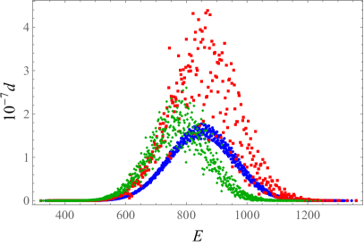
Figure 3: Plot of the degeneracy $d$ versus the energy $E$ for the spectra of the $A_{N-1}$ HS chain (3) with $J=2$ (red squares), the $D_{N}$ HS chain (8) with $J=1/2$ (green rhombuses) and the model (1) (blue circles) for $N=16$ spins and $m=3$ (left) or $m=4$ (right).

To make this observation more quantitative, we have computed the average degeneracy of the spectra of the latter models,

$$d_{\mathrm{av}}=\frac{m^{N}}{n}\,,$$

where $n$ denotes the number of distinct energy levels, for $m=3,4$ and $N=8,\dots,16$ spins. The results, which are presented in fig. 4, again clearly indicate that for sufficiently high $N$ the spectrum of the new model has a degeneracy similar to that of the $D_{N}$-type HS chain and is somewhat less degenerate than that of the original HS chain. It is also apparent from these plots that the degeneracy of the new chain grows exponentially with $N$, as is typically the case for Yangian-invariant models FG15 . All of these facts strongly suggest that the model (1) possesses some kind of (twisted) Yangian symmetry not only in the even $m$ case, as shown in the previous section, but also for odd $m$. This is typically the case for similar open chains with long-range interactions like the $BC_{N}$, $B_{N}$ and $D_{N}$ HS chains or the Simons–Altshuler model SA94 ; BPS95 ; TS15 and its integrable generalizations BFG16 .

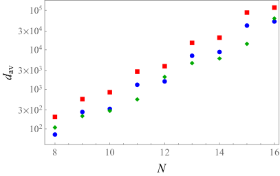
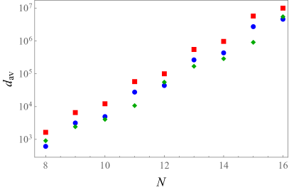
Figure 4: Logarithmic plot of the average degeneracy $d_{\mathrm{av}}$ of the spectra of the model (1) (blue dots), the HS chain (3) (red squares) and the $D_{N}$ HS chain (8) (green rhombuses) as a function of the number of spins $N$ for $8\leqslant N\leqslant 16$ and $m=3$ (left) or $m=4$ (right).

The plots in fig. 3 also seem to indicate that the level density of the new model (1) is Gaussian for sufficiently high $N$, as is the case for all spin chains of HS type EFGR05 ; EFG10 ; BFG09 ; BFG13 . This can be clearly seen for instance from fig. 5, where we have plotted both the histogram of the energy levels and the cumulative level density of the chain (1),

$$F(E)=\sum_{i;E_{i}\leqslant E}d(E_{i})\,,$$

where $d(E_{i})$ denotes the degeneracy of the $i$-th level $E_{i}$, for $N=16$ spins and $m=4$ (the case $m=3$ is completely similar). It is patent from fig. 5 that the latter density is virtually indistinguishable from the cumulative Gaussian distribution

$$G(E)=\frac{1}{2}\bigg{(}1+\operatorname{erf}\biggl{(}\frac{E-\mu}{\sqrt{2}\sigma}\biggr{)}\bigg{)}$$ (50)

with parameters $\mu$ and $\sigma$ respectively equal to the mean $\langle{\mathcal{H}}\rangle$ of the spectrum, given by eq. (49), and its standard deviation $(\langle{\mathcal{H}}^{2}\rangle-\langle{\mathcal{H}}\rangle^{2})^{1/2}$. As shown in appendix D, the latter quantity can also be evaluated in closed form, with the result

$$\langle{\mathcal{H}}^{2}\rangle-\langle{\mathcal{H}}\rangle^{2}=\frac{1}{180}\,\bigg{(}1-\frac{1}{m^{2}}\bigg{)}N(N^{2}-1)(2N^{2}+7)-\frac{1}{12m^{2}}\,N(N^{2}-1)(1-\pi(m))\,.$$ (51)

Note that (51) differs from its counterpart for the HS chain with $J=2$ computed in ref. FG05 , although both quantities do coincide at leading order $O(N^{5})$.

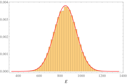
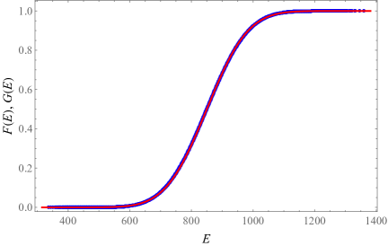
Figure 5: Left: histogram (normalized to unit area) of the degeneracies of the levels of the chain (1) with $m=4$ and $N=16$ spins compared to the Gaussian distribution (red line) with parameters $\mu$ and $\sigma$ respectively equal to the mean and the standard deviation of the model’s energy spectrum. Right: plot of the cumulative level density $F(E)$ of the latter model (blue dots) compared to the cumulative Gaussian distribution (50) (solid red line).

7 Conclusions and outlook

In this paper we have introduced a new class of open, translationally invariant spin chains with long-range interactions, which includes the original Haldane–Shastry chain as a particular (degenerate) case. The Hamiltonian of the new models, which contains both spin permutation and (polarized) spin reversal operators, turns out to be invariant under “twisted” translations combining an ordinary translation with a spin flip at one end of the chain. This remarkable invariance is one of the key properties shared by all members of the new class, regardless of the form of the spin-spin interactions. In fact, the models of this type are fundamentally different from all spin chains of Haldane–Shastry type studied so far, since their Hamiltonian cannot be obtained in the usual way from an extended root system. We have constructed a new elliptic chain of this class which smoothly interpolates between the twisted XXX Heisenberg model and what is perhaps the simplest model of the new type, in which the spin-spin exchange interaction is proportional to the inverse square of the (chord) distance. We have computed in closed form the partition function of the latter model applying Polychronakos’s freezing trick to a related spin dynamical model, whose spectrum we have also determined. When the number $m$ of internal degrees of freedom is even, the formula for the partition function implies that the new model is isomorphic to the sum of an $\mathrm{su}(1|1)$ and an $\mathrm{su}(m/2)$ (antiferromagnetic) HS chain Hamiltonian acting on the tensor product of their respective Hilbert spaces (cf. eq. (40)). In particular, this implies that the even $m$ model is symmetric under the direct sum of the Yangians $Y(\mathrm{gl}(1|1))$ and $Y(\mathrm{gl}(0|m/2))$. The latter property has also been used to derive a simple description of the spectrum in the even $m$ case in terms of a pair of independent Haldane motifs of types $\mathrm{su}(1|1)$ and $\mathrm{su}(0|m/2)$. With the help of the partition function, we have also analyzed the spectrum of the new chain for several values of $m$ and $N$, studying some of its main statistical properties. Our analysis clearly suggests that the level density is Gaussian for sufficiently large $N$, as is the case with spin chains of HS type. Moreover, our results indicate that the model’s spectrum has a huge degeneracy, comparable to that of well-known Yangian- or twisted Yangian-invariant models like the HS chain and its open versions. This is a strong indication that the new chain possesses an underlying (twisted) Yangian symmetry also in the odd $m$ case.

Our results open up several lines for future research. To begin with, the explicit description of the spectrum for even $m$ in terms of motifs makes it possible to study the thermodynamics of the model through the inhomogeneous transfer matrix approach successfully applied to similar chains EFG12 ; FGLR18 ; BBCFG19b . Finding an explicit realization of the generators of the Yangian symmetry group would also be highly desirable in this case. Another natural line of inquiry in this respect is to determine whether there is a similar motif-based description of the spectrum in the odd $m$ case. A related challenging and relevant open problem is to establish the existence of some kind of Yangian symmetry and its explicit form in the odd $m$ case which, as mentioned above, is suggested by the huge degeneracy of the spectrum, and thus prove the model’s integrability. It would also be of interest to find other solvable and/or integrable members of the new class introduced in this paper. For instance, the version with arbitrarily polarized spin reversal operators of the chain studied here, as well as its supersymmetric counterpart, should also be solvable with the method developed in this paper. Another problem worthy of investigation is the study of the (possibly partial) solvability of models with other spin-spin interactions, like the elliptic chain introduced in section 3.

As mentioned in the Introduction, the Hamiltonians of several spin chains with long-range interactions, including the original HS chain, are the parent Hamiltonians of infinite MPSs states (usually the ground state) constructed from certain rational CFTs like the $\mathrm{su}(m)_{1}$ WZNW model. Although the models introduced in this work share many properties with the latter spin chains, a crucial difference between both types of models is the presence of spin reversal operators in the Hamiltonian of the new ones. It would therefore be worth investigating whether the new models can also be constructed, at least in some cases, from appropriate CFTs, and if so what kind of CFTs would appear in this context. On a more speculative note, it could also be of interest to explore whether any of the new models are relevant in connection with the AdS-CFT conjecture, as has proved to be the case with other translationally invariant spin chains like the Inozemtsev chain.

Appendix A Auxiliary Hamiltonian $H^{\prime}$ and Dunkl operators

In this appendix we introduce an auxiliary scalar operator $H^{\prime}$ that shall be used in appendix B to compute the spectrum of the dynamical Hamiltonian $H$ in eq. (9). A key property of this operator is the fact that it can be expressed as the sum of the squares of a certain family of commuting Dunkl operators, explicitly defined in the second part of this appendix.

More precisely, let us define

$$H^{\prime}=-\Delta+2a\sum_{i<j}\bigg{[}\frac{a-K_{ij}}{\sin^{2}(x_{i}-x_{j})}+\frac{a-\widetilde{K}_{ij}}{\cos^{2}(x_{i}-x_{j})}\bigg{]}\,,$$ (52)

where $K_{ij}$ denotes the coordinate permutation operator acting on a scalar function $f(\mathbf{x})$ as

$$(K_{ij}f)(x_{1},\dots,x_{i},\dots,x_{j},\dots,x_{N})=f(x_{1},\dots,x_{j},\dots,x_{i},\dots x_{N})\,,$$ (53)

$\widetilde{K}_{ij}:=K_{ij}K_{i}K_{j}$, and $K_{l}$ is the translation operator defined by

$$(K_{l}f)(x_{1},\dots,x_{l},\dots,x_{N})=f(x_{1},\dots,x_{l}+\pi/2,\dots,x_{N})\,.$$ (54)

Note that the operator $K_{l}$ is obviously related to the star operator defined in section 2 by $z_{l}^{*}=\mathrm{e}^{2\mathrm{i}(K_{l}x_{l})}$. Before proceeding further, a comment on the domain of the operator $H^{\prime}$ is in order. Indeed, the presence of the operators $K_{ij}$ and $K_{i}K_{j}$ in $H^{\prime}$ entails that we have to enlarge its natural configuration space (10) to a region invariant under the action of the latter operators. To begin with, the invariance under the permutation operators $K_{ij}$ leads to the region

$$A^{\prime}=\{\mathbf{x}\in{\mathbb{R}}^{N}:|x_{i}-x_{j}|<\pi/2,\enspace 1\leqslant i<j\leqslant N\}.$$

On the other hand, for the operators $K_{ij}$ and $K_{i}K_{j}$ to generate the Weyl group of $D_{N}$ type, it is necessary that $(K_{i}K_{j})^{2}=1$ for all $i\neq j$. In fact, as will become clear in the sequel, the stronger condition $K_{i}^{2}=1$ for all $i$ is actually needed in what follows. In view of this condition it is intuitively clear that we must take as configuration space of $H^{\prime}$ the region $A^{\prime}$, identifying $\mathbf{x}$ with $\mathbf{x}+\pi\mathbf{e}_{i}$ in the definition of $K_{i}$. In a more technical language, we shall take as domain of $H^{\prime}$ an appropriate dense subspace ${\mathcal{P}}$ of the Hilbert space

$${\mathfrak{H}}^{\prime}=L^{2}([-\pi/2,\pi/2]^{N}\cap A^{\prime})$$

on which $K_{i}^{2}=1$ for all $i$ (see figure 6 for a sketch of the configuration space $[-\pi/2,\pi/2]^{N}\cap A^{\prime}$ in two and three dimensions). The space ${\mathcal{P}}$ will be chosen as the span of the $\pi$-periodic trigonometric functions

$$\varphi_{\mathbf{n}}(\mathbf{x})=\mu(\mathbf{x})\mathrm{e}^{2\mathrm{i}\mathbf{n}\cdot\mathbf{x}}\,,\qquad\mathbf{n}:=(n_{1},\dots,n_{N})\in{\mathbb{Z}}^{N}\,,$$ (55)

where the factor

$$\mu=\prod_{í<j}\big{|}\sin\bigl{(}2(x_{i}-x_{j})\bigr{)}\big{|}^{a}$$ (56)

(which, as we shall see, is the ground state of $H^{\prime}$) is included for later convenience. Indeed, the span of the functions (55) is dense in $L^{2}([-\pi/2,\pi/2]^{N})$, and hence in ${\mathfrak{H}}^{\prime}$. It is also important to realize that the conditions $K_{i}^{2}=1$ for all $i$ on ${\mathcal{P}}$ entail the quantization of the system’s total momentum, which causes the spectrum of $H^{\prime}$ on ${\mathfrak{H}}^{\prime}$ to be discrete.

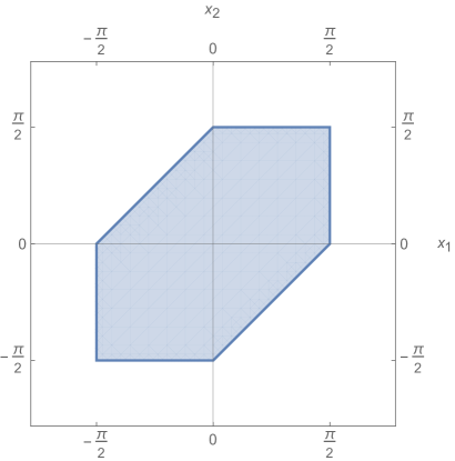
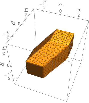
Figure 6: Configuration space $A^{\prime}\cap[-\pi/2,\pi/2]^{N}$ of the auxiliary operator $H^{\prime}$ for $N=2$ (left) and $N=3$ (right). In general, the configuration space is an irregular $N$-polytope with $N(N+1)$ faces.

We next introduce the differential-difference Dunkl operators Du98 ; FGGRZ01b

$$J_{l}=\mathrm{i}\,\frac{\partial}{\partial x_{l}}-a\bigg{\{}\mathrm{i}\sum_{\mathchoice{\hbox to0.0pt{\hss$\displaystyle{j;j\neq l}$\hss}}{\hbox to0.0pt{\hss$\textstyle{j;j\neq l}$\hss}}{\hbox to0.0pt{\hss$\scriptstyle{j;j\neq l}$\hss}}{\hbox to0.0pt{\hss$\scriptscriptstyle{j;j\neq l}$\hss}}}\big{[}\cot(x_{l}-x_{j})K_{lj}-\tan(x_{l}-x_{j})\widetilde{K}_{lj}\big{]}+\sum_{j=1}^{l-1}(K_{lj}+\widetilde{K}_{lj})-\sum_{\mathchoice{\hbox to0.0pt{\hss$\displaystyle{j=l+1}$\hss}}{\hbox to0.0pt{\hss$\textstyle{j=l+1}$\hss}}{\hbox to0.0pt{\hss$\scriptstyle{j=l+1}$\hss}}{\hbox to0.0pt{\hss$\scriptscriptstyle{j=l+1}$\hss}}}^{N}(K_{lj}+\widetilde{K}_{lj})\bigg{\}},$$ (57)

where $l=1,\dots,N$ and $K_{lj}=K_{jl}$ for $l>j$. The operators $J_{l}$ are related to the analogous operators $J_{l}^{0}(\mathbf{z})$ in ref. FGGRZ01b by

$$J_{l}=-2\mu\,J_{l}^{0}(\mathbf{z})\mu^{-1}-a\sum_{j=1}^{l-1}(K_{lj}+\widetilde{K}_{lj})+a\sum_{\mathchoice{\hbox to0.0pt{\hss$\displaystyle{j=l+1}$\hss}}{\hbox to0.0pt{\hss$\textstyle{j=l+1}$\hss}}{\hbox to0.0pt{\hss$\scriptstyle{j=l+1}$\hss}}{\hbox to0.0pt{\hss$\scriptscriptstyle{j=l+1}$\hss}}}^{N}(K_{lj}+\widetilde{K}_{lj}),$$ (58)

where $\mathbf{z}:=(z_{1},\dots,z_{N})$ with $z_{k}=\mathrm{e}^{2\,\mathrm{i}x_{k}}$ and the inessential parameter $m$ in the latter reference has been set to $0$. Note also that the action of the operator $K_{i}$ on the variable $z_{i}$ is simply $K_{i}z_{i}=z_{i}^{*}=-z_{i}$, akin to the action of $S_{i}$ on the spin variable $s_{i}$. This observation, in fact, lends additional motivation to the definition of the action of $K_{i}$ on the physical coordinate $x_{i}$ as a translation by $\pi/2$.

A long but standard explicit computation shows that the operators $J_{i}$ —unlike their counterparts $J_{l}^{0}(\mathbf{z})$— form a commuting family, i.e.,

$$[J_{i},J_{j}]=0\,,\qquad\forall i,j=1,\dots,N\,.$$

It should be noted that for $N\geqslant 3$ it is essential for the validity of this result that the operators $K_{i}$ satisfy $K_{i}^{2}=1$, as opposed to the weaker condition $(K_{i}K_{j})^{2}=1$ for all $i\neq j$ stemming from the $D_{N}$ Weyl group algebra. Moreover, a similar calculation proves that the auxiliary operator $H^{\prime}$ can be expressed in terms of the Dunkl operators $J_{i}$ as

$$H^{\prime}=\sum_{i}J_{i}^{2}\,.$$ (59)

Again, for $N\geqslant 3$ the above identity requires that $K_{i}^{2}=1$ for all $i$. In appendix B we shall rely on eq. (59) to explicitly compute the spectrum of $H^{\prime}$ on ${\mathfrak{H}}^{\prime}$. This result will then be used in section 4 to derive the spectrum of the spin dynamical model $H$ in the CM frame.

Appendix B Spectrum of the dynamical models $H^{\prime}$ and $H|_{{\mathfrak{H}}}$

In this appendix we shall first compute the spectrum of the auxiliary Hamiltonian $H^{\prime}$ in its natural Hilbert space ${\mathfrak{H}}^{\prime}$. We shall then use this result to derive the spectrum of the Hamiltonian $H$ in a suitable subspace of ${\mathfrak{H}}\subset{\mathfrak{H}}^{\prime}\otimes\Sigma$, in which the action of the latter operator coincides with that of $H^{\prime}$.

B.1 Spectrum of $H^{\prime}$

The starting point in the computation of the spectrum of $H^{\prime}$ on ${\mathfrak{H}}^{\prime}$ is the fact that the operators $J_{l}$ leave invariant the (infinite-dimensional) subspace ${\mathcal{P}}_{n}\subset{\mathcal{P}}$ spanned by the functions $\varphi_{\mathbf{n}}(\mathbf{x})$ with $|\mathbf{n}|:=\sum_{i}n_{i}=n$, for an arbitrary (possibly negative) integer $n$. In fact, the operators $J_{l}$ also admit the finite-dimensional invariant subspaces ${\mathcal{R}}_{p}$ ($p=0,1,\dots$) spanned by the latter monomials with multiindices satisfying the conditions $|n_{i}|\leqslant p$ for $i=1,\dots,N$. By eq. (59), the auxiliary operator $H^{\prime}$ will also leave invariant the subspaces ${\mathcal{P}}_{n}$ and ${\mathcal{R}}_{p}$, and hence their intersection. We shall construct a non-orthonormal (i.e., Schauder) basis ${\mathcal{B}}$ of ${\mathfrak{H}}^{\prime}$ by appropriately ordering the set $\{\varphi_{\mathbf{n}}(\mathbf{x}):\mathbf{n}\in{\mathbb{Z}}^{N}\}$, and then show that the operator $H^{\prime}$ is upper triangular with respect to this basis. Finally, we shall derive the spectrum of $H^{\prime}$ by explicitly computing its diagonal matrix elements in the basis ${\mathcal{B}}$.

In order to simplify the calculation, we shall apply the change of variables $z_{k}=\mathrm{e}^{2\,\mathrm{i}x_{k}}$ and the pseudo-gauge transformation with gauge factor $\mu$ to the Dunkl operators $J_{l}$, and thus work with the operators

$$J_{i}^{*}:=\mu^{-1}J_{i}\,\mu=-2z_{i}\frac{\partial}{\partial z_{i}}-a\sum_{j;j\neq i}\bigg{[}\frac{z_{i}+z_{j}}{z_{i}-z_{j}}\,(1-K_{ij})+\frac{z_{i}-z_{j}}{z_{i}+z_{j}}\,(1-\widetilde{K}_{ij})+\operatorname{sgn}(i-j)(K_{ij}+\widetilde{K}_{ij})\bigg{]},$$

where $\operatorname{sgn}(x)$ is the sign of $x$. Defining

$$\phi_{\mathbf{n}}(\mathbf{z})=\mu(\mathbf{x})^{-1}\varphi_{\mathbf{n}}(\mathbf{x})=\prod_{k}z_{k}^{n_{k}},$$ (60)

where $n_{k}\in{\mathbb{Z}}$, we then have

$$J_{i}\varphi_{\mathbf{n}}=\mu J_{i}^{*}\phi_{\mathbf{n}}\,.$$

It shall also be necessary for what follows to define a partial order in the set of monomials $\phi_{\mathbf{n}}$. This is done in four stages, as we shall now explain. To begin with, we order the multiindices $\mathbf{n}\in{\mathbb{Z}}^{N}$ by $p(\mathbf{n}):=\max\{|n_{i}|:i=1,\dots,N\}$, and then (for $p(\mathbf{n})=p(\mathbf{n}^{\prime})$) by $n:=\sum_{i}n_{i}$. We next define $[\mathbf{n}]\in{\mathbb{Z}}^{N}$ as the rearrangement of the multiindex $\mathbf{n}\in{\mathbb{Z}}^{N}$ whose components are weakly decreasing, i.e., such that $[\mathbf{n}]_{1}\geqslant[\mathbf{n}]_{2}\geqslant\cdots\geqslant[\mathbf{n}]_{N}$. The multiindices with given $p(\mathbf{n})$ and $n$ are then partially ordered using their rearrangements $[\mathbf{n}]$, i.e., defining that $\mathbf{n}$ precedes $\mathbf{n}^{\prime}$ if the first nonzero difference $[\mathbf{n}]_{i}-[\mathbf{n}^{\prime}]_{i}$ is negative. The above prescription clearly defines a total order among weakly decreasing multiindices and a partial order in ${\mathbb{Z}}^{N}$ which we shall denote by $\prec\,$, with $0\equiv(0,\dots,0)$ as first element. We shall then say that $\phi_{\mathbf{n}}\prec\phi_{\mathbf{n}^{\prime}}$ if and only if $\mathbf{n}\prec\mathbf{n}^{\prime}$. We shall also use the notation $\mathbf{n}\preceq\mathbf{n}^{\prime}$ to indicate that $\mathbf{n}^{\prime}\not\prec\mathbf{n}$ (i.e., either $\mathbf{n}\prec\mathbf{n}^{\prime}$ or $[\mathbf{n}]=[\mathbf{n}^{\prime}]$), and similarly for $\phi_{\mathbf{n}}\preceq\phi_{\mathbf{n}^{\prime}}$. It is obvious from the previous definition that the partial order thus defined is invariant under coordinate permutations, i.e.,

$$\phi_{\mathbf{n}}\prec\phi_{\mathbf{n}^{\prime}}\enspace\implies\enspace W\phi_{\mathbf{n}}\prec W\phi_{\mathbf{n}^{\prime}}$$

where $W$ is an arbitrary element of the permutation group generated by the operators $K_{ij}$. Of course, the partial order $\prec$ can be equivalently defined on the functions $\varphi_{\mathbf{n}}$ by setting $\varphi_{\mathbf{n}}\prec\varphi_{\mathbf{n}^{\prime}}$ if and only if $\mathbf{n}\prec\mathbf{n}^{\prime}$. Note, finally, that $\prec$ can be promoted to a total order by setting the precedence of two multiindices which differ by a permutation of their components in an arbitrary way. For instance, if we choose lexicographic order then $(-1,\dots,-1)$ is the second element (this is always the case due to the partial order), $(-1,\dots,-1,0)$ is the third, $(-1,\dots,-1,0,-1)$ the fourth, etc.

We start by computing $J_{i}^{*}\phi_{\mathbf{n}}$ on a monomial $\phi_{\mathbf{n}}$. To this end, note first of all that

$$\frac{z_{i}+z_{j}}{z_{i}-z_{j}}\,(1-K_{ij})z_{i}^{n_{i}}z_{j}^{n_{j}} =(z_{i}+z_{j})\,\frac{z_{i}^{n_{i}}z_{j}^{n_{j}}-z_{i}^{n_{j}}z_{j}^{n_{i}}}{z_{i}-z_{j}}$$

$$=\operatorname{sgn}(n_{i}-n_{j})(z_{i}z_{j})^{\min(n_{i},n_{j})}(z_{i}+z_{j})\,\frac{z_{i}^{|n_{i}-n_{j}|}-z_{j}^{|n_{i}-n_{j}|}}{z_{i}-z_{j}},$$

where by definition $\operatorname{sgn}(0)=0$. Since the exponents in the numerator are nonnegative we can carry out the division, thus easily obtaining

$$\frac{z_{i}+z_{j}}{z_{i}-z_{j}}\,(1-K_{ij})z_{i}^{n_{i}}z_{j}^{n_{j}}=\operatorname{sgn}(n_{i}-n_{j})\Big{(}z_{i}^{n_{i}}z_{j}^{n_{j}}+z_{i}^{n_{j}}z_{j}^{n_{i}}\\ +2\sum_{k=1}^{|n_{i}-n_{j}|-1}z_{i}^{\max(n_{i},n_{j})-k}z_{j}^{\min(n_{i},n_{j})+k}\Big{)}.$$ (61)

Similarly,

$$\frac{z_{i}-z_{j}}{z_{i}+z_{j}}\,(1-\widetilde{K}_{ij})z_{i}^{n_{i}}z_{j}^{n_{j}}=(-1)^{n_{j}}\operatorname{sgn}(n_{i}-n_{j})\Big{(}z_{i}^{n_{i}}(-z_{j})^{n_{j}}+z_{i}^{n_{j}}(-z_{j})^{n_{i}}\\ +2\sum_{k=1}^{|n_{i}-n_{j}|-1}z_{i}^{\max(n_{i},n_{j})-k}(-z_{j})^{\min(n_{i},n_{j})+k}\Big{)},$$ (62)

and

$$(K_{ij}+\widetilde{K}_{ij})z_{i}^{n_{i}}z_{j}^{n_{j}}=z_{i}^{n_{j}}z_{j}^{n_{i}}\big{(}1+(-1)^{n_{i}+n_{j}}\big{)}.$$ (63)

Note, in particular, that the right-hand side of eqs. (61)–(63) obviously belongs to ${\mathcal{P}}_{n}^{*}:=\mu^{-1}{\mathcal{P}}_{n}$ with $n=|\mathbf{n}|$, i.e., the space spanned by monomials $\phi_{\mathbf{n}}$ with integer exponents $n_{k}$ ($k=1,\dots,N$) of total degree $|\mathbf{n}|=n$. Hence $J_{i}^{*}{\mathcal{P}}_{n}^{*}\subset{\mathcal{P}}_{n}^{*}$, or equivalently $J_{i}{\mathcal{P}}_{n}\subset{\mathcal{P}}_{n}$, as we had previously claimed. In the same way it is established that $J_{i}^{*}{\mathcal{R}}_{p}^{*}\subset{\mathcal{R}}_{p}^{*}:=\mu^{-1}{\mathcal{R}}_{p}$, and hence $J_{i}{\mathcal{R}}_{p}\subset{\mathcal{R}}_{p}$. It is also easy to convince oneself that all the terms in the sums in eqs. (61)-(62) precede the monomial $z_{i}^{n_{i}}z_{j}^{n_{j}}$ with respect to the partial order defined above, since the exponents of $z_{i}$ and $z_{j}$ in each of them range over $\min(n_{i},n_{j})+1$ and $\max(n_{i},n_{j})-1$ and their sum equals $n_{i}+n_{j}$. This is easily seen to imply that

$$\frac{z_{i}+z_{j}}{z_{i}-z_{j}}\,(1-K_{ij})\phi_{\mathbf{n}} =\operatorname{sgn}(n_{i}-n_{j})(z_{i}^{n_{i}}z_{j}^{n_{j}}+z_{i}^{n_{j}}z_{j}^{n_{i}})\prod_{k;k\neq i,j}z_{k}^{n_{k}}+\text{l.o.t.}\,,$$ (64)

$$\frac{z_{i}-z_{j}}{z_{i}+z_{j}}\,(1-\widetilde{K}_{ij})\phi_{\mathbf{n}} =\operatorname{sgn}(n_{i}-n_{j})\big{(}z_{i}^{n_{i}}z_{j}^{n_{j}}+(-1)^{n_{i}+n_{j}}z_{i}^{n_{j}}z_{j}^{n_{i}}\big{)}\prod_{k;k\neq i,j}z_{k}^{n_{k}}+\text{l.o.t.}\,,$$ (65)

where l.o.t. stands for a linear combination of monomials preceding $\phi_{\mathbf{n}}$. From eqs. (63)–(65) it immediately follows that $\phi_{\mathbf{n}}$ does not precede any monomial in $J_{i}^{*}\phi_{\mathbf{n}}$, i.e., $J_{i}^{*}\phi_{\mathbf{n}}$ is of the form

$$J_{i}^{*}\phi_{\mathbf{n}}=\sum_{\mathbf{n}^{\prime}\preceq\mathbf{n}}c_{\mathbf{n}^{\prime}\mathbf{n}}\phi_{\mathbf{n}^{\prime}}$$ (66)

for appropriate coefficients $c_{\mathbf{n}^{\prime}\mathbf{n}}\in{\mathbb{C}}^{N}$.

The last observation can be considerably strengthened if we assume that $\mathbf{n}\in\big{[}{\mathbb{Z}}^{N}\big{]}$, i.e., if $n_{1}\geqslant n_{2}\geqslant\cdots\geqslant n_{N}$. Indeed, in this case

$$\operatorname{sgn}(n_{i}-n_{j})=(1-\delta_{n_{i}n_{j}})\operatorname{sgn}(j-i),$$

so that the coefficient of $z_{i}^{n_{j}}z_{j}^{n_{i}}$ in

$$\bigg{(}\frac{z_{i}+z_{j}}{z_{i}-z_{j}}\,(1-K_{ij})+\frac{z_{i}-z_{j}}{z_{i}+z_{j}}\,(1-\widetilde{K}_{ij})+\operatorname{sgn}(i-j)(K_{ij}+\widetilde{K}_{ij})\bigg{)}z_{i}^{n_{i}}z_{j}^{n_{j}}$$

equals

$$\big{[}\operatorname{sgn}(j-i)(1-\delta_{n_{i}n_{j}})+\operatorname{sgn}(i-j)\big{]}\big{(}1+(-1)^{n_{i}+n_{j}}\big{)}=2\delta_{n_{i}n_{j}}\operatorname{sgn}(i-j)$$

and therefore

$$\bigg{(}\frac{z_{i}+z_{j}}{z_{i}-z_{j}}\,(1-K_{ij})+\frac{z_{i}-z_{j}}{z_{i}+z_{j}}\,(1-\widetilde{K}_{ij})+\operatorname{sgn}(i-j)(K_{ij}+\widetilde{K}_{ij})\bigg{)}z_{i}^{n_{i}}z_{j}^{n_{j}}\\ =2\operatorname{sgn}(j-i)(1-2\delta_{n_{i}n_{j}})z_{i}^{n_{i}}z_{j}^{n_{j}}+\text{l.o.t.}$$

Multiplying both sides of the latter equation by $\prod_{k;k\neq i,j}z_{k}^{n_{k}}$ we finally obtain

$$J_{i}^{*}\phi_{\mathbf{n}}=\lambda_{i}(\mathbf{n})\phi_{\mathbf{n}}+\text{l.o.t.},$$ (67)

where l.o.t. consists of monomials $\phi_{\mathbf{n}^{\prime}}\prec\phi_{\mathbf{n}}$ and

$$\lambda_{i}(\mathbf{n}) =-2n_{i}+2a\sum_{j;j\neq i}\operatorname{sgn}(i-j)(1-2\delta_{n_{i},n_{j}})$$

$$=-2n_{i}+2a(2i-N-1)+4a\big{|}\{j:j>i,\ n_{i}=n_{j}\}\big{|}-4a\big{|}\{j:j<i,\ n_{i}=n_{j}\}\big{|},$$

with $|A|$ denoting the cardinal of a set $A$. The above formula can be slightly simplified by introducing the notation

$$l(n_{i})=\min\{j:n_{j}=n_{i}\}\,,\qquad\#(n_{i})=|\{j:n_{j}=n_{i}\}|,$$

in terms of which

$$\lambda_{i}(\mathbf{n})=-2n_{i}+2a\big{[}4l(n_{i})+2\#(n_{i})-2i-N-3\big{]}\,.$$ (68)

We shall next make use of eqs. (66)-(68) above to obtain the spectrum of $H^{\prime}$. More precisely, we shall see that the action of $H^{\prime}$ is upper triangular on the (non-orthonormal) basis ${\mathcal{B}}=\{\varphi_{\mathbf{n}}:\mathbf{n}\in{\mathbb{Z}}\}$ of ${\mathfrak{H}}^{\prime}$, ordered with any ordering compatible with $\prec$, and shall explicitly compute its diagonal matrix elements.

We start by evaluating $H^{\prime}\varphi_{\mathbf{n}}$ when the multiindex $\mathbf{n}$ belongs to $[{\mathbb{Z}}^{N}]$, i.e., is non-increasing. To this end, note first of all that

$$H^{\prime}\varphi_{\mathbf{n}}=\mu\cdot(\mu^{-1}H^{\prime}\mu)\phi_{\mathbf{n}}=\mu\sum_{i}(J_{i}^{*})^{2}\phi_{\mathbf{n}}\,.$$

Since by assumption $\mathbf{n}\in[{\mathbb{Z}}^{N}]$, by eq. (67) we have

$$(J_{i}^{*})^{2}\phi_{\mathbf{n}}=\lambda_{i}(\mathbf{n})J_{i}^{*}\phi_{n}+J_{i}^{*}(\text{l.o.t})=\lambda_{i}(\mathbf{n})J_{i}^{*}\phi_{\mathbf{n}}+\text{l.o.t.}=\lambda_{i}(\mathbf{n})^{2}\phi_{\mathbf{n}}+\text{l.o.t.}\,,$$

where in the second equality we have used eq. (66). Hence in this case

$$H^{\prime}\varphi_{\mathbf{n}}=\Big{(}\sum_{i}\lambda_{i}(\mathbf{n})^{2}\Big{)}\varphi_{\mathbf{n}}+\text{l.o.t.}$$ (69)

The coefficient of $\varphi_{\mathbf{n}}$ in the latter formula can be simplified by noting that

$$\sum_{j=l(n_{i})}^{l(n_{i})+\#(n_{i})-1}\lambda_{j}(\mathbf{n})^{2}=4\sum_{k=l(n_{i})}^{l(n_{i})+\#(n_{i})-1}\Big{[}n_{k}+a(N-2k+1)\Big{]}^{2},$$

where we have performed the change of index $k=2l(n_{i})+\#(n_{i})-j-1$ and used the fact that $n_{k}=n_{i}$ for $l(n_{i})\leqslant k\leqslant l(n_{i})+\#(n_{i})-1$. We thus obtain

$$\sum_{i}\lambda_{i}(\mathbf{n})^{2}=4\sum_{i}\Big{[}n_{i}+a(N-2i+1)\Big{]}^{2}=:E(\mathbf{n})\,.$$ (70)

We shall finally compute $H^{\prime}$ on a basis function $\varphi_{\mathbf{n}}$ with an arbitrary $\mathbf{n}\in{\mathbb{Z}}^{N}$. To this end, let us denote by $W$ any permutation such that $\varphi_{\mathbf{n}}=W\varphi_{[\mathbf{n}]}$. Since the auxiliary operator $H^{\prime}$ clearly commutes with $K_{ij}$ for all $i\neq j$, it also commutes with any permutation $W$. We thus have

$$H^{\prime}\varphi_{\mathbf{n}}=WH^{\prime}\varphi_{[\mathbf{n}]}=E([\mathbf{n}])W\varphi_{[\mathbf{n}]}+W(\text{l.o.t.})=E([\mathbf{n}])\varphi_{\mathbf{n}}+\text{l.o.t.},$$

where we have used the fact that the partial order $\prec$ is invariant under permutations. We conclude that $H^{\prime}$ is indeed represented by an upper triangular matrix in the basis ${\mathcal{B}}$ of ${\mathfrak{H}}^{\prime}$, with eigenvalues $E([\mathbf{n}])$ with $\mathbf{n}\in{\mathbb{Z}}^{N}$. Moreover, since $H^{\prime}$ preserves the subspace ${\mathcal{P}}_{n}$ for all integers $n$, ${\mathfrak{H}}^{\prime}$ admits a basis of (unnormalized) eigenfunctions of $H^{\prime}$ of the form

$$\psi_{\mathbf{n}}=\varphi_{\mathbf{n}}+\sum_{\mathbf{n}^{\prime}\prec\mathbf{n},\,|\mathbf{n}^{\prime}|=|\mathbf{n}|}c_{\mathbf{n}^{\prime}\mathbf{n}}\varphi_{\mathbf{n}^{\prime}}\,,\qquad\mathbf{n}\in{\mathbb{Z}}^{N}\,.$$ (71)

Note that the sum over $\mathbf{n}^{\prime}$ in the previous equation is actually finite, since $\max_{i}|n^{\prime}_{i}|\leqslant p(\mathbf{n})$ by the invariance of the subspaces ${\mathcal{R}}_{p}$ under $H^{\prime}$. On the other hand, the auxiliary operator $H^{\prime}$ (as well as its counterparts $H$ and $H_{\mathrm{sc}}$ in the previous section) is translationally invariant, and thus commutes with the total momentum operator

$$P=-\mathrm{i}\sum_{j}\frac{\partial}{\partial x_{j}}\,.$$

Since obviously $P\varphi_{\mathbf{n}^{\prime}}=2|\mathbf{n}^{\prime}|\varphi_{\mathbf{n}^{\prime}}=2|\mathbf{n}|\varphi_{\mathbf{n}^{\prime}}$, the states (71) are also eigenfunctions of $P$ with eigenvalue $2|\mathbf{n}|$. It follows that the set $\{\psi_{\mathbf{n}}:\mathbf{n}\in{\mathbb{Z}}^{N}\}$ is a (non-orthonormal) basis of ${\mathfrak{H}}^{\prime}$ consisting of common eigenfunctions of $H^{\prime}$ and $P$, with

$$H^{\prime}\psi_{\mathbf{n}}=E([\mathbf{n}])\psi_{\mathbf{n}}\,,\qquad P\psi_{\mathbf{n}}=2|\mathbf{n}|\psi_{\mathbf{n}}\,.$$ (72)

Note, finally that if $\psi$ is an eigenfunction of $P$ and $H^{\prime}$ with respective eigenvalues $p$ and $E$, it is straightforward to check that $\mathrm{e}^{2\mathrm{i}\mskip 1.0muc|\mathbf{x}|}\psi$ (where $|\mathbf{x}|:=\sum_{k}x_{k}$) is an eigenfunction of the latter operators with eigenvalues $p+2Nc$ and $E+4cp+4Nc^{2}$. From this fact and eq. (71) it follows that

$$\psi_{\mathbf{n}+c\mathbf{1}}(\mathbf{x})=\mathrm{e}^{2\mathrm{i}\mskip 1.0muc|\mathbf{x}|}\psi_{\mathbf{n}}(\mathbf{x})\,,\qquad\mathbf{1}:=(1,\dots,1)\,.$$ (73)

B.2 Spectrum of $H$ on ${\mathfrak{H}}$

As before, we start by extending the natural Hilbert space $L^{2}(A)\otimes\Sigma$ of the Hamiltonian $H$ of the spin dynamical model (9) to ${\mathfrak{H}}^{\prime}\otimes\Sigma$. It is then clear from its definition that $H$ coincides with the auxiliary operator $H^{\prime}$ in the subspace ${\mathfrak{H}}$ of ${\mathfrak{H}}^{\prime}\otimes\Sigma$ defined by the relations

$$K_{ij}=-S_{ij},\qquad K_{i}K_{j}=S_{i}S_{j},$$

i.e., whose elements are i) antisymmetric under simultaneous permutations of the coordinates and spin variables, and ii) symmetric under translations by $\pi/2$ (modulo $\pi$) of an even number of particles’ coordinates and reversal of their corresponding spins. This subspace is therefore

$${\mathfrak{H}}=\Lambda_{a}\Lambda_{0}({\mathfrak{H}}^{\prime}\otimes\Sigma)\,,$$

where $\Lambda_{a}$ and $\Lambda_{0}$ respectively denote the antisymmetrizer with respect to coordinate and spin permutations and the symmetrizer with respect to the operators $K_{i}S_{i}K_{j}S_{j}$. It is important to note that the spectrum of $H$ on ${\mathfrak{H}}$ is actually the same as its spectrum on the more natural Hilbert space $L^{2}([-\pi/2,\pi/2]\cap A)\otimes\Sigma$. Indeed, what we are basically doing here is enlarging the original configuration space $A$ to $A^{\prime}$ by applying the Weyl group generated by the operators $K_{ij}$, $K_{i}K_{j}$, and then restricting ourselves to wavefunctions defined on this larger space with a certain well-defined symmetry under the action of the corresponding operators $K_{ij}S_{ij}$, $K_{i}S_{i}K_{j}S_{j}$ (see, e.g., ref. BFG11 for a more technical explanation).

The symmetrizer $\Lambda_{0}$ can be expressed in terms of the projectors $\Lambda_{0}^{\pm}$ onto states symmetric (“$+$”) or antisymmetric (“$-$”) under the action of the operators $K_{i}S_{i}$, defined by

$$\Lambda_{0}^{\pm}=\frac{1}{2^{N}}\left(\sum_{i=1}^{2^{N-1}}W_{i}^{+}\pm\sum_{i=1}^{2^{N-1}}W_{i}^{-}\right),$$

where $W_{i}^{+}$ (respectively $W_{i}^{-}$) denotes the product of an even (respectively odd) number of operators $K_{i}S_{i}$, as

$$\Lambda_{0}=\frac{1}{2^{N-1}}\sum_{i=1}^{2^{N-1}}W_{i}^{+}=\Lambda_{0}^{+}+\Lambda_{0}^{-}\,.$$

We thus have

$${\mathfrak{H}}=\Lambda_{a}\Lambda_{0}^{+}({\mathfrak{H}}^{\prime}\otimes\Sigma)\oplus\Lambda_{a}\Lambda_{0}^{-}({\mathfrak{H}}^{\prime}\otimes\Sigma)\,.$$

A basis of ${\mathfrak{H}}$ consists therefore of the states

$$\Phi^{\varepsilon}_{\mathbf{n},\mathbf{s}}=\Lambda_{a}\Lambda_{0}^{\varepsilon}(\varphi_{\mathbf{n}}(\mathbf{x})|\mathbf{s}\rangle)\,,$$ (74)

where $\mathbf{n}\in{\mathbb{Z}}^{N}$ and $\mathbf{s}\in\{-M,-M+1,\dots,M\}^{N}$ must be appropriately restricted so that the latter states are linearly independent. For instance, it suffices that

1. $n_{1}\geqslant\cdots\geqslant n_{N}$

2. $\displaystyle n_{i}=n_{j}\implies s_{i}>s_{j}$

3. $s_{i}\geqslant 0$ for all $i$, and $s_{i}>0$ if $(-1)^{n_{i}}\varepsilon=-1$ .

Indeed, the first two conditions simply take into account the antisymmetry of $\Phi_{\mathbf{n},\mathbf{s}}^{\varepsilon}$ with respect to simultaneous permutations of spatial coordinates and spins. As to the third one, note first of all that acting on $\Phi^{\varepsilon}_{\mathbf{n},\mathbf{s}}$ with $K_{i}S_{i}$ (which does not change the physical state, since by construction $K_{i}S_{i}\Phi^{\varepsilon}_{\mathbf{n},\mathbf{s}}=\varepsilon\Phi^{\varepsilon}_{\mathbf{n},\mathbf{s}}$) we can reverse the sign of $s_{i}$ if necessary. Moreover, if $s_{i}=0$ we have

$$K_{i}S_{i}\Phi^{\varepsilon}_{\mathbf{n},\mathbf{s}}=(-1)^{n_{i}}\Phi^{\varepsilon}_{\mathbf{n},\mathbf{s}}=\varepsilon\Phi^{\varepsilon}_{\mathbf{n},\mathbf{s}}\,,$$

so that $(-1)^{n_{i}}\varepsilon=1$. By the same token, the states

$$\Psi^{\varepsilon}_{\mathbf{n},\mathbf{s}}=\Lambda_{a}\Lambda_{0}^{\varepsilon}(\psi_{\mathbf{n}}(\mathbf{x})|\mathbf{s}\rangle)\,,$$

where the quantum numbers $\mathbf{n}$ and $\mathbf{s}$ satisfy conditions 1–3 above, are also a basis of ${\mathfrak{H}}$. Since, again by construction,

$$H^{\prime}\Lambda_{a}\Lambda_{0}^{\varepsilon}=H\Lambda_{a}\Lambda_{0}^{\varepsilon}\,,$$

and

$$[H^{\prime},K_{ij}]=[H^{\prime},K_{i}]=0\enspace\implies\enspace[H^{\prime},\Lambda_{a}]=[H^{\prime},\Lambda_{0}^{\varepsilon}]=0\,,$$

we have

$$H\Psi^{\varepsilon}_{\mathbf{n},\mathbf{s}} =H\Lambda_{a}\Lambda_{0}^{\varepsilon}(\psi_{\mathbf{n}}|\mathbf{s}\rangle)=H^{\prime}\Lambda_{a}\Lambda_{0}^{\varepsilon}(\psi_{\mathbf{n}}|\mathbf{s}\rangle)=\Lambda_{a}\Lambda_{0}^{\varepsilon}\big{(}(H^{\prime}\psi_{\mathbf{n}})|\mathbf{s}\rangle\big{)}$$

$$=\Lambda_{a}\Lambda_{0}^{\varepsilon}\big{(}E(\mathbf{n})\psi_{\mathbf{n}}|\mathbf{s}\rangle\big{)}=E(\mathbf{n})\Psi^{\varepsilon}_{\mathbf{n},\mathbf{s}}\,.$$

Similarly,

$$P\Psi^{\varepsilon}_{\mathbf{n},\mathbf{s}}=\Lambda_{a}\Lambda_{0}^{\varepsilon}\big{(}(P\psi_{\mathbf{n}})|\mathbf{s}\rangle\big{)}=2|\mathbf{n}|\Psi^{\varepsilon}_{\mathbf{n},\mathbf{s}}\,.$$

Thus the states $\Psi_{\mathbf{n},\mathbf{s}}^{\varepsilon}$, with $\varepsilon=\pm$ and $\mathbf{n}$, $\mathbf{s}$ satisfying the previous three conditions, are a basis of ${\mathfrak{H}}$ of common eigenfunctions of $H$ and $P$ with energy $E(\mathbf{n})$ and momentum $2|\mathbf{n}|$.

Appendix C Evaluation of the sum (29)

In this appendix we shall compute the sum (29) used in section 4 for the calculation of the partition function of the chain (1).

To begin with, let us define

$$\pi_{j}:=\nu_{j}-\frac{|\mathbf{n}|}{N}=\nu_{j}-\frac{1}{N}\sum_{j=1}^{r-1}k_{j}\nu_{j}\,,\qquad 1\leqslant j\leqslant r\,,$$

(with $\nu_{r}=0$, cf. eq. (27)), and note that

$$\sum_{i}p_{i}(N+1-2i)=\sum_{j=1}^{r}\pi_{j}\sum_{i=L_{j-1}+1}^{L_{j}}(N+1-2i)=\sum_{j=1}^{r}\pi_{j}\ell_{j}(N-2L_{j}+\ell_{j})\,,$$ (75)

where for convenience we have set $L_{0}:=0$, $L_{r}:=N$. Introducing the new variables

$$\widetilde{\nu}_{j}=\pi_{j}-\pi_{j+1}=\nu_{j}-\nu_{j+1}\in{\mathbb{N}}\,,\qquad 1\leqslant i\leqslant r-1,$$

and setting $\widetilde{\nu}_{r}=\pi_{r}$ we have

$$\pi_{j}=\sum_{i=j}^{r}\widetilde{\nu}_{i}\,,$$

and hence

$$\sum_{j=1}^{r}\pi_{j}\ell_{j}(N-2L_{j}+\ell_{j})=\sum_{i=1}^{r}\widetilde{\nu}_{i}\sum_{j=1}^{i}\ell_{j}(N-2L_{j}+\ell_{j})\,,$$ (76)

where the inner sum can be easily evaluated:

$$\sum_{j=1}^{i}\ell_{j}(N-2L_{j}+\ell_{j}) =NL_{i}+\sum_{j=1}^{i}\big{[}(l_{j}-L_{j})^{2}-L_{j}^{2}\big{]}=NL_{i}+\sum_{j=1}^{i}\big{(}L_{j-1}^{2}-L_{j}^{2}\big{)}$$

$$=NL_{i}-L_{i}^{2}={\mathcal{E}}(L_{i})\,.$$ (77)

Combining eqs. (75)–(77), and taking into account that ${\mathcal{E}}(L_{r})={\mathcal{E}}(N)=0$, we immediately obtain eq. (29).

Appendix D Standard deviation of the spectrum of the chain (1)

In this appendix we shall compute in closed form the standard deviation of the spectrum of the chain (1) when the operators $S_{k}$ are taken as spin flip operators. To begin with, note that

$$\langle{\mathcal{H}}^{2}\rangle-\langle{\mathcal{H}}\rangle^{2}=\langle\overline{\mathcal{H}}^{2}\rangle-\langle\overline{\mathcal{H}}\rangle^{2}\,,$$

where

$$\overline{\mathcal{H}}=\frac{1}{4}\sum_{i<j}\bigg{(}\frac{S_{ij}}{\sin^{2}\theta_{ij}}+\frac{\widetilde{S}_{ij}}{\cos^{2}\theta_{ij}}\bigg{)}=:\sum_{i\neq j}(h_{ij}S_{ij}+\widetilde{h}_{ij}\widetilde{S}_{ij})\,,\qquad\theta_{ij}:=\theta_{i}-\theta_{j}\,.$$

The average of $\overline{\mathcal{H}}$ is easily computed using eq. (48), with the result

$$\langle\overline{\mathcal{H}}\rangle=\frac{1}{m}\,\sum_{i\neq j}(h_{ij}+\widetilde{h}_{ij})\,.$$

On the other hand, from the identities EFGR05

$$\operatorname{tr}\big{(}S_{ij}S_{kl}\big{)} =\operatorname{tr}\big{(}\widetilde{S}_{ij}\widetilde{S}_{kl}\big{)}=m^{N-2+2(\delta_{ik}\delta_{jl}+\delta_{il}\delta_{jk})}\,,$$

$$\operatorname{tr}\big{(}S_{ij}\widetilde{S}_{kl}\big{)} =\begin{cases}m^{N-2}\,,&m\ \text{odd}\\ m^{N-2}(1-\delta_{ik}\delta_{jl})(1-\delta_{il}\delta_{jk})\,&m\ \text{even}\,,\end{cases}$$

after a long but straightforward calculation we obtain

$$\big{\langle}\overline{\mathcal{H}}^{2}\big{\rangle}-\big{\langle}\overline{\mathcal{H}}\big{\rangle}^{2}=2\bigg{(}1-\frac{1}{m^{2}}\bigg{)}\sum_{i\neq j}\big{(}h_{ij}^{2}+\widetilde{h}_{ij}^{2}\big{)}-4\big{(}1-\pi(m)\big{)}\sum_{i\neq j}h_{ij}\widetilde{h}_{ij}\,,$$ (78)

where $\pi(m)$ is the parity of $m$. The last sum is easily evaluated using eq. (49):

$$\sum_{i\neq j}h_{ij}\widetilde{h}_{ij}=\frac{1}{64}\,\sum_{i\neq j}\sin^{-2}\theta_{ij}\cos^{-2}\theta_{ij}=\frac{1}{16}\,\sum_{i\neq j}\sin^{-2}(2\theta_{ij})=\frac{1}{48}\,N(N^{2}-1)\,.$$ (79)

As to the first one, from the summation formula

$$\sum_{i\neq j}\sin^{-4}(2\theta_{ij})=\frac{1}{45}\,N(N^{2}-1)(N^{2}+11)$$

in ref. CP78 and the previous equation it readily follows that

$$\sum_{i\neq j}\big{(}h_{ij}^{2}+\widetilde{h}_{ij}^{2}\big{)} =\frac{1}{64}\sum_{i\neq j}\frac{\cos^{4}\theta_{ij}+\sin^{4}\theta_{ij}}{\sin^{4}\theta_{ij}\cos^{4}\theta_{ij}}=\frac{1}{64}\sum_{i\neq j}\frac{1-2\sin^{2}\theta_{ij}\cos^{2}\theta_{ij}}{\sin^{4}\theta_{ij}\cos^{4}\theta_{ij}}$$

$$=\frac{1}{4}\,\sum_{i\neq j}\sin^{-4}(2\theta_{ij})-\frac{1}{8}\,\sum_{i\neq j}\sin^{-2}(2\theta_{ij})=\frac{N}{360}\,(N^{2}-1)(2N^{2}+7)\,.$$ (80)

Substituting eqs. (79) and (80) into eq. (78) we easily arrive at eq. (51) in section 6.

- (1) F. D. M. Haldane, “Fractional statistics” in arbitrary dimensions: a generalization of the Pauli principle, Phys. Rev. Lett. 67 (1991) 937.
- (2) F. D. M. Haldane, Z. N. C. Ha, J. C. Talstra, D. Bernard and V. Pasquier, Yangian symmetry of integrable quantum chains with long-range interactions and a new description of states in conformal field theory, Phys. Rev. Lett. 69 (1992) 2021.
- (3) M. Greiter and D. Schuricht, No attraction between spinons in the Haldane–Shastry model, Phys. Rev. B 71 (2005) 224424(4).
- (4) M. Greiter, Statistical phases and momentum spacings for one-dimensional anyons, Phys. Rev. B 79 (2009) 064409(5).
- (5) H. Azuma and S. Iso, Explicit relation of the quantum Hall effect and the Calogero–Sutherland model, Phys. Lett. B 331 (1994) 107.
- (6) E. J. Bergholtz and A. Karlhede, Quantum Hall circle, J. Stat. Mech.-Theory E. 2014 (2014) P04015(12).
- (7) C. W. J. Beenakker and B. Rajaei, Exact solution for the distribution of transmission eigenvalues in a disordered wire and comparison with random-matrix theory, Phys. Rev. B 49 (1994) 7499.
- (8) M. Caselle, Distribution of transmission eigenvalues in disordered wires, Phys. Rev. Lett. 74 (1995) 2776.
- (9) C.-L. Hung, A. González-Tudela, J. I. Cirac and H. J. Kimble, Quantum spin dynamics with pairwise-tunable, long-range interactions, Proc. Natl. Acad. Sci. U. S. A. 113 (2016) E4946.
- (10) D. Porras and J. I. Cirac, Effective quantum spin systems with trapped ions, Phys. Rev. Lett. 92 (2004) 207901(4).
- (11) T. Graß and M. Lewenstein, Trapped-ion quantum simulation of tunable-range Heisenberg chains, EPJ Quantum Technology 1 (2014) 8(20).
- (12) K. Kim, M.-S. Chang, R. Islam, S. Korenblit, L.-M. Duan and C. Monroe, Entanglement and tunable spin-spin couplings between trapped ions using multiple transverse modes, Phys. Rev. Lett. 103 (2009) 120502(4).
- (13) P. Richerme, Z.-X. Gong, A. Lee, C. Senko, J. Smith, M. Foss-Feig et al., Non-local propagation of correlations in quantum systems with long-range interactions, Nature 511 (2014) 198.
- (14) P. Jurcevic, B. P. Lanyon, P. Hauke, C. Hempel, P. Zoller, R. Blatt et al., Quasiparticle engineering and entanglement propagation in a quantum many-body system, Nature 511 (2014) 202.
- (15) P. Schauß, J. Zeiher, T. Fukuhara, S. Hild, M. Chenau, T. Macrì et al., Crystallization in Ising quantum magnets, Science 347 (2015) 1455.
- (16) J. A. Minahan and K. Zarembo, The Bethe-ansatz for super Yang–Mills, J. High Energy Phys. 03 (2003) 013(27).
- (17) D. Serban and M. Staudacher, Planar gauge theory and the Inozemtsev long range spin chain, J. High Energy Phys. 06 (2004) 001(31).
- (18) N. Beisert, ed., Special Volume: Review on AdS/CFT Integrability, vol. 99 of Lett. Math. Phys., Springer, 2012.
- (19) J. I. Cirac and G. Sierra, Infinite matrix product states, conformal field theory, and the Haldane–Shastry model, Phys. Rev. B 81 (2010) 104431(4).
- (20) A. E. B. Nielsen, J. I. Cirac and G. Sierra, Quantum spin Hamiltonians for the WZW model, J. Stat. Mech.-Theory E. 2011 (2011) P11014(39).
- (21) R. Bondesan and T. Quella, Infinite matrix product states for long-range SU spin models, Nucl. Phys. B 886 (2014) 483.
- (22) H.-H. Tu, A. E. B. Nielsen and G. Sierra, Quantum spin models for the Wess–Zumino–Witten model, Nucl. Phys. B 886 (2014) 328.
- (23) M. Isachenkov and V. Schomerus, Superintegrability of -dimensional conformal blocks, Phys. Rev. Lett. 117 (2016) 071602(5).
- (24) M. Isachenkov, P. Liendo, Y. Linke and V. Schomerus, Calogero–Sutherland approach to defect blocks, J. High Energy Phys. 10 (2018) 204(43).
- (25) F. D. M. Haldane, Exact Jastrow–Gutzwiller resonating-valence-bond ground state of the spin- antiferromagnetic Heisenberg chain with exchange, Phys. Rev. Lett. 60 (1988) 635.
- (26) B. S. Shastry, Exact solution of an Heisenberg antiferromagnetic chain with long-ranged interactions, Phys. Rev. Lett. 60 (1988) 639.
- (27) P. W. Anderson, Resonating valence bonds: a new kind of insulator?, Mat. Res. Bill. 8 (1973) 153.
- (28) P. Fazekas and P. W. Anderson, On the ground state properties of the anisotropic triangular antiferromagnet, Philos. Mag. 30 (1974) 423.
- (29) P. W. Anderson, G. Baskaran, Z. Zou and T. Hsu, Resonating-valence-bond theory of phase transitions and superconductivity in -based compounds, Phys. Rev. Lett. 58 (1987) 2790.
- (30) F. D. M. Haldane, “Spinon gas” description of the Heisenberg chain with inverse-square exchange: exact spectrum and thermodynamics, Phys. Rev. Lett. 66 (1991) 1529.
- (31) D. Bernard, M. Gaudin, F. D. M. Haldane and V. Pasquier, Yang–Baxter equation in long-range interacting systems, J. Phys. A: Math. Gen. 26 (1993) 5219.
- (32) A. N. Kirillov, A. Kuniba and T. Nakanishi, Skew Young diagram method in spectral decomposition of integrable lattice models, Commun. Math. Phys. 185 (1997) 441.
- (33) M. Nazarov and V. Tarasov, Representations of Yangians with Gelfand–Zetlin bases, J. Reine Angew. Math 496 (1998) 181.
- (34) B. Basu-Mallick, N. Bondyopadhaya and K. Hikami, One-dimensional vertex models associated with a class of Yangian invariant Haldane–Shastry like spin chains, Symmetry Integr. Geom. 6 (2010) 091(13).
- (35) A. P. Polychronakos, Lattice integrable systems of Haldane–Shastry type, Phys. Rev. Lett. 70 (1993) 2329.
- (36) Z. N. C. Ha and F. D. M. Haldane, Models with inverse-square exchange, Phys. Rev. B 46 (1992) 9359.
- (37) F. Finkel and A. González-López, Global properties of the spectrum of the Haldane–Shastry spin chain, Phys. Rev. B 72 (2005) 174411(6).
- (38) M. A. Olshanetsky and A. M. Perelomov, Quantum integrable systems related to Lie algebras, Phys. Rep. 94 (1983) 313.
- (39) E. Corrigan and R. Sasaki, Quantum versus classical integrability in Calogero–Moser systems, J. Phys. A: Math. Gen. 35 (2002) 7017.
- (40) D. Bernard, V. Pasquier and D. Serban, Exact solution of long-range interacting spin chains with boundaries, Europhys. Lett. 30 (1995) 301.
- (41) A. Enciso, F. Finkel, A. González-López and M. A. Rodríguez, Haldane–Shastry spin chains of type, Nucl. Phys. B 707 (2005) 553.
- (42) B. Basu-Mallick, F. Finkel and A. González-López, The spin Sutherland model of type and its associated spin chain, Nucl. Phys. B 843 (2011) 505.
- (43) B. Basu-Mallick, F. Finkel and A. González-López, The exactly solvable spin Sutherland model of type and its related spin chain, Nucl. Phys. B 866 (2013) 391.
- (44) H.-H. Tu and G. Sierra, Infinite matrix product states, boundary conformal field theory, and the open Haldane–Shastry model, Phys. Rev. B 92 (2015) 041119(R5).
- (45) B. Basu-Mallick, F. Finkel and A. González-López, Integrable open spin chains related to infinite matrix product states, Phys. Rev. B 155154(10) (2016) 391.
- (46) F. Finkel, D. Gómez-Ullate, A. González-López, M. A. Rodríguez and R. Zhdanov, -type Dunkl operators and new spin Calogero–Sutherland models, Commun. Math. Phys. 221 (2001) 477.
- (47) V. I. Inozemtsev, On the connection between the one-dimensional Heisenberg chain and Haldane–Shastry model, J. Stat. Phys. 59 (1990) 1143.
- (48) F. C. Alcaraz, M. N. Barber and M. T. Batchelor, Conformal invariance, the XXZ chain and the operator content of two-dimensional critical systems, Ann. Phys.-New York 182 (1988) 280.
- (49) G. Niccoli, Antiperiodic spin-1/2 XXZ quantum chains by separation of variables: Complete spectrum and form factors, Nucl. Phys. B. 870 (2013) 397.
- (50) W. Galleas, Twisted Heisenberg chain and the six-vertex model with DWBC, J. Stat. Mech.-Theory E. 2014 (2014) P11028(19).
- (51) R. I. Nepomechie and C. Wang, Twisting singular solutions of Bethe’s equations, J. Phys. A: Math. Theor. 47 (2014) 505004(9).
- (52) B. Basu-Mallick, F. Finkel and A. González-López, Exactly solvable -type quantum spin models with long-range interaction, Nucl. Phys. B 812 (2009) 402.
- (53) H. Frahm, Spectrum of a spin chain with inverse-square exchange, J. Phys. A: Math. Gen. 26 (1993) L473.
- (54) H. Frahm and V. I. Inozemtsev, New family of solvable 1D Heisenberg models, J. Phys. A: Math. Gen. 27 (1994) L801.
- (55) T. Yamamoto, Multicomponent Calogero model of -type confined in a harmonic potential, Phys. Lett. A 208 (1995) 293.
- (56) T. Fukui and N. Kawakami, Exact solution and spectral flow for twisted Haldane–Shastry model, Phys. Rev. Lett. 76 (1996) 4242.
- (57) F. Finkel, D. Gómez-Ullate, A. González-López, M. A. Rodríguez and R. Zhdanov, New spin Calogero–Sutherland models related to -type Dunkl operators, Nucl. Phys. B 613 (2001) 472.
- (58) A. P. Polychronakos, Exact spectrum of spin chain with inverse-square exchange, Nucl. Phys. B 419 (1994) 553.
- (59) F. Finkel and A. González-López, A new perspective on the integrability of Inozemtsev’s elliptic spin chain, Ann. Phys.-New York 351 (2014) 797.
- (60) D. F. Lawden, Elliptic Functions and Applications. Springer-Verlag, Berlin, 1989.
- (61) F. Finkel and A. González-López, Exact solution and thermodynamics of a spin chain with long-range elliptic interactions, J. Stat. Mech.-Theory E. 2014 (2014) P12014(28).
- (62) B. Sutherland, Quantum many-body problem in one dimension: ground state, J. Math. Phys. 12 (1971) 246.
- (63) B. Sutherland, Exact results for a quantum many-body problem in one dimension, Phys. Rev. A 4 (1971) 2019.
- (64) B. Basu-Mallick and N. Bondyopadhaya, Exact partition functions of supersymmetric Haldane–Shastry spin chain, Nucl. Phys. B 757 (2006) 280.
- (65) F. D. M. Haldane, Physics of the ideal semion gas: spinons and quantum symmetries of the integrable Haldane–Shastry spin chain, in Correlation Effects in Low-dimensional Electron Systems, A. Okiji and N. Kawakami, eds., vol. 118 of Springer Series in Solid-state Sciences, pp. 3–20, 1994.
- (66) B. Basu-Mallick, Spin-dependent extension of Calogero–Sutherland model through anyon-like representations of permutation operators, Nucl. Phys. B 482 (1996) 713.
- (67) B. Basu-Mallick, Symmetries and exact solutions of some integrable Haldane–Shastry-like spin chains, Nucl. Phys. B 540 (1999) 679.
- (68) B. Basu-Mallick, N. Bondyopadhaya, J. A. Carrasco, F. Finkel and A. González-López, Supersymmetric - models with long-range interactions: partition function and spectrum, J. Stat. Mech.-Theory E. 2019 (2019) 043105(27).
- (69) K. Hikami and B. Basu-Mallick, Supersymmetric Polychronakos spin chain: motif, distribution function, and character, Nucl. Phys. B 566 (2000) 511.
- (70) B. Basu-Mallick, N. Bondyopadhaya, K. Hikami and D. Sen, Boson-fermion duality in supersymmetric Haldane–Shastry spin chain, Nucl. Phys. B 782 (2007) 276.
- (71) F. Finkel and A. González-López, Yangian-invariant spin models and Fibonacci numbers, Ann. Phys.-New York 361 (2015) 520.
- (72) F. Calogero and A. M. Perelomov, Properties of certain matrices related to the equilibrium configuration of the one-dimensional many-body problems with the pair potentials and , Commun. Math. Phys. 59 (1978) 109.
- (73) S. Ahmed, M. Bruschi, F. Calogero, M. A. Olshanetsky and A. M. Perelomov, Properties of the zeros of the classical polynomials and of the Bessel functions, Nuovo Cimento B 49 (1979) 173.
- (74) B. D. Simons and B. L. Altshuler, Exact ground state of an open long-range Heisenberg antiferromagnetic spin chain, Phys. Rev. B 50 (1994) 1102.
- (75) A. Enciso, F. Finkel and A. González-López, Level density of spin chains of Haldane–Shastry type, Phys. Rev. E 82 (2010) 051117(6).
- (76) A. Enciso, F. Finkel and A. González-López, Thermodynamics of spin chains of Haldane–Shastry type and one-dimensional vertex models, Ann. Phys.-New York 327 (2012) 2627.
- (77) F. Finkel, A. González-López, I. León and M. A. Rodríguez, Thermodynamics and criticality of supersymmetric spin chains with long-range interactions, J. Stat. Mech.-Theory E. 2018 (2018) 043101(47).
- (78) B. Basu-Mallick, N. Bondyopadhaya, J. A. Carrasco, F. Finkel and A. González-López, Supersymmetric - models with long-range interactions: thermodynamics and criticality, J. Stat. Mech.-Theory E. 2019 (2019) 073104(43).
- (79) C. F. Dunkl, Orthogonal polynomials of types and and related Calogero models, Commun. Math. Phys. 197 (1998) 451.