Knots with infinitely many non-characterizing slopes

Abstract.

Using the techniques on annulus twists, we observe that $6_{3}$ has infinitely many non-characterizing slopes, which affirmatively answers a question by Baker and Motegi. Furthermore, we prove that the knots $6_{2}$, $6_{3}$, $7_{6}$, $7_{7}$, $8_{1}$, $8_{3}$, $8_{4}$, $8_{6}$, $8_{7}$, $8_{9}$, $8_{10}$, $8_{11}$, $8_{12}$, $8_{13}$, $8_{14}$, $8_{17}$, $8_{20}$ and $8_{21}$ have infinitely many non-characterizing slopes. We also introduce the notion of trivial annulus twists and give some possible applications. Finally, we completely determine which knots have special annulus presentations up to 8-crossings.

1. Introduction

The classical theorem of Lickorish [13] and Wallace [27] states that every closed, connected and orientable 3-manifold is obtained by Dehn surgery on a link in the $3$-sphere $\mathbf{S}^{3}$. It is well-known that this surgery description of the manifold is far from unique even if one restricts to knots. For example, the first author, Jong, Luecke and Osoinach [2] proved that, for any integer $n$, there exist infinitely many different knots in $\mathbf{S}^{3}$ such that $n$-surgery on those knots yields the same $3$-manifold. If one considers only specific surgery slopes of a given knot, then the uniqueness problem becomes meaningful. A possible way to formulate the problem is via the notion of a “characterizing slope” as follows.

Let $K$ be a knot in $\mathbf{S}^{3}$. We denote by $M_{K}(p/q)$ the $3$-manifold obtained from $\mathbf{S}^{3}$ by $p/q$-surgery on $K$. A slope $p/q\in\mathbf{Q}$ is characterizing for $K$ if a knot $K^{\prime}$ is isotopic to $K$ whenever $M_{K^{\prime}}(p/q)$ is orientation-preservingly homeomorphic to $M_{K}(p/q)$. Using monopole Floer homology, Kronheimer, Mrowka, Ozsváth and Szabó [11] proved that every non-trivial slope of the unknot is characterizing, which was conjectured by Gordon [7] in 1978. Subsequently, Ozsváth and Szabó [21] proved that every non-trivial slope of the trefoil and the figure eight knots is characterizing using Heegaard Floer homology. For more results, see [16, 17, 19]. Recently, Lackenby [12] proved that if $|p|\leq|q|$ and $|q|$ is sufficiently large, then $p/q$ is characterizing.

On the other hand, for integral slopes, the situation is quite different. Indeed, Baker and Motegi [4] proved the following.

Theorem 1.1 ([4, Theorem 1.5]).

There exists a hyperbolic knot for which every integral slope is non-characterizing. In particular, every integral slope of $8_{6}$ in Rolfsen’s table is non-characterizing.

Baker and Motegi asked the following.

Question 1.2.

$($[4, Question 1.7]$)$ Are there any knots of crossing number less than 8 that have infinitely many non-characterizing slopes?

Using the techniques on annulus twists developed by the first author, Jong, Luecke and Osoinach [2], we affirmatively answer this question as follows.

Theorem 1.3.

The knot $6_{3}$ has infinitely many non-characterizing slopes.

One may consider that knots with infinitely many non-characterizing slopes are sporadic. In this paper, we prove the following theorem, which suggests that such knots are more common.

Theorem 1.4.

The following knots have infinitely many non-characterizing slopes:

$$6_{2},\ 6_{3},\ 7_{6},\ 7_{7},\ 8_{1},\ 8_{3},\ 8_{4},\ 8_{6},\ 8_{7},\ 8_{9},\ 8_{10},\ 8_{11},\ 8_{12},\ 8_{13},\ 8_{14},\ 8_{17},\ 8_{20},\ 8_{21}.$$

We also propose a possible application to construct some interesting knots in a 3-manifold as follows: In knot theory, one of the basic questions is whether equivalent knots in a given $3$-manifold are isotopic or not. Here, two knots $K_{1}$ and $K_{2}$ in an oriented $3$-manifold $M$ are equivalent if there is an orientation-preserving homeomorphism $f\colon(M,K_{1})\rightarrow(M,K_{2})$. It is well known that equivalent knots in $\mathbf{S}^{3}$ are isotopic. On the other hand, there exist equivalent knots in a 3-manifold which are not isotopic. For more details, see [5]. By considering a triviality of annulus twists, we construct candidates of such knots, see Section 6.2. Finally, we give a complete list of prime knots with special annulus presentations up to 8-crossings.

The rest of this paper is organized as follows: In Section 2, we first recall the definition of (special) annulus presentations of knots. Next, we define the $n$-fold annulus twist along an annulus presentation, which is used to construct knots in $\mathbf{S}^{3}$ such that $0$-surgery on the knots yields the same $3$-manifold. In Section 3, we recall the definition of the operation $(\ast m)$, which is used to construct knots in $\mathbf{S}^{3}$ such that $m$-surgery on the knots yields the same $3$-manifold. Using the operation $(\ast m)$, we prove Theorem 1.3. In Section 4, we recall a simple sufficient condition for a given knot to have infinitely many non-characterizing slopes given by Baker and Motegi (Theorem 4.2). Using this sufficient condition, we prove the main theorem (Theorem 1.4) in Section 5. In Section 6, we introduce the notion of trivial annulus twists and investigate a sufficient condition for an annulus twist to be trivial. As a byproduct, we obtain a new method to construct equivalent knots in a 3-manifold which might be non-isotopic. In Section 7, we tabulate special annulus presentations of prime knots up to 8-crossings. We also introduce the notion of equivalent annulus presentations and study its basic property.

1.1. Notations

Throughout this paper,

• unless specifically mentioned, all knots and links are smooth and unoriented, and all other manifolds are smooth and oriented,

• for a $2$-component link $L_{1}\cup L_{2}$, we denote the $3$-manifold obtained from $\mathbf{S}^{3}$ by $m_{1}$-surgery on a knot $L_{1}$ and $m_{2}$-surgery on a knot $L_{2}$ by $M_{L_{1}\cup L_{2}}(m_{1},m_{2})$,

• we denote the unknot in $\mathbf{S}^{3}$ by $U$,

• we denote a tubular neighborhood of a knot $K$ in a $3$-manifold by $\nu(K)$,

• we will use $\cong$ to denote orientation-preservingly diffeomorphic $4$-manifolds or homeomorphic $3$-manifolds.

2. Annulus twist along an annulus presentation

In this section, we first recall the definition of annulus presentations of knots, see [1], [3, Section 5.3] and [25]. The important point is that, for a given annulus presentation of a knot $K$, we can find an embedded annulus $A^{\prime}$ with a good property, which often intersects with $K$. Next, using the embedded annulus $A^{\prime}$, we define the $n$-fold annulus twist along an annulus presentation, which is used to construct a new knot from $K$. The goal of this section is to understand (the statement of) Theorem 2.5.

2.1. Annulus presentation

Fix a knot $K\subset\mathbf{S}^{3}$. Let $A\subset\mathbf{S}^{3}$ be an embedded annulus, and take an embedding of a band $b\colon I\times I\rightarrow\mathbf{S}^{3}$ such that

• $b(I\times I)\cap\partial A=b(\partial I\times I)$,

• $b(I\times I)\cap\operatorname{Int}A$ consists of ribbon singularities, and

• $A\cup b(I\times I)$ is an immersion of an orientable surface,

where $I$ is the unit interval $[0,1]$, see Figure 1(center). We call the pair $(A,b)$ an annulus presentation of $K$ if the knot $K$ is isotopic to $(\partial A\setminus b(\partial I\times I))\cup b(I\times\partial I)$, see Figure 1(left and center).

In this paper, we mainly consider a particular type of annulus presentation as follows: An annulus presentation $(A,b)$ is special if the embedded annulus $A$ is a Hopf band. A special annulus presentation $(A,b)$ is positive if $A$ is the positive Hopf band, and negative if $A$ is the negative Hopf band. It is easily seen that a knot has a positive (resp. negative) special annulus presentation if and only if $K$ is obtained from the positive (resp. negative) Hopf link by a single coherent band surgery after giving some orientation to $K$.

Example 2.1.

The knot $6_{3}$ has a negative special annulus presentation $(A,b)$ as in Figure 1. If we set $\partial A=c_{1}\cup c_{2}$ as in Figure 1 and give a parallel orientation to $c_{1}\cup c_{2}$, then lk$(c_{1},c_{2})=1$, where lk is the linking number. Note that $A$ is the negative Hopf band, however, we have lk$(c_{1},c_{2})=1$.

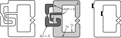
Figure 1. The knot $6_{3}$ (left). A negative special annulus presentation $(A,b)$ of $6_{3}$ (center). For simplicity, we often draw the attaching regions for the band by bold arcs and the bands are omitted (right).

Remark 2.2.

A knot $K$ has an annulus presentation if and only if the mirror image $\overline{K}$ has an annulus presentation. This fact is implicitly used in Section 7.

2.2. Annulus twist along an annulus presentation

Let $K$ be a knot with an annulus presentation $(A,b)$, which may not be special. We order the two components of the boundary $\partial A$, and set $\partial A=c_{1}\cup c_{2}$ with a parallel orientation. Then we can find a “shrunken” annulus $A^{\prime}\subset A$ with (ordered) boundary $\partial A^{\prime}=c^{\prime}_{1}\cup c^{\prime}_{2}$ which satisfies the following:

• The closure of ${A\setminus A^{\prime}}$, denoted by $\overline{A\setminus A^{\prime}}$, is a disjoint union of two annuli,

• each $c^{\prime}_{i}$ ($i=1,2$) is isotopic to $c_{i}$ in $\overline{A\setminus A^{\prime}}$, and

• $A\setminus(\partial A\cup A^{\prime})$ does not intersect $b(I\times I)$.

The left picture in Figure 2 will help us to understand the definition of $A^{\prime}$. Using the embedded annulus $A^{\prime}$, we define as follows:

Definition 2.3.

Let $n$ be an integer. The $n$-fold annulus twist along $(A,b)$ is to apply $(lk(c_{1},c_{2})+1/n)$-surgery on $c^{\prime}_{1}$ and $(lk(c_{1},c_{2})-1/n)$-surgery on $c^{\prime}_{2}$.

Note that the surgered 3-manifold $M_{c^{\prime}_{1}\cup c^{\prime}_{2}}(lk(c_{1},c_{2})+1/n,lk(c_{1},c_{2})-1/n)$ is homeomorphic to $\mathbf{S}^{3}$, see [20, Theorem 2.1]. Since $(c^{\prime}_{1}\cup c^{\prime}_{2})\cap K=\emptyset$, for a given integer $n$, we obtain a new knot $A^{n}(K)$ from $K$ by the $n$-fold annulus twist along $(A,b)$. We call $A^{n}(K)$ the knot obtained from $K$ by the $n$-fold annulus twist along $(A,b)$. The knot $A^{1}(K)$ is called the knot obtained from $K$ by the annulus twist along $(A,b)$ and we denote it by $A(K)$.

Example 2.4.

Let $(A,b)$ be the special annulus presentation of $6_{3}$ given in Figure 1. Then $A(6_{3})$ is the knot in Figure 2 (center and right).

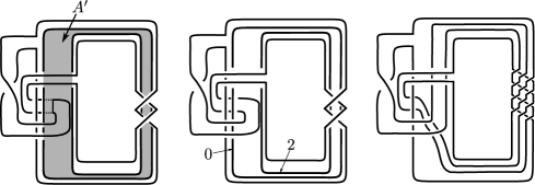
Figure 2. A shrunken annulus $A^{\prime}$ (left), $A(6_{3})$ in the surgered 3-manifold $M_{c^{\prime}_{1}\cup c^{\prime}_{2}}(2,0)$ (center) and $A(6_{3})$ in $\mathbf{S}^{3}$ (right)

The following is essentially due to Osoinach [20, Theorem 2.3] (see also [26]).

Theorem 2.5.

Let $K\subset\mathbf{S}^{3}$ be a knot with an annulus presentation $(A,b)$, which may not be special. Then, there is an orientation-preservingly homeomorphism $\phi_{n}\colon M_{K}(0)\rightarrow M_{A^{n}(K)}(0)$ for any $n\in\mathbf{Z}$. In particular, $\phi_{n}$ is given as in Figure 3.

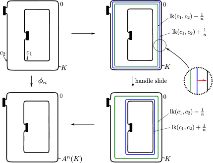
Figure 3. (color online) The definition of the $n$-th Osoinach-Teragaito’s homeomorphism $\phi_{n}$

We call $\phi_{n}$ the $n$-th Osoinach-Teragaito’s homeomorphism since Osoinach [20] introduced the homeomorphism $\phi_{n}$ and Teragaito [26] gave a surgery description of $\phi_{n}$. We simply call $\phi_{1}$ Osoinach-Teragaito’s homeomorphism and denote it by $\phi$.

Example 2.6.

We have $M_{6_{3}}(0)\cong M_{A^{n}(6_{3})}(0)$ for any integer $n$ by Theorem 2.5.

3. Proof of Theorem 1.3

The first author, Jong, Luecke and Osoinach [2, Section 3.1.2] introduced the operation $(\ast m)$ to construct infinitely many distinct knots with the same $m$-surgery. In this section, we recall the definition of the operation $(\ast m)$ and highlight a property of the operation $(\ast m)$. As an application, we prove Theorem 1.3, which states that $6_{3}$ has infinitely many non-characterizing slopes.

Let $K$ be a knot with a special annulus presentation $(A,b)$. We define the operation $(\ast m)$ as follows: Let $A(K)$ be the knot obtained from $K$ by the annulus twist along $(A,b)$, and $\gamma_{A(K)}$ a curve in $\mathbf{S}^{3}\setminus\nu(A(K))$ depicted in Figure 4.

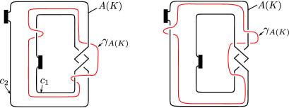
Figure 4. (color online) The definition of the curve $\gamma_{A(K)}$

Note that the definition of $\gamma_{A(K)}$ depends on the twist of $A$. We denote by $T_{m}(A(K))$ the knot obtained from $A(K)$ by twisting $m$ times along $\gamma_{A(K)}$. The operation $K\mapsto T_{m}(A(K))$ is called the operation $(\ast m)$. The most important property of the operation $(\ast m)$ is the following.

Theorem 3.1 ([2, Theorem 3.7]).

Let $K$ be a knot with a special annulus presentation $(A,b)$. Then, there is an orientation-preservingly homeomorphism $\psi_{m}\colon M_{K}(m)\rightarrow M_{T_{m}(A(K))}(m)$.

In [2, Figure 15], we find a proof of Theorem 3.1 for the case where $A$ is the negative Hopf band. For the reader’s convenience, in Appendix, we give a complete proof of Theorem 3.1.

Remark 3.2.

In Theorem 3.1, we cannot remove the assumption that an annulus presentation $(A,b)$ is special. If the annulus $A$ is knotted, then the corresponding curve $\gamma_{A(K)}$ will be knotted. Even if the annulus $A$ is unknotted, if $A$ is not Hopf bands, the corresponding slope of the curve $\gamma_{A(K)}$ will not be $-\dfrac{1}{m}$.

Now we are ready to prove Theorem 1.3.

Proof of Theorem 1.3.

Let $(A,b)$ be the special annulus presentation of $6_{3}$ given in Figure 1. By Theorem 3.1, we have $M_{6_{3}}(m)\cong M_{T_{m}(A(6_{3}))}(m)$. All we have to prove is that

$$6_{3}\neq T_{m}(A(6_{3}))$$

for infinitely many integers $m$. By [2, Lemma 3.12], we have $\Delta_{6_{3}}(t)\neq\Delta_{T_{m}(A(6_{3}))}(t)$ for any positive integer $m$, where $\Delta_{K}(t)$ is the Alexander polynomial of a knot $K$. This implies that $6_{3}\neq T_{m}(A(6_{3}))$ for infinitely many integers $m$, that is, $6_{3}$ has infinitely many non-characterizing slopes. ∎

4. Baker-Motegi’s condition on non-characterizing slopes

In [4], Baker and Motegi gave a sufficient condition for a given knot to have infinitely many non-characterizing slopes. In this section, we show that a knot which has a special annulus presentation with some property satisfies Baker-Motegi’s condition.

It seems to be convenient to introduce the following terminology.

Definition 4.1.

A knot $K\subset\mathbf{S}^{3}$ satisfies Baker-Motegi’s condition (BM-condition for short) if we can take an unknot $c$ disjoint from $K$ which satisfies the following properties:

• $c$ is not a meridian of $K$, and

• the $(0,0)$-surgery on $K\cup c$ yields $\mathbf{S}^{3}$.

Under this terminology, Baker and Motegi proved the following theorem.

Theorem 4.2.

$($[4, Theorem 1.3]$)$ Any knot with BM-condition has infinitely many non-characterizing slopes.

Remark 4.3.

The technique used in [4] is essentially the same as use of a dualizable pattern defined by Gompf-Miyazaki [6] and developed by Miller and Piccirillo [18].

Baker and Motegi asked which knots satisfy BM-condition, see [4, Question 5.3]. They proved that any L-space knot does not satisfy BM-condition, which is a “negative” result ([4, Theorem 1.8]). The following lemma gives a constructive result.

Lemma 4.4.

Let $K$ be a knot with a special annulus presentation $(A,b)$ and $\beta_{K}\subset\mathbf{S}^{3}\setminus\nu(K)$ the closed curve depicted in Figure 5. Then the $(0,0)$-surgery on $K\cup\beta_{K}$ yields $\mathbf{S}^{3}$. Moreover, if $\beta_{K}$ is not a meridian of $K$ in $\mathbf{S}^{3}$, then $K$ satisfies BM-condition.

Proof.

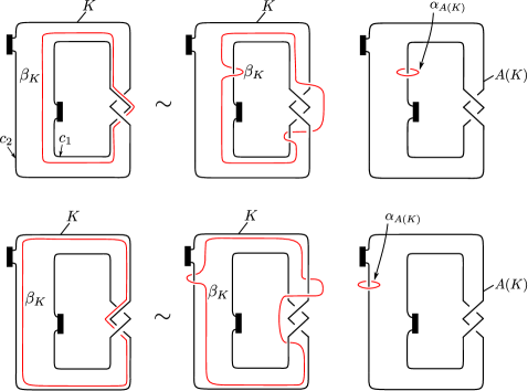
Figure 5. (color online) The definition of the closed curve $\beta_{K}\subset\mathbf{S}^{3}\setminus\nu(K)$

Let $L\subset M_{K}(0)$ be the surgery dual to $K$. We can regard $\beta_{K}$ as a knot in $M_{K}(0)$ because of $\beta_{K}\subset\mathbf{S}^{3}\setminus\nu(K)=M_{K}(0)\setminus\nu(L)$. Then, we can check that Osoinach-Teragaito’s homeomorphism $\phi$ induces a homeomorphism

$$\phi\colon(M_{K}(0),\beta_{K})\rightarrow(M_{A(K)}(0),\alpha_{A(K)}),$$

where $\alpha_{A(K)}$ is a meridian of $A(K)$. Moreover, we see that $\phi$ preserves slopes of $\beta_{K}$ and $\alpha_{A(K)}$. Since $M_{A(K)\cup\alpha_{A(K)}}(0,0)\cong\mathbf{S}^{3}$, we have $M_{K\cup\beta_{K}}(0,0)\cong\mathbf{S}^{3}$. Moreover, if $\beta_{K}$ is not a meridian of $K$, we see that $K$ satisfies BM-condition by taking $c=\beta_{K}$ in the definition of BM-condition. ∎

Remark 4.5.

There is an alternative proof of Theorem 1.3. By applying Lemma 4.4 to the special annulus presentation of $6_{3}$ depicted in Figure 1, we see that $6_{3}$ has infinitely many non-characterizing slopes. For the detail, see the next section. In the forthcoming paper, we prove that the two proofs of Theorem 1.3 are essentially the same.

5. Proof of Theorem 1.4

In this section, we prove Theorem 1.4, which states that the knots $6_{2}$, $6_{3}$, $7_{6}$, $7_{7}$, $8_{1}$, $8_{3}$, $8_{4}$, $8_{6}$, $8_{7}$, $8_{9}$, $8_{10}$, $8_{11}$, $8_{12}$, $8_{13}$, $8_{14}$, $8_{17}$, $8_{20}$ and $8_{21}$ have infinitely many non-characterizing slopes.

The following lemma is useful in finding a special annulus presentation of a given knot.

Lemma 5.1.

$($[1, Lemma 2.2]$)$ Any unknotting number one knot has a special annulus presentation.

Remark 5.2.

The unknotting number of the Conway knot is one. In [22], Piccirillo used Lemma 5.1 implicitly, see Figure 6 (compare with (d) in Figure 4 in [22]).

Figure 6. A special annulus presentation $(A,b)$ of the Conway knot

We obtain the following.

Lemma 5.3.

The following knots have special annulus presentations: $U$, $3_{1}$, $4_{1}$, $5_{2}$, $6_{1}$, $6_{2}$, $6_{3}$, $7_{2}$, $7_{6}$, $7_{7}$, $8_{1}$, $8_{3}$, $8_{4}$, $8_{6}$, $8_{7}$, $8_{9}$, $8_{10}$, $8_{11}$, $8_{12}$, $8_{13}$, $8_{14}$, $8_{17}$, $8_{20}$, $8_{21}$.

Proof.

The unknotting number of $U$, $3_{1}$, $4_{1}$, $5_{2}$, $6_{1}$, $6_{2}$, $6_{3}$, $7_{2}$, $7_{6}$, $7_{7}$, $8_{1}$, $8_{7}$, $8_{9}$, $8_{11}$, $8_{13}$, $8_{14}$, $8_{17}$, $8_{20}$ and $8_{21}$ is one. By Lemma 5.1, these knots have special annulus presentations. The unknotting number of $8_{3},8_{4},8_{6},8_{10}$ and $8_{12}$ is two. We can find special annulus presentations for these knots, see Figure 7. ∎

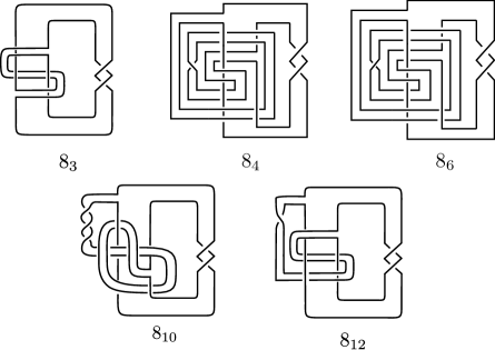
Figure 7. Special annulus presentations of $8_{3}$, $8_{4}$, $8_{6}$, $8_{10}$ and $8_{12}$

The following lemma is a key to prove Theorem 1.4.

Lemma 5.4.

The knots $6_{2}$, $6_{3}$, $7_{6}$, $7_{7}$, $8_{1}$, $8_{3}$, $8_{4}$, $8_{6}$, $8_{7}$, $8_{9}$, $8_{10}$, $8_{11}$, $8_{12}$, $8_{13}$, $8_{14}$, $8_{17}$, $8_{20}$ and $8_{21}$ satisfy BM-condition.

Proof.

Let $\kappa$ be a knot with a special annulus presentation. We denote by $\alpha_{\kappa}$ a meridian of $\kappa$ and by $\beta_{\kappa}$ the closed curve defined in Figure 5. We first consider $6_{2}$. It has a special annulus presentation and the link $6_{2}\cup\beta_{6_{2}}$ is the left picture in Figure 8. Then we have

$$\nabla_{6_{2}\cup\alpha_{6_{2}}}(z)=-z^{5}-z^{3}+z,\ \ \ \ \nabla_{6_{2}\cup\beta_{6_{2}}}(z)=-z^{3}+z,$$

where we choose orientations of $6_{2}\cup\alpha_{6_{2}}$ and $6_{2}\cup\beta_{6_{2}}$ so that the linking numbers of $6_{2}\cup\alpha_{6_{2}}$ and $6_{2}\cup\beta_{6_{2}}$ are one, respectively. Here $\nabla_{L}(z)$ is the Conway polynomial of an oriented link $L$. Therefore $\beta_{6_{2}}$ is not a meridian of $6_{2}$. This implies that $6_{2}$ satisfies BM-condition by Lemma 4.4.

Let $K$ be one of the knots $6_{3}$, $7_{6}$, $7_{7}$, $8_{1}$, $8_{3}$, $8_{4}$, $8_{6}$, $8_{7}$, $8_{9}$, $8_{10}$, $8_{11}$, $8_{12}$, $8_{13}$, $8_{14}$, $8_{17}$, $8_{20}$ and $8_{21}$. It has a special annulus presentation and the link $K\cup\beta_{K}$ is as in Figures 8 and 9. Then we have $\nabla_{K\cup\alpha_{K}}(z)\neq\nabla_{K\cup\beta_{K}}(z)$, where we choose orientations of $K\cup\alpha_{K}$ and $K\cup\beta_{K}$ so that their linking numbers are one. Therefore $\beta_{K}$ is not a meridian of $K$. This implies that $K$ satisfies BM-condition by Lemma 4.4. For the actual calculations, see the following.

$$\nabla_{6_{3}\cup\alpha_{6_{3}}}(z) =z^{5}+z^{3}+z, \nabla_{6_{3}\cup\beta_{6_{3}}}(z) =z^{3}+z,$$

$$\nabla_{7_{6}\cup\alpha_{7_{6}}}(z) =-z^{5}+z^{3}+z, \nabla_{7_{6}\cup\beta_{7_{6}}}(z) =z^{3}+z,$$

$$\nabla_{7_{7}\cup\alpha_{7_{7}}}(z) =z^{5}-z^{3}+z, \nabla_{7_{7}\cup\beta_{7_{7}}}(z) =-z^{3}+z,$$

$$\nabla_{8_{1}\cup\alpha_{8_{1}}}(z) =-3z^{3}+z, \nabla_{8_{1}\cup\beta_{8_{1}}}(z) =-z^{5}-3z^{3}+z,$$

$$\nabla_{8_{3}\cup\alpha_{8_{3}}}(z) =-4z^{3}+z, \nabla_{8_{3}\cup\beta_{8_{3}}}(z) =-z^{5}-4z^{3}+z,$$

$$\nabla_{8_{4}\cup\alpha_{8_{4}}}(z) =-2z^{5}-3z^{3}+z, \nabla_{8_{4}\cup\beta_{8_{4}}}(z) =-z^{5}-3z^{3}+z,$$

$$\nabla_{8_{6}\cup\alpha_{8_{6}}}(z) =-2z^{5}-2z^{3}+z, \nabla_{8_{6}\cup\beta_{8_{6}}}(z) =-z^{5}-2z^{3}+z,$$

$$\nabla_{8_{7}\cup\alpha_{8_{7}}}(z) =z^{7}+3z^{5}+2z^{3}+z, \nabla_{8_{7}\cup\beta_{8_{7}}}(z) =2z^{3}+z,$$

$$\nabla_{8_{9}\cup\alpha_{8_{9}}}(z) =-z^{7}-3z^{5}-2z^{3}+z, \nabla_{8_{9}\cup\beta_{8_{9}}}(z) =-2z^{3}+z,$$

$$\nabla_{8_{10}\cup\alpha_{8_{10}}}(z) =z^{7}+3z^{5}+3z^{3}+z, \nabla_{8_{10}\cup\beta_{8_{10}}}(z) =3z^{3}+z,$$

$$\nabla_{8_{11}\cup\alpha_{8_{11}}}(z) =-2z^{5}-z^{3}+z, \nabla_{8_{11}\cup\beta_{8_{11}}}(z) =-z^{3}+z,$$

$$\nabla_{8_{12}\cup\alpha_{8_{12}}}(z) =z^{5}-3z^{3}+z, \nabla_{8_{12}\cup\beta_{8_{12}}}(z) =z^{7}+3z^{5}-3z^{3}+z,$$

$$\nabla_{8_{13}\cup\alpha_{8_{13}}}(z) =2z^{5}+z^{3}+z, \nabla_{8_{13}\cup\beta_{8_{13}}}(z) =z^{3}+z,$$

$$\nabla_{8_{14}\cup\alpha_{8_{14}}}(z) =-2z^{5}+z, \nabla_{8_{14}\cup\beta_{8_{14}}}(z) =z,$$

$$\nabla_{8_{17}\cup\alpha_{8_{17}}}(z) =-z^{7}-2z^{5}-z^{3}+z, \nabla_{8_{17}\cup\beta_{8_{17}}}(z) =-z^{3}+z,$$

$$\nabla_{8_{20}\cup\alpha_{8_{20}}}(z) =z^{5}+2z^{3}+z, \nabla_{8_{20}\cup\beta_{8_{20}}}(z) =2z^{3}+z,$$

$$\nabla_{8_{21}\cup\alpha_{8_{21}}}(z) =-z^{5}-3z^{3}+z, \nabla_{8_{21}\cup\beta_{8_{21}}}(z) =-3z^{3}+z.$$

∎

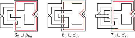
Figure 8. (color online) 2-component links $6_{2}\cup\beta_{6_{2}}$, $6_{3}\cup\beta_{6_{3}}$ and $7_{6}\cup\beta_{7_{6}}$

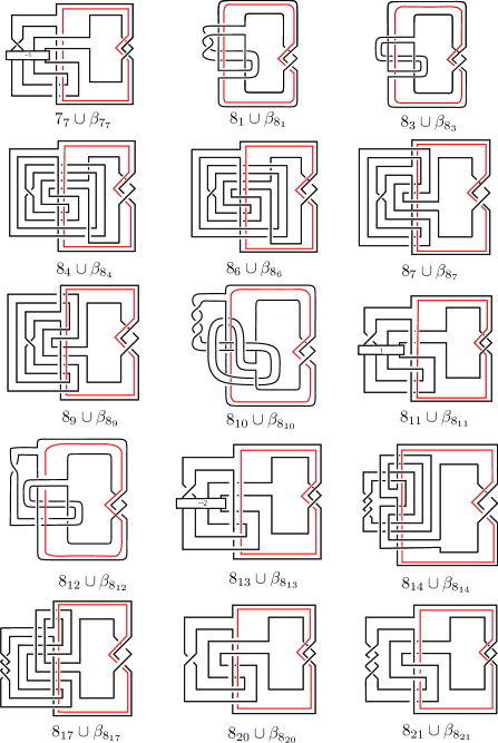
Figure 9. (color online) 2-component links $7_{7}\cup\beta_{7_{7}}$, $8_{1}\cup\beta_{8_{1}}$, $8_{3}\cup\beta_{8_{3}}$, $8_{4}\cup\beta_{8_{4}}$, $8_{6}\cup\beta_{8_{6}}$, $8_{7}\cup\beta_{8_{7}}$, $8_{9}\cup\beta_{8_{9}}$, $8_{10}\cup\beta_{8_{10}}$, $8_{11}\cup\beta_{8_{11}}$, $8_{12}\cup\beta_{8_{12}}$, $8_{13}\cup\beta_{8_{13}}$, $8_{14}\cup\beta_{8_{14}}$, $8_{17}\cup\beta_{8_{17}}$, $8_{20}\cup\beta_{8_{20}}$ and $8_{21}\cup\beta_{8_{21}}$.

We are ready to prove Theorem 1.4.

Proof of Theorem 1.4.

By Lemma 5.4, the knots $6_{2}$, $6_{3}$, $7_{6}$, $7_{7}$, $8_{1}$, $8_{3}$, $8_{4}$, $8_{6}$, $8_{7}$, $8_{9}$, $8_{10}$, $8_{11}$, $8_{12}$, $8_{13}$, $8_{14}$, $8_{17}$, $8_{20}$ and $8_{21}$ satisfy BM-condition. Therefore, these knots have infinitely many non-characterizing slopes by Theorem 4.2. ∎

6. Triviality of annulus twists and application to knot theory

In this section, we introduce the notion of trivial annulus twists and investigate a sufficient condition for an annulus twist to be trivial. As a byproduct, we obtain a new method to construct equivalent knots in a 3-manifold which might be non-isotopic. Throughout this section, we only consider $0$-surgery on knots.

6.1. Triviality of the $n$-fold annulus twist

We introduce the notion of “trivial” for the $n$-fold annulus twist along an annulus presentation.

Let $K$ be a knot with an annulus presentation $(A,b)$ and $A^{n}(K)$ the knot as in Section 2.2. We denote by $\alpha_{A^{n}(K)}\subset\mathbf{S}^{3}$ a meridian of $A^{n}(K)$ and by $L_{A^{n}(K)}$ the surgery dual to $A^{n}(K)$ in $M_{A^{n}(K)}(0)$. We can regard $\alpha_{A^{n}(K)}$ as a curve in $M_{A^{n}(K)}(0)$ since we have

$$\alpha_{A^{n}(K)}\subset\mathbf{S}^{3}\setminus\nu(A^{n}(K))=M_{A^{n}(K)}(0)\setminus\nu(L_{A^{n}(K)}).$$

Definition 6.1.

The $n$-fold annulus twist along $(A,b)$ is trivial if $\phi_{n}(\alpha_{K})$ is isotopic to $\alpha_{A^{n}(K)}$ in $M_{A^{n}(K)}(0)$, where $\phi_{n}\colon M_{K}(0)\rightarrow M_{A^{n}(K)}(0)$ is the $n$-th Osoinach-Teragaito’s homeomorphism.

The following lemma justifies the above definition.

Lemma 6.2.

Let $K$ be a knot with an annulus presentation $(A,b)$. Suppose that the $n$-fold annulus twist along $(A,b)$ is trivial. Then we obtain $K=A^{n}(K)$.

Proof.

Since the $n$-fold annulus twist along $(A,b)$ is trivial, $\phi_{n}(\alpha_{K})$ is isotopic to $\alpha_{A^{n}(K)}$ in $M_{A^{n}(K)}(0)$. Note that $\alpha_{A^{n}(K)}$ is isotopic to $L_{A^{n}(K)}$ in $M_{A^{n}(K)}(0)$. Hence, we have

$$\mathbf{S}^{3}\setminus\nu(K) =M_{K}(0)\setminus\nu(L_{K})$$

$$\cong M_{K}(0)\setminus\nu(\alpha_{K})$$

$$\cong\phi_{n}(M_{K}(0))\setminus\phi_{n}(\nu(\alpha_{K}))$$

$$\cong M_{A^{n}(K)}(0)\setminus\nu(\alpha_{A^{n}(K)})$$

$$\cong M_{A^{n}(K)}(0)\setminus\nu(L_{A^{n}(K)})$$

$$=\mathbf{S}^{3}\setminus\nu(A^{n}(K)).$$

By the Knot Complement Theorem [8], we obtain $K=A^{n}(K)$. ∎

The following lemma gives us many examples of trivial annulus twists.

Lemma 6.3.

Let $K$ be a knot with a special annulus presentation $(A,b)$. Suppose that there is some disk $D$ such that $\partial D=c_{1}$ and $\operatorname{Int}D\cap b=\emptyset$ (see Figure 10). Then, we obtain the following.

• If $(A,b)$ is negative, the $(-1)$-fold annulus twist along $(A,b)$ is trivial.

• If $(A,b)$ is positive, the $(+1)$-fold annulus twist along $(A,b)$ is trivial.

Proof.

We can assume that $\operatorname{Int}D\cap K$ consists of a single point as in Figure 10. Suppose that $(A,b)$ is negative. Then, $(\phi_{-1})^{-1}\colon M_{A^{-1}(K)}(0)\rightarrow M_{K}(0)$ sends $\alpha_{A^{-1}(K)}$ to $\alpha_{K}$ (see Figure 11). Indeed, by a small isotopy, $(\phi_{-1})^{-1}(\alpha_{A^{-1}(K)})$ is isotopic to a curve $\ell\subset D$ and it is isotopic to $\alpha_{K}$ since we can find an annulus bounded by the curve $\ell$ and $\alpha_{K}$ by using the given disk $D$. In the case where $(A,b)$ is positive, we can prove that the $(+1)$-fold annulus twist along $(A,b)$ is trivial similarly. ∎

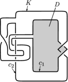
Figure 10. A disk $D$ satisfying $\partial D=c_{1}$ and $\operatorname{Int}D\cap b=\emptyset$

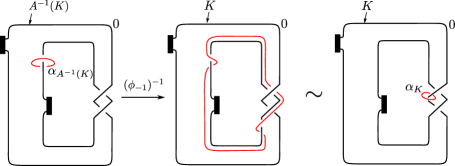
Figure 11. (color online) Proof of Lemma 6.3

As a corollary of Lemma 6.3, we obtain the following, which gives an alternative proof of [25, Theorem 5.1] for the unoriented case.

Corollary 6.4 (e.g. [25, Theorem 5.1]).

Let $K$ be a knot with a special annulus presentation $(A,b)$. Suppose that there is some disk $D$ such that $\partial D=c_{1}$ and $\operatorname{Int}D\cap b=\emptyset$ (see Figure 10). Then, we obtain the following.

• If $(A,b)$ is negative, then $K=A^{-1}(K)$.

• If $(A,b)$ is positive, then $K=A^{+1}(K)$.

Example 6.5.

Let $(A,b)$ be the special annulus presentation of $6_{3}$ as in Figure 1. Then we have $6_{3}=A^{-1}(6_{3})$ by Corollary 6.4.

6.2. Equivalent knots in a 3-manifold which might be non-isotopic

In this subsection, we consider whether the converse of Lemma 6.2 holds or not, which motivates the following question.

Question 6.6.

Let $K$ be a knot with an annulus presentation $(A,b)$. Fix an integer $n$. If we have $K=A^{n}(K)$, is the $n$-fold annulus twist along $(A,b)$ trivial? More strongly, is the $n$-th Osoinach-Teragaito’s homeomorphism

$$\phi_{n}\colon M_{K}(0)\rightarrow M_{A^{n}(K)}(0)=M_{K}(0)$$

is isotopic to the identity?

We do not have any counterexamples to this question at the time of writing. Potential counterexamples are constructed as follows: Let $K$ be a knot with an annulus presentation $(A,b)$. Suppose that $\operatorname{Int}A\cap b=\emptyset$. Then, for any integer $n$, we have $K=A^{n}(K)$. However, we do not know whether the $n$-fold annulus twist along $(A,b)$ is trivial or not. For example, the knot $8_{1}$ has such an annulus presentation, see Figure 12. If the $n$-fold annulus twist along the annulus presentation are not trivial, then the two knots $\alpha_{8_{1}}$ and $\phi(\alpha_{8_{1}})$ in $M_{8_{1}}(0)$ are not isotopic although they are equivalent.

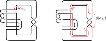
Figure 12. (color online) Equivalent knots $\alpha_{8_{1}}$ and $\phi(\alpha_{8_{1}})$ in the 3-manifold $M_{8_{1}}(0)$

7. Tabulation of annulus presentations of knots

In Section 5, we proved that some knots up to 8-crossings have special annulus presentations (see Lemma 5.3). In this section, we give four obstructions for knots to have (special) annulus presentations. As an application, we prove the following.

Theorem 7.1.

The following knots do not have special annulus presentations:

$$5_{1},\ 7_{1},\ 7_{3},\ 7_{4},\ 7_{5},\ 8_{2},\ 8_{5},\ 8_{8},\ 8_{15},\ 8_{16},\ 8_{18},\ 8_{19}.$$

As a summary, we obtain Table 1. Here

• “$u=1$” means an unknotting number one knot and it has a special annulus presentation by Lemma 5.1.

• “Yes” means a knot of unknotting number $2$ and with a special annulus presentation (see Figure 7).

• “No” means a knot without any special annulus presentations by Theorem 7.1.

knot	special annulus presentation	knot	special annulus presentation
$3_{1}$	$u=1$	$8_{5}$	No
$4_{1}$	$u=1$	$8_{6}$	Yes
$5_{1}$	No	$8_{7}$	$u=1$
$5_{2}$	$u=1$	$8_{8}$	No
$6_{1}$	$u=1$	$8_{9}$	$u=1$
$6_{2}$	$u=1$	$8_{10}$	Yes
$6_{3}$	$u=1$	$8_{11}$	$u=1$
$7_{1}$	No	$8_{12}$	Yes
$7_{2}$	$u=1$	$8_{13}$	$u=1$
$7_{3}$	No	$8_{14}$	$u=1$
$7_{4}$	No	$8_{15}$	No
$7_{5}$	No	$8_{16}$	No
$7_{6}$	$u=1$	$8_{17}$	$u=1$
$7_{7}$	$u=1$	$8_{18}$	No
$8_{1}$	$u=1$	$8_{19}$	No
$8_{2}$	No	$8_{20}$	$u=1$
$8_{3}$	Yes	$8_{21}$	$u=1$
$8_{4}$	Yes	-	-

Table 1. List of prime knots with/without special annulus presentations

In Table $1$, we only consider whether a prime knot up to 8-crossings has a special annulus presentation or not. In general, a given knot has many special annulus presentations. In Section 7.5, we consider when we should regard two special annulus presentations as the same annulus presentation. We introduce the notion of equivalent annulus presentations.

7.1. The 4-ball genus obstruction

The following theorem implies that the 4-ball genus is an obstruction for knots to have annulus presentations.

Theorem 7.2.

Let $K$ be a knot. If $K$ has an annulus presentation, then the $4$-ball genus of $K$, denoted by $g_{4}(K)$, is less than or equal to one.

Proof.

Suppose that $(A,b)$ is an annulus presentation of $K$. Then, a single band surgery along the cocore of the band $b$ changes $K$ into $\partial A$. Hence, $K$ bounds an orientable proper surface of genus $1$ in $\mathbf{B}^{4}$. This means that $g_{4}(K)\leq 1$. ∎

Corollary 7.3.

The following knots do not have any annulus presentations:

$$5_{1},\ 7_{1},\ 7_{3},\ 7_{5},\ 8_{2},\ 8_{5},\ 8_{15},\ 8_{19}.$$

Proof.

Let $K$ be one of the above knots. Then $g_{4}(K)>1$, see KnotInfo [15]. By Theorem 7.2, $K$ does not have any annulus presentations. ∎

In general, it is a subtle question whether a knot $K$ with $g_{4}(K)\leq 1$ has (special) annulus presentations or not.

7.2. The concordance obstruction

Let $\nu$ be an integer-valued concordance invariant of oriented links satisfying

$$|\nu(L)-\nu(L^{\prime})|\leq-\chi(S)\ \text{and}\ \nu(H_{\pm})=\pm 1,$$

where $S$ is a concordance between two links $L$ and $L^{\prime}$, and $H_{+}$ (resp. $H_{-}$) is the positive (resp. negative) Hopf link. For example, the Rasmussen invariant $s$ satisfies this condition, and we will use this invariant in the proof of Corollary 7.7. The following theorem implies that $\nu$ is an obstruction for knots to have (negative) special annulus presentations.

Theorem 7.4.

Let $K$ be an oriented knot. If $K$ has a negative special annulus presentation, then

$$-2\leq\nu(K)\leq 0.$$

In particular, if $\nu(K)=2$, then $K$ does not have any negative special annulus presentations.

Proof.

Suppose that $K$ has a negative special annulus presentation. Then, by the definition, $K$ is obtained from the negative Hopf link by a single band surgery. Hence, we have

$$|\nu(K)-\nu(H_{-})|=|\nu(K)+1|\leq 1.$$

That is, $-2\leq\nu(K)\leq 0$. ∎

7.3. The Jones polynomial obstruction

The Jones polynomial $V_{L}(t)$ is a Laurent polynomial invariant of an oriented link $L\subset\mathbf{S}^{3}$ which is characterized by

(1) $$V_{U}(t) =1,$$

(2) $$t^{-1}V_{L_{+}}(t)-tV_{L_{-}}(t) =(t^{1/2}-t^{-1/2})V_{L_{0}}(t),$$

where the links $L_{+}$, $L_{-}$, $L_{0}$ are identical except for a neighborhood of a point as shown in Figure 13, for example, see [10].

Figure 13. A skein triple

The equation (2) is called Jones’s skein relation. It is well known that the value of $V_{L}(t)$ at a root of unity is related to topological properties of $L$. Let $\omega=e^{\frac{\pi i}{3}}$ be the 6th root of unity (not the cube root of unity). Lickorish and Millett [14] described the values of the Jones polynomial $V_{L}(t)$ at $\omega$ as follows:

Theorem 7.5.

Let $L$ be an oriented link in $\mathbf{S}^{3}$, $c$ the number of components of $L$, and $d$ the dimension of $H_{1}(\Sigma(L),\mathbf{Z}/\mathbf{3Z})$, where $\Sigma(L)$ is the double cover of $\mathbf{S}^{3}$ branched along $L$. Then

$$V_{L}(\omega)=\pm i^{c-1}(i\sqrt{3})^{d}.$$

Theorems 7.6 and 7.8 imply that the Jones polynomial is an obstruction for knots to have (positive) special annulus presentations.

Theorem 7.6.

Let $K$ be a knot with $V_{K}(\omega)=-i\sqrt{3}$. Then $K$ does not have any positive special annulus presentations.

Note that Theorem 7.6 is a special case of a more general result in [9, Theorem 2.2]. Here we give a direct proof of Theorem 7.6 for the sake of the reader.

Proof.

Suppose that $K$ has a positive special annulus presentation. Then we can suppose that the positive Hopf link $H_{+}$ is obtained from $K$ by a single band surgery as in Figure 14.

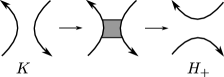
Figure 14. A band surgery

Here we consider the skein triple in Figure 15.

Figure 15. A skein triple

Jones’s skein relation implies that

$$t^{-1}V_{K}(t)-tV_{K^{\prime}}(t)=(t^{1/2}-t^{-1/2})V_{H_{+}}(t).$$

Since $V_{H_{+}}(t)=-t^{5/2}-t^{1/2}$, this means that $V_{K^{\prime}}(t)=t^{-2}V_{K}(t)-t^{-1}+1-t+t^{2}$. Hence, we have

$$V_{K^{\prime}}(\omega) =\omega^{-2}V_{K}(\omega)-\omega^{-1}+1-\omega+\omega^{2}$$

$$=\left(-\frac{1}{2}-\frac{\sqrt{3}}{2}i\right)V_{K}(\omega)-\frac{1}{2}+\frac{\sqrt{3}}{2}i$$

$$=-2+\sqrt{3}i,$$

where we used, for the last equality, the hypothesis that $V_{K}(\omega)=-i\sqrt{3}$. This contradicts Theorem 7.5. Therefore $K$ does not have any positive special annulus presentations. ∎

Corollary 7.7.

The knot $7_{4}$ does not have any special annulus presentations.

Proof.

Let $K$ be the knot $7_{4}$ in Figure 16. Then we can calculate that $s(K)=2$. By Theorem 7.4, $K$ does not have any negative special annulus presentations. On the other hand, we have

$$V_{K}(t) =t-2t^{2}+3t^{3}-2t^{4}+3t^{5}-2t^{6}+t^{7}-t^{8}.$$

Therefore we obtain $V_{K}(\omega)=-i\sqrt{3}$. By Theorem 7.6, $K$ does not have any positive special annulus presentations. ∎

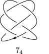
Figure 16. The knot $7_{4}$

Theorem 7.8.

Let $K$ be a knot with $V_{K}(\omega)=\pm 3$. Then $K$ does not have any special annulus presentations.

Proof.

Assume that $K$ has a positive special annulus presentation. Then, by the proof of Theorem 7.6, we have

$$V_{K^{\prime}}(\omega)=\left(-\frac{1}{2}-\frac{\sqrt{3}}{2}i\right)V_{K}(\omega)+\frac{\sqrt{3}}{2}i-\frac{1}{2}.$$

Both cases $V_{K}(\omega)=\pm 3$ contradict Theorem 7.5. Hence, $K$ does not have any positive special annulus presentations. Let $\overline{K}$ be the mirror image of $K$. Since $V_{\overline{K}}(\omega)=\overline{V_{K}(\omega)}=\pm 3$, we see that $\overline{K}$ also does not have any positive special annulus presentations. Equivalently, $K$ does not have any negative special annulus presentations. ∎

Corollary 7.9.

The knot $8_{18}$ does not have any special annulus presentations.

Proof.

We have $V_{8_{18}}(\omega)=\pm 3$. By Theorem 7.8, the knot $8_{18}$ does not have any negative special annulus presentations. ∎

7.4. The $Q$-polynomial obstruction

The $Q$-polynomial $Q_{L}(x)$ is a Laurent polynomial invariant of an unoriented link $L\subset\mathbf{S}^{3}$ which is characterized by

$$Q_{U}(x) =1,$$

$$Q_{L_{+}}(x)+Q_{L_{-}}(x) =x(Q_{L_{0}}(x)+Q_{L_{\infty}}(x)),$$

where the links $L_{+}$, $L_{-}$, $L_{0}$, $L_{\infty}$ are identical except for a neighborhood of a point as shown in Figure 17, for example, see [10].

Remark 7.10.

The $Q$-polynomial $Q_{L}(x)$ have the following properties:

• $Q_{L}(x)=F_{L}(1,x)$, where $F_{L}(a,z)$ is the Kauffman polynomial of $L$,

• $Q_{L}(x)=Q_{\overline{L}}(x)$, where $\overline{L}$ is the mirror image of $L$.

Figure 17. A skein quadruple

An analogous result of Theorem 7.6 holds for the Q-polynomial.

Theorem 7.11.

Let $K$ be a knot with a special annulus presentation. Then we have $Q_{L}\left(\dfrac{\sqrt{5}-1}{2}\right)\neq\sqrt{5}$.

Proof.

Based on the result of Long in [23] (see also Stoimenow [24]), Kanenobu [9, Theorem 3.1] proved that if two links $L_{1}$ and $L_{2}$ are related by a single band surgery, then

$$Q_{L_{1}}\left(\dfrac{\sqrt{5}-1}{2}\right)\Big{/}Q_{L_{2}}\left(\dfrac{\sqrt{5}-1}{2}\right)\in\{\pm 1,\sqrt{5}^{\pm 1}\}.$$

Since the knot $K$ and the Hopf link $H$ are related by a single band surgery, we obtain

$$Q_{K}\left(\dfrac{\sqrt{5}-1}{2}\right)\Big{/}Q_{H}\left(\dfrac{\sqrt{5}-1}{2}\right)\in\{\pm 1,\sqrt{5}^{\pm 1}\}.$$

Since $Q_{H}\left(\dfrac{\sqrt{5}-1}{2}\right)=-1$, this implies that $Q_{K}\left(\dfrac{\sqrt{5}-1}{2}\right)\in\{\pm 1,-\sqrt{5}^{\pm 1}\}$. In particular, $Q_{K}\left(\dfrac{\sqrt{5}-1}{2}\right)\neq\sqrt{5}$. ∎

Corollary 7.12.

The knots $8_{8}$ and $8_{16}$ do not have any special annulus presentations.

Proof.

We have the following.

$$Q_{8_{8}}(x) =1+4x+6x^{2}-10x^{3}-14x^{4}+4x^{5}+8x^{6}+2x^{7},$$

$$Q_{8_{16}}(x) =-3+10x+18x^{2}-22x^{3}-30x^{4}+8x^{5}+16x^{6}+4x^{7}.$$

Therefore

$$Q_{8_{8}}\left(\dfrac{\sqrt{5}-1}{2}\right)=Q_{8_{16}}\left(\dfrac{\sqrt{5}-1}{2}\right)=\sqrt{5}.$$

By Theorem 7.11, the knots $8_{8}$ and $8_{16}$ do not have any special annulus presentations. ∎

Proof of Theorem 7.1.

By Corollaries 7.3, 7.7, 7.9 and 7.12, the knots

$$5_{1},\ 7_{1},\ 7_{3},\ 7_{4},\ 7_{5},\ 8_{2},\ 8_{5},\ 8_{8},\ 8_{15},\ 8_{16},\ 8_{18},\ 8_{19}$$

do not have special annulus presentations. ∎

Remark 7.13.

There exist knots which have only non-special annulus presentations. By Theorem 7.1, the knots $7_{4}$, $8_{8}$, $8_{16}$ and $8_{18}$ do not have any special annulus presentations. On the other hand, it is easy to see that $7_{4}$ has a non-special annulus presentation (see Figure 18). Also, we can obtain a non-special annulus presentation of $8_{8}$ from a ribbon presentation of $8_{8}$. In fact, we can find a ribbon presentation of $8_{8}$ in [10, Appendix F.5], and this presentation is also a non-special annulus presentation of $8_{8}$. The authors do not know whether the knots $8_{16}$ and $8_{18}$ have non-special annulus presentations or not.

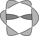
Figure 18. A non-special annulus presentation of $7_{4}$

7.5. Equivalent annulus presentations of knots

In general, a given knot has many special annulus presentations. For example, the knot $6_{3}$ has two special annulus presentations $(A,b_{1})$ and $(A,b_{2})$ as in Figure 19.

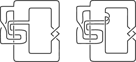
Figure 19. Two special annulus presentations of $6_{3}$

We define as follows.

Definition 7.14.

Let $(A_{i},b_{i})$ be an annulus presentation of a knot $K_{i}$ for $i=1,2$. Then $(A_{1},b_{1})$ and $(A_{2},b_{2})$ are equivalent if the $3$-component link $K_{1}\cup c_{1}^{\prime}\cup c_{2}^{\prime}$ is isotopic to $K_{2}\cup d_{1}^{\prime}\cup d_{2}^{\prime}$, where $K_{1}$ is deformed into $K_{2}$, and $A_{1}^{\prime}$, $A_{2}^{\prime}$ are the shrunken annuli corresponding to $(A_{1},b_{1})$, $(A_{2},b_{2})$ respectively and $\partial A_{1}^{\prime}=c_{1}^{\prime}\cup c_{2}^{\prime}$, $\partial A_{2}^{\prime}=d_{1}^{\prime}\cup d_{2}^{\prime}$.

The following theorem justifies the above definition.

Theorem 7.15.

Let $(A_{1},b_{1})$ and $(A_{2},b_{2})$ be equivalent annulus presentations of $K_{1}$ and $K_{2}$, respectively. Then we have

$$A_{1}^{n}(K_{1})=A_{2}^{n}(K_{2}),\text{or}\ A_{1}^{n}(K_{1})=A_{2}^{-n}(K_{2})$$

for any $n\in\mathbf{Z}$.

We omit the proof of Theorem 7.15 since it is immediately follows from Definition 7.14. The following lemma is useful to find equivalent annulus presentations.

Lemma 7.16.

Let $A$ be (possibly) twisted and knotted annulus in $\mathbf{S}^{3}$. Let $(A,b_{1})$ and $(A,b_{2})$ be two annulus presentations of a knot whose bands $b_{1}$ and $b_{2}$ are slightly different as in Figure 20. Then $(A,b_{1})$ and $(A,b_{2})$ are equivalent.

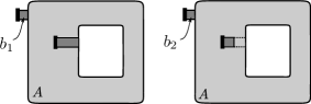
Figure 20. $A$ may be knotted and twisted.

Proof.

See Figure 21.

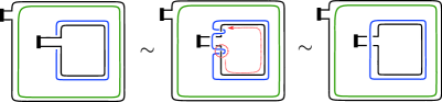
Figure 21. (color online) Proof of Lemma 7.16

∎

Example 7.17.

Two special annulus presentations $(A,b_{1})$ and $(A,b_{2})$ in Figure 19 are equivalent.

We do not know whether the converse of Theorem 7.15 holds or not.

Question 7.18.

Let $(A_{1},b_{1})$ and $(A_{2},b_{2})$ be annulus presentations of $K_{1}$ and $K_{2}$, respectively. If $A^{n}(K_{1})=A^{n}(K_{2})$ for any $n\in\mathbf{Z}$, then are $(A_{1},b_{1})$ and $(A_{2},b_{2})$ equivalent?

Acknowledgements. The final part of this paper was written in OIST. The first author thanks Andrew Lobb for inviting him to “Mini-Symposium : Knot Theory on Okinawa” during 17–21 February 2020. He also thanks Kazuhiro Ichihara for telling him the paper [5] and Chuck Livingston for clarifying some confusing points on orientations in Section 2. The authors thank the referee for his/her careful reading and helpful comments. The first author was supported by the Research Promotion Program for Acquiring Grants in-Aid for Scientific Research (KAKENHI) in Ritsumeikan University. The second author was supported by JSPS KAKENHI Grant number JP18K13416.

Appendix

We give a complete proof of Theorem 3.1.

Proof of Theorem 3.1.

A desired homeomorphism $\psi_{m}\colon M_{K}(m)\to M_{T_{m}(A(K))}(m)$ is given as in Figure 22 if $A$ is the negative Hopf band and as in Figure 23 if $A$ is the positive Hopf band. ∎

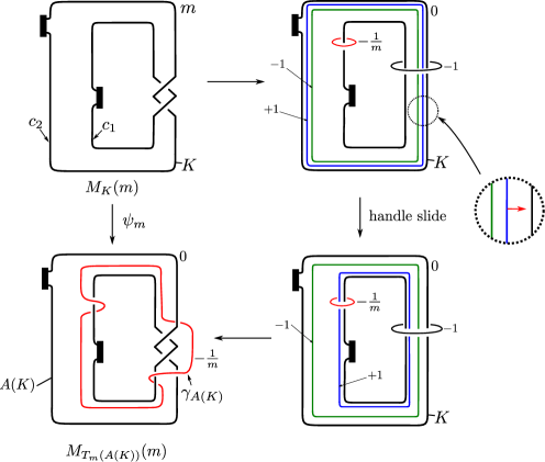
Figure 22. (color online) $\psi_{m}\colon M_{K}(m)\to M_{T_{m}(A(K))}(m)$ for the case where A is the negative Hopf band

Remark 7.19.

Note that $\psi_{m}$ in Figures 22 and 23 do not depend on the choices of the meridians with slopes $-1/m$ of $K$. For example, Figures 23 and 24 are essentially the same.

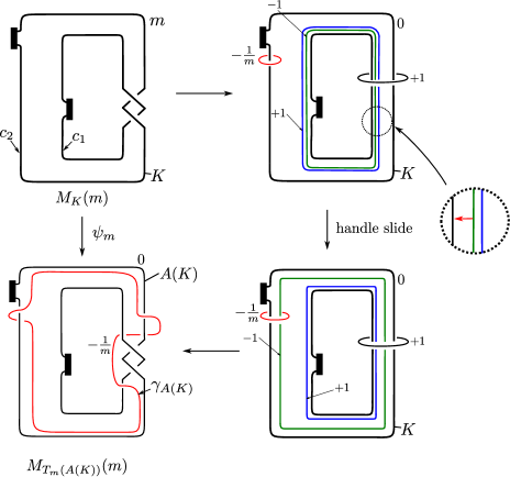
Figure 23. (color online) $\psi_{m}$ for the case where $A$ is the positive Hopf band

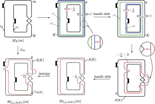
Figure 24. (color online)

References

- [1] T. Abe, I. Jong, Y. Omae, and M. Takeuchi, Annulus twist and diffeomorphic 4-manifolds, Math. Proc. Cambridge Philos. Soc. 155 (2013), 219–235.
- [2] T. Abe, I. Jong, J. Luecke, J. Osoinach, Infinitely many knots with the same integer surgery and a four-dimensional extension, Int. Math. Res. Not. IMRN 2015 (22), 11667–11693.
- [3] T. Abe and K. Tagami, Fibered knots with the same 0-surgery and the slice-ribbon conjecture, Math. Res. Lett. 23 (2016), 303–323.
- [4] K. Baker and K. Motegi, Non-characterizing slopes for hyperbolic knots, Algebr. Geom. Topol. 18, (2018), 1461-1480.
- [5] A. Cattabriga and E. Manfredi, Diffeomorphic vs Isotopic Links in Lens Spaces, Mediterranean Journal of Mathematics 15, Article number: 172 (2018).
- [6] R. E. Gompf and K. Miyazaki, Some well-disguised ribbon knots, Topology Appl. 64 (1995), 117–131.
- [7] C. Gordon, Some Aspects of Classical Knot Theory, (Proc. Sem., Plans-sur-Bex, 1977), Lecture Notes in Math. 685, Springer, Berlin, 1978, 1–60.
- [8] C. McA. Gordon and J. Luecke, Knots are determined by their complements, J. Amer. Math. Soc. 2 (1989), 371–415.
- [9] T. Kanenobu, Band surgery on knots and links, J. Knot Theory Ramifications 19 (2010), 1535–1547.
- [10] A. Kawauchi, A survey of knot theory, Birkhäuser Verlag, Basel, 1996.
- [11] P. Kronheimer, T. Mrowka, P. Ozsváth, and Z. Szabó, Monopoles and lens space surgeries, Ann. of Math. 165 (2007), 457–546.
- [12] M. Lackenby, Every knot has characterising slopes, Math. Ann. 374 (2019), 429–446.
- [13] W. B. R. Lickorish, A representation of orientable combinatorial -manifolds, Ann. of Math. 76 (1962), 531–540.
- [14] W. B. R. Lickorish and K. C. Millett, Some evaluations of link polynomials, Comment. Math. Helv. 61 (1986), 349–359.
-
[15]
C. Livingston and A. H. Moore, KnotInfo: Table of Knot Invariants,
http://www.indiana.edu/%7eknotinfo, March 4, 2021. - [16] D. McCoy, Non-integer characterizing slopes for torus knots, Comm. Anal. Geom. 28 (2020), 1647–1682.
- [17] D. McCoy, On the characterising slopes of hyperbolic knots, Math. Res. Lett. 26 (2019), 1517–1526.
- [18] A. N. Miller and L. Piccirillo, Knot traces and concordance, J. Topol. 11 (2018), 201–220.
- [19] Y. Ni and X. Zhang, Characterizing slopes for torus knots, Algebr. Geom. Topol. 14 (2014), 1249–1274.
- [20] J. Osoinach, Manifolds obtained by surgery on an infinite number of knots in , Topology 45 (2006), 725–733.
- [21] P. Ozsváth and Z. Szabó, The Dehn surgery characterization of the trefoil and the figure eight knot, J. Symplectic Geom. 17 (2019), 251–265.
- [22] L. Piccirillo, The Conway knot is not slice, Ann. of Math. 191 (2020), 581–591.
- [23] Y. W. Rong, The Kauffman polynomial and the two-fold cover of a link, Indiana Univ. Math. J. 40 (1991), 321–331.
- [24] A. Stoimenow, Polynomial values, the linking form and unknotting numbers, Math. Res. Lett. 11 (2004), 755–769.
- [25] K. Tagami, On annulus presentations, dualizable patterns and RGB-diagrams, arXiv:2010.13283.
- [26] M. Teragaito, A Seifert fibered manifold with infinitely many knot-surgery descriptions, Int. Math. Res. Not. IMRN (2007), no. 9, Art. ID rnm 028, 16.
- [27] A. H. Wallace, Modifications and cobounding manifolds, Canad J. Math. 12 (1960), 503–528.