Stirling engine operating at low temperature difference

Abstract

The paper develops the dynamics and thermodynamics of Stirling engines that run with temperature differences below $100~{}^{0}$C. The working gas pressure is analytically expressed using an alternative thermodynamic cycle. The shaft dynamics is studied using its rotational equation of motion. It is found that the initial volumes of the cold and hot working gas play a non-negligible role in the functioning of the engine.

I Introduction

In the field of energy efficiency, the use of waste energy is one of the keys to improve the performance of facilities, whether industrial or domestic. In general the waste energy arises as heat, from some thermal process, that it is necessary to remove. Therefore the use of the waste energy is usually conditioned by the difficulty of converting heat into other forms of energy.tesis4 ; tesis3 The Stirling engines, being external combustion machines, have the potential to take advantage of any source of thermal energy to convert it into mechanical energy. This makes them candidates to be used in heat recovery systems.

The Stirling engine is essentially a two-part hot-air engine which operates in a closed regenerative thermodynamic cycle, with cyclic compressions and expansions of the working fluid at different temperature levels.Reid ; Sier The flow of the working fluid is controlled only by the internal volume changes; there are no valves and there is a net conversion of heat into work or vice-versa.

A Stirling-cycle machine can be constructed in a variety of different configurations.Walker ; Darlington In this work we focus on the study of low temperature difference (LTD) Stirling engines, that is, operating on a temperature difference below $100~{}^{0}$C and, in general, in a Gamma configuration. These engines use a heat source that excludes direct combustion, which occurs at temperatures of several hundred degrees. The temperature range where the Stirling engine works determines its geometry and proportions.Senft3 Stirling engines, with a high temperature difference need a relatively long distance between the hot and cold chambers to avoid an excessive heat loss between the chambers, while the size of the heating and cooling surface area is less critical. On the other hand, LTD Stirling engines require gas chambers with a large surface area to facilitate the heat transfer with the environment, but there is also less heat conduction from the hot to the cold chambers so the distance between them can be smaller.

The first reference to LTD Stirling engines is related to the work developed by Ivo Kolin of the University of Zagreb during the $1970$s and $1980$s.Kolin1 ; Kolin2 Subsequently James R. Senft of the University of Wisconsin also developed engines capable of operating with a LTD.Senft3 ; Senft1 ; Senft2 These two pioneers show what a sustained work of research and development can do with a concept: their engines that initially operated at temperature difference of $44~{}^{0}$C evolved to run at only $0.5~{}^{0}$C.

At the present time research on Stirling engines is one of the lines that contribute both to the rational use of energy and to sustainable development.Kong ; Barreto ; Jokar In particular the solar thermal conversion systems based on these engines are amongst the most interesting and promising research lines. tesis4 ; tesis3 ; tesis1 ; tesis2 ; tesis5 ; tesis6

To achieve an adequate theoretical description of the Stirling thermodynamic cycle it is necessary to adopt certain simplifications. Usually this cycle is modeled by alternating two isothermal and two isometric processes.Zeman In previous papers we developed an alternative approach to the Stirling cycle that provides analytical expressions for the pressure and temperatures of the working gas, and the work and heat exchanged with the reservoirs. The theoretical pressure-volume diagram achieved a closer agreement with the experimental one than the standard analysis.Romanelli1 ; Romanelli2 Due to the generality of the analytical expressions obtained they can be adapted to any type of Stirling engine. In the present paper we use the mentioned model to study the dynamics and thermodynamics of a particular Stirling engine that runs at a low temperature difference.

The paper is organized as follows. In the next section a simple model of LTD Stirling engine is presented. In the third section we introduce some aspects of our alternative thermodynamics for the Stirling engine. In section four we introduce the dynamics of the engine in order to complete the model and make some numerical calculation. In the last section we present the main conclusions.

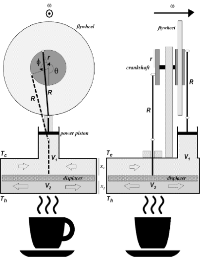
Figure 1: Schematic picture of LTD Stirling engine from two perpendicular points of view. $V_{1}$ and $V_{2}$ are the cold and the hot volumes respectively, $x_{1}+x_{2}=2r$. Open arrows indicate the movements of the gas. The flywheel moves counterclockwise and (in the instant photo) both power piston and displacer are descending. Several experimental models, whether homemade or commercial, found in the Internet fit in this scheme.

II Simple model of a Stirling engine

In this section we present a simple model of LTD Stirling engine that corresponds to a Gamma configuration. Figure 1 provides a useful insight from head-on and side of the engine running with the power piston modifying the gas volume and the displacer, continually sweeping the gas up and down. This configuration has two cylinders joined to form a single connected space with the same pressure. The cylinder with the larger cross-section contains the displacer and the other the power piston. The piston and the displacer are joined to a shaft through rods which move in parallel planes with a relative phase of $\phi\equiv\pi/2$ between the cranks. The shaft has also a flywheel.

The engine is on the top of a cup of boiling water and the remainder of the engine is in contact with the environment at room temperature. Note that the engine also would operate on the top of a cup of cold water, but in this case the flywheel would rotate in the opposite direction. The gas pressure remains uniform during the entire operation but it changes due to the motion of the piston and the action of the heat reservoirs, represented by the cup of boiling water and the room atmosphere.

In the total gas volume two zones, separated by the displacer, can be distinguished by their temperatures. Our mathematical model assumes uniform temperatures for these zones. This assumption becomes reasonable when the characteristic times associated with the movement of the pistons are much larger than those associated with the mean free path of the gas molecules. The hot zone is below the displacer where the gas is in contact with the hot reservoir at the external temperature $T_{h}$, and the cold zone is above the displacer where the gas is in contact with the cold reservoir at the external temperature $T_{c}$. However both zones have the same pressure $P$ because they are connected through the loose fit of the displacer with its cylinder. When the displacer is in its lowest position all the gas is in the cold zone, but in the rest of the cycle, the gas is never completely in either the hot or cold zone of the engine. The piston is also subjected to the atmospheric pressure $P_{0}$ from the outside.

In order to start the engine we must set in motion the flywheel externally and immediately let it move by the action of the engine. Then the mechanism of energy transfer between the hot and cold zones begins to operate and it can be qualitatively understood as follows. When the gas is swept by the displacer to the hot zone it expands, the gas pressure increases and the piston pushes up. When the gas is swept by the displacer to the cold zone it contracts, and the momentum of the machine, usually enhanced by the flywheel, pushes the piston down to compress the gas. The phase difference between displacer and piston is a crucial parameter for the efficiency and power delivered by the engine. The optimum phase is around $\phi=\pi/2$, as it has been shown.Senft3 ; Romanelli1

The piston and the displacer are connected to the shaft by rods of length $R$ as shown in Fig. 1. The piston and displacer cylinders have cross-section areas $a$ and $A$ respectively, and the crank has a rotating radius $r$. The relation between the cold and hot gas volumes, $V_{1}$ and $V_{2}$, and the flywheel angle $\theta$ can be obtained from the geometric analysis of Fig. 1, i.e.

$${V_{2}}=\left\{1+z\left[1-\cos(\theta+\phi)\right]-\sqrt{1-z^{2}\sin^{2}(\theta+\phi)}\right\}RA,$$ (1)

$${V_{1}}=2rA-{V_{2}}+{V_{p}},$$ (2)

where $z={r}/{R}$ and $V_{p}$ is the volume swept by the piston run:

$${V_{p}}=\left\{1+z\left(1-\cos\theta\right)-\sqrt{1-z^{2}\sin^{2}\theta}\right\}Ra.$$ (3)

The total volume of gas $V$ is given by

$$V={V_{1}}+{V_{2}}=2rA+{V_{p}}.$$ (4)

III Thermodynamics of an LTD Stirling engine

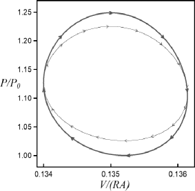
Figure 2: Dimensionless pressure-volume diagram for the initial conditions $\theta_{0}=1.46~{}\pi$ (red thick curve). The thin black curve, corresponding to the initial condition $\theta_{0}=0.46~{}\pi$, has been moved in the diagram to the current position for the sake of comparison. The arrows indicate the evolution with growing $\theta$, and the parameters are: $\phi=0.5~{}\pi$, $\alpha=1.25$, $\beta=1.23$, $a/A=0.016$ and $z=0.067$.

In previous work we have obtained an analytical generic solution for the pressure and temperatures inside of any Stirling engine.Romanelli1 That follows from the application of the first law of thermodynamics to an ideal gas subjected to polytropic processes. We have used the mentioned solution to study a particular type of Stirling engine known as Fluidyne.Romanelli2 Here we use the expression of the gas pressure as a function of the volumes (Eq. (20) of Ref. Romanelli1, ), i.e.

$$P=P_{0}\left(\frac{\alpha\,V_{10}+V_{20}}{\alpha\,V_{1}+V_{2}}\right)\left(\frac{V_{0}}{V}\right)^{\beta-1},$$ (5)

where $\alpha$ is the ratio of reservoir temperatures:

$$\alpha\equiv{T_{h}}/{T_{c}},$$ (6)

$V_{10}$, $V_{20}$ and $V_{0}$ are the initial values of $V_{1}$, $V_{2}$ and $V$ respectively (Eqs. (1), (2) and (4)), and $\beta$ is a parameter called polytropic index.romanelli The typical values of $\beta$ are such that $1\leq\beta\leq\gamma$ with $\gamma=c_{p}/c_{v}$ the quotient of the specific heats of the gas at constant pressure $c_{p}$ and constant volume $c_{v}$. For the isothermal and adiabatic cases, $\beta=1$ and $\beta=\gamma$ respectively, Eq. (5) reduces to the well known solutions found in the specialized literature of Stirling engines.Schmidt ; Bercho ; Formosa

Equation  (5) depends on $\alpha$ and it has a finite asymptotic limit when $\alpha\rightarrow\infty$. This means that after a certain value of $\alpha$, no matter how much we increase the temperature ratio the pressure and the absorbed heat are bounded, and this in turn explains why the useful work and the efficiency in any Stirling engine are asymptotically boundedRomanelli1 .

The pressure-volume diagram of the LTD Stirling engine is obtained starting from Eqs. (3), (4) and (5) and implementing numerical calculation. Such diagrams are shown in Fig. 2 for two characteristic initial values of $\theta$ which, as we shall see, correspond to the maximum and minimum engine work. The area enclosed by the curves represents the total work $W$ of the cycle, whose expression is

$$W=\oint P\,dV=\int_{\theta_{0}}^{\theta_{0}+2\pi}P{\frac{dV}{d\theta}}\,d\theta=\int_{0}^{2\pi}P{\frac{dV}{d\theta}}\,d\theta,$$ (7)

where $\theta_{0}$ is the initial angular position that determines the initial conditions for the cold and hot gas volumes. The last equality in Eq. (7) is obtained with a change of variable that contemplates the fact that the integrand is a periodic function of $\theta$. $W$ is the work available for overcoming mechanical friction losses and for providing useful power to the engine shaft. $W$ depends on $\theta_{0}$ because $P$ depends on $\theta_{0}$ through $V_{10}$, $V_{20}$ and $V_{0}$ (see Eq. (5)). Here we point out that this dependence, as far as we know, has not been explored experimentally and it would be interesting to do so.

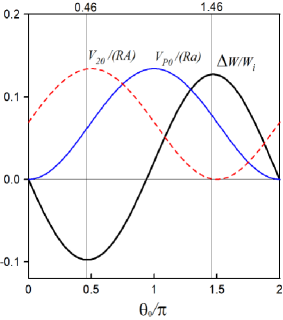
Figure 3: Relative work per cycle as a function of the initial angular condition $\theta_{0}$, in black thick line, $\Delta W=W-W_{i}$ where $W_{i}$ is the work associated with $\theta_{0}=0$. The dimensionless initial gas volume of the piston cylinder is shown with the blue thin line. The dimensionless initial gas volume of the hot zone, is shown with the red dashed line. The values of the parameters are the same as in Fig. 2.

We have integrated numerically Eq. (7) with Eqs. (5), (4) and (3) as functions of $\theta_{0}$, using the standard Simpson’s rule. Figure 3 shows that the initial volumes of cold and hot gas play a non-negligible role in the functioning of the engine. Observe that there is a difference up to $20\%$ between the maximum and minimum relative work for $\theta_{0}=1.46~{}\pi$ and $\theta_{0}=0.46~{}\pi$. It is clear that the maximum work is obtained when initially all the gas is in the cold zone, and the minimum work is obtained when initially almost all the gas is in the hot zone.

We have also integrated numerically the heat equation (Eq. (22) of Ref. Romanelli1, ) as in previous works to obtain the absorbed heat $Q_{in}$ and rejected heat $Q_{out}$, in a cycle.Romanelli1 ; Romanelli2

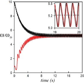
Figure 4: Dimensionless angular velocity as a function of time. Initial conditions are $\omega_{0}=10~{}\omega_{th}$ ($\omega_{th}=3\pi{b}/{I}$) for the black curve and $\omega_{0}=\omega_{th}$ for the red curve, and in both cases $\theta_{0}=1.46~{}\pi$. The inset shows a magnification of both curves when the steady states are already reached. It is seen that $\langle\omega\rangle=5.24~{}\omega_{th}$, (dashed line), and that both curves have the same asymptotic period, $\mathcal{T^{\prime}}\simeq~{}0.25$ seconds. The parameters are: $\phi=0.5~{}\pi$, $\alpha=1.25$, $\beta=1.23$, $a/A=0.016$, $z=0.067$, $b/I=0.5~{}s^{-1}$ and $I=1.2~{}{10}^{-4}kg~{}m^{2}$.

IV Dynamics of LTD Stirling engine

In order to simplify the mechanical model we neglect the masses of piston, displacer and rods. The conservation of energy imposes that all the power generated by the gas must be transferred to the the shaft, this means that

$$(P-P_{0})\frac{dV}{dt}=\tau\frac{d\theta}{dt},$$ (8)

where $\tau$ is the external torque over the shaft and, ${d\theta}/{dt}$ is the angular velocity of the flywheel. Then $\tau$ is given by

$$\tau=(P-P_{0})\frac{dV}{d\theta}.$$ (9)

The inevitable mechanical friction of the system, as well as a possible additional load incorporated to extract energy from it, generate an additional friction torque on the shaft, modeled as $-b~{}{d\theta}/{dt}$, where the sign indicates loss of power and $b$ is the damping coefficient.

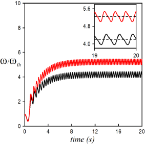
Figure 5: Dimensionless angular velocity as a function of time. Initial conditions are $\theta_{0}=0.46~{}\pi$ for the black curve, $\theta_{0}=1.46~{}\pi$ for the red curve and for both curves, $\omega_{0}=\omega_{th}$. The inset shows a magnification of both curves when the steady states are already reached. It is seen that for the black curve $\langle\omega\rangle=4.20~{}\omega_{th}$ (dashed line) and the asymptotic period is $\mathcal{T^{\prime}}\simeq~{}0.33$ s. Similarly for the red curve $\langle\omega\rangle=5.24~{}\omega_{th}$ and $\mathcal{T^{\prime}}\simeq~{}0.25$ s. The values of the parameters are the same as in Fig. 4.

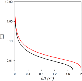
Figure 6: Dimensionless gas power (in a logarithmic scale) as a function of a generalized friction coefficient. For the upper red curve $\theta_{0}=1.46~{}\pi$, and for the lower black curve $\theta_{0}=0.46~{}\pi$, and for both curves $\omega_{0}=40~{}\omega_{th}$.

Therefore the rotational equation of motion indicates that the net external torque on the shaft determines the rate of change of its angular momentum, i.e.

$$I\frac{d^{2}\theta}{dt^{2}}=-b\frac{d\theta}{dt}+(P-P_{0})\frac{dV}{d\theta},$$ (10)

where $I$ is the flywheel moment of inertia. In order to solve Eq. (10) we need $P$ and $V$ as functions of $\theta$ given by Eqs. (4) and (5); as a result we get a nonlinear equation of $\theta$.

Multiplying Eq. (10) by the angular velocity $\omega\equiv{d\theta}/{dt}$ and integrating the resulting equation from $t=0$ to the arbitrary time $t$ we obtain the energy equation:

$$\frac{1}{2}I\omega^{2}-\frac{1}{2}I{\omega_{0}}^{2}=-b\int_{0}^{t}{\omega}^{2}\,dt^{{}^{\prime}}+\int_{\theta_{0}}^{\theta}(P-P_{0}){\frac{dV}{d\theta^{{}^{\prime}}}}\,d\theta^{{}^{\prime}},$$ (11)

where $\omega_{0}$ is the initial angular velocity. The first term on the right-hand side is the dissipative work and the second is associated with the engine power. From Eq. (5) together with Eqs. (1) and (2) it is seen that $P$ is a periodic function of $\theta$, then the second term of the right-hand side satisfies

$$\int_{\theta_{0}}^{\theta}(P-P_{0}){\frac{dV}{d\theta}}\,d\theta=n\int_{0}^{2\pi}P{\frac{dV}{d\theta}}\,d\theta+\int_{\theta_{0}}^{\theta_{r}}(P-P_{0}){\frac{dV}{d\theta}}\,d\theta,$$ (12)

where $n=(\theta-\theta_{0})[mod~{}2\pi]$ is the number of complete cycles and $\theta_{r}=(\theta-\theta_{0})-2\pi n$.

Equations (11) and (12) predict that if $b=0$ the kinetic energy grows with the number of turns $n$, however in real situations we always have $b\neq 0$. As it will be shown later our model predicts that $\omega$ has a finite asymptotic average value, with a little oscillation $\Delta\omega$ around it.

Dividing both sides of Eq. (11) by $t$ and taking the limit for $t\rightarrow\infty$ we obtain the relation between the dissipated power by the friction and power delivered by the gas

$$b\langle\omega^{2}\rangle=\frac{1}{\mathcal{T}}\int_{0}^{2\pi}P{\frac{dV}{d\theta}}\,d\theta,$$ (13)

where the flywheel period $\mathcal{T}$ is defined as

$$\mathcal{T}\equiv \lim{}\frac{t}{n}$$ (14)

$$t\rightarrow\infty\,$$ (15)

and the mean quadratic angular velocity is defined as

$$\langle\omega^{2}\rangle\equiv \lim{}{\frac{1}{t}}{\int_{0}^{t}{\omega}^{2}\,dt}.$$ (16)

$$t\rightarrow\infty\,$$ (17)

Finally, using Eq. (13) we can approximate the asymptotic average value of $\omega$, $\langle\omega\rangle\equiv{2\pi}/{\mathcal{T}}$, as

$$\langle\omega\rangle\simeq\frac{1}{2\pi b}\int_{0}^{2\pi}P{\frac{dV}{d\theta}}\,d\theta,$$ (18)

if $|\Delta\omega/\langle\omega\rangle|\ll 1$.

As mentioned, it is necessary to start the engine with an initial angular velocity $\omega_{0}$ to overcome the initial static friction and the dynamic friction that follows it. This velocity must exceed a certain threshold value $\omega_{th}$ that depends on the nonlinear dynamics of Eq. (10) which in turn depends on the parameters $I$, $b$, $\alpha$, $\beta$, $z$, $a/A$ and $\theta_{0}$. Considering the order of magnitude of the parameters used in this paper, we estimate a practical value of $\omega_{th}$ solving Eq. (10) with $P-P_{0}=0$. In this case, the solution of Eq. (10) is

$$\theta=\omega_{0}\frac{I}{b}(1-e^{-\frac{b}{I}t}).$$ (19)

We choose arbitrarily $\theta=3\pi$ in order that the flywheel can asymptotically complete at least one and half cycles. This leads to

$$\omega_{th}\sim\omega_{0}=3\pi\frac{b}{I}\ll\langle\omega\rangle.$$ (20)

Now we study numerically the dynamics of the shaft, and in particular its dependence on both the engine parameters and the initial conditions. Using a standard Runge-Kutta method for the approximate solutions of ordinary differential equations, we solved Eq. (10) with the constraints Eqs. (4) and (5).

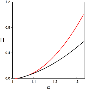
Figure 7: Dimensionless gas power as a function of the temperature ratio of heat reservoirs $\alpha$. For $\alpha=T_{h}/T_{c}\sim 1.34$ the thermal difference $T_{h}-T_{c}\sim 100~{}^{0}C$. For the upper red curve $\theta_{0}=1.46~{}\pi$, and for the lower black curve $\theta_{0}=0.46~{}\pi$, and for both curves $\omega_{0}=40~{}\omega_{th}$.

Figures 4 and  5 show the flywheel angular velocity as a function of time for two different initial conditions. Both figures show that the steady state is reached for a sufficiently large time. These asymptotic states are characterized by a constant average value with a fast small oscillation around it. Therefore our toy model predicts an asymptotic time dependent angular velocity with a well defined period $\mathcal{T^{\prime}}$, which, in principle, could be different from $\mathcal{T}$, the flywheel period.

In the case of Fig. 4 we use the same value of $\theta_{0}$ but with two different initial angular velocities $\omega_{0}$. This figure shows that in the steady state the angular velocity does not keep any correlation with its initial value; such a behavior is characteristic of dissipative systems. In the inset we see that the period $\mathcal{T^{\prime}}$ is the same for both curves, that is independent of $\omega_{0}$.

In Fig. 5 we keep the same value for $\omega_{0}$ but with two different values for $\theta_{0}$. Now the asymptotic average angular velocities have different values, this means that they depend on $\theta_{0}$, and the same is true for the periods $\mathcal{T^{\prime}}$.

At this point we emphasize that the numerical calculation shows that the flywheel period $\mathcal{T}={2\pi}/{\langle\omega\rangle}$ and the asymptotic period $\mathcal{T^{\prime}}$ of $\omega(t)$ coincide numerically, that is

$$\mathcal{T}=\mathcal{T^{\prime}}.$$ (21)

This coincidence has no obvious theoretical explanation, all the more so since the dynamical differential equation is nonlinear. In order to show that the relation given by Eq. (21) could be different, we reason as follows: When the system reaches the steady state, Figs. 4 and 5 suggest that $\omega(t)$ can be approximated by

$$\omega(t)=\langle\omega\rangle+\zeta\cos{\frac{2\pi}{\mathcal{T^{\prime}}}t},$$ (22)

where $\zeta$ is a small amplitude. However, since the flywheel angular position $\theta(t)$ is characterized by the period $\mathcal{T}$, the angular velocity (that satisfies $\omega(t)\equiv d\theta/dt$) must have also the same period. Therefore, $\mathcal{T}$ and $\mathcal{T^{\prime}}$ must satisfy the relation

$$\mathcal{T}=m\mathcal{T^{\prime}},$$ (23)

where $m$ is an integer. Our numerical calculation indicates that $m=1$ but we have no additional theoretical argument for this value.

Returning to our central development, let us define the power of the engine $\Pi$ by the right-hand side of Eq. (13), i.e.

$$\Pi\equiv\frac{1}{\mathcal{T}}\int_{0}^{2\pi}P{\frac{dV}{d\theta}}\,d\theta,$$ (24)

of course it is also true that $\Pi=b\langle\omega^{2}\rangle$.

In Fig. 6 we show $\Pi$ as a function of $b/I$ for the initial angular conditions associated with the maximum and minimum work. The upper limit of friction (i.e. the maximum value of $b/I$) is determined by the vanishing of the angular velocity, hence the vanishing of $\Pi$. The minimum value of $b/I$ has been chosen to ensure an adequate numerical convergence because asymptotically $\omega\rightarrow\infty$, the period $\mathcal{T}\rightarrow 0$ and $\Pi\rightarrow\infty$. The figure also shows that the power for $\theta_{0}=1.46~{}\pi$ is larger than for $\theta_{0}=0.46~{}\pi$, independently of $b/I$, as it is the case for the work.

Figure 7 shows the growth of $\Pi$ with the the temperature ratio $\alpha$ of the heat reservoirs. It also shows the dependence of $\Pi$ on the initial condition $\theta_{0}$.

V Conclusions

This paper developed the dynamics and thermodynamics for a Stirling engine that operates at low temperature difference. The working gas pressure is expressed analytically using an alternative thermodynamic model developed in a previous paper. This pressure depends on the hot and cold gas volumes as well as their initial conditions and the temperature ratio of the heat reservoirs.

The rotational dynamical equation for the shaft includes terms related to the energy delivered by the engine and to the energy dissipated by friction. This nonlinear equation, which we solved numerically, has an explicit dependence on the initial gas volumes through the initial angular position $\theta_{0}$.

We showed numerically that both the maximum shaft work and power are obtained when at the start all the gas is in the cold zone. Conversely the minimum shaft work and power are obtained when initially almost all the gas is in the hot zone. These results are independent of: (a) the shaft initial angular velocity, (b) the shaft friction intensity, (c) the temperature ratio of the heat reservoirs.

In order to choose initial conditions we estimated a minimal initial flywheel speed to start the engine. Our model predicts that the flywheel velocity achieves a finite asymptotic average value with a small periodic oscillation around it. Our system has a dissipative dynamics, however its steady state showed an unexpected dependence on the initial angular position. This means that the angular velocity evolves to an attractor independently of its initial value but dependent on the initial angular position. This asymmetric behavior is due the fact that the model incorporated the initial angular position in the dynamical equation but not the initial angular velocity.

Summarizing, this paper describes the operation of the LTD Stirling engine in a simple and understandable way, highlighting some unknown aspects of its behavior.

References

- (1) D. García Menéndez, “Desarrollo de motores de Stirling para aplicaciones solares,” PhD thesis, (Universidad de Oviedo, 2013).
- (2) Caleb C. Lloyd, “A low temperature differential Stirling engine for power generation,” Master of Engineering thesis, (University of Canterbury, 2009).
- (3) J.S. Reid, “Stirling Stuff”(2016), https://arxiv.org/abs/1604.02362.
- (4) R. Sier, Hot Air Caloric and Stirling Engines: A History, (L. A. Mair, Chelmsford, U.K., 1999), Vol. 1.
- (5) G. Walker, J.R. Senft, Free Piston Stirling Engines, (Springer-Verlag, Berlin, 1980).
- (6) R. Darlington, K. Strong, Stirling and Hot Air Engines, (The Crowood Press, Marlborough, 2005).
- (7) J.R. Senft, “Optimum Stirling engines geometry,” Int. J. Energy Res. 26, 1087-1101 (2002).
- (8) Kolin Ivo, “Stirling Motor - History, Theory, Practice,” (Zagreb University Publications, Dubrovnik, 1991).
- (9) Kolin Ivo, Koscak-Kolin, Sonja and Golub, Miroslav, “Geothermal Electricity Production by Means of the Low Temperature Difference Stirling Engine,” (Kyushu: Faculty of Mining, Geology and Petroleum Engineering, World Geothermal Congress, 2000)
- (10) J.R. Senft, An Introduction to Low Temperature Differential Stirling Engines, (Moriya Press., 1996).
- (11) J.R. Senft, “Theoretical limits on the performance of Stirling engines,” Int. J. Energy Res. 22, 991-1000 (1998).
- (12) B. Kongtragool, S. Wongwises, “Thermodynamic analysis of a Stirling engine including dead volumes of hot space, cold space and regenerator,” Renewable Energy, 31, 345-359 (2006).
- (13) G. Barreto, P. Canhoto, “Modelling of a Stirling engine with parabolic dish for thermal to electric conversion of solar energy,” Energy Convers. Manage. 132, 119-135 (2017).
- (14) H. Jokar, A. R. Tavakolpour-Salej, “A novel solar-powered active low temperature differential Stirling pump,” Renewable Energy, 81, 319-337 (2015).
- (15) L.G. Thieme, S. Qiu, M.A. White, “Technology development for a Stirling radioisotope power system,” NASA TM-2000-209791 (2000).
- (16) R.G. Lange, W. P. Carroll, “Review of recent advances of radioisotope power systems,” Energy Convers. Manage., 49, 393-401 (2008).
- (17) I. M. Santos Ráez, “Estudio de un motor Stirling con absorbedor interno alimentado con energía solar,” PhD thesis, (Universidad de Málaga, 2015).
- (18) G. Barreto, P. Canhoto, “Modelling of a Stirling engine with parabolic dish for thermal to electric conversion of solar energy,” Energy Convers. Manage., 132, 119-135 (2017).
- (19) M.W. Zemansky, R.H. Dittman, Heat and Thermodynamics, (McGraw-Hill, London, 1997).
- (20) A. Romanelli, “Alternative thermodynamic cycle for the Stirling machine,” Am. J. Phys. 85, 926-931 (2017).
- (21) A. Romanelli, “The Fluidyne engine,” Am. J. Phys. 87, 33-37 (2019).
- (22) A. Romanelli, I.Bove, F.González, “Air expansion in a water rocket,” Am. J. Phys. 81, 762-766 (2013).
- (23) G. Schmidt, “Theorie der Lehmann’schen kalorischen Maschine,” Z. Ver. Deut. Ing. 15, 1 (1871).
- (24) I.Urieli, D.Berchowitz, Stirling Cycle Engine Analysis, (Adam Hilger, Bristol, 1983).
- (25) F.Formosa, G.Despesse, “Analytical model for Stirling cycle machine design,” Energy Convers. Manage., 51, 1855-1863 (2010).