Application of the diffusion equation to prove scaling invariance on the transition from limited to unlimited diffusion

Abstract

The scaling invariance for chaotic orbits near a transition from unlimited to limited diffusion in a dissipative standard mapping is explained via the analytical solution of the diffusion equation. It gives the probability of observing a particle with a specific action at a given time. We show the diffusion coefficient varies slowly with the time and is responsible to suppress the unlimited diffusion. The momenta of the probability are determined and the behavior of the average squared action is obtained. The limits of small and large time recover the results known in the literature from the phenomenological approach and, as a bonus, a scaling for intermediate time is obtained as dependent on the initial action. The formalism presented is robust enough and can be applied in a variety of other systems including time dependent billiards near a transition from limited to unlimited Fermi acceleration as we show at the end of the letter and in many other systems under the presence of dissipation as well as near a transition from integrability to non integrability.

Since the observation and a phenomenological characterization Paper1 of scaling invariance in the chaotic sea near a transition from integrability to non integrability in a Fermi Ulam model Paper2 , the formalism using homogeneous and generalized function leading to a set of critical exponents Book1 has been widely used in a variety of systems to investigate dynamical properties near dynamical phase transitions including oscillating spring mass system Paper3 , billiards Paper4 ; Paper5 , scaling in social media Paper6 , in waveguides Paperadd and in many other systems. In a majority of the cases the scaling is closely connected with diffusion yielding applications in different subjects of science being therefore observed in systems from pollen diffusing Paper7 , in disease propagation Paper8 ; Paper9 ; Paper10 , in pests spreading Paper11 and many others hence making the topic of wide interest.

In this letter our aim is to characterize analytically a transition from limited to unlimited diffusion by using the diffusion equation Book2 applied in a paradigmatic model in nonlinear science the so called dissipative standard mapping Book3 and the success of the formalism allowed us to extend its applicability to time dependent billiards. The mapping is written in terms of two equations $I_{n+1}=(1-\gamma)I_{n}+\epsilon\cos(\theta_{n})$ and $\theta_{n+1}=(\theta_{n}+I_{n+1})~{}\rm{mod}(2\pi)$ where $\gamma\in[0,1]$ is the dissipative parameter and $\epsilon$ corresponds to the intensity of the nonlinearity. This system has two well known transitions Book3 for $\gamma=0$ (conservative case): (i) A transition from integrability for $\epsilon=0$ where the phase space is foliated to non integrability when $\epsilon\neq 0$ and mixed structure is presented in the phase space including periodic islands, chaotic seas and invariant spanning curves limiting the diffusion to a closed region; (ii) at a critical value of $\epsilon_{c}=0.9716\ldots$, the system admits a transition from local chaos when $\epsilon<\epsilon_{c}$ to globally chaotic dynamics for $\epsilon>\epsilon_{c}$ where invariant spanning curves are no longer present and, depending on the initial conditions, chaos can diffuse unbounded in the phase space. The determinant of the Jacobian matrix is $\det~{}J=(1-\gamma)$ and for $\gamma\neq 0$ the Liouville’s theorem is violated leading to the existence of attractors in the phase space. For large enough $\epsilon$, typically $\epsilon>10$ sinks are not observed in the phase space hence leading the dynamics to have chaotic attractors in the limit of small values of $\gamma$. At such limit one is facing a transition from limited ($\gamma\neq 0$) to unlimited ($\gamma=0$) diffusion for the variable $I$ which is the transition we consider in this letter. Our main goal in this letter is to fix up an open problem in the nonlinear community discussing the scaling invariance present in the transition from limited for $\gamma\neq 0$ to unlimited diffusion when $\gamma=0$, so far analytically for large values of $\epsilon$. As far as we can tell, this scaling investigation has only been described using a phenomenological approach Paper12 assuming a set of scaling hypotheses allied with a homogeneous function hence leading to a set of critical exponents leaving a lack on the analytical solution which to the best knowledge of the authors has never been made. At the same time, this letter fix up this gap in the literature and the present approach is proved to be valid and can be used in a wide class of other systems including transition from limited to unlimited Fermi acceleration in time dependent billiards as we shown in the end of the letter, integrability to non integrability in nonlinear mappings and many others.

The range of parameters we are interested in to validate the transition is $\gamma$ positive and small, typically $\gamma\in[10^{-5},10^{-2}]$ and $\epsilon>10$, which drives the system to high nonlinearities and absence of sinks in the phase space. At such a window of parameters a transition from limited, $\gamma\neq 0$ to unlimited, $\gamma=0$, diffusion is observed. A typical plot of the phase space is shown in Figure 1(a) illustrating a chaotic attractor for the parameter $\epsilon=10$ and $\gamma=10^{-3}$ together with the probability distribution along the chaotic attractor shown in Figure 1(b). We see from Figure 1(a) the density of points concentrate around $I\cong 0$ and is symmetric with respect to the vertical axis. The distribution fades soon as it goes apart from the origin. The positive Lyapunov exponent measured Paper13 for the chaotic attractor shown in Fig. 1(a) was $\lambda=3.9120(1)$.

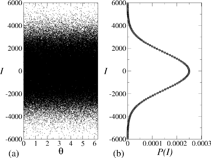
Figure 1: (a) Plot of the phase space for the standard dissipative mapping considering the parameters $\epsilon=100$ and $\gamma=10^{-3}$. (b) Normalized probability distribution for the chaotic attractor shown in (a).

Given an initial condition near $I\cong 0$ the particle diffuses along the chaotic attractor. The natural observable to characterize the diffusion is the average squared action $I_{rms}(n)=\sqrt{{{1}\over{M}}\sum_{i=1}^{M}I^{2}_{i}}$ where $M$ corresponds to an ensemble of different initial conditions along the chaotic attractor. To obtain such observable we need to solve the diffusion equation that gives the probability to observe a specific action $I$ at a given time $n$, i.e. $P(I,n)$. The diffusion equation is written as

$${{\partial P(I,n)}\over{\partial n}}=D{{\partial^{2}P(I,n)}\over{\partial I^{2}}},$$ (1)

where the diffusion coefficient $D$ is obtained from the first equation of the mapping by using $D={{\overline{I^{2}}_{n+1}-\overline{I^{2}_{n}}}\over{2}}$. A straightforward calculation assuming statistical independence between $I_{n}$ and $\theta_{n}$ at the chaotic domain leads to

$$D(\gamma,\epsilon,n)={{\gamma(\gamma-2)}\over{2}}\overline{I^{2}}_{n}+{{\epsilon^{2}}\over{4}}.$$ (2)

The expression of $\overline{I^{2}}_{n}$ is obtained also from the first equation of the mapping assuming that $\overline{I^{2}}_{n+1}-\overline{I^{2}}_{n}={{\overline{I^{2}}_{n+1}-\overline{I^{2}}_{n}}\over{(n+1)-n}}\cong{{d\overline{I^{2}}}\over{dn}}=\gamma(\gamma-2)\overline{I^{2}}+{{\epsilon^{2}}\over{2}}$, whose solution is

$$\overline{I^{2}}(n)={{\epsilon^{2}}\over{2\gamma(2-\gamma)}}+\left(I_{0}^{2}+{{\epsilon^{2}}\over{2\gamma(\gamma-2)}}\right)e^{-\gamma(2-\gamma)n}.$$ (3)

To compare with the experimental observable Eq. (3) must be averaged over the orbit, leading to

$$< \overline{I^{2}} (n)>={{1}\over{n+1}}\sum_{i=0}^{n}\overline{I^{2}}(i)={{\gamma(\gamma-2)}\over{2(n+1)}}\times$$ (4)

$$\times \left[I^{2}_{0}+{{\epsilon^{2}}\over{2\gamma(\gamma-2)}}\left({{1-e^{-(n+1)\gamma(2-\gamma)}}\over{1-e^{-\gamma(2-\gamma)}}}\right)\right].$$

To obtain an unique solution for Eq. (1) we impose the following boundary conditions $\lim_{I\rightarrow\pm\infty}P(I)=0$ with the initial condition $P(I,0)=\delta(I-I_{0})$ that warrants all particles leave from the same initial action but with $M$ different initial phases $\theta\in[0,2\pi]$. Although the diffusion coefficient $D$ depends on $n$ its variation is slow and little from the instant $n$ to $n+1$. This property allows us to consider it constant to obtain the solution of the diffusion equation. However, soon as the solution is obtained, the expression of $D$ from Eq. (2) is incorporated to the solution. The technique used to solve Eq. (1) is the Fourier transform Book4 . Because the probability is normalized, i.e. $\int_{-\infty}^{\infty}P(I,n)dI=1$, we can define a function

$$R(k,n)=\mathcal{F}\{P(I,n)\}={{1}\over{\sqrt{2\pi}}}\int_{-\infty}^{\infty}P(I,n)e^{ikI}dI.$$ (5)

Differentiating $R(k,n)$ with respect to $n$ and from the property that $\mathcal{F}\left\{{{\partial^{2}P}\over{\partial I^{2}}}\right\}=-k^{2}R(k,n)$ we end up the following equation to be solved ${{dR}\over{dn}}(k,n)=-Dk^{2}R(k,n)$, which leads to

$$R(k,n)=R(k,0)e^{-Dk^{2}n}.$$ (6)

Considering the initial condition we have that $R(k,0)=\mathcal{F}\{\delta(I-I_{0})\}={{1}\over{\sqrt{2\pi}}}e^{ikI_{0}}$. Inverting the expression of $R(k,n)$ we obtain

$$P(I,n) = {{1}\over{\sqrt{2\pi}}}\int_{-\infty}^{\infty}R(k,n)e^{-ikI}dk,$$ (7)

$$= {{1}\over{\sqrt{4\pi Dn}}}e^{-{{(I-I_{0})^{2}}\over{4Dn}}}.$$

Equation (7) satisfies both the boundary and initial condition as well as the diffusion equation (1). It is also normalized by construction. The observable we want to characterize is $\overline{I^{2}}(n)=\int_{-\infty}^{\infty}I^{2}P(I,n)dI$, which leads to $\overline{I^{2}}(n)=\sqrt{2D(n)n+I_{0}^{2}}$. Using $D(n$) obtained from Eq. (2), we end up with the expression of $I_{rms}(n)$ as

$$I_{rms}(n)=\sqrt{I_{0}^{2}+{{n\gamma(\gamma-2)}\over{n+1}}\left[I_{0}^{2}+{{\epsilon^{2}}\over{2\gamma(\gamma-2)}}\right]\left[{{-(n+1)\gamma(2-\gamma)}\over{1-e^{-\gamma(2-\gamma)}}}\right]}.$$ (8)

Let us discuss specific limits of $n$ and its consequences to Eq. (8). The first limit is $n=0$, which leads to $I_{rms}(0)=I_{0}$, in well agreement to the initial condition. The second limit is $n\rightarrow\infty$. At such a limit we have

$$I_{rms}=\sqrt{I_{0}^{2}+\gamma(\gamma-2)\left[I_{0}^{2}+{{\epsilon^{2}}\over{2\gamma(\gamma-2)}}{{1}\over{1-e^{-\gamma(2-\gamma)}}}\right]},$$ (9)

and that when expanding in Taylor series up to first order the term $1-e^{-\gamma(2-\gamma)}\cong\gamma(2-\gamma)$ we obtain

$$I_{rms}={{1}\over{\sqrt{2(2-\gamma)}}}\epsilon\gamma^{-1/2}.$$ (10)

Let us discuss this result prior move on. It is known in the literature Paper12 that the critical exponents $\alpha_{1}$ and $\alpha_{2}$ can be obtained from the scaling theory. It was supposed that for large enough $n$, the stationary state is given by $I_{rms}\propto\epsilon^{\alpha_{1}}\gamma^{\alpha_{2}}$. An immediate comparison of this scaling hypothesis with Eq. (10) leads to a remarkable results of $\alpha_{1}=1$ and $\alpha_{2}=-{{1}\over{2}}$, in very well agreement with the phenomenological prediction discussed in Ref. Paper12 . Interestingly, such a result can also be obtained from the own equations of the mapping imposing that $\overline{I^{2}}_{n+1}=\overline{I^{2}}_{n}=\overline{I^{2}}_{sat}$, yielding $I_{sat}={{1}\over{\sqrt{2(2-\gamma)}}}\epsilon\gamma^{-1/2}$.

The limit of small $n$ is the third limit we consider. Assuming that the initial action $I_{0}\cong 0$, hence negligible as compared to $\epsilon$ and doing a Taylor expansion on the exponential of the numerator from Eq. (9) we obtain $I_{rms}(n)\cong\sqrt{{{\epsilon^{2}}\over{2}}n}$. This result proves that for short $n$, an ensemble of particles diffuses along the chaotic attractor analogously as a random walk motion, hence with diffusion exponent $\beta=1/2$, i.e., normal diffusion. From Ref. Paper12 a scaling hypothesis at the limit of small $n$ is $I_{rms}(n)\propto(n\epsilon^{2})^{\beta}$, with $\beta=1/2$ in well agreement with the theoretical prediction discussed above.

A fourth interesting limit we want to take into account is again intermediate $n$ but non negligible $I_{0}$ such that $0<I_{0}<I_{sat}$. At such windows of $I_{0}$ and $n$, an additional crossover is observed when $n_{x}^{\prime}\cong 2{{I_{0}^{2}}\over{\epsilon^{2}}}$. This crossover had already been observed in Paper1 when a phenomenological approach was proposed and confirmed analytically in Paper14 .

A fifth limit is in the case of $I_{0}\cong 0$, leading to a growth in $I_{rms}$ for short $n$ followed by a crossover and a bend towards the regime of saturation. Such a characteristic crossover is given by $n_{x}\cong{{1}\over{2-\gamma}}\gamma^{-1}$. From the scaling approach as discussed in Ref. Paper12 it is assumed that $n_{x}\propto\epsilon^{z_{1}}\gamma^{z_{2}}$ and that $z_{1}=0$ and $z_{2}=-1$, as obtained above.

The last regime of interest is considered when $I_{0}\gg{{\epsilon^{2}}\over{2\gamma(2-\gamma)}}$. At this limit, Equation (8) is rewritten as

$$I_{rms}(n)=\sqrt{I_{0}^{2}e^{-(n+1)\gamma(2-\gamma)}+\epsilon^{2}{{(1-e^{-(n+1)\gamma(2-\gamma)})}\over{2\gamma(2-\gamma)}}}.$$ (11)

The leading term for small $n$ is $I_{rms}(n)=I_{0}e^{-(n+1){{\gamma(2-\gamma)}\over{2}}}$ while the stationary state is obtained at the limit of $\lim_{n\rightarrow\infty}I_{rms}={{\epsilon}\over{\sqrt{2(2-\gamma)}}}\gamma^{-1/2}$ , in well agreement with the previous results.

Figure 2(a) shows

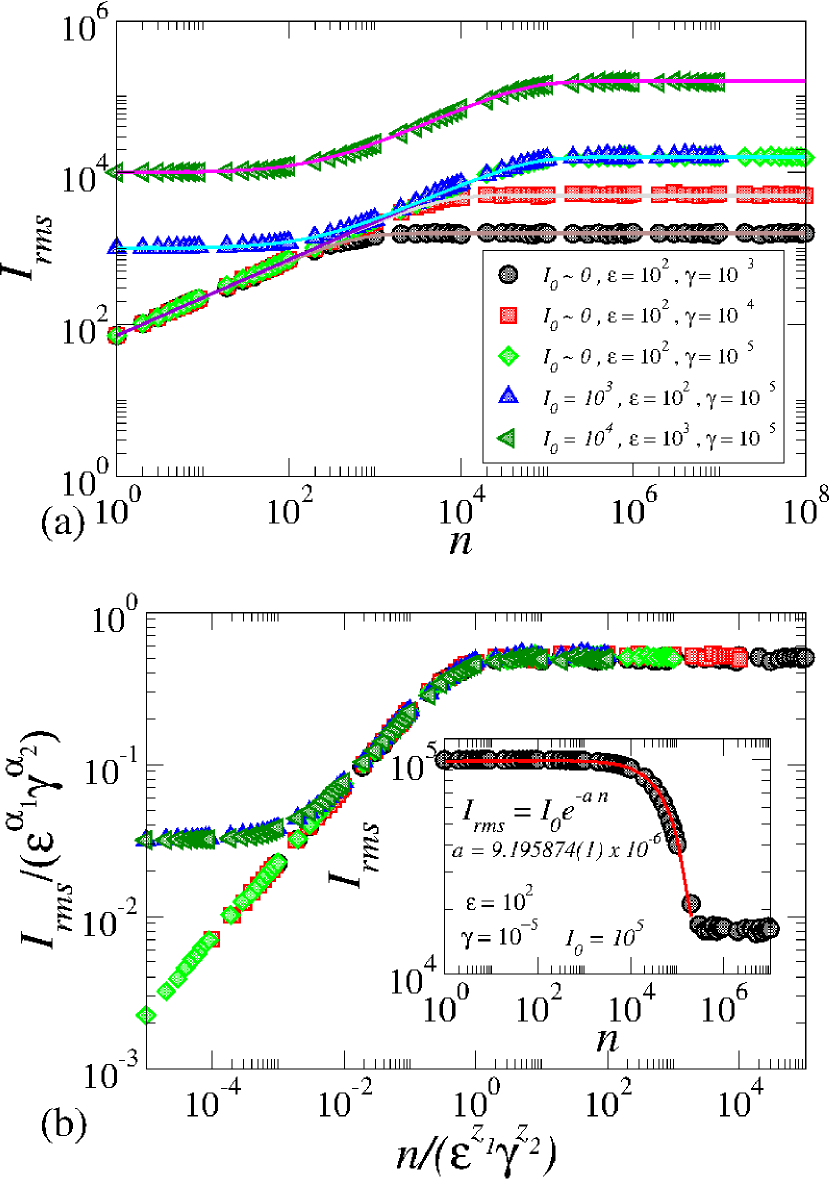
Figure 2: (a) Plot of the phase space for the standard dissipative mapping considering the parameters $\epsilon=100$ and $\gamma=10^{-3}$. (b) Normalized probability distribution for the chaotic attractor shown in (a). Inset of (b) shows an exponential decay to the attractor.

a plot of $I_{rms}~{}vs.~{}n$ for different control parameters and initial conditions, as labeled in the figure. Filled symbols correspond to the numerical simulation obtained direct from the iteration of the dynamical equations of the mapping considering an ensemble of $M=10^{3}$ different initial particles, all starting with same action $I_{0}$, as shown in Fig. 2(a) and different initial phases $\phi_{0}\in[0,2\pi]$. Analytical result from Eq. (8) is plotted as continuous line. The overlap of the curves is remarkable good. Figure 2(b) shows the overlap of the curves plotted in (a) onto a single and hence universal curve. The scaling transformations are: (i) $I_{rms}\rightarrow I_{rms}/(\epsilon^{\alpha_{1}}\gamma^{\alpha_{2}})$; (ii) $n\rightarrow n/(\epsilon^{z_{1}}\gamma^{z_{2}})$. The inset of Fig. 2(b) shows the exponential decay as predicted by Eq. (11). The control parameters used in the inset were $\epsilon=10^{2}$ and $\gamma=10^{-5}$ and with the initial action $I_{0}=10^{5}$. The slope of the exponential decay obtained numerically is $a=9.195874(1)\times 10^{-6}$, which is close to $\gamma(2-\gamma)/2\cong 9.99995\times 10^{-6}$.

Let us now show applicability of the formalism developed to a far more complicate system, indeed a time dependent billiard Paper15 . The boundary confining an ensemble of non interacting particle is written as $R(\theta,\eta,t)=1+\eta f(t)\cos(p\theta)$ with $p$ integer. The case of $\eta=0$ corresponds to the circle billiard, which is integrable and that has foliated phase space Book5 . For $\eta\neq 0$ and $f(t)=const.$ the phase space is of mixed kind exhibiting chaos, invariant spanning curves and periodic islands Paper16 . Fermi acceleration Paper2 is observed when $f(t)=1+\epsilon\cos(\omega t)$, where scaling properties Paper18 are also observed. We shall consider that $f(t)=1+\epsilon\cos(\omega t+Z)$ where $Z\in[0,2\pi]$ is a random number generated at each collision of the particle with the moving boundary. The dynamics of each particle is given in terms of a $4-D$ nonlinear mapping for the variable velocity of the particle $V_{n}$, instant of the collision $t_{n}$, polar angle $\theta_{n}$ and angle that the trajectory of the particle makes $\alpha_{n}$ with a tangent line at the instant of the collision. The velocity of the boundary at the instant of the impact is $\vec{V}_{b}(t)={{d\vec{R}_{b}}\over{dt}}(t+Z)$. The reflection laws are given by $\vec{V}^{\prime}_{n+1}\cdot\vec{T}_{n+1}=\vec{V}^{\prime}_{n}\cdot\vec{T}_{n+1}$ and $\vec{V}^{\prime}_{n+1}\cdot\vec{N}_{n+1}=-\gamma\vec{V}^{\prime}_{n}\cdot\vec{N}_{n+1}$ where $\gamma\in[0,1]$ corresponding to a restitution coefficient. The case of $\gamma=1$ leads to a non dissipative case while $0<\gamma<1$ corresponds to the dissipative case. $\vec{T}$ and $\vec{N}$ are the tangent and normal unit vectors at the instant of the impact and ^′ is to consider the momentum conservation law at the moving referential frame. The case $\gamma=1$ leads to unlimited diffusion for the velocity of the particles, hence producing Fermi acceleration while $\gamma<1$ suppress such a diffusion generating a set of points in the phase far from the infinity. The diffusion coefficient obtained for this model is

$$D(\eta,\epsilon,\gamma,n)={{\overline{V^{2}}_{n}}\over{4}}+{{(1+\gamma)^{2}\eta^{2}\epsilon^{2}}\over{16}},$$ (12)

where the expression for $\overline{V^{2}}_{n}$ is

$$\overline{V^{2}}(n)=V_{0}^{2}e^{-n{{(\gamma^{2}-1)}\over{2}}}+{{(1+\gamma)\eta^{2}\epsilon^{2}}\over{4(1-\gamma)}}\left(1-e^{-{{n(\gamma^{2}-1)}\over{2}}}\right).$$ (13)

As discussed in Ref. Paper19 , the behavior of the $V_{rms}(n)$ can be summarized as: (i) for short $n$, $V_{rms}(n)\propto n^{\beta}$; (ii) for large enough $n$, it is observed that $V_{sat}\propto(1-\gamma)^{\alpha_{1}}(\eta\epsilon)^{\alpha_{2}}$, (iii) finally the crossover iteration number is written as $n_{x}\propto(1-\gamma)^{z_{1}}(\eta\epsilon)^{z_{2}}$. Doing the same procedure we made along on the paper we end up with the following set of critical exponents $\alpha_{1}=-0.5$, $z_{1}=-1$, $\alpha_{2}=1$, $z_{2}=0$ and $\beta=0.5$ as earlier obtained in Ref. Paper19 by using the thermodynamical approach.

As a summary, the diffusion equation is used with a great success to describe a transition from limited to unlimited diffusion leading to an analytical explanation of the scaling invariance present in such a transition. A set of critical exponents, so far obtained from numerical and phenomenological way were obtained analytically corroborating for a robust and general interest of the procedure.

EDL thanks support from CNPq (301318/2019-0) and FAPESP (2019/14038-6), Brazilian agencies. CMK thanks to CAPES for support.

References

- (1) E. D. Leonel, J. K. L. Silva, P. V. E. McClintock, Phys. Rev. Lett 93, 014101 (2004).
- (2) E. Fermi, Phys. Rev. 75, 1169 (1949).
- (3) F. Reif, Fundamentals of statistical and thermal physics, New York: McGraw-Hill (1965).
- (4) O. F. de Alcantara Bonfim, Phys. Rev. E 79, 056212 (2009).
- (5) D. F. M. Oliveira, M. Robnik, International Journal of Bifurcation and Chaos 22, 1250207 (2012).
- (6) E. D. Leonel, L. A. Bunimovich, Phys. Rev. E 82, 016202 (2010).
- (7) D. F. M. Oliveira, K. S. Chan, E. D. Leonel, Physics Letters A 382, 47 (2018).
- (8) E. D. Leonel, Phys. Rev. Lett 98, 114102 (2007).
- (9) W. F. Morris, Ecology 74, 493 (1993).
- (10) S. A. El-Kafrawy et al, The Lancet Planetary Health 3, e521 (2019).
- (11) Z. Xu, Y. Zhang, IMA J. of Applied Mathematics 80, 1124 (2015).
- (12) Y. Lou, X. Q. Zhao, J. Math. Biol. 62, 543 (2011).
- (13) W. S. Jo, H. Y. Kim, B. J. Kim, J. Korean Phys. Soc. 70, 108 (2017).
- (14) V. Balakrishnan, Elements of nonequilibrium statistical mechanics, Ane Books India, New Delhi (2008).
- (15) A. J. Lichtenberg, M. A. Lieberman, Regular and chaotic dynamics (Appl. Math. Sci.) 38, Springer Verlag, New York (1992).
- (16) D. F. M. Oliveira, M. Robnik, E. D. Leonel, Phys. Lett. A 376, 723 (2012).
- (17) J.-P. Eckmann and D. Ruelle, Rev. Mod. Phys. 57, 617, (1985).
- (18) E. Butkov, Mathematical Physics, Addison-Wesley Pub. Co., (1968)
- (19) M. S. Palmero, G. I. Díaz, P. V. E. McClintock, E. D. Leonel, Chaos 30, 013108 (2020).
- (20) A. Y. Loskutov, A. B. Ryabov, and L. G. Akinshin, J. Exp. Theor. Phys. 89, 966 (1999).
- (21) N. Chernov, R. Markarian, Chaotic Billiards (American Mathematical Society, Vol. 127, 2006)
- (22) M. V. Berry, Eur. J. Phys. 2, 91, (1981).
- (23) E. D. Leonel, D. F. M. Oliveira, A. Loskutov, Chaos 19, 033142 (2009).
- (24) E. D. Leonel, M. V. C. Gália, L. A. Barreiro, D. F. M. Oliveira, Phys. Rev. E 94, 062211 (2016).