Transport and tumbling of polymers in viscoelastic shear flow

Abstract

Polymers in shear flow are ubiquitous and we study their motion in a viscoelastic fluid under shear. Employing dumbbells as representative, we find that the center of mass motion follows: $\langle x^{2}_{c}(t)\rangle\sim\dot{\gamma}^{2}t^{\alpha+2},~{}0<\alpha<1$, generalizing the earlier result: $\langle x^{2}_{c}(t)\rangle\sim\dot{\gamma}^{2}t^{3}~{}(\alpha=1)$. Motion of the relative coordinate, on the other hand, is quite intriguing in that $\langle x^{2}_{r}(t)\rangle\sim t^{\beta}$ with $\beta=2(1-\alpha)$ for small $\alpha$. This implies nonexistence of the steady state. We remedy this pathology by introducing a nonlinear spring with FENE-LJ interaction and study tumbling dynamics of the dumbbell. The overall effect of viscoelasticity is to slow down the dynamics in the experimentally observed ranges of the Weissenberg number. We numerically obtain the characteristic time of tumbling and show that small changes in $\alpha$ result in large changes in tumbling times.

Introduction: Viscoelastic fluids under shear are ubiquitous, especially in biological systems, and aid in transport of biomolecules in-vivo. Viscoelasticity, as the name suggests, is the property of a material comprising of both viscous and elastic behavior maxwell . Almost all materials with biological or engineering interests are viscoelastic to some degree lakes . The elastic component of the material tends to bring it back to its original configuration when put under stress jones . As a result, motion in viscoelastic media is generally slower, i.e.- the mean square displacement $\langle x^{2}(t)\rangle\sim t^{\alpha}$ jeon , with $0<\alpha<1$, consequent of the anti-persistent correlations in successive displacements mandelbrot . Viscoelastic subdiffusion frequently arises in motion in biological domains, e.g.- motion in crowded fluids Mweiss , cytoplasm of living cells weber , locus of a chromosome in eukaryotes israel , etc.

Even though a useful representative of system dynamics, a single particle description is not fully appropriate when it comes to investigating systems with internal degrees of freedom, e.g.- polymers. In addition, polymers constitute the basic building blocks of the macromolecules like DNA and proteins. Hence, it becomes natural to investigate the dynamical aspects of a polymer in viscoelastic media. However, most of the polymer transport in-vivo takes place in viscoelastic fluids under shear, wherein they not only move but also tumble along, i.e.- an end-to-end rotation. The phenomena of polymer tumbling is well understood for the case of viscous shear flows smith ; leduc . And arises when the relaxation time of the polymer is larger than the time-scale of flow deformation usabiaga , with characteristic tumbling time varying sublinearly with the flow rate schroeder ; winkler . However, a majority of studies involving tumbling do not cover the practically important case of shear flows arising in viscoelastic media, e.g.- polymer plastics and most of the biological materials ozkaya .

These observations raise an interesting question: what are the dynamical characteristics of a polymer in a viscoelastic fluid under shear? This is a question of immense practical significance, which we answer in the present work employing a dumbbell which is the simplest form of a polymer. For the two masses connected by a harmonic spring, we show both analytically and numerically that the separation grows without bounds. This implies towards the nonexistence of steady state and essentially means that tumbling cannot be addressed using a linear system. We remedy this pathology by introducing a finitely extensible nonlinear elastic spring with repulsive part of the Lennard-Jones interaction (FENE-LJ) herrchen ; grest . Thus, allowing us to address tumbling.

Generalized Langevin equation in shear flows: The generalized Langevin equation (GLE) zwanzig describing the motion of a dumbbell in a viscoelastic material under shear reads:

$$\int^{t}_{0}dt^{\prime}\eta(t-t^{\prime})(\dot{\bf r}_{i}-\dot{\gamma}y_{i}{\bf i})(t^{\prime}) =-\nabla_{i}V(|{\bf r}_{i}-{\bf r}_{j}|)+{\bf\xi}_{i}(t),$$ (1)

where ${\bf r}_{i}\equiv(x_{i},y_{i},z_{i})$, with $i=1,2$ and $i\neq j$ denote the two particles. The shear rate $\dot{\gamma}$ defines the Weissenberg number Wi $=\tau_{0}\dot{\gamma}$, in terms of the relaxation time $\tau_{0}$ of the dumbbell in the absence of any flow. The noise vectors ${\bf\xi}_{1}$ and ${\bf\xi}_{2}$ are Gaussian random variables with correlation matrices: $\langle{\bf\xi}_{i}(t){\bf\xi}^{T}_{j}(t^{\prime})\rangle=\delta_{ij}k_{B}T\eta(|t-t^{\prime}|){\bf I}_{3}$, consistent with the fluctuation dissipation relation kubo , where ${\bf I}_{3}$ denotes the $3\times 3$ identity matrix. For the case of harmonically interacting dumbbells we choose $V(|{\bf r}_{i}-{\bf r}_{j}|)=\frac{1}{2}\omega^{2}_{0}({\bf r}_{i}-{\bf r}_{j})^{2}$, which is a Rouse polymer of size $N=2$ rouse .

The term inside the integral in Eq. (1) is the memory kernel representing a time-dependent friction. Consequently, the present state depends on the entire history. Physically, the GLE renders itself derivable in terms of mechanical equations for a particle interacting with a thermal bath, in terms of the spectral density of the bath oscillators weiss ; raz . To address the problem at hand, we employ a power law decaying form for the memory kernel: $\eta(t)=\eta_{\alpha}t^{-\alpha}/\Gamma(1-\alpha)$, with $0<\alpha<1$ gemant . With this form of memory kernel, the GLE results in a subdiffusion for the motion of a free particle goychuk ; wang .

Center of mass motion for linear spring: Absence of any external force on the dumbbell allows us to separate its dynamics into the motion of center of mass and motion about the center of mass. The coordinate of the center of mass ${\bf r}_{c}=\frac{{\bf r}_{1}+{\bf r}_{2}}{2}$ evolves as:

$$\int^{t}_{0}dt^{\prime}\eta(t-t^{\prime})(\dot{\bf r}_{c}-\dot{\gamma}y_{c}{\bf i})(t^{\prime})={\bf\xi}_{c}(t),$$ (2)

where $\xi_{c}(t)=[\xi_{1}(t)+\xi_{2}(t)]/2$ is Gaussian noise with mean zero and correlation: $\langle\xi_{c}(t)\xi^{T}_{c}(t^{\prime})\rangle=\frac{1}{2}k_{B}T\eta(|t-t^{\prime}|){\bf I}_{3}$.

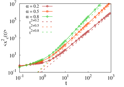
Figure 1: Mean square displacement of the center of mass motion $x_{c}$ along the shear flow direction for varying $\alpha$, with respective line fits. Parameter values for numerical calculation are: $\dot{\gamma}=1,~{}\eta_{\alpha}=1$ and $k_{B}T/2=1$.

It is evident looking at Eq. (2) that the center of mass moves like a free particle in shear flow. Interestingly, the $y$ (and $z$) components of motion do not feel the effect of shear flow, with the well known two-point correlation: $\langle y(t_{1})y(t_{2})\rangle=k_{B}T/2\eta_{\alpha}[t_{1}^{\alpha}+t_{2}^{\alpha}-|t_{1}-t_{2}|^{\alpha}$] jeon . The $x$ component of motion is, however, affected by the presence of shear flow which is directed along the $x$-axis. Invoking the Laplace transform of Eq. (2) allows us to decouple the convolution of the memory kernel $\eta$ and local velocity. As a result, the time evolution of the $x$-coordinate of the center of mass evolves as:

$$x_{c}(t)=\dot{\gamma}\int^{t}_{0}dt^{\prime}y_{c}(t^{\prime})+\int^{t}_{0}dt^{\prime}g(t-t^{\prime})\xi_{cx}(t^{\prime}),$$ (3)

where $\tilde{g}(s)=1/s\tilde{\eta}(s)$, is the Laplace transform of $g$. This allows us to address the effect of shear flow on center of mass motion, which in terms of mean square displacement reads:

$$\langle x^{2}_{c}(t)\rangle =\frac{\dot{\gamma}^{2}k_{B}T}{\eta_{\alpha}}\frac{\alpha+1}{\Gamma(\alpha+3)}t^{\alpha+2}+\frac{k_{B}T}{\eta_{\alpha}}\frac{t^{\alpha}}{\Gamma(\alpha+1)},$$

$$\approx\frac{\dot{\gamma}^{2}k_{B}T}{\eta_{\alpha}}\frac{\alpha+1}{\Gamma(\alpha+3)}t^{\alpha+2},$$ (4)

with the shear contribution dominating at large times. This is an interesting result, in that motion along the flow is shear dominated and thermal fluctuations play only a sub-dominant role. It also generalizes the earlier study on viscous shear flows ($\alpha=1$): $\langle x^{2}_{c}(t)\rangle=\frac{2}{3}\dot{\gamma}^{2}Dt^{3}$ mcphie , with $D=k_{B}T/2\eta_{\alpha}$. Numerical solution of Eq. (2) provides a confirmation of our analytical results supp ; advchemphys (cf. Fig. 1). The subdiffusive nature of motion at small times viz. $t\lessapprox 1$ is also discernible from Fig. 1. This implies that the shear flow results in a crossover from subdiffusive motion to a motion faster than ballistic.

Relative motion for linear spring: The relative coordinate ${\bf r}_{r}={\bf r}_{1}-{\bf r}_{2}$ evolves as:

$$\int^{t}_{0}dt^{\prime}\eta(t-t^{\prime})(\dot{\bf r}_{r}-\dot{\gamma}y_{r}{\bf i})(t^{\prime})=-2\omega^{2}_{0}{\bf r}_{r}+{\bf\xi}_{r}(t),$$ (5)

and represents a particle moving in a harmonic potential in a viscoelastic medium under shear. The noise variable $\xi_{r}(t)=\xi_{1}(t)-\xi_{2}(t)$ is an unbiased colored Gaussian noise with correlation matrix $\langle\xi_{r}(t)\xi^{T}_{r}(t^{\prime})\rangle=2k_{B}T\eta(|t-t^{\prime}|){\bf I}_{3}$.

As the $y$ (and $z$) component does not feel the effect of flow, its dynamics is known exactly: $\langle y_{r}(t)y_{r}(t^{\prime})\rangle=2k_{B}T[Q(t)+Q(t^{\prime})-2\omega^{2}_{0}Q(t)Q(t^{\prime})-Q(|t-t^{\prime}|)]$vinales ; desposito , where $Q(t)=\frac{1}{2\omega^{2}_{0}}[1-E_{\alpha}(-at^{\alpha})]$ desposito2009 where $a=\frac{2\omega^{2}_{0}}{\eta_{\alpha}}$ and $E_{\alpha}()$ is the Mittag-Leffler function podlubny . The motion along $x$ direction, however, feels the effect of both thermal fluctuations and shear flow, with the former known exactly. The shear contribution to the motion in Laplace domain reads: $\tilde{x}_{r}(s)_{Sh}=\dot{\gamma}\tilde{G}(s)\tilde{y}_{r}(s)$ with $\tilde{G}(s)=\frac{s^{\alpha-1}}{s^{\alpha}+a}$, and allows us to calculate the fluctuations in the relative coordinate: $\frac{\langle x^{2}_{r}(t)\rangle_{Sh}}{\dot{\gamma}^{2}}=\int^{t}_{0}dt_{1}G(t-t_{1})\int^{t}_{0}dt_{2}G(t-t_{2})\langle y_{r}(t_{1})y_{r}(t_{2})\rangle$. Now, using the 2-point correlation of $y$ and using the following integrals: $\int^{t}_{0}dt_{1}G(t-t_{1})=tE_{\alpha,2}(-at^{\alpha})$, $\int^{t}_{0}dt_{1}G(t-t_{1})Q(t_{1})=(G*Q)(t)=R(t)=\frac{at^{\alpha+1}}{2\omega^{2}_{0}}E^{(1)}_{\alpha,2}(-at^{\alpha})$ and $\int^{t}_{0}dt_{1}G(t-t_{1})\int^{t}_{0}dt_{2}G(t-t_{2})Q(|t_{1}-t_{2}|)=2\int^{t}_{0}dt_{1}G(t_{1})R(t_{1})$, we have:

$$\frac{\langle x^{2}_{r}(t)\rangle_{Sh}}{2\dot{\gamma}^{2}k_{B}T}=\frac{t^{2}}{\omega^{2}_{0}}\sum^{\infty}_{0}\sum^{\infty}_{0}\frac{l(-at^{\alpha})^{k+l}}{\Gamma(\alpha k+1)\Gamma(\alpha l+2)[\alpha(k+l)+2]}$$

$$+\frac{t^{2}}{2\omega^{2}_{0}}[2at^{\alpha}E_{\alpha,2}(-at^{\alpha})E^{(1)}_{\alpha,2}(-at^{\alpha})-a^{2}t^{2\alpha}\{E^{(1)}_{\alpha,2}(-at^{\alpha})\}^{2}],$$ (6)

where $E_{\alpha,\beta}()$ is the two-parameter Mittag-Leffler function and $E^{(1)}_{\alpha,\beta}()$ its derivative podlubny . Let us make an approximation, viz.

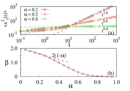
Figure 2: (a) Mean square displacement of the relative motion $x_{r}$ along the shear flow direction for various $\alpha$, with respective line fits. (b) Dependence of $\beta$ on the exponent of subdiffusion $\alpha$. Parameters for the numerical calculation are: $\dot{\gamma}=1,~{}\eta_{\alpha}=1,~{}2k_{B}T=1$ and $\omega_{0}=1$.

$\frac{l}{\alpha(k+l)+2}\approx\frac{l}{2}$, which is expected to hold for small values of $\alpha$, for the first term in Eq. (Transport and tumbling of polymers in viscoelastic shear flow) and the asymptotic forms of $E$ and $E^{(1)}$ regan in the second term, we have:

$$\langle x^{2}_{r}(t)\rangle_{Sh}\sim\frac{\alpha\dot{\gamma}^{2}k_{B}T}{a^{2}\omega^{2}_{0}\Gamma^{2}(2-\alpha)}t^{2-2\alpha}.$$ (7)

This implies that the shear contribution to the motion of the relative coordinate grows without bounds, in a superdiffusive manner ($\alpha$ is small). In addition, as the thermal contribution eventually reaches a steady value, this is the fate of separation between the two masses in that $\langle x^{2}_{r}(t)\rangle\sim t^{\beta}$ with $\beta=2(1-\alpha)$ (for small $\alpha$). For arbitrary values of $\alpha$, such a closed form expression is not possible, and we solve Eq. (5) numerically to assess the behavior of fluctuations in the separation of the two masses. We show the results for $\langle x^{2}_{r}(t)\rangle$ in Fig. 2(a) for different values of $\alpha$. For the entire range of $\alpha\in(0,1)$, Fig. 2(b) shows that the fluctuations in the relative coordinate go from superdiffusive to diffusive to subdiffusive as $\alpha$ grows from 0 to 1supp . The deviation from the straight line behavior is also evident, implying towards the failure of the approximation made to decouple the series in Eq. (Transport and tumbling of polymers in viscoelastic shear flow).

Nonexistence of the steady-state for the motion of relative coordinates implies that the system does not feel the effects of confinement. Hence, the harmonically interacting dumbbell which serves as a starting point for addressing tumbling in viscous shear flows, e.g.- Rouse chains das1 ; das2 , does not work for motion in viscoelastic medium under shear. As a result, we need a potential strong enough to exhibit a nonequilibrium steady state for the motion of relative coordinates. In the next section, we address this problem by introducing nonlinear interactions and study tumbling of dumbbells in viscoelastic shear flows.

Generalized Langevin equation in shear flows-Nonlinear dumbbell model: In order to bring in nonlinearity in the problem, we introduce FENE-LJ potential which is more realistic compared to the harmonic interaction grest . The inter-particle interaction is a contribution from both repulsive and attractive parts, viz. $V=V_{LJ}+V_{FENE}$, wherein

$$V_{LJ}(r)=4\varepsilon[(\sigma/r)^{12}-(\sigma/r)^{6}],~{}\text{and}$$ (8a)

$$V_{FENE}(r)=-(kR^{2}_{0}/2)\ln[1-(r/R_{0})^{2}].$$ (8b)

As mentioned earlier, we consider only the repulsive part of $V_{LJ}$. In above equations, $r=|{\bf r}_{1}-{\bf r}_{2}|$ denotes the separation between the two monomers, $\sigma$ their size, $\varepsilon$ the strength of repulsion, $R_{0}$ the maximum extension, and $k$ the stiffness constant. The force on particle $i$ due to $j$ is $-\nabla_{i}V(|{\bf r}_{i}-{\bf r}_{j}|)$, with $i,j=1,2$. The resulting equations of motion read:

$$\ddot{\bf r}_{i}+\int^{t}_{0}dt^{\prime}\eta(t-t^{\prime})(\dot{\bf r}_{i} -\dot{\gamma}y_{i}{\bf i})(t^{\prime})$$

$$=-\nabla_{i}V(|{\bf r}_{i}-{\bf r}_{j}|)+\dot{\gamma}\dot{y}_{i}{\bf i}+{\bf\xi}_{i}(t),$$ (9)

with $i,~{}j=1,2$ and $i\neq j$. We have retained the acceleration terms for the nonlinear system because of its numerical advantage (avoids root finding like in the overdamped case) supp . The second term on the right hand side of the above equations, $\dot{\gamma}\dot{y}_{i}$ is the coordinate dependent contribution from the flow. This term arises when we take account of the local streaming velocity alongwith the actual momentum mcphie .

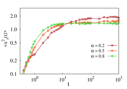
Figure 3: Mean square displacement of relative separation $x_{r}$ of two particle connected by a nonlinear spring for different values of $\alpha$.

Similar to the case of overdamped motion, the center of mass for underdamped motion also follows $\langle x^{2}_{c}(t)\rangle\sim t^{\alpha+2}$. The nonlinear spring, however, unlike the harmonic spring, achieves a steady-state owing the FENE-LJ potential which keeps the bond-length in the interval $(\sigma,R_{0})$. This is evident from the behavior of the mean square displacement $\langle x^{2}_{r}(t)\rangle$ of the relative separation between the two masses connected by the nonlinear spring (cf. Fig. 3).

In what follows, energy is measured in units of $\varepsilon$ and distance in units of $\sigma$. In addition, following kremer ; sdhn , we choose: $\varepsilon=1$, $\sigma=1$, $R_{0}={1.5\sigma}$, $k=30\varepsilon/\sigma^{2}$, $k_{B}T=1.2\varepsilon$ and $\eta_{\alpha}=7.5$.

Distribution of tumbling times:

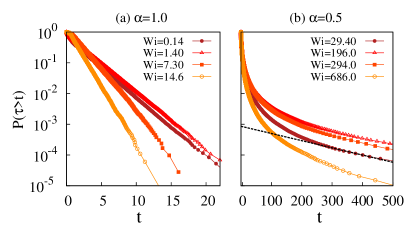
Figure 4: Probability distribution $P(\tau\geq t)$ for the dumbbells tumbling in (a) purely viscous shear flow ($\alpha=1$) vs (b) viscoelastic shear flows ($\alpha=0.5$). The exponentially decaying tails for the two cases are discernible from the graphs (line fit for Wi$=29.40$), with the distributions of the form $P(\tau\geq t)\approx\exp(-\nu\tau)$. In addition, a change in the trend of slope for the two types of flows is also clearly evident.

Tumbling time $\tau$ is defined as the interval of successive zero-crossings of the end-to-end vector $R_{x}=x_{1}-x_{2}$. The distribution of tumbling times $P(\tau\geq t)$ in purely viscous flow exhibits exponentially decaying tails for various values of the Weissenberg number Wi (Fig. 4 (a)). Interestingly, even for tumbling in viscoelastic shear flow, $P(\tau\geq t)$ exhibits exponentially decaying tails (cf. Fig. 4 (b)), though the time $\tau$ taken for the viscoelastic case is much longer when compared to its viscous counterpart. In addition, the tumbling events for the two types of flows, viz. viscous and viscoelastic case occur at different levels of flow strengths. As a matter of fact, the observed values of flow strength for the viscoelastic case are well beyond the experimentally observed ranges for the case of viscous shear flows. This is evident from the respective values of Wi for the two cases, which are at least an order of magnitude apart. The reason for this difference is that relaxation time in a viscoelastic medium is much longer compared to relaxation in a purely viscous fluid. In other words, the effect of viscoelasticity in the medium is to slow down the characteristic tumbling frequency at finite Wi consistent with earlier studies 1 ; 2 ; 3 for rotational dynamics of suspended particle in viscoelastic shear flow. The exponentially decaying tails of the tumbling time distribution, $P(\tau\geq t)\approx\exp(-\nu\tau)$, define the characteristic tumbling time $\tau_{tumb}$ as inverse of the characteristic exponent $\nu$. In addition, for the case of purely viscous flows, i.e.- for $\alpha=1$, we find via numerical calculations that $\nu\tau_{0}\approx\text{Wi}^{0.67}$ for Wi $\gg 1$ celani , wherein $\tau_{0}$ is relaxation time of the autocorrelation $\langle R_{x}(t)R_{x}(t+T)\rangle$.

Effect of subdiffusion on tumbling:

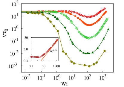
Figure 5: Limiting decay rate $\nu$ scaled with $\tau_{0}$ vs Wi for subdiffusive case for different values of $\alpha$. For weak flow strengths, i.e. for Wi $\ll 1$, the different curves trace each other. On the other hand, for Wi $\gg 1$, the $\nu\tau_{0}$ grows with the Weissenberg number as Wi^μ(α), where the exponent $\mu$ depends on $\alpha$. Inset shows the variation of dimensionless tumbling frequency $\nu\tau_{0}$ with the Weissenberg number Wi for a dumbbell tumbling in a purely viscous medium ($\alpha=1$).

We study the effect of subdiffusion on tumbling of dumbbells in Fig. 5, wherein we find that $\nu\tau_{0}$ exhibits a nonmonotonic behavior with Wi which is absent in viscous medium (cf. inset of Fig. 5). Though there is a slight deviation in the trends of the curve for distribution with increasing Wi (cf. Fig. 4 (a) for $\alpha=1$) showing nonmonotonicity in value of $\nu$ but it is negligible compared to the case for $\alpha<1$. To understand this behavior of $\nu\tau_{0}$ vs Wi, let us have a look at Eq. (Transport and tumbling of polymers in viscoelastic shear flow), from where it is clear that the relative coordinate ${\bf r}_{1}-{\bf r}_{2}$ follows the motion of a single particle in the potential $V=V_{FENE}+V_{LJ}$, and in the absence of shear relaxes at its natural time scale dictated by the parameters of the potential and the degree of subdiffusion $\alpha$. However, when a small but finite amount of shear flow is introduced, it tends to align the dumbbell along the flow. With an increase in the strength of flow, a feedback from the elastic force which tends to preserve the previous relaxation, results in an enhanced tumbling time. Thus, resulting in a decrease in the tumbling frequency $\nu\tau_{0}$ for small Wi. On the other hand, for strong flow, when Wi is quite large, tumbling occurs more frequently due to the increase in the rotational component of shear force dominating the tumbling dynamics. Consequently, for some intermediate value of Wi, the tumbling frequency $\nu\tau_{0}$ hits a minima and our numerical calculations also corroborate this fact.

We also learn from Fig. 5 that the tumbling time $\nu\tau_{0}$ changes significantly at any given value of Wi even for slight decrease in the value of $\alpha$. This is because the fluctuations in the relative coordinate are reduced for low values of $\alpha$, thus making tumbling a flow dominant phenomena which tends to keep the dumbbell oriented along the flow, hence the increase in tumbling time. Interestingly, for viscoelastic case, the increase in $\nu$ starts at quite a high value of Wi as compared to the viscous case. This shift is consequent of the prolonged relaxation in viscoelastic medium due to inherent elasticity.

Now, in the limit of very large values of the Weissenberg number, i.e.- for Wi$\gtrapprox 100$ for which $\nu\tau_{0}$ is observed to monotonically increase with Wi with exponent close to 0.67 ($\alpha=1$) as $\alpha$ approaches unity. However, for arbitrary values of $\alpha$ we have not been able to extract reliable statistics of tumbling times so as to furnish a value of the growth exponent defining the scaling behavior: $\nu\tau_{0}\approx\text{Wi}^{\mu(\alpha)}$ supp . This is because with decreasing $\alpha$, a tumbling event becomes rare to observe making it computationally very challenging to record them in a finite amount of computational time available to us.

Conclusion: Viscoelasticity is more of a rule rather than exception, and motivated by this, we have studied in this paper the transport and tumbling properties of polymers in a viscoelastic fluid under shear. Using dumbbells as representative, we provide analytical results for the motion of center of mass and separation between the two masses. For the simplest case of a harmonic spring connecting the two masses, we that the mean square displacement of the center of mass follows: $\langle x^{2}_{c}(t)\rangle\sim\dot{\gamma}^{2}t^{\alpha+2},~{}0<\alpha<1$, generalizing the earlier result: $\langle x^{2}_{c}(t)\rangle\sim\dot{\gamma}^{2}t^{3}~{}(\alpha=1)$. On the other hand, fluctuations in the relative coordinate also grow monotonically with time, with $\langle x^{2}_{r}(t)\rangle\sim t^{\beta}$, where $\beta=2(1-\alpha)$ up to $\alpha\approx 0.25$ and approaches 0 as $\alpha$ approaches unity. Consequently, the system of two masses connected by a harmonic spring does not achieve a steady-state. In other words, the extensively studied Rouse polymer is inappropriate to address the dynamics of polymers in viscoelastic medium under shear. We remedy this pathology by introducing a nonlinear spring in the form of FENE-LJ interaction which restricts the separation of the two masses to a maximum allowed limit. Employing the nonlinearity in the system we address tumbling of dumbbells and find that the effect of viscoelasticity in medium is to slow down the characteristic tumbling frequency at finite Wi. We hope that our work motivates further studies along this direction, particularly the effect of hydrodynamic interactions on tumbling aspects.

- (1) J. C. Maxwell, Philos. Trans. R. Soc. Lond. 157, 49 (1867).
- (2) R. S. Lakes, Viscoelastic Solids (CRC Press, Boca Raton, 1999).
- (3) R. A. L. Jones, Soft Condensed Matter (Oxford University Press, Oxford, 2002).
- (4) J.-H. Jeon and R. Metzler, Phys. Rev. E 81, 021103 (2010).
- (5) B. B. Mandelbrot and J. W. van Ness, SIAM Rev. 10, 422 (1968).
- (6) J. Szymanski and M. Weiss, Phys. Rev. Lett. 103, 038102 (2009).
- (7) S. C. Weber, A. J. Spakowitz, and J. A. Theriot, Phys. Rev. Lett. 104, 238102 (2010).
- (8) I. Bronstein, Y. Israel, E. Kepten, S. Mai, Y. Shav-Tal, E. Barkai, and Y. Garini, Phys. Rev. Lett. 103, 018102 (2009).
- (9) D. E. Smith, H. P. Babcock, and S. Chu, Science, 283 1724 (1999); and references therein.
- (10) P. LeDuc, C. Haber, G. Bao, and D. Wirtz, Nature 399, 564 (1999).
- (11) F. B. Usabiaga and R. Delgado-Buscalioni, Macromol. Theory Simul. 20, 466 (2011).
- (12) C. M. Schroeder, R. E. Teixeira, E. S. G. Shaqfeh, and S. Chu, Phys. Rev. Lett. 95, 018301 (2005).
- (13) R. G. Winkler, Phys. Rev. Lett. 97, 128301 (2006).
- (14) N. Özkaya and M. Nordin, Fundamentals of Biomechanics pp. 195-218, Springer, New York (1999).
- (15) M. Herrchen and H. C. Öttinger, J. Non-Newtonian Fluid Mech. 68, 17 (1997).
- (16) K. Kremer and G. S. Grest, J. Chem. Phys. 92, 5057 (1990).
- (17) R. Zwanzig, J. Stat. Phys. 9, 215 (1973).
- (18) R. Kubo, Rep. Prog. Phys. 29, 255 (1966).
- (19) P. E. Rouse, J. Chem. Phys. 21, 1272 (1953).
- (20) U. Weiss, Quantum Dissipative Systems, 2nd ed. (World Scientific, Singapore, 1999).
- (21) R. Kupferman, J. Stat. Phys. 114, 291 (2004).
- (22) A. Gemant, Phys. 7, 311 (1936).
- (23) I. Goychuk, Phys. Rev. E 80, 046125 (2009).
- (24) K. G. Wang and M. Tokuyama, Physica A 265, 341 (1999).
- (25) M.G. McPhie, P.J. Daivis, I. K. Snook, J. Ennis and D.J. Evans, Physica A 299, 412 (2001).
- (26) See Supplementary Information details of the numerical calculations.
- (27) I. Goychuk, Adv. Chem. Phys. 150, 187 (2012).
- (28) A. D. Viñales and M. A. Despósito, Phys. Rev. E 73, 016111 (2006).
- (29) M. A. Despósito and A. D. Viñales, Phys. Rev. E 77, 031123 (2008).
- (30) M. A. Despósito and A. D. Viñales, Phys. Rev. E 80, 021111 (2009).
- (31) I. Podlubny, Fractional Differential Equations, Academic Press (1999).
- (32) J. R. Wang, Y. Zhou, and D. O’Regan, Integral Transforms and Special Functions 29, 91 (2018).
- (33) S. Bhattacharya, D. Das, and S. N. Majumdar, Phys. Rev E 75, 061122 (2007).
- (34) D. Das and S. Sabhapandit, Phys. Rev. Lett. 101, 188301 (2008).
- (35) G.S. Grest and K. Kremer, Phys. Rev. A 33, 3628 (1986).
- (36) S. Singh and S. Kumar, J. Chem. Phys. 150, 024906 (2019).
- (37) G. D’Avino, N. A. Hulsen, K. Snijkers, N. Vermant, O. Greco and P. L. Maffettone, J. of Rheology 52, 1331 (2008).
- (38) F. Snijkers, G. D’Avino, R. A. Maffettone, O. Greco, M. Hulsen and J. Vermant, J. of Rheology 53, 459 (2009).
- (39) K. D. Housiadas and R. I. Tanner, Phys. Fluids 30, 073101 (2018).
- (40) A. Celani, A. Puliafito and K. Turitsyn, Europhys. Lett., 70, 464 (2005).