Skyrmion interactions and lattices in chiral magnets: Analytical results

Abstract

We study two-body interactions of magnetic skyrmions on the plane and apply them to a (mostly) analytic description of a skyrmion lattice. This is done in the context of the solvable line, a particular choice of a potential for magnetic anisotropy and Zeeman terms, where analytic expressions for skyrmions are available. The energy of these analytic single skyrmion solutions is found to become negative below a critical point, where the ferromagnetic state is no longer the lowest energy state. This critical value is determined exactly without the ambiguities of numerical simulations. Along the solvable line the interaction energy for a pair of skyrmions is repulsive with power law fall off in contrast to the exponential decay of a purely Zeeman potential term. Using the interaction energy expressions we construct an inhomogeneous skyrmion lattice state, which is a candidate ground states for the model in particular parameter regions. Finally we estimate the transition between the skyrmion lattice and an inhomogeneous spiral state.

1 Introduction

Magnetic skyrmions are topologically non-trivial solitons which occur in certain magnetic materials NT . They were first predicted in BY as minimum energy configurations of the magnetisation vector field and have been observed in a variety of magnetic materials YOKPHMNT ; MBJPRNGB ; RHMBWVKW . In contrast to the case of baby skyrmions – field theoretical analogues of magnetic skyrmions stabilised by higher derivative terms in the energy PSZ ; MS magnetic skyrmions are stabilised by a first order Dzyaloshinskii-Moriya (DM) interaction term (with coefficient $\kappa$) Dzyaloshinskii ; Moriya . The fact that the DM term can give a negative contribution to the energy avoids a contradiction with the usual Derrick scaling argument MS . A systematic mathematical study of magnetic skyrmions in the presence of an external magnetic field and without anisotropy is given in Melcher . The various phases of a chiral magnet have been explored with easy plane anisotropy in addition to an external magnetic field LSB ; BRER ; APL_thinfilms_2016 ; MRG_2016 . The skyrmion lattice phase has been studied extensively in BH ; RBP . A model of a skyrmion lattice made up of non interacting closely packed skyrmions has been considered in HZZJN . Spiral or helical states have also been studied as effectively one-dimensional inhomogeneous states KO2015 ; TOPSK_2018 .

Apart from ground breaking experimental studies YOKPHMNT ; MBJPRNGB ; RHMBWVKW , almost all theoretical studies of magnetic skyrmions are based on numerical simulations thus far and more analytic understanding was lacking. On the other hand, recently in Ref. BRS a specific potential, a combination of a Zeeman term (with coefficient $B$) and an easy plane term (with coefficient $A$), was considered which results in a solvable model for skyrmions in chiral magnetic thin films. More explicitly, tuning the two coefficients of the potential to be $B=2A$, one obtains exact hedgehog skyrmion solutions with topological charge (degree as a mapping $S^{2}\to S^{2}$) $Q=-1$. This relation $B=2A$ of parameters is called the solvable line. These exact skyrmion solutions are a natural generalisation of the ferromagnetic skyrmions in the Heisenberg model BP . The holomorphic properties of the skyrmion solutions along the solvable line were first discussed in MD2016 . While the anisotropy, $A$, and the DM constant, $\kappa$, are determined by the material the external magnetic field, $B$, can be tuned. This suggests that the solvable line should be accessible in real materials through a careful tuning of the external magnetic field.

Along the solvable line $B=2A$, there is a special point tuned to the coefficient $\kappa$ of the DM interaction through $B=2A=\kappa^{2}$. This is a so-called Bogomol’nyi-Prasad-Sommerfield (BPS) Bogomolny:1975de ; Prasad:1975kr point where the model has an infinite number of analytic solutions constructed in terms of holomorphic functions. Such BPS limits were first discussed in the context of monopoles in quantum field theories, and are now known to appear in various theories admitting topological solitons MS , in particular in supersymmetric field theories (see, e. g., Eto:2006pg ; Shifman:2009zz ). In the case of superconductors, it corresponds to the critical coupling between type-I and type-II superconductivities. Some further studies of BPS magnetic skyrmions and instantons in chiral magnets have been made in Refs. Adam:2019yst ; Adam:2019hef ; Hongo:2019nfr .

The exact skyrmion solution along the solvable line reveals the subtlety that a boundary contribution to the energy functional is required for the DM interaction term to be well defined BRS ; Schroers4 ; Schroers5 . This boundary contribution is closely related to the slow power law asymptotic decay of the magnetisation vector for the skyrmion solution. This boundary contribution can give a negative contribution to the energy of the exact skyrmion solution, which can result in the skyrmion having lower energy than the homogeneous ferromagnetic state. This fact opens up the possibility of understanding the inhomogeneous ground state, such as skyrmion lattice states, if a balance is met between the negative energy of individual skyrmions and the interaction energy between them. It is worth emphasising that exact single skyrmion solutions are only known for the solvable line and not for the better studied region $B>2A$. Outside the solvable line, such as for $B>2A$, numerical analysis is needed to construct skyrmion solutions.

The asymptotic decay of the skyrmion fields is also a key difference with a power law decay for the solvable line and an exponential decay for $B>2A$. The slower, power law, decay for skyrmions along the solvable line mean that the asymptotic methods used for $B>2A$ are not as easily applicable. This is because boundary terms in the energy, which vanish for exponential decay, play an important role along the solvable line. Even though $B=2A$ has the subtlety of boundary terms, the presence of exact solutions overrides this disadvantage.

The interaction energy between a pair of skyrmions was discussed for a specific easy-axis potential in Bogdanov1995 and has recently been discussed LRSB_2013 ; CGC ; BLH , using the dipole approximation introduced in Ref. PSZ . Most previous work, including Refs. CGC ; BLH , only considers the case of an external magnetic field without an anisotropy term. It has been found that the interaction energy decays exponentially at large separations in this case FKATDS . The case of easy plane anisotropy being more important than the Zeeman term was considered in Ref. LK2017 where an attractive interaction was found between individual skyrmions. The skyrmion interaction energy for the solvable line does not appear to have been studied before. The boundary contributions to the energy caused by the slow, power law, decay of the skyrmion configurations complicate the asymptotic approach used for $B>2A$. This necessitates a slightly different approach which is possible due to the presence of analytic skyrmion solutions.

In this paper we conduct a semi-analytic study of interactions between magnetic skyrmions along the solvable line, and apply it to construct a model of a skyrmion lattice. To achieve this, we make use of the dipole approximation from PSZ . This approximation involves working with a superposition of two skyrmions, and is reliable as long as the skyrmions are well separated, becoming less reliable as the distinction between the constituent skyrmions becomes less pronounced. The accuracy of the approximation should be measured in terms of the separation between two skyrmions divided by the diameter of a single skyrmion. The diameter of the skyrmion is determined by three dimensionful parameters, the DM interaction strength $\kappa$, and the two parameters $A$ (for magnetic anisotropy) and $B$ (for a Zeeman field) in the potential. From the numerical study of the phase diagram of a chiral magnet with easy plane anisotropy, LSB ; BRER , it is known that large values of $A$ and $B$ correspond to homogeneous ferromagnetic phases. The solvable line, $2A=B$, lies along the phase boundary between the polarised ferromagnetic phase and the spin canted ferromagnetic phase. At large values of the potential along the solvable line, magnetic skyrmions are obtained as positive energy excited states on top of the ferromagnetic ground state. The skyrmions have smaller radii as the potential parameter $A$ becomes larger. Thus the dipole approximation, at a fixed separation between two isolated skyrmions, works best as the potential parameter $A$ becomes large. For small values of $A$, on the other hand, the skyrmions along the solvable line have negative energy and the homogeneous ferromagnetic state becomes unstable. This leads to the possibility of the ground state being an inhomogeneous skyrmion lattice in agreement with numerical studies BH ; RBP . The other possible inhomogeneous state is a spiral or helical state KO2015 ; TOPSK_2018 where the configuration is effectively one dimensional.

We apply the dipole approximation at smaller values of $A$ to understand some of the qualitative behaviour of the triangular skyrmion lattice phase from LSB along the solvable line. We take two exact single skyrmion solutions and consider their superposition as a function of their separation. Our results show that the dipole approximation can be used reliably to find the transition between the ferromagnetic phase and the lattice phase. However, the dipole approximation breaks down before we can study the phase transition between the lattice phase and the spiral phase. We find evidence that a model of a skyrmion lattice as, effectively, non interacting closely packed skyrmions HZZJN becomes a better approximation. Using this we estimate the critical value of the external magnetic field where the transition to the spiral phase occurs.

The key feature of the present work is that by working on the solvable line there are exact expressions for the skyrmion configurations enabling us to make exact statements about the energy of a single skyrmion. This makes it possible for us to identify a specific value of the anisotropy below which the single skyrmion solution has negative energy and we have a state lower in energy than the ferromagnetic state. Combining the exact single skyrmion configurations with the dipole approximation we arrive at an analytic expression for the interaction energy density of the superposition without the need to work asymptotically. After numerical integration we find that the interaction energy is positive and has a power law decay in contrast to the exponential decay of the pure Zeeman potential FKATDS ; CGC ; BLH . An exponentially decaying interaction was also found in Bogdanov1995 for the case of a specific easy-axis potential. Comparing these previous studies with our Appendix A, we see that the interaction energy will exponentially decay when the skyrmion field decays exponentially. Two-body and three-body skyrmion interactions in the absence of an anisotropy term in the potential have been studied in TSA2019 . We show that the power law decay of the skyrmion fields necessitates the inclusion of a boundary term in the energy functional in order to have a well defined variational problem when deriving the equations of motion. Along the solvable line, we find a repulsive interaction.

This paper is organized as follows. In Sec. 2, we review solvable models for magnetic skyrmions and clarify the necessity of a boundary term. In Sec. 3, we calculate the interaction energy and force between two isolated skyrmions. In Sec. 4, the interaction energy is applied to describe a skyrmion lattice, and the phase transition to the spiral phase is estimated. Sec. 5 is devoted to a summary and discussion. Appendix A gives the details of the boundary term in the energy functional and its relation to the asymptotic behaviour of the magnetisation vector field. In Appendix B we express the interaction energy as a function of dimensionless variables. Spiral states are described in Appendix C.

2 Solvable models for magnetic skyrmions

In this section, we review solvable models for magnetic skyrmions. In Subsec. 2.1, we introduce the model and classify homogeneous ground states, when the DM term can be neglected. Then in Subsec. 2.2, we present exact skyrmion solutions. Finally in Subsec. 2.3, we discuss the instability of the ferromagnetic phase.

2.1 The model

This subsection gives a concise summary of previously known results that are directly relevant for our study and clarifies our conventions at the same time. We study chiral magnets in two spatial dimensions described in terms of a real three component magnetisation vector field $\vec{n}:\mathbb{R}^{2}\to S^{2}$, constrained as $\vec{n}^{2}=1$. In works such as BY ; BH ; LSB the following energy functional is considered

$$E[\vec{n}]_{\rm bulk}=\int_{\mathbb{R}^{2}}\left[\frac{1}{2}|\nabla\vec{n}|^{2}+\kappa\;\vec{n}\cdot\left(\nabla_{-\alpha}\times\vec{n}\right)+U(n_{3})\right]d^{2}x,$$ (1)

where the potential $U$ consists of a Zeeman term with the magnetic field $B$ as coefficient, and an anisotropy term with the coefficient $A$

$$U(n_{3})=-Bn_{3}+An_{3}^{2}.$$ (2)

The term corresponding to the parameter $\kappa$ is the Dzyaloshinskii-Moriya (DM) interaction energy Dzyaloshinskii ; Moriya , and the rotated derivative is defined as

$$\nabla_{-\alpha}=\left(\begin{array}[]{c}\cos\alpha\partial_{1}+\sin\alpha\partial_{2}\\ -\sin\alpha\partial_{1}+\cos\alpha\partial_{2}\\ 0\end{array}\right),$$ (3)

where the parameter $\alpha\in[0,2\pi)$ denotes a one parameter family of models corresponding to different types of DM term, for example $\alpha=0$ corresponds to the Bloch type DM and $\alpha=\frac{\pi}{2}$ corresponds to the Néel type DM interaction. The subscript “bulk” indicates that we need to add a boundary term to properly define the DM interaction term (to apply the variational principle), as we describe subsequently.

For large values of the potential parameters $|A|,|B|\gg\kappa$, for which the DM term can be neglected, the ground state is determined by the minimum of the potential. There are three types of minima of the general potential $U(n_{3})$ depending on values of $A,B$:

1. $|B|<2A$: canted ferromagnetic phase ($n_{3}=\frac{B}{2A}$),

2. $B>2A,\,B>0$: Ferromagnetic phase ($n_{3}=+1$),

3. $B<-2A,\,B<0$: Ferromagnetic phase ($n_{3}=-1$).

These three phases exhaust the possible homogeneous ground states. The phase diagram for the ground states of the potential is included in Figure 1.

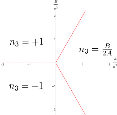
Figure 1: The three ferromagnetic phases of the potential $U(n_{3})=-Bn_{3}+An_{3}^{2}$.

Let us note that the model is invariant under the transformation

$$B\to-B,\quad n_{3}\to-n_{3}.$$ (4)

We consider the parameter region $B\geq 0$ in the following, since we can obtain identical result for $B<0$ by just changing the sign of $n_{3}$.

If we tune the parameters $A,B$ in the potential as

$$B=2A,$$ (5)

(and add a constant $A$), we obtain a potential $V(n_{3})$ instead of $U(n_{3})$ (in the case of $B<0$, we should tune $-B=2A$ to obtain a potential $V(n_{3})=A\left(1+n_{3}\right)^{2}$ instead)

$$V(n_{3})=A\left(1-n_{3}\right)^{2}.$$ (6)

We call this choice of parameters, $B=2A$, the solvable line, since explicit skyrmion configurations can be constructed as shown in the next subsection.

Instead of the constrained vector field $\vec{n}$ with $\vec{n}^{2}=1$, it is often more convenient to use the unconstrained complex field $w$ defined by the stereographic projection

$$w=\frac{n_{1}+in_{2}}{1+n_{3}}.$$ (7)

The energy functional in Eq. (1) with the potential replaced by $V$ in Eq. (6) is rewritten as

$$E[w]_{\rm bulk}^{B=2A}=\int_{\mathbb{R}^{2}}\frac{2|\nabla w|^{2}+4\kappa{\rm Im}(e^{i\alpha}(\partial_{z}w+w^{2}\partial_{z}\bar{w}))+4A|w|^{4}}{(1+|w|^{2})^{2}}d^{2}x.$$ (8)

2.2 Exact single skyrmion solutions

Defining isolated skyrmion states requires knowledge of the minima of the potential. This is because the magnetisation vector of the skyrmion configuration is required to go to the ground state asymptotically.

In the case of derivative interactions like the DM term, particular care is needed to properly define the energy functional. When varying fields to obtain field equations, we need to integrate by parts, which produces a surface term. If the fields do not decay sufficiently fast asymptotically, the surface term obstructs the variational principle used to obtain the field equation. Hence it is mandatory to subtract a boundary term to remove this obstruction and allow us to apply the variational principle. In the case of the DM interaction, this is accomplished by adding the following boundary term Schroers4 ; Schroers5 to the energy functional (1)

$$-4\pi\Omega[\vec{n}]=-\kappa\int_{\mathbb{R}^{2}}\vec{n}_{\infty}\cdot\left(\nabla_{-\alpha}\times\vec{n}\right)d^{2}x.$$ (9)

Here $\vec{n}_{\infty}$ is the asymptotic value of $\vec{n}$ determined by the homogeneous state. Explicitly, for the ferromagnetic phases, $\vec{n}_{\infty}=\pm e_{3}$ with the top sign when $B$ is positive and the lower sign when $B$ is negative.

We wish to stress that only by adding the boundary term, does the DM term become well-defined in terms of the variational problem for the energy functional. More details about the necessity of the boundary term are discussed in Appendix A. Some properties of the boundary term in Eq. (9), are discussed in Refs. BRS ; Melcher .

Taking into account the boundary term in Eq. (9) and the potential in Eq. (6), the model of a chiral magnet that we consider is

$$E[\vec{n}]=E_{\rm bulk}^{B=2A}-4\pi\Omega=\int_{\mathbb{R}^{2}}\left[\frac{1}{2}|\nabla\vec{n}|^{2}+\kappa\;\left(\vec{n}-e_{3}\right)\cdot\left(\nabla_{-\alpha}\times\vec{n}\right)+V(n_{3})\right]d^{2}x.$$ (10)

The tuning of the potential allows one to obtain exact solutions of a hedgehog type BRS . In terms of the polar coordinates $x_{1}=r\cos\varphi$, $x_{2}=r\sin\varphi$, one finds the exact solution by imposing a boundary condition $\vec{n}\to(0,0,1)$ at infinity $r\to\infty$,

$$\vec{n}=\begin{pmatrix}\sin\Theta\cos\left(\varphi+\gamma\right)\\ \sin\Theta\sin\left(\varphi+\gamma\right)\\ \cos\Theta\end{pmatrix}$$ (11)

with phase $\gamma=\frac{\pi}{2}-\alpha$ and profile function

$$\Theta=2\arctan\left(\frac{\kappa}{Ar}\right).$$ (12)

The hedgehog solution is called a skyrmion. It gives a mapping from the base space ${\mathbb{R}^{2}}$ to the target space $S^{2}$. As $\vec{n}$ tends to a constant as $r\to\infty$ we can regard ${\mathbb{R}^{2}}$ as $S^{2}$ by adding the point at infinity, thus we can define the degree $Q$ corresponding to $\pi_{2}(S^{2})$

$$Q[\vec{n}]= \frac{1}{4\pi}\int\vec{n}\cdot\partial_{1}\vec{n}\times\partial_{2}\vec{n}\;d^{2}x.$$ (13)

This topological charge is $Q=-1$ for a skyrmion configuration. It is worth repeating that in this context a skyrmion has topological charge $Q=-1$ while an anti-skyrmion has topological charge $Q=+1$. This is in contrast to the case of baby skyrmions as discussed in MS .

The skyrmion solution has energy

$$E=4\pi\left(1-\frac{\kappa^{2}}{A}\right).$$ (14)

Here, when calculating the energy of the skyrmion, taking into account the boundary term (9) is crucial. This is an exact expression for the skyrmion energy as a function of $\frac{A}{\kappa^{2}}$ along the solvable line. The analytic skyrmion solutions, Eqs. (11) and (12), along the solvable line enable us to compute this exact energy expression. As highlighted in Table 1, subtracting the boundary term leads to the skyrmion having negative energy which is very important for our approach to constructing the skyrmion lattice.

Table 1: A table comparing the energy of the exact skyrmion solution and BPS anti-skyrmion with and without the boundary term, Eq. (9). The BPS case is $B=2A=\kappa^{2}$ and the anti-skyrmion is constructed from Eq. (21) with $f(z)=z$. Subtracting the boundary term is necessary for the skyrmions to have negative energy.

	Skyrmion	BPS skyrmion	BPS anti-skyrmion
$E_{\rm bulk}^{B=2A}$	$4\pi$	$4\pi$	$4\pi$
$E[\vec{n}]$	$4\pi\left(1-\frac{\kappa^{2}}{A}\right)$	$-4\pi$	$4\pi$

The profile function in Eq. (12) shows that $n_{3}=0$ (the magnetisation vector lies in the $x-y$ plane) at

$$r=\frac{\kappa}{A},$$ (15)

which is defined as the radius of a skyrmion.

In terms of the complex field $w$ of the stereographic projection, the energy functional and topological charge can be expressed as

$$E[w]=4\pi Q+\int_{\mathbb{R}^{2}}\frac{8|\partial_{z}\bar{w}|^{2}+8\kappa{\rm Im}(e^{-i\alpha}w^{2}\partial_{z}\bar{w})+4A|w|^{4}}{(1+|w|^{2})^{2}}d^{2}x,$$ (16)

and

$$Q=\frac{1}{\pi}\int_{\mathbb{R}^{2}}\frac{\partial_{z}w\partial_{\bar{z}}\bar{w}-\partial_{\bar{z}}w\partial_{z}\bar{w}}{(1+|w|^{2})^{2}}d^{2}x,$$ (17)

respectively. The single skyrmion exact solution can be rewritten in terms of the stereographic complex field $w$ in Eq. (7) as

$$w=i\frac{\kappa}{A}\frac{e^{-i\alpha}}{\bar{z}-\bar{b}},$$ (18)

where the centre of the skyrmion is denoted as $z=b$, here $\vec{n}=(0,0,-1)^{T}$.

In Ref. BRS it was shown that for the BPS case ($B=2A=\kappa^{2}$) we can complete the square in the energy functional (10) and find first order BPS equations

$$D_{1}\vec{n}=-\vec{n}\times D_{2}\vec{n},\qquad D_{2}\vec{n}=\vec{n}\times D_{1}\vec{n}$$ (19)

where $D_{i}\vec{n}=\partial_{i}\vec{n}-\kappa e^{-\alpha}_{i}\times\vec{n}$, for $i=1,2$, is a covariant (helical) derivative. In terms of the stereographic field $w$ in Eq. (7), the BPS equations become

$$\partial_{\bar{z}}w=\frac{i}{2}e^{i\alpha}\kappa w^{2},$$ (20)

and there are infinitely many BPS solutions, with topological charge $Q\geq-1$, of the form

$$w=\frac{2i}{e^{i\alpha}\kappa\bar{z}+2if(z)},$$ (21)

for $f(z)$ an arbitrary holomorphic function. Solutions of these BPS equations with the boundary condition $n_{3}\to 1$ at $r\to\infty$ have energy given by their topological charge $E[\vec{n}]=4\pi Q[\vec{n}]=\int\vec{n}\cdot\left(\partial_{1}\vec{n}\times\partial_{2}\vec{n}\right)d^{2}x$. This is in contrast to the usual story for soliton solutions in the familiar $O(3)$ sigma model MS where the energy is given by $4\pi|Q[\vec{n}]|$. The exact Hedgehog solution in Eq. (18) at $2A=\kappa^{2}$ coincides with the BPS solution with $Q=-1$. Full details of these BPS solutions are given in Refs. BRS ; Schroers4 .

2.3 Instability of ferromagnetic phase

We are now in a position to consider the ground state of the chiral magnet described by the energy functional in (10) along the solvable line $B=2A>0$. The solvable line coincides precisely with the boundary between the ferromagnetic ($n_{3}=+1$) and canted ferromagnetic phases. Along the solvable line, we obtain the ferromagnetic ground state $n_{3}=+1$ in the limit $A\to\infty$. If we decrease the potential strength parameter $A$, the DM interaction becomes more important and can result in a negative energy. The exact single skyrmion energy Eq. (14) shows that a single skyrmion is a positive energy excited state above the ferromagnetic ground state for $A>\kappa^{2}$. On the other hand, the negative energy of the exact single skyrmion solution for $A<\kappa^{2}$ reveals that the homogeneous ferromagnetic state is no longer the lowest energy state. As $A$ decreases down to $\kappa^{2}$, we expect that skyrmions will start to appear as defects in the homogeneous ferromagnetic state. Therefore we expect that there is a phase boundary at $A=\kappa^{2}$, below which an inhomogeneous state with many skyrmions is favored over the homogeneous ferromagnetic state. Repeating this for emphasis, the analytic skyrmion solutions become negative energy states for $A<\kappa^{2}$ and thus the ferromagnetic state is no longer the lowest energy solution of the equations of motion. This suggests that there will be a phase transition to a new inhomogeneous ground state constructed from the negative energy skyrmions. This is our first observation of the precise value of the phase transition point in a chiral magnet. This transition point cannot be established precisely by numerical methods and shows the power of the analytical single skyrmion solutions.

Detailed numerical studies LSB ; APL_thinfilms_2016 ; MRG_2016 showed that the inhomogeneous phases are the skyrmion lattice phase, at intermediate values of $A$ below $\kappa^{2}$, and the spiral phase, for the region much below $\kappa^{2}$. In subsequent sections, we wish to shed more light on the nature of these inhomogeneous ground states and their phase boundaries by analytic means, rather than numerically.

As we have an exact expression for the energy (14) and the radius (15) of a skyrmion, we can compute the energy density inside a skyrmion. We assume that the skyrmion energy (14) is approximately contained inside the circle of the skyrmion radius $r=\kappa/A$ with the area $\pi\left({\kappa}/{A}\right)^{2}$. This leads to the skyrmion energy density being

$$\langle e_{\text{Sk}}\rangle=\frac{4\pi\left(1-\frac{\kappa^{2}}{A}\right)}{\pi\left(\frac{\kappa}{A}\right)^{2}}=4A\left(\frac{A}{\kappa^{2}}-1\right).$$ (22)

We observe that the energy density is symmetric around $A=\frac{\kappa^{2}}{2}$.

For values of $A$ higher than $\kappa^{2}$, the energy density is positive. As $A\to\infty$, the single skyrmion energy increases towards $4\pi$ and the skyrmion radius goes to zero. Conversely, the skyrmion radius diverges in the limit $A\to 0$, indicating that the $n_{3}=0$ circle becomes very large and that the region where $n_{3}=-1$ covers most of the interior. In the same limit the energy of a single skyrmion diverges. However, the average energy density (22) goes to zero.

3 Interactions of magnetic skyrmions

Although it is energetically more favorable to produce skyrmions below the phase transition point, one cannot create infinitely many skyrmions because of their interaction. Therefore, it is important to study the interactions between skyrmions in order to understand the inhomogeneous ground state. We can use the method from Refs. PSZ ; FKATDS and consider the case of two $Q=-1$ skyrmions. The centres of the skyrmions are defined to be the points where $n=\begin{pmatrix}0,&0,&-1\end{pmatrix}^{T}$. In this section we explain the approximation and use it to fit the interaction energy as a function of the ratio of separation to the skyrmion diameter for various values of $\frac{A}{\kappa^{2}}$.

3.1 Superpositions of skyrmions

We study the interaction between two magnetic skyrmions of degree $Q=-1$ by constructing a degree $Q=-2$ skyrmion configuration, which approaches a solution of the field equations at infinite separations. In Refs. PSZ ; FKATDS , the magnetisation field $\vec{n}$ is used to superpose two skyrmion solutions, $\vec{n}^{A}$ and $\vec{n}^{B}$. The degree of the superposition is the sum of the degrees of $\vec{n}^{A}$ and $\vec{n}^{B}$, in this case $Q=-2$. Here, we work at the level of the complex field in Eq. (7) where the superposition is

$$w=w_{A}+w_{B}.$$ (23)

The superposition in terms of the complex field has the advantage of automatically satisfying the constraint $\vec{n}^{2}=1$, in contrast to the superposition in terms of $\vec{n}$. The two degree $Q=-1$ fields, $w_{A}$ and $w_{B}$, both solve the equations of motion. However, the superposition $w$ does not as the equations of motion are non-linear. As stated above the superposition becomes a solution only in the limit of infinite separation. Hence the accuracy of the approximation improves as the centres of the skyrmions (the poles of the $w$’s) get further apart. Some examples of these superposition configurations at different values of $A$ are included in Fig. 2. These figures show that as $A$ decreases the approximation becomes less reliable. In fact the key quantity to consider is the ratio of the separation to the skyrmion diameter, this will be made explicit below. For the case $B>2A$ where the skyrmion fields are exponentially decaying, the decay exponent gives a characteristic length scale which controls the validity of the dipole approximation. Along the solvable line the power law decay complicates matters and it is not as obvious how to extract a characteristic length scale. However, it is still known that the superposition approaches a true solution for infinite separation. This means that the accuracy of the approximation will improve with increasing separation. In fact we show below that it is best to work in terms of a dimensionless separation which demonstrates that the accuracy of the approximation also depends on the value of $A$.

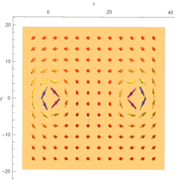
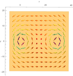
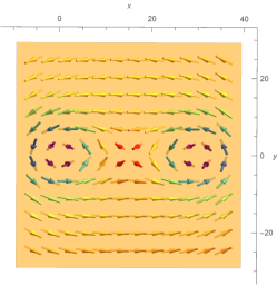
Figure 2: The magnetisation vector field for the superposition of two $Q=-1$ hedgehog skyrmions with one skyrmion centred at zero and the other skyrmion centred at $(30\kappa^{-1},0)$. On the left the plot is for $A=\frac{\kappa^{2}}{2}$, in the middle is $A=\frac{2}{10}\kappa^{2}$, and on the right is $A=\frac{1}{10}\kappa^{2}$. This shows that as $A$ decreases, at fixed separation, the interpretation of the superposition as two distinct skyrmions disappears and the approximation becomes worse.

We take a skyrmion $w_{A}$ centred at the origin and another $w_{B}$ centred at $z=b\in\mathbb{C}$

$$w_{A}=\frac{i\kappa e^{-i\alpha}}{A\bar{z}},\qquad w_{B}=\frac{i\kappa e^{-i\alpha}}{A\left(\bar{z}-\bar{b}\right)}.$$ (24)

The superposition is then given by

$$w=\frac{i\kappa e^{-i\alpha}}{A}\frac{2\bar{z}-\bar{b}}{\bar{z}\left(\bar{z}-\bar{b}\right)}.$$ (25)

This has degree $Q=-2$ for all values of $b$, except $b=0$. At $b=0$ there is a cancellation between the numerator and the denominator and we end up with $w=\frac{2i\kappa e^{-i\alpha}}{A\bar{z}}$, a $Q=-1$ configuration that is not a solution of the equations of motion.

We define the interaction energy of the pair of skyrmions $w_{A},w_{B}$ to be

$$E_{\text{int}}[w]=E[w]-E[w_{A}]-E[w_{B}],$$ (26)

and regard it as the potential energy of the two-body force between the skyrmion pair. Our energy functional $E$ is dimensionless (a dimensionful constant is divided out from the physical energy). With this convention, the interaction energy $E_{\text{int}}[w]$ is also dimensionless. For dimensional reasons, $E_{\text{int}}[w]$ is a function of only two dimensionless ratios of the three dimensionful parameters, $\kappa,A,b$. We define dimensionless coordinates $\zeta,\beta$ as

$$\zeta=\frac{2A}{\kappa}e^{-i\alpha}z,\quad\beta=\frac{2A}{\kappa}e^{-i\alpha}b.$$ (27)

The physical (dimensionful) separation $|b|$ between two skyrmions is given in terms of the dimensionless separation $|\beta|$ as $|b|=|\beta|r/2$. In Appendix B, we show that the interaction energy has the following simple structure as a function of two dimensionless parameters $\beta$ and $\kappa^{2}/(2A)$

$$E_{\text{int}}[w]=\left[\left(\mathcal{I}_{2}^{\text{sup}}\left(|\beta|\right)+16\pi\right)\right]\frac{\kappa^{2}}{2A},$$ (28)

$$\mathcal{I}_{2}^{\text{sup}}\left(|\beta|\right)=\int 2\left(\frac{|w|^{4}+4\text{Im}\left(w^{2}\partial_{\zeta}\bar{w}\right)}{\left(1+|w|^{2}\right)^{2}}\right)d^{2}\zeta.$$ (29)

We observe that the interaction energy is independent of the angle parameter $\alpha$ of the DM interaction, and depends on $\kappa^{2}/(2A)$ only linearly. The coefficient $\mathcal{I}_{2}^{\text{sup}}$ depends only on the magnitude of the dimensionless separation, $|\beta|$.

3.2 Qualitative analysis of interactions

At the BPS point $B=2A=\kappa^{2}$, the interaction energy of the superposition $w$ is positive. This is demonstrated in the following way. The completing the square argument from Ref. BRS can be applied to Eq. (16) with $A=\kappa^{2}/2$. Using the superposition $w$ with the degree $Q=-2$, we obtain

$$E[w]=-8\pi+8\int\frac{\left|\partial_{\bar{z}}w-\frac{i}{2}\kappa e^{i\alpha}w^{2}\right|^{2}}{(1+|w|^{2})^{2}}d^{2}x\geq-8\pi.$$ (30)

The second term is zero when the BPS equations are satisfied and is positive for every other configuration. This means that the energy in the degree $Q=-2$ sector is bounded below by $-8\pi$. Now from the definition of the interaction energy in (26) we have

$$E_{\text{int}}[w]=E[w]-E[w_{A}]-E[w_{B}]=E[w]+8\pi\geq 0,$$ (31)

where we have used that both $w_{A}$ and $w_{B}$ are BPS skyrmions with energy $E=-4\pi$. This means that the interaction energy, $E_{\text{int}}$ must be positive to respect the completing the square argument. We also know that the interaction energy must vanish in the limit of infinite separation. Combining these facts, we find that the interaction is repulsive at least for asymptotically large separations.

It was not known if the interaction energy is positive for other values of $\frac{A}{\kappa^{2}}$. For the range of $A$ which we consider, we find that the interaction energy between the exact skyrmion solutions is always positive.

For general external magnetic fields and anisotropies there are no known exact solutions so a different approach is needed to study the interaction energy. One way to approach this is to consider the asymptotic form of the equation for the hedgehog profile, $\Theta(r)$, as is done for $A=0$ in FKATDS ; BLH . Another approach used in CGC , again for $A=0$, is to proceed numerically. Both of these approaches find that the interaction energy is repulsive and decreases exponentially for increasing separation.

3.3 Computation of the interaction energy

We are now ready to compute the interaction energy between two exact single skyrmion solutions $w_{A}$ and $w_{B}$ in Eq. (24). Our approach proceeds by evaluating Eq. (28) for the superposition $w=w_{A}+w_{B}$. We can assume without loss of generality that $\beta$ is a real parameter. This is because the invariance of the energy under rotations, $w(\xi)\to e^{i\theta}w\left(e^{-i\theta}\xi\right)$, means that the interaction energy just depends on the modulus of the dimensionless separation, $|\beta|$. We compute the integrand of Eq. (29) and numerically integrate it using Mathematica, to find an expression for $E_{\text{int}}[w]$ using Eq. (28). The integration is carried out in a $2\times 10^{6}$ by $2\times 10^{6}$ region so that we can approximate the boundary as being at infinity compared to the skyrmion separation. After repeating the integration at many separations, between $|\beta|=30$ and $|\beta|=500$ we fit the interaction energy as a function of the dimensionless separation $|\beta|$ using a log-log plot and find:

$$\mathcal{I}_{2}^{\text{sup}}\left(|\beta|\right)+16\pi\simeq\frac{1592}{|\beta|^{1.735}}.$$ (32)

The interaction energy is then

$$E_{\text{int}}[w]\simeq\frac{\kappa^{2}}{2A}\frac{1592}{|\beta|^{1.735}}.$$ (33)

The power law fit for $\mathcal{I}_{2}^{\text{sup}}\left(|\beta|\right)+16\pi$ is plotted in Fig. 3. There is good agreement between the fit and the numerical computation for larger separations. At small separations there is a slight deviation with Eq. (33) marginally over estimating the strength of the interaction.

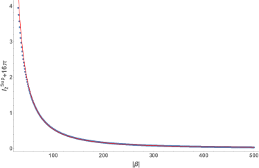
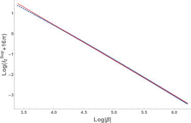
Figure 3: These are fitted plots of $\mathcal{I}_{2}^{\text{sup}}\left(|\beta|\right)+16\pi$ for $30<|\beta|<500$. On the left $\mathcal{I}_{2}^{\text{sup}}\left(|\beta|\right)+16\pi$ is plotted against the dimensionless separation $|\beta|$, while on the right $\log\left(\mathcal{I}_{2}^{\text{sup}}\left(|\beta|\right)+16\pi\right)$ is plotted against $\log|\beta|$. The data points are the numerically computed values of $\mathcal{I}_{2}^{\text{sup}}+16\pi$ and the red fit line is $\frac{1592}{|\beta|^{1.735}}$.

The general trends that we observe are that skyrmions are small, weakly interacting, and have positive energy for large values of $\frac{A}{\kappa^{2}}$. As $A$ decreases towards $\kappa^{2}$, the inter-skyrmion interaction gets stronger and the skyrmions increase in size and decrease in energy, with the energy of an individual skyrmion vanishing at $A=\kappa^{2}$, the phase transition point between the ferromagnetic and skyrmion lattice phases.

The interaction gets stronger and the skyrmion energy becomes more negative as $A$ decreases. On the other hand, the relative separation $|\beta|$ becomes smaller as $\frac{A}{\kappa^{2}}$ decreases. Therefore our results get less reliable as $A$ decreases, and it is likely that we are overestimating the repulsive interaction energy. This can be observed directly from Fig. 2 where for smaller values of $A$ the distinction between the two single skyrmions becomes less pronounced. At short distances, the skyrmions will have a significant effect on each others shape and a more sophisticated method is needed to account for this.

4 Skyrmion lattice states

4.1 Average energy density of skyrmion lattice state

For $A<\kappa^{2}$, the homogeneous ferromagnetic state becomes unstable due to the emergence of negative energy single skyrmion solutions. The negative energy of individual skyrmions results in a preference to produce as many skyrmions as possible. However, the repulsive interaction prevents the skyrmions from becoming too densely packed. This competition is expected to lead to a lattice of skyrmions. Depending on symmetries, either a triangular or square lattice configuration will have the lowest energy. An extensive numerical study in Ref. LSB indicated that a triangular lattice configuration is the ground state for the parameter range where the exact skyrmion solutions occur, as in the case of Abrikosov lattices of vortices in superconductors and superfluids. A cubic lattice of merons, half skyrmions, was also found numerically in another parameter region with larger anisotropy, $B<2A$. In light of this numerical work we construct a simple model for a triangular lattice of skyrmions. Using this model, we compute the average energy per unit cell and find the lattice spacing which minimises this.

Assuming that the two-body force between skyrmions is the dominant interaction, we estimate the average energy density of the triangular lattice state. Let us identify the lattice spacing to be the separation $|b|$ in the calculation of the two-body force between skyrmions in Eq.(24). We find it convenient to use a dimensionless separation $\ell$ defined as the ratio of $|b|$ to the diameter of a single skyrmion $2r=2\kappa/A$

$$\ell=\frac{|b|}{2r}=\frac{|b|A}{2\kappa}=\frac{|\beta|}{4}.$$ (34)

Using the interaction energies computed in the previous section, we now compute the approximate energy density for a triangular skyrmion lattice.

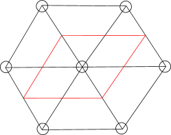
Figure 4: The unit cell of the triangular lattice is the red parallelogram.

Our approach is to compute the energy per unit cell. The unit cell contains one skyrmion, with 6 nearest neighbours, and has area $\frac{\sqrt{3}}{2}|b|^{2}=\frac{\sqrt{3}}{2}(\frac{2\kappa\ell}{A})^{2}$, as shown in Fig. 4. The average energy density is then given by

$$\langle e_{\text{Lattice}}\rangle\left(\ell\right)=\left(\frac{A}{2\kappa}\right)^{2}\frac{2}{\sqrt{3}\ell^{2}}\left(E_{\text{Sky}}+3E_{\text{int}}\right)=\left(\frac{A}{2\kappa}\right)^{2}\frac{2}{\sqrt{3}\ell^{2}}\left(E_{\text{Sky}}+3\frac{\kappa^{2}C_{1}}{2A\ell^{1.735}}\right),$$ (35)

where $E_{\text{Sky}}$ is the skyrmion energy given in Eq. (14), and $C_{1}\simeq\frac{1592}{4^{1.735}}$ is the constant given in Eq. (33) when substituting Eq. (34) for $|\beta|$.

Depending on the value of $\frac{A}{\kappa^{2}}$, Eq. (35) will have different behaviour as a function of $\ell$. In Fig. 5 we plot $\langle e_{\text{Lattice}}\rangle$ as a function of $\ell$ for the BPS case, $\frac{A}{\kappa^{2}}=\frac{1}{2}$, and at the phase transition to the ferromagnetic phase, $\frac{A}{\kappa^{2}}=1$. In the BPS case $\langle e_{\text{Lattice}}\rangle$ is negative at its minimum and there the triangular skyrmion lattice is the ground state. While for $\frac{A}{\kappa^{2}}\geq 1$ the minimum of $\langle e_{\text{Lattice}}\rangle$ is positive and reached for asymptotically separated skyrmions. This is because the ferromagnetic state is the ground state and skyrmions arise as positive energy excitations above it.

When $\frac{A}{\kappa^{2}}<1$ minimising Eq. (35) with respect to $\ell$ leads to $\ell=\ell_{\text{min}}$ with

$$\ell_{\text{min}}\simeq\left(-\frac{\left(2+\delta\right)3C_{1}}{16\pi\left(\frac{A}{\kappa^{2}}-1\right)}\right)^{\frac{1}{\delta}},$$ (36)

where $\delta=1.735$.

The average energy density $\langle e_{\text{Lattice}}\rangle\left(\ell_{\text{min}}\right)$ and the dimensionless lattice spacing at the minimum, $\ell_{\text{min}}$, are plotted against $\frac{A}{\kappa^{2}}$ in Fig. 6 and Fig. 7, respectively. These figures show that as $\frac{A}{\kappa^{2}}$ decreases the dimensionless lattice separation at the minimum decreases. While at first the lattice energy density decreases with decreasing $\frac{A}{\kappa^{2}}$ it reaches a minimum near $\frac{A}{\kappa^{2}}=0.3$ before increasing towards zero.

Let us make a few observations. Firstly we observe that a finite lattice spacing is achieved by the balance between the negative energy of constituent skyrmions and the positive energy due to the repulsive interaction between skyrmions. Secondly, this semi-analytic understanding is most reliable quantitatively for regions near the phase transition point $\frac{A}{\kappa^{2}}=1$. Thirdly for small $\frac{A}{\kappa^{2}}$, $|\beta|$ becomes small. Hence our calculation of the interaction energy becomes less reliable. Since we are using a superposition of single skyrmion solutions as a variational Ansatz for a $Q=-2$ configuration, we naturally expect that the true total energy at a fixed separation, for a $Q=-2$ configuration, may be lower. Namely it is quite likely that our approximate result for the interaction energy is overestimating the repulsive interaction. Therefore we expect that the skyrmion separation in the lattice will be smaller than our estimate for small values of $\frac{A}{\kappa^{2}}$.

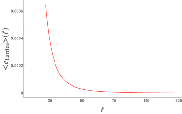
Figure 5: These are plots of the energy per unit cell from Eq. (35). On the left is the critically coupled case $A=\frac{\kappa^{2}}{2}$ with its minimum at $\ell\simeq 11$ and on the right is $A=\kappa^{2}$ whose minimum is for infinitely separated skyrmions.

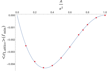
Figure 6: This figure shows how the average energy density of the lattice, (35), at the minimum changes with $A$. The blue line is found by substituting the approximate value of $\ell_{\text{min}}$ from Eq. (36) into Eq. (35) and the red points are found numerically.

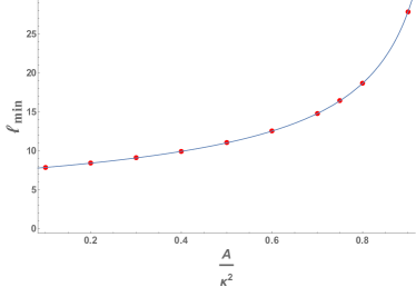
Figure 7: Here we plot the dimensionless lattice separation $\ell_{\text{min}}$ from Eq. (36) against $\frac{A}{\kappa^{2}}$. As $A$ decreases $\ell_{\text{min}}$ also decreases. The blue curve is a plot of the approximate value of $\ell_{\text{min}}$ from Eq. (36) and the red points are the numerically computed values of $\ell_{\text{min}}$.

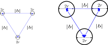
Figure 8: A schematic of showing how the skyrmion diameter $2r$ and the lattice separation $|b|$ change with decreasing $\frac{A}{\kappa^{2}}$. On the left for larger $A$ the lattice spacing, $|b|$ is much larger than the diameter of the skyrmion, $2r$. On the right for lower $\frac{A}{\kappa^{2}}$ both the skyrmion diameter and lattice separation increase but their ratio, $\ell=\frac{|b|}{2r}$, decreases. The scale in the figure on the right has been exaggerated for effect.

4.2 Transition to the spiral state

For smaller values of the parameter $A$, compared to the DM interaction parameter $\kappa^{2}$, we expect from LSB that spiral states have lower energy than the lattice. Thus we expect that a phase transition between the skyrmion lattice and spiral states occurs. As we have seen in the preceding section, our estimate of interaction energy is likely to be an overestimate for smaller values of $\frac{A}{\kappa^{2}}$. On the other hand, the exact single skyrmion solution has energy $E_{\rm Sky}=4\pi(1-\frac{\kappa^{2}}{A})\to-\infty$ and radius $r=\frac{\kappa}{A}\to\infty$ as $A\to 0$, with the average energy density $\langle e_{\text{Sk}}\rangle$ inside the radius tending to a finite value.

From Fig. 7 we see that for small $\frac{A}{\kappa^{2}}$ the lattice spacing and the skyrmion diameter become the same order of magnitude. This suggests that near the transition between the lattice and spiral phases we need a better model of the lattice. As a candidate model of this kind, we consider the case of skyrmions separated by a multiple of the skyrmion diameter,

$$|b|=2c\frac{\kappa}{A}$$ (37)

with $c$ a positive constant. The case of $c=1$ would have skyrmions separated by $2\frac{\kappa}{A}$, the skyrmion diameter, which means that the magnetisation vector $\vec{n}$ will not attain the value $e_{3}$ between the skyrmions. A situation like this is called a hexagonal meron lattice in SKC . As such we are interested in $c>1$ and will in fact focus on $c=2$. We are also assuming that the repulsive skyrmion interaction can be neglected, except to keep the skyrmions from merging, such that they form a lattice. This leads to the situation depicted on the right in Fig. 8. This type of triangular lattice made from nearly touching skyrmions was considered in HZZJN . This scenario seems to be more realistic for small values of $\frac{A}{\kappa^{2}}$, since we are overestimating the interaction energy in that region.

Using this alternative model of a skyrmion lattice we can estimate the value of $A$ that the transition between the lattice phase to the spiral phase occurs at. To do this we note that for $V(n_{3})=0$ (at $A=B=0$) there is an exact spiral solution

$$\vec{n}=\begin{pmatrix}0\\ -\sin\left(\kappa x\right)\\ \phantom{-}\cos\left(\kappa x\right)\end{pmatrix}$$ (38)

with average energy

$$\langle e_{\text{spiral}}\rangle=-\frac{\kappa^{2}}{2}.$$ (39)

The most general spiral solution at $A=B=0$ is obtained by rotating and/or translating this solution in the $x$-$y$ plane with the simultaneous rotation of the magnetization vector $\vec{n}$. This has an identical energy density so we choose to work with the simplest case, Eq. (38). When the potential is non-zero the spiral configuration given by Eq. (38) has average energy

$$\langle e_{\text{spiral}}\rangle=-\frac{\kappa^{2}}{2}+\frac{3A}{2},$$ (40)

which is shown in Appendix C. While it is not a solution of the equations of motion it provides an approximation for a spiral state when the potential is small. In Melcher for $A=0,B\neq 0$ a spiral state like Eq. (38) was motivated by comparing the energy functional Eq. (1) to an energy functional whose ground states are Beltrami fields, solutions to $\nabla\times\vec{n}+\kappa\vec{n}=0$. A rough estimate of where the transition between the skyrmion lattice and the spiral takes place can be found by comparing this to the average energy density of a single skyrmion. The skyrmion average energy is given by Eq. (69). The transition will occur when these two energy densities are equal. When the separation is $|b|=4\frac{\kappa}{A}$ (taking $c=2$ in Eq. (37)) this gives the phase transition at

$$A=\frac{\kappa^{2}}{16}\left(20-4\sqrt{17}\right)\simeq 0.22\kappa^{2},$$ (41)

this value of $A$ matches the location of the phase transition found numerically in LSB . We refer the reader to Appendix C for the explicit details of this computation. At this value of the coupling the spiral state has energy density

$$\langle e_{\text{spiral}}\rangle\simeq-0.17\kappa^{2}.$$ (42)

This energy density is much lower than the energy density that we found for the skyrmion lattice in Fig. 6 using the dipole approximation. This is further evidence that our dipole approximation underestimates the energy density because it is over estimating the interaction energy.

5 Conclusion

In this paper, we have studied the interaction between two well-separated skyrmions and the phase structure of a chiral magnet. We have focused on the solvable line $B=2A$, where $A$ is the anisotorpy parameter and $B$ is the magnetic field parameter in the potential, so that we can make use of the exact skyrmion configurations from Ref. BRS . For $\frac{A}{\kappa^{2}}\gg 1$, where the DM interaction can be neglected compared to the potential, we have found the homogeneous ferromagnetic state $n_{3}=1$ as the ground state. This ferromagnetic phase continues for smaller values of $\frac{A}{\kappa^{2}}$ until we reach the critical point at $\frac{A}{\kappa^{2}}=1$, where the exact skyrmion solution has zero energy. Below this point $\frac{A}{\kappa^{2}}<1$, the exact skyrmion solution has negative energy. The presence of a negative energy solution to the equations of motion means that the homogeneous ferromagnetic state is no longer the lowest energy state. This suggests that the true ground state becomes an inhomogeneous skyrmion lattice state as is found numerically in Ref. LSB ; APL_thinfilms_2016 ; MRG_2016 . As the skyrmion energy is known analytically the transition point, $A=\kappa^{2}$, is found exactly without the ambiguity of numerical simulations. This is only possible on the solvable line where exact skyrmion solutions are known.

We have studied the properties of this skyrmion lattice state by working out the interaction between exact skyrmion configurations along the solvable line $B=2A$. To achieve this we used the dipole approximation for the superposition of two, exact, single skyrmion solutions centred with a finite separation. and have found that the interaction energy is independent of the angle parameter of the DM interaction which distinguishes Bloch, Néel or other types of skyrmion. Exact expressions for the interaction energy density were obtained and after numerically integrating these a power law fit is found for the interaction energy of well separated skyrmions. Using the computed interaction energies, we have been able to predict that the phase transition from a skyrmion lattice state to a ferromagnetic state will happen for $\frac{A}{\kappa^{2}}=1$. Our results have also demonstrated that in the skyrmion lattice phase as $\frac{A}{\kappa^{2}}$ decreases the ratio of lattice separation to the skyrmion diameter decreases. This suggests that near the boundary between the lattice and spiral phases the lattice can be approximately computed by taking the lattice density to be the energy density of a single skyrmion. This allows us to gain a semi-analytic understanding of the phase diagram of a chiral magnet along the solvable line. In particular we determine the location of the phase transition between the homogeneous ferromagnetic phase and the skyrmion lattice phase precisely, and estimated the transition between the skyrmion lattice phase and the spiral phase.

We have emphasized the need for the boundary term in the energy functional to make the DM interaction term well defined, and have clarified its close relation to the asymptotic behavior of the magnetisation vector.

We need to emphasise that our work deals only with static configurations, since the exact skyrmion configurations from Ref. BRS that we have used are minimisers of the static energy functional. Understanding the effect of time evolution of excited states above the ground state is an open problem, which requires an understanding of the dynamics of skyrmion configurations and their superposition. Another interesting open problem is to find the values of $A$ and $B$ at which the single skyrmion energy becomes negative away from the solvable line.

We have studied skyrmions in two dimensions, applicable to a thin film. In three spatial dimensions, skyrmions are lines for which one can study collective modes propagating along a skyrmion line Kobayashi:2014eqa . Extension of the present work to three dimensions remains an open problem.

Appendix A DM interaction and boundary terms

In this appendix, we explain why the inclusion of the boundary term in the energy functional is mandatory. Let us consider the energy functional $E[\vec{n}]_{\rm bulk}$ in the bulk with the DM interaction in Eq. (1). To obtain the equation of motion by the variational principle, we consider a variation of the bulk energy functional $\delta E[\vec{n}]_{\rm bulk}$ through the variation of the magnetization vector $\delta n_{\alpha}^{a}$

$$\delta E[\vec{n}]_{\rm bulk} = \int d^{2}x\left[\delta n_{a}^{\alpha}\left(-\nabla^{2}n_{a}^{\alpha}+2\kappa\epsilon^{aib}\nabla_{i}n_{b}^{\alpha}+\frac{\partial U}{\partial n_{a}^{\alpha}}\right)\right.$$ (43)

$$+ \left.\nabla_{i}\left(\delta n_{a}^{\alpha}\left(\nabla_{i}n_{a}^{\alpha}-\kappa\epsilon^{aib}n_{b}^{\alpha}\right)\right)\right],$$

where we have performed a partial integration resulting in the total derivative term (the last term). We can obtain the equation of motion if and only if the total derivative term (surface term in the variation of the total energy) is absent. We can achieve this goal by adding a boundary term to the energy functional whose variation should satisfy

$$\delta E_{\rm boundary}=-\int d^{2}x\nabla_{i}\left(\delta n_{a}^{\alpha}\left(\nabla_{i}n_{a}^{\alpha,{\rm bound}}-\kappa\epsilon^{aib}n_{b}^{\alpha,{\rm bound}}\right)\right),$$ (44)

where the booundry value of the magnetization vector is denoted as $n_{a}^{\alpha,{\rm bound}}$. We can take the following boundary energy functional as a solution of the above requirement

$$E_{\rm boundary} = -\int d^{2}x\nabla_{i}\left(n_{a}^{\alpha}\left(\nabla_{i}n_{a}^{\alpha,{\rm bound}}-\kappa\epsilon^{aib}n_{b}^{\alpha,{\rm bound}}\right)\right),$$ (45)

where we denote the boundary value of the variable $n^{\alpha}$ as $n^{\alpha,{\rm bound}}$. When we evaluate the contribution from the first term, we note that $n_{a}^{\alpha}(\nabla_{i}n_{a}^{\alpha,{\rm bound}})\to n_{a}^{\alpha,{\rm bound}}(\nabla_{i}n_{a}^{\alpha,{\rm bound}})=0$ because of $(n_{a}^{\alpha,{\rm bound}})^{2}=1$. Therefore we need to consider only the second term. Thus the boundary energy functional is finally given by

$$E_{\rm boundary}=\int d^{2}x\nabla_{i}\left(\kappa\epsilon^{aib}n_{a}^{\alpha}n_{b}^{\alpha,{\rm bound}}\right).$$ (46)

For definiteness, let us consider the case of single skyrmion ($Q=-1$) solution in the parameter region $2A\leq B$. Since the minimum of the potential is at $\vec{n}^{\alpha}=(0,0,1)\equiv\vec{n}_{\infty}$, we should impose a boundary condition fixing the boundary value as $n_{a}^{\alpha,{\rm bound}}=n_{a,\infty}$. It is convenient to rewrite the boundary energy functional in Eq. (46) using an identity in Ref. BRS

$${E}_{\rm boundary}=-\int dx_{1}\wedge dx_{2}\kappa(\partial_{1}n_{2}^{\alpha}-\partial_{2}n_{1}^{\alpha})=-\int dx_{1}\wedge dx_{2}\;\omega,$$ (47)

where $\omega$ stands for the vorticity density in the $n_{1},n_{2}$ components. The vorticity $\Omega$ is defined as

$$\Omega=\frac{1}{4\pi}\int_{\mathbb{R}^{2}}d^{2}x\;\omega\;=\frac{1}{4\pi}\int_{\mathbb{R}^{2}}d^{2}x\;\kappa\;\vec{n}_{\infty}\cdot\left(\nabla_{-\alpha}\times\vec{n}\right),$$ (48)

in order to make variational principle well-defined. Thus we find that the correct energy of the skyrmion solution for $2A\leq B$ is given by

$$E[\vec{n}] = E_{\rm bulk}-4\pi\Omega$$ (49)

$$= \int_{\mathbb{R}^{2}}\left[\frac{1}{2}|\nabla\vec{n}|^{2}+\kappa\;\left(\vec{n}-e_{3}\right)\cdot\left(\nabla_{-\alpha}\times\vec{n}\right)+U(n_{3})\right]d^{2}x.$$ (50)

By choosing the potential $V(n_{3})$ for the solvable line ($B=2A$) instead of the generic $U(n_{3})$, we obtain our energy functional in Eq. (10).

In order to study the contribution from the boundary energy functional in the case of boundary at infinity precisely, we need to regularize the boundary by taking a large circle with the radius $R$ and take the $R\to\infty$ limit. The volume $\epsilon^{aib}n_{a}^{\alpha}n_{b}^{\alpha,{\rm bound}}$ of the parallerogram formed by the three unit vectors $n_{a}^{\alpha}$, $n_{b}^{\alpha,{\rm bound}}$ and the vector $\vec{e}_{i}$ tangent to the boundary vanishes as $R\to\infty$. However, the circumference of the boundary increases as $R\to\infty$. As a total derivative, ${E}_{\rm boundary}$ can be rewritten into an integral along a circle $C$ with a large radius $R$ centered at the location of the skyrmion (defined by $n_{3}=-1$)

$${E}_{\rm boundary}=-\oint_{C}dx^{i}\kappa\;n_{i}^{\alpha}=-\int_{0}^{2\pi}Rd\varphi\;\kappa\;n_{\varphi}^{\alpha},$$ (51)

where $n_{\varphi}^{\alpha}$ is the tangential component of the magnetization vector at the large circle $C$ in the $x_{1},x_{2}$ plane. Therefore the boundary energy functional contribute a finite result if the magnetization vector decays only as a power of $1/R$ : $n_{\varphi}^{\alpha}\sim 1/R$. It has been noted Melcher that the value of the boundary term $\nabla\cdot\left(\vec{n}\times\delta\vec{n}\right)$ depends on the fall off conditions on $\vec{n}$ and $\delta\vec{n}$. This is discussed from the more general gauged sigma model point of view in Ref. Schroers5 . In the familiar case of a skyrmion energy including just a Zeeman term studied in Ref. Melcher , the $A=0$ case of Eq. (10), the fields and their fluctuations fall off exponentially fast and the boundary term is zero. However, along the solvable line, $B=2A$, the fields and fluctuations fall off more slowly and the boundary term is not zero and may not even be well defined Schroers5 .

To showcase the explicit decay properties of the hedgehog configurations consider the radial equation of motion

$$\frac{d^{2}\Theta}{dr^{2}}=-\frac{1}{r}\frac{d\Theta}{dr}+\frac{\sin\left(2\Theta\right)}{2r^{2}}-2\kappa\sin\left(\alpha+\gamma\right)\frac{\sin^{2}\Theta}{r}+B\sin\Theta-A\sin\left(2\Theta\right).$$ (52)

We focus on the case of a magnetic field aligned with the positive $z$-axis, $B>0$. In particular, we consider the case of $B\geq 2A>0$, where the boundary condition is given by $\vec{n}\to\vec{n}_{\infty}=(0,0,1)$ for large values of $A,B$. In the limit $r\to\infty$ the boundary condition on the profile function is $\lim_{r\to\infty}\Theta(r)=0$. Considering the limit of (52) and keeping only terms linear in $\Theta$ we have

$$\frac{d^{2}\Theta}{dr^{2}}+\frac{1}{r}\frac{d\Theta}{dr}-\left(\frac{1}{r^{2}}+\left(B-2A\right)\right)\Theta=0.$$ (53)

Asymptotically the hedgehog magnetisation vector becomes

$$\vec{n}=e_{3}+\Theta(r)\begin{pmatrix}\cos\left(\varphi+\gamma\right)\\ \sin\left(\varphi+\gamma\right)\\ 0\end{pmatrix},$$ (54)

retaining terms up to first order in $\Theta(r)$ in Eq.(11). Solving Eq. (53) gives the decay properties of $\vec{n}$. There are two cases for this equation related to different forms of Bessel’s equation bowman1958 :

1. $B>2A$, Equation (53) is the modified Bessel’s equation and thus

   $$\Theta(r)\sim\frac{1}{\sqrt{r}}K_{1}\left(\sqrt{B-2A}r\right)\simeq\frac{1}{\sqrt{r}}e^{-\sqrt{B-2A}r},$$ (55)

   decaying exponentially fast as $r\to\infty$.

2. $B=2A$, it is straight forward to check that $\Theta(r)\sim\frac{1}{r}$ solves Equation (53).

This means that for $B=2A$, the magnetisation vector field decays slowly and the boundary term is needed to make the variational problem well defined. For $B>2A$, however, the magnetisation vector field decays exponentially fast and the boundary term in the energy is zero. Therefore the boundary term is mandatory for our solvable line $B=2A$ (the phase boundary between the canted and polarised ferromagnetic phases), from the viewpoint of the variational principle. For $0<B<2A$ (the canted ferromagnetic phase), we have to analyze the asymptotic behaviour of the magnetization vector using different differential equations from Eqs. (52) and (53), since the boundary condition is now different, $\vec{n}_{\infty}\not=(0,0,1)$.

Appendix B Expression for the energy density

In this appendix, we calculate an expression for the skymion energy in terms of dimensionless parameters. The energy density with the boundary term removed is given in Eq. (16). This can be written in terms of two dimensionless parameters in the following way. We change coordinates to the dimensionless ones $\zeta=\frac{2A}{\kappa}ze^{-i\alpha}$, and $\beta=\frac{2A}{\kappa}ze^{-ib}$ in Eq. (27). Then, the energy density $e[w]$ can be rewritten as

$$e[w]=4\pi\rho_{Q}+\left(\frac{2A}{\kappa}\right)^{2}\frac{8|\partial_{\zeta}\bar{w}|^{2}}{\left(1+|w|^{2}\right)^{2}}+4A\left(\frac{|w|^{4}+4\text{Im}\left(w^{2}\partial_{\zeta}\bar{w}\right)}{\left(1+|w|^{2}\right)^{2}}\right),$$ (56)

with $\rho_{Q}$ the topological charge density. The energy is the integral of Eq. (56), with the measure scaled as $d^{2}x=\left(\frac{\kappa}{2A}\right)^{2}d^{2}\zeta$ under the change of coordinates, it is

$$E[w]=4\pi Q[w]+\mathcal{I}_{1}(|\beta|)+\left(\frac{\kappa^{2}}{2A}\right)\mathcal{I}_{2}(|\beta|),$$ (57)

where the two dimensionless integrals are defined as

$$\mathcal{I}_{1}(|\beta|) =\int\frac{8|\partial_{\zeta}\bar{w}|^{2}}{\left(1+|w|^{2}\right)^{2}}d^{2}\zeta,$$ (58)

$$\mathcal{I}_{2}(|\beta|) =2\int\left(\frac{|w|^{4}+4\text{Im}\left(w^{2}\partial_{\zeta}\bar{w}\right)}{\left(1+|w|^{2}\right)^{2}}\right)d^{2}\zeta.$$ (59)

One should note that the functional dependence on the dimensionless parameter $\kappa^{2}/(2A)$ is found to be linear. This structure is valid for any field configurations including our superposition of two skyrmions. The two integrals $\mathcal{I}_{1},\mathcal{I}_{2}$ for the superposition are only functions of the magnitude of the dimensionless separation, $|\beta|$.

Applying the formula (57) to the case of a single skyrmion, such as in Eq. (18), these integrals can be evaluated explicitly to give

$$\mathcal{I}_{1}(\beta) =\phantom{-}8\pi,$$

$$\mathcal{I}_{2}(\beta) =-8\pi,$$

which is consistent with the expression for the energy in Eq. (14).

Applying the formula (57) to the superposition $w=w_{A}+w_{B}$ and using the definition of the interaction energy (26), we can write the interaction energy as

$$E_{\text{int}}[w]=\left[\mathcal{I}_{1}^{\text{sup}}\left(\beta\right)-16\pi\right]+\left[\mathcal{I}_{2}^{\text{sup}}\left(\beta\right)+16\pi\right]\frac{\kappa^{2}}{2A}$$ (60)

where $\mathcal{I}_{1}^{\text{sup}}\left(\beta\right)$ and $\mathcal{I}_{2}^{\text{sup}}\left(\beta\right)$ are the dimensionless integrals for the superposition field $w=w_{A}+w_{B}$.

For purely anti-holomorphic functions we can take this a step further and explicitly compute $\mathcal{I}_{1}^{\text{sup}}\left(\beta\right)$. The key observation for this is that in Eq. (17) the degree $Q[w]$ is written as

$$Q[w]=\frac{1}{\pi}\int\frac{|\partial_{\zeta}w|^{2}-|\partial_{\zeta}\bar{w}|^{2}}{\left(1+|w|^{2}\right)^{2}}d^{2}\zeta.$$ (61)

When $w$ is anti-holomorphic, such as for a superposition of skyrmions, it becomes

$$Q[w]=-\frac{1}{\pi}\int\frac{|\partial_{\zeta}\bar{w}|^{2}}{\left(1+|w|^{2}\right)^{2}}d^{2}\zeta=-\frac{1}{8\pi}\mathcal{I}_{1}^{\text{sup}}\left(\beta\right).$$ (62)

The superposition $w=w_{A}+w_{B}$ of two single skyrmions is an anti-holomorphic function with $Q[w]=-2$, as long as $\beta\neq 0$, and thus

$$\mathcal{I}_{1}^{\text{sup}}\left(\beta\right)=-8\pi Q[w]=16\pi.$$ (63)

This simplifies Eq. (60) to

$$E_{\text{int}}[w]=\left[\mathcal{I}_{2}^{\text{sup}}\left(\beta\right)+16\pi\right]\frac{\kappa^{2}}{2A}.$$ (64)

Appendix C Spiral state

In this appendix, we discuss spiral states. The exact spiral solution for $B=A=0$ is

$$\vec{n}=\begin{pmatrix}0\\ -\sin\left(\kappa x\right)\\ \phantom{-}\cos\left(\kappa x\right)\end{pmatrix}$$ (65)

which has average energy

$$\langle e_{\text{spiral}}\rangle_{B=0}=\frac{1}{L}\int_{-\frac{L}{2}}^{\frac{L}{2}}e_{\text{spiral}}dx=-\frac{\kappa^{2}}{2}.$$ (66)

The period is defined as $L=\frac{2\pi}{\kappa}$ so that $\langle n_{3}\rangle=0$. If $A$ is not zero then for Eq. (38) the boundary conditions imply that

$$A\frac{1}{L}\int_{-\frac{L}{2}}^{\frac{L}{2}}\left(1-n_{3}\right)^{2} =A\frac{1}{L}\int_{-\frac{L}{2}}^{\frac{L}{2}}\left(1-2n_{3}+n_{3}^{2}\right)$$

$$=A\left(\frac{3}{2}-2\frac{1}{L}\int_{-\frac{L}{2}}^{\frac{L}{2}}\cos(\kappa x)dx+\frac{1}{2}\frac{1}{L}\int_{-\frac{L}{2}}^{\frac{L}{2}}\cos(2\kappa x)dx\right)$$

$$=\frac{3A}{2}.$$ (67)

This results in

$$\langle e_{\text{spiral}}\rangle=-\frac{\kappa^{2}}{2}+\frac{3A}{2}.$$ (68)

The energy density of a single skyrmion in a disc of radius $r=c\frac{\kappa}{A}$ is

$$\langle e_{\text{Sk}}\rangle=\frac{4A}{c^{2}}\left(\frac{A}{\kappa^{2}}-1\right).$$ (69)

Setting this equal to the spiral energy density we find

$$\frac{4A}{c^{2}}\left(\frac{A}{\kappa^{2}}-1\right)=-\frac{\kappa^{2}}{2}+\frac{3A}{2},$$ (70)

which leads to the following quadratic equation for $A$,

$$A^{2}-\frac{8+3c^{2}}{8}\kappa^{2}A+c^{2}\frac{\kappa^{4}}{8}=0,$$ (71)

solving this for $A$ results in

$$A=\frac{\kappa^{2}}{16}\left(8+3c^{2}\pm\sqrt{64+16c^{2}+9c^{4}}\right).$$ (72)

As $c$ is positive and we know that $A\leq\kappa^{2}$, as above $A=\kappa^{2}$ we are in the ferromagnetic phase, we take the negative sign and get

$$A=\frac{\kappa^{2}}{16}\left(8+3c^{2}-\sqrt{64+16c^{2}+9c^{4}}\right).$$ (73)

An interesting choice is to take $c=2$, that is our lattice consists of a single skyrmion in a unit cell which is the disc with radius $r=2\frac{\kappa}{A}$, for which we find

$$A=\frac{\kappa^{2}}{16}\left(20-4\sqrt{17}\right)\simeq 0.22\kappa^{2}$$ (74)

as the value of $A$ at which we expect a transition between the ferromagnetic phase and the skyrmion lattice. This value of $A$ matches the value that can be read off the phase diagram that was numerically found in LSB .

References

- [1] Naoto Nagaosa and Yoshinori Tokura. Topological properties and dynamics of magnetic skyrmions. Nature nanotechnology, 8 12:899–911, 2013.
- [2] A. Bogdanov and D. A. Yablonskii. Thermodynamically stable vortices in magnetically ordered crystals. the mixed state of magnets. Zh. Eksp. Teor. Fiz, 95:178 – 182, 1989.
- [3] X. Z. Yu, Yoshinori Onose, Naoya Kanazawa, Joung Hwan Park, Johan HåkanssonMengjie Han, Y. Matsui, Naoto Nagaosa, and Yasuhiro Tokura. Real-space observation of a two-dimensional skyrmion crystal. Nature, 465:901–904, 2010.
- [4] S. Muhlbauer, B. Binz, F. Jonietz, C. Pfleiderer, A. Rosch, A. Neubauer, R. Georgii, and P. Boni. Skyrmion lattice in a chiral magnet. Science, 323(5916):915–919, Feb 2009.
- [5] Niklas Romming, Christian Hanneken, Matthias Menzel, Jessica E. Bickel, Boris Wolter, Kirsten von Bergmann, André Kubetzka, and Roland Wiesendanger. Writing and Deleting Single Magnetic Skyrmions. Science, 341(6146):636–639, Aug 2013.
- [6] B. M. A. G. Piette, B. J. Schroers, and W. J. Zakrzewski. Multi - solitons in a two-dimensional Skyrme model. Z. Phys., C65:165–174, 1995.
- [7] N. S. Manton and P. M. Sutcliffe. Topological solitons. Cambridge monographs on mathematical physics. Cambridge University Press, Cambridge, July 2004.
- [8] I. Dzyaloshinskii. A thermodynamic theory of ‘weak’ ferromagnetism of antiferromagnetics. J. Phys. Chem. Solids, 4:241 – 255, 1958.
- [9] T. Moriya. Anisotropic superexchange interaction and weak ferromagnetism,. Phys. Rev, 120:91 – 98, 1960.
- [10] Christof Melcher. Chiral skyrmions in the plane. Proceedings of The Royal Society A Mathematical Physical and Engineering Sciences, 470, 12 2014.
- [11] Shi-Zeng Lin, Avadh Saxena, and Cristian D. Batista. Skyrmion fractionalization and merons in chiral magnets with easy-plane anisotropy. Physical Review B, 91(22):224407, Jun 2015.
- [12] Sumilan Banerjee, James Rowland, Onur Erten, and Mohit Randeria. Enhanced stability of skyrmions in two-dimensional chiral magnets with rashba spin-orbit coupling. Phys. Rev. X, 4:031045, Sep 2014.
- [13] Mark Vousden, Maximilian Albert, Marijan Beg, Marc-Antonio Bisotti, Rebecca Carey, Dmitri Chernyshenko, David Cortes, Weiwei Wang, Ondrej Hovorka, Christopher H. Marrows, and Hans Fangohr. Skyrmions in thin films with easy-plane magnetocrystalline anisotropy. Applied Physics Letters, 108(13):1–4, March 2018.
- [14] Jan Müller, Achim Rosch, and Markus Garst. Edge instabilities and skyrmion creation in magnetic layers. New Journal of Physics, 18(6):065006, jun 2016.
- [15] A. Bogdanov and A. Hubert. Thermodynamically stable magnetic vortex states in magnetic crystals. Journal of Magnetism and Magnetic Materials, 138(3):255 – 269, 1994.
- [16] U. K. Rößler, A. N. Bogdanov, and C. Pfleiderer. Spontaneous skyrmion ground states in magnetic metals. Nature, 442(7104):797–801, Aug 2006.
- [17] Jung Hoon Han, Jiadong Zang, Zhihua Yang, Jin-Hong Park, and Naoto Nagaosa. Skyrmion lattice in a two-dimensional chiral magnet. Phys. Rev. B, 82:094429, Sep 2010.
- [18] Junichiro Kishine and A.S. Ovchinnikov. Chapter one - theory of monoaxial chiral helimagnet. volume 66 of Solid State Physics, pages 1 – 130. Academic Press, 2015.
- [19] A. A. Tereshchenko, A. S. Ovchinnikov, Igor Proskurin, E. V. Sinitsyn, and Junichiro Kishine. Theory of magnetoelastic resonance in a monoaxial chiral helimagnet. Physical Review B, 97(18), May 2018.
- [20] Bruno Barton-Singer, Calum Ross, and Bernd J. Schroers. Magnetic Skyrmions at Critical Coupling. Commun. Math. Phys., 2020.
- [21] Alexander M. Polyakov and A. A. Belavin. Metastable States of Two-Dimensional Isotropic Ferromagnets. JETP Lett., 22:245–248, 1975. [Pisma Zh. Eksp. Teor. Fiz.22,503(1975)].
- [22] Lukas Döring and C. Melcher. Compactness results for static and dynamic chiral skyrmions near the conformal limit. Calculus of Variations and Partial Differential Equations, 56:60, 2016.
- [23] E. B. Bogomolny. Stability of Classical Solutions. Sov. J. Nucl. Phys., 24:449, 1976. [Yad. Fiz.24,861(1976)].
- [24] M. K. Prasad and Charles M. Sommerfield. An Exact Classical Solution for the ’t Hooft Monopole and the Julia-Zee Dyon. Phys. Rev. Lett., 35:760–762, 1975.
- [25] Minoru Eto, Youichi Isozumi, Muneto Nitta, Keisuke Ohashi, and Norisuke Sakai. Solitons in the Higgs phase: The Moduli matrix approach. J. Phys., A39:R315–R392, 2006.
- [26] Mikhail Shifman and Alexei Yung. Supersymmetric solitons. Cambridge Monographs on Mathematical Physics. Cambridge University Press, 2009.
- [27] C. Adam, Jose M. Queiruga, and A. Wereszczynski. BPS soliton-impurity models and supersymmetry. JHEP, 07:164, 2019.
- [28] C. Adam, K. Oles, T. Romanczukiewicz, and A. Wereszczynski. Domain walls that do not get stuck on impurities. 2019.
- [29] Masaru Hongo, Toshiaki Fujimori, Tatsuhiro Misumi, Muneto Nitta, and Norisuke Sakai. Instantons in Chiral Magnets. Phys. Rev., B101:(in press), 2020.
- [30] Bernd Schroers. Solvable Models for Magnetic Skyrmions. In 11th International Symposium on Quantum Theory and Symmetries (QTS2019) Montreal, Canada, July 1-5, 2019, 2019.
- [31] Bernd J Schroers. Gauged Sigma Models and Magnetic Skyrmions. SciPost Phys., 7:30, 2019.
- [32] A. Bogdanov. New localized solutions of the nonlinear field equations. JETP Letters, 62:247, August 1995.
- [33] Shi-Zeng Lin, Charles Reichhardt, Cristian D. Batista, and Avadh Saxena. Particle model for skyrmions in metallic chiral magnets: Dynamics, pinning, and creep. Phys. Rev. B, 87:214419, Jun 2013.
- [34] Daniel Capic, D. A. Garanin, and E. M. Chudnovsky. Skyrmion-Skyrmion Interaction in a Magnetic Film. Jan 2020.
- [35] Richard Brearton, Gerrit van der Laan, and Thorsten Hesjedal. Magnetic skyrmion interactions in the micromagnetic framework, 2020.
- [36] David Foster, Charles Kind, Paul J. Ackerman, Jung-Shen B. Tai, Mark R. Dennis, and Ivan I. Smalyukh. Two-dimensional skyrmion bags in liquid crystals and ferromagnets. Nature Phys., 15(7):655–659, 2019.
- [37] A. O. Leonov and I. Kézsmárki. Asymmetric isolated skyrmions in polar magnets with easy-plane anisotropy. Phys. Rev. B, 96:014423, Jul 2017.
- [38] V. E. Timofeev, A. O. Sorokin, and D. N. Aristov. Towards an Effective Theory of Skyrmion Crystals. Soviet Journal of Experimental and Theoretical Physics Letters, 109(3):207–212, February 2019.
- [39] A. Saxena, P. G. Kevrekidis, and J. Cuevas-Maraver. Nonlinearity and Topology. 2020.
- [40] Michikazu Kobayashi and Muneto Nitta. Nonrelativistic Nambu-Goldstone modes propagating along a Skyrmion line. Phys. Rev., D90(2):025010, 2014.
- [41] F. Bowman. Introduction to Bessel Functions. Dover Books on Mathematics. Dover Publications, 1958.