Unconventional phases in a Haldane model of dice lattice

Abstract

We propose a Haldane-like model of dice lattice analogous to graphene and explore its topological properties within the tight-binding formalism. The topological phase boundary of the system is identical to that of Haldane model of graphene but the phase diagram is richer than the latter due to existence of a distorted flat band. The system supports phases which have a “gapped-out” valence (conduction) band and an indirect overlap between the conduction (valence) band and the distorted flat band. The overlap of bands imparts metallic character to the system. These phases may be further divided into topologically trivial and nontrivial ones depending on the Chern number of the “gapped-out” band. The semimetallic phases exist as distinct points that are well separated from each other in the phase diagram and exhibit spin-1 Dirac-Weyl dispersion at low energies. The Chern numbers of the bands in the Chern-insulating phases are $0$ and $\pm 2$. This qualifies the system to be candidate for quantum anomalous Hall effect with two chiral channels per edge. Counterpropagating edge states emanate from the flat band in certain topologically trivial phases. The system displays beating pattern in Shubnikov de Haas oscillations for unequal magnitude of mass terms in the two valleys. We show that the chemical potential and ratio of topological parameters of the system viz. Semenoff mass and next-neighbor hopping amplitude may be experimentally determined from the number of oscillations between the beating nodes and the beat frequency, respectively.

I Introduction

Engineering topological phases in materials has become an indispensable part of modern condensed matter physics. Although the notion of topology originated in mathematics long time back, it gained impetus from the discovery of Quantum Hall Effect (QHE)qhe . QHE demonstrated that when a two-dimensional electron gas is subjected to strong magnetic field, the Hall resistance forms a series of plateaus quantized at $(h/\nu e^{2})$ as the magnetic field or carrier density is varied. The number $\nu$ which defines the quantization may take integer (Integer QHE)qhe or fractional values (Fractional QHE)fqhe . The quantized effect was attributed to the formation of Landau levels laughlin ; trugman ; ilani ; vasilo ; tong or magnetic Bloch bands tknn ; thouless ; simon ; kohmoto ; niu ; girvin in presence of a constant magnetic flux. Each of these bands may have a non-zero integer associated with it called the Thouless-Kohmoto-Nightingale-Nijs (TKNN) invariant. As long as the Fermi level lies in an energy gap, the Hall conductivity is given by the sum of invariants of all the bands lying below the Fermi level. The invariants resist any change from adiabatic perturbations in the system, which accounts for robustness of quantum Hall plateaus. The quantization has been predicted gusynin ; peres ; vasilo-graphene ; vasilo-gapped ; silicene ; 2dlandau ; bi and observed zhang ; ziang ; bilayer ; phosphorus ; inse ; bise in wide range of quasi-2D systems.

Although a constant flux appeared to be necessary to create Landau levels for the Hall quantization, it was proposed by F. D. M. Haldane that even a zero flux would dohaldane . In his model, Haldane considered a honeycomb lattice (graphene) with sublattice symmetry breaking potential and a periodic magnetic flux such that net flux linked with an unit cell vanishes. This breaks time-reversal symmetry (TRS) and inversion symmetry (IS) of the system without altering the original periodicity of the lattice. The phase space of sublattice potential and the periodic flux reveals the existence of a gapped phase, where the bands have non-zero TKNN invariants. It gives a quantized Hall conductivity similar to QHE when the Fermi energy lies in the gap. This phenomenon gave birth to the idea of Quantum Anomalous Hall Effect (QAHE). Breaking TRS is a necessary condition for QAHE to occur. Driving a system with high frequency circularly polarized light may also exhibit QAHE owing to the breaking of TRSkitagawa . Several systems displaying QAHE have been fabricated recentlyqahewell ; qahemag ; mclver . The QHE and QAHE represent two distinct phenomena but they are unified by the concept of topology. These systems belong to the symmetry class A of the topological classification classification . Under this class, each band of a 2D insulator has a uniquely defined topological invariant $\mathbb{Z}$ called Chern number associated with it, which is always an integer and is not protected by TRS, particle-hole or chiral symmetry. The quantized Hall conductances of these systems are directly related to the Chern numbers of the bands and are hence called Chern insulators. The Chern numbers of all bands identically vanish for a trivial insulator.

Motivated by the possibility of new Chern phases, we propose a Haldane-like model haldane-dice1 ; haldane-dice2 of dice lattice Sutherland ; Vidal ; Korshunov ; Rizzi ; Wolf ; JDMalcolm ; Vigh with broken sublattice symmetry and complex next nearest neighbour (NNN) hopping rendered by a staggered magnetic flux. Unlike graphene, we make a particular choice of a hexagonal unit cell where the staggered flux vanishes. This is necessary for drawing analogies with Haldane model of graphene. We compute the tight-binding band structure as a function of topological parameters such as Semenoff mass, NNN hopping and periodic flux. We get a phase boundary identical to that of Haldane model of graphene which separates the trivial and non-trivial topological phases. The phase diagram reveals the presence of metalic phases in addition to semimetalic, insulating and Chern insulating ones. The metalic phases are a consequence of indirect overlap between distorted flat band and conduction/valence band. The semimetalic phases are characterized by spin-1 Dirac-Weyl dispersion at either of the Dirac points and are represented by four distinct points in the phase diagram. The topological quantization in the Chern-insulating phases is twice as that of graphene. The quantization manifests itself as a pair of chiral edge states at either edge of a nanoribbon.

The marriage of QHE and QAHE results in interesting phenomena like integer QHE in graphenehaldane-mag . However, the behaviour of magneto-conductivity in quantum anomalous Hall systems remains unexplored. The magneto-conductivity of a 2D electron system is known to exhibit Shubnikov de Haas (SdH) oscillations at strong magnetic fields and low temperature. In this work, we show that the Haldane model displays beats in the oscillations when the magnitude of mass terms in the two Dirac valleys are unequal and Fermi energy is close to higher Landau levels of the conduction or valence band. The beats can be used to extract information about the system parameters like Semenoff mass, NNN hopping and Fermi energy. Similar beating patterns have been observed in systems with Rashba spin-orbit coupling Winkler .

This paper is organized as follows. In sec. II, we discuss about band structure of a dice lattice with NNN hopping. The Haldane model of dice lattice, its phase diagram and the anomalous Hall conductivity are discussed in sec. III. In sec. IV, edge states of Haldane-dice nanoribbon are presented. The beating pattern in SdH oscillations of the Haldane-dice model subjected to the quantizing magnetic field is presented in sec. V. Finally, summary of our results are presented in sec. VI.

II Dice lattice

The dice lattice is basically a honeycomb lattice with an additional atom at the centre of each hexagonal unit cell from which the electron can hop only to atoms at alternate vertices of the hexagon as shown in Fig. 1(a). This leads to a bipartitite lattice structure with two types of sites – rim sites (A and C) and hub sites (B) with coordination numbers 3 and 6 respectively. The hopping amplitudes for nearest neighbour pairs A-B and B-C are identical (say $t/\sqrt{2}$). The lattice has inversion symmetry with hub sites as the inversion centres. Dice lattice can be constructed by growing trilayers of cubic lattices in [111] direction e.g. SrTiO₃/SrIrO₃/SrTiO₃ heterostructure Ran . An optical dice lattice may be generated by suitable interference of three counter-propagating pairs of identical laser beams on a plane Rizzi .

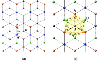
Figure 1: (a) Sketch of a dice lattice. (b) A hexagonal unit cell (yellow-shaded) of the lattice with NN and NNN hoppings. The black arrows $({\bf a}_{1},{\bf a}_{2}$ and ${\bf a}_{3})$ represent the NN hopping vectors of B-type atom while the orange dotted $({\bf b}_{1},{\bf b}_{2}$ and ${\bf b}_{3})$ and green dotted $(-{\bf b}_{1},-{\bf b}_{2}$ and $-{\bf b}_{3})$ arrows are the NNN hopping vectors for A-type and C-type atoms . In Haldane model, a flux distribution is considered which has the same periodicity as that of the lattice subject to the condition that total flux through every unit cell vanishes. A symmetric flux distribution is considered such that the triangular regions $a$ (or $b$) formed by the paths of NNN hoppings have identical flux passing through them.

The dice lattice can also be thought of as a limiting case of $\alpha$-$\mathcal{T}_{3}$ lattice Rizzi ; Raoux with $\alpha=1$. In recent years, there are several studies on diverse properties of the dice lattice such as orbital susceptibility Raoux , Klein tunneing Klein ; Klein1 , zero-momentum optical conductivity Illes ; Illes1 ; Cserti ; magneto-opt ; non-linear ; laser-opt , magnetotransport properties Tutul ; Malcolm ; duan ; Firoz , magnetoplasmons mag-plasmon , wave packet dynamics Tutul1 , electron states in the field of a charged impurity impurity ; impurity1 , role of Berry phase in photoinduced gap, topological phase transition under Floquet drivingat3floquet ; bdey , effect of electromagnetic radiation on dice lattice radiation ; radiation1 , electronic states of dice lattice ribbons dice-ribbon0 ; dice-ribbon ; dice-ribbon1 , Ruderman- Kittel-Kasuya-Yosida (RKKY) interaction RKKY and chaotic dynamics chaos .

The tight-binding Hamiltonian of dice lattice in the basis of sublattices A, B and C is given as

$$H_{0}(\textbf{k})=\frac{1}{\sqrt{2}}\left(\begin{array}[]{ccc}0&tf(\textbf{k})&0\\ tf^{*}(\textbf{k})&0&tf(\textbf{k})\\ 0&tf^{*}(\textbf{k})&0\end{array}\right),$$ (1)

where ${\bf k}=(k_{x},k_{y})$, $f(\textbf{k})=\sum_{j=1}^{3}\exp(-i{\bf k}\cdot{\bf a}_{j})$, ${\bf a}_{j}$ are the nearest neighbour (NN) vectors as shown in Fig. 1(b) and $t$ the NN hopping amplitudes. The explicit expressions of ${\bf a}_{j}$ are :– ${\bf a}_{1}=(\sqrt{3}/2,1/2)a_{0}$, ${\bf a}_{2}=(-\sqrt{3}/2,1/2)a_{0}$ and ${\bf a}_{3}=(0,1)a_{0}$ with $a_{0}$ being the lattice constant. The band structure comprises of a flat dispersionless band ($E_{0}=0$) flanked by two dispersive bands: $E_{\pm}=\pm t|f({\bf k})|$. The upper and lower bands are termed as conduction and valence bands respectively. The three bands touch each other with spin-1 Dirac-Weyl dispersion at two distinct points of the Brillouin zone ${\bf K}$ and ${\bf K}^{\prime}$ called Dirac points as shown in Fig. 2(a). The low energy excitations around these points are governed by a pseudospin-1 Dirac-Weyl Hamiltonian given by

$$H_{\mu}({\bf q})=\hbar v_{f}(\mu q_{x}S_{x}+q_{y}S_{y}).$$ (2)

Here, $S_{x}$ and $S_{y}$ are the usual spin-1 matrices, $v_{f}$ the Fermi velocity and ${\bf q}=(q_{x},q_{y})={\bf k-K}$ or ${\bf k-K^{\prime}}$. The index $\mu=+1$ and $-1$ represents ${\bf K}$ and ${\bf K}^{\prime}$ valleys respectively. Diagonalising the Hamiltonian (2), we get two linearly dispersive bands $E_{\pm}({\bf q})\equiv E_{\pm}(q)=\pm\hbar v_{f}q$ and the flat band $E_{0}=0$.

Exact flat band, massless low energy excitations and three-fold degeneracy at Dirac points are rather approximate for this lattice. The band structure does not retain these features when NNN hoppings are taken into account. The NNN hopping amplitudes for A-A and C-C sites are identical by symmetry (say $t_{2}$). The B-B NNN hopping vanishes since it encounters the high potential barrier between A and C atoms. When the NNN hoppings are included, the Hamiltonian takes the form

$$H(\textbf{k})=\frac{1}{\sqrt{2}}\left(\begin{array}[]{ccc}2\sqrt{2}\;t_{2}\;d({\bf k})&tf(\textbf{k})&0\\ tf^{*}(\textbf{k})&0&tf(\textbf{k})\\ 0&tf^{*}(\textbf{k})&2\sqrt{2}\;t_{2}\;d({\bf k})\end{array}\right),$$ (3)

where $d({\bf k})=\sum_{j=1}^{3}\exp(i{\bf k}\cdot{\bf b}_{j})$ where ${\bf b}_{j}$ are the NNN vectors as shown in Fig. 1(b) with ${\bf b}_{1}=(\sqrt{3},0)a_{0}$, ${\bf b}_{2}=(-\sqrt{3}/2,3/2)a_{0}$ and ${\bf b}_{3}=(-\sqrt{3}/2,-3/2)a_{0}$. Now, the bands are $E=2t_{2}\;d({\bf k})$ and $E_{\pm}=t_{2}\;d({\bf k})\pm\sqrt{t_{2}^{2}d^{2}({\bf k})+t^{2}|f({\bf k})|^{2}}$. Expanding $d({\bf k})$ around the Dirac point ${\bf K}$ gives

$$d({\bf q-K})=-\frac{3}{2}+\frac{9a_{0}^{2}q^{2}}{8}+\mathcal{O}(q^{3}).$$ (4)

At the Dirac point ${\bf K}$, the eigen values are $-3t_{2},-3t_{2}$ and $0$. This implies that a gap is created at the Dirac points reducing the three-fold degeneracy to two-fold, as shown in Fig. 2(b). The flat band also becomes dispersive. Although there is a band gap, the conduction band states near the Dirac points overlap with those of the distorted flat band near the ${\bf\Gamma}$ point of the Brillouin zone. This indirect overlap imparts metalic character to the system even if the flat band is completely filled. Moreover, the band touching between the distorted flat band and the valence band is quadratic in first order.

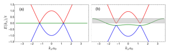
Figure 2: Tight-binding bands of dice lattice with (a) $t_{2}=0$ and (b) $t_{2}/t=0.06$. The gray shaded region shows the indirect overlap between the distorted flat band and the conduction band. The bands are plotted along the line joining the high-symmetry ${\bf K^{\prime},M}$ and ${\bf K}$ points.

Graphene with only NN hopping also hosts two gapless bands with massless quasiparticles at the Dirac points. The inclusion of next nearest neighbour (NNN) hopping adds a k-dependent scalar matrix to the tight-binding Hamiltonian in sublattice basis –

$$H_{t_{2}}^{g}(\textbf{k})=\left(\begin{array}[]{ccc}2t_{2}\;d({\bf k})&tf(\textbf{k})\\ tf^{*}(\textbf{k})&2t_{2}\;d({\bf k})\end{array}\right).$$ (5)

So, at any Dirac point, $E_{+}=E_{-}=2t_{2}\;d({\bf K})=-3t_{2}$. Thus, NNN hoppings only shift the Dirac points in graphene instead of opening up a gap goerbig .

III Haldane-like model of dice lattice

We consider a spatially periodic magnetic flux through the plane of the lattice such that total flux through the hexagonal unit cell centred around any hub site (B) vanishes, as shown in Fig. 1(b). Under such an orientation, the flux enclosed by hexagons formed by the paths of NN hoppings A-B or B-C also vanish by symmetry. Hence, the vector potential ${\bf A(r)}$ can be chosen to vanish along those paths so that NN hoppings do not acquire Aharonov-Bohm phases ($\sim\int^{NN}{\bf A(r)}\cdot d{\bf r}$). The flux enclosed by the triangle formed by NNN hoppings is non-zero. Hence, they aquire phases $\pm\phi_{h}\sim\pm\int^{NNN}{\bf A(r)}\cdot d{\bf r}$ such that $t_{2}\rightarrow t_{2}\mathrm{e}^{\pm i\phi_{h}}$. The sign of the phase is ‘$+$’ for clockwise and ‘$-$’ for counter-clockwise hopping. The value of $\phi_{h}$ is proportional to the flux enclosed by the three cyclic NNN hoppings A-A or C-C. On adding onsite energies $M$ (Semenoff mass) and $-M$ to A and C type atoms respectively, the lattice becomes a 3-level version of Haldane model. The Hamiltonian reads

$$\begin{aligned} H({\bf k})&=2t_{2}h_{0}({\bf k})\cos\phi_{h}S_{0}+(M-2t_{2}h_{z}({\bf k})\sin\phi_{h})S_{z}\\ &+t(g_{x}({\bf k})S_{x}+g_{y}({\bf k})S_{y}),\end{aligned}$$ (6)

where $g_{x}({\bf k})=\sum_{i=1}^{3}\cos({\bf k}\cdot{\bf a}_{i}),\;g_{y}({\bf k})=\sum_{i=1}^{3}\sin({\bf k}\cdot{\bf a}_{i}),\;h_{0}({\bf k})=\sum_{i=1}^{3}\cos({\bf k}\cdot{\bf b}_{i})$ and $h_{z}({\bf k})=\sum_{i=1}^{3}\sin({\bf k}\cdot{\bf b}_{i})$. Also, $S_{x},S_{y},S_{z}$ are the usual spin-1 matrices and $S_{0}\equiv$ diagonal matrix (1,0,1). The energy bands of Hamiltonian (6) are obtained in Appendix [A].

On choosing the hexagonal unit cell centred around a rim site (A or B) with the flux orientation identical to that in Fig. 1(b), the triangles formed by the NNN hoppings of the same rim site do not enclose any flux by symmetry. So, NNN hoppings of the corresponding rim site do not aquire any phase and may not be regarded as the conventional Haldane model.

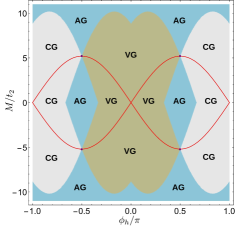
Figure 3: Phase diagram of Dice-Haldane model.

The phase diagram of the system governed by (6) is shown in Fig. 3. The region enclosed by the red curves represent topologically non-trivial phases while those outside it are trivial. The equations defining the red contours are $M=3\sqrt{3}\sin\phi_{h}$ and $M=-3\sqrt{3}\sin\phi_{h}$. The topological phase boundary is identical to that of Haldane model of graphene but there are several features which are in contrast. The topologically trivial and non-trivial phases are further divided into three categories – VG, CG and AG based on the band structure. The symbols VG, CG and AG stand for ‘valence-gapped’, ‘conduction-gapped’ and ‘all-gapped’ respectively. The ‘valence-gapped’ means that valence band is gapped while the distorted flat and conduction bands have indirect overlap with each other [Fig. 4(a)]. The overlap is similar to that in bare dice lattice with NNN hopping. The ‘conduction-gapped’ implies that conduction band is gapped while the other two have indirect overlap [Fig. 4(c)]. The ‘all-gapped’ indicates that all bands are well separated from each other having no overlap at all [Fig. 4(e)]. The red contour separates two VG (CG) phases because of closing and reopening of the band gap between the distorted flat and valence (conduction) bands along the contour [Fig. 4(b),(d)]. There are four independent purple points in the phase diagram at ($\pm 0.5,\pm 3\sqrt{3}$) where the conduction, flat and valence bands touch each other at either Dirac point with spin-1 Dirac-Weyl dispersion [Fig. 4(f)].

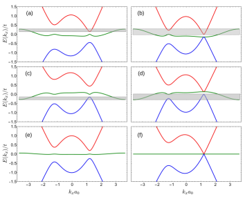
Figure 4: Band structure of different phases in Haldane model of dice lattice :– (a) A VG phase, (b) a phase on the contour separating two VG phases, (c) a CG phase, (d) a phase on the contour separating two CG phases, (e) an AG phase and (f) a semimetalic phase.

The Chern numbers of the conduction, (distorted) flat and valence bands in the topologically non-trivial AG phases around $\phi_{h}=\pm\pi/2$ are $\mp 2,0$ and $\pm 2$ respectively. In the non-trivial VG and CG phases for $\phi_{h}\lessgtr 0$, the Chern numbers of the gapped valence and conduction bands are $\mp 2$ and $\pm 2$ respectively. The Chern numbers have been calculated using the discretized Brillouin zone method proposed by Fukui et. al fukui . The system behaves as a Chern insulator when Fermi energy lies in a band gap of any of the of the topologically non-trivial phases. The system is metalic when Fermi energy lies in the range of overlapping bands in the topologically trivial as well as non-trivial VG and CG phases. The purple points can be termed as semimetalic when Fermi energy is at the three-fold band touching.

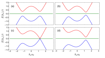
Figure 5: Band structure of Haldane-dice lattice for $t_{2}/t=0.06,\phi_{h}=\pi/2$ and :– (a) $M/t=0$, (b) $M/t=0.11$, (c) $M/t=0.31$ and (d) $M/t=0.51$.

For a particular choice of flux such that $\phi_{h}=\pi/2$, the Hamiltonian takes the form

$$\begin{aligned} H({\bf k})=(M-2t_{2}h_{z}({\bf k}))S_{z}+t(g_{x}({\bf k})S_{x}+g_{y}({\bf k})S_{y}).\end{aligned}$$ (7)

On diagonalizing, we get the bands $E_{0}=0$ and $E_{\pm}=\sqrt{t^{2}(g_{x}^{2}({\bf k})+g_{y}^{2}({\bf k}))+(M-2t_{2}h_{z}({\bf k}))^{2}}$. Here $E_{\pm}$ are two dispersive bands symmetrically gapped around a zero energy flat band $E_{0}$ as shown in Figs. 5(a)-(d)]. In this case, the flat band remains completely unperturbed by $t_{2}$. Thus, the flat band which becomes dispersive on inclusion of $t_{2}$ in bare dice lattice regains its flatness under the application of Haldane flux with $\phi_{h}=\pi/2$. In fact, a completely flat band occurs for $\phi_{h}=(2n+1)\pi/2$ where $n$ is an integer. Considering the symmetry in the band structure coming from pure imaginary NNN hoppings, we will consider the Haldane-dice model only with $\phi_{h}=\pi/2$ (and $M>0$) throughout the rest of the paper.

On linearizing the Hamiltonian (7) around the Dirac points ${\bf K}$ and ${\bf K}^{\prime}$, we get

$$H_{\mu}({\bf k})=\hbar v_{f}(\mu q_{x}S_{x}+q_{y}S_{y})+m_{\mu}v_{f}^{2}S_{z},$$ (8)

where $\mu$ represents valley index, ${\bf q}$ is a small momentum vector w.r.t a Dirac point, $v_{f}=3a_{0}t/2\hbar$ and $m_{\mu}v_{f}^{2}=(M-\mu\epsilon_{t_{2}})$ with $\epsilon_{t_{2}}=3\sqrt{3}t_{2}$. The Hamiltonian (8) is analogous to that of massive spin-1 Dirac quasiparticles in two dimensions. The low energy bands are $E_{0}({\bf q})=0$ and

$$E^{\mu}_{\pm}({\bf q})=\pm\sqrt{(\hbar v_{f}q)^{2}+(m_{\mu}v_{f}^{2})^{2}}.$$ (9)

The valley-symmetry of the band structure is not preserved due to breaking of TRS and inversion symmetry. The band gaps at ${\bf K}$ are smaller than at ${\bf K}^{\prime}$.

The z-component of Berry curvature of the bands around these points are

$$\Omega_{\pm}^{\mu}({{\bf q}})=\pm\mu\left[\frac{m_{\mu}\hbar^{2}v_{f}^{4}}{(\hbar^{2}v_{f}^{2}q^{2}+m_{\mu}^{2}v_{f}^{4})^{\frac{3}{2}}}\right],\hskip 14.22636pt\Omega_{0}^{\mu}({\bf q})=0.$$ (10)

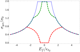
Figure 6: Variation of the Hall conductivity ($\sigma_{yx}$) with Fermi energy ($E_{f}$) for $\gamma=0$ (solid blue curve), $\gamma=1.6$ (lower, red dashed curve) and $\gamma=0.64$ (upper, green dashed curve).

The anomalous Hall conductivity is given byXiao-niu

$$\sigma_{yx}(E_{f})=\sigma_{0}\sum_{\lambda,\mu}\int_{0}^{\infty}\Omega_{\lambda}^{\mu}(q)f^{\mu}_{\lambda}(E_{f})qdq,$$ (11)

where $\lambda=0,\pm 1$, $\sigma_{0}=e^{2}/h$ and $f^{\mu}_{\lambda}(E_{f})=[\mathrm{e}^{(E_{\lambda}^{\mu}-E_{f})/k_{B}T}+1]^{-1}$ is the Fermi-Dirac distribution function. Using Eqs. (10) and (11), the Hall conductivity of the model at $T=0$ as a function of Fermi energy $E_{f}$ is obtained as –
Case I: $\gamma<1$

$$\frac{\sigma_{yx}(\epsilon_{f})}{\sigma_{0}}= \left(\frac{2}{|\epsilon_{f}|}\right)\theta[|\epsilon_{f}|-(\gamma+1)]+\left(1+\frac{1-\gamma}{|\epsilon_{f}|}\right)$$ (12)

$$\theta[|\epsilon_{f}|-|\gamma-1|]\theta[|\gamma+1|-|\epsilon_{f}|]+$$

$$\left(2\right)\theta[|\gamma-1|-|\epsilon_{f}|],$$

Case II: $\gamma>1$

$$\frac{\sigma_{yx}(\epsilon_{f})}{\sigma_{0}}= \left(\frac{2}{|\epsilon_{f}|}\right)\theta[|\epsilon_{f}|-(\gamma+1)]+\left(1+\frac{1-\gamma}{|\epsilon_{f}|}\right)$$ (13)

$$\theta[|\epsilon_{f}|-|\gamma-1|]\theta[|\gamma+1|-|\epsilon_{f}|],$$

Case III: $\gamma=0$

$$\frac{\sigma_{yx}(\epsilon_{f})}{\sigma_{0}}= \left(\frac{2}{|\epsilon_{f}|}\right)\theta[|\epsilon_{f}|-(\gamma+1)]+$$ (14)

$$\left(2\right)\theta[|\gamma-1|-|\epsilon_{f}|],$$

where $\epsilon_{f}=E_{f}/\epsilon_{t_{2}}$ and $\gamma=M/\epsilon_{t_{2}}$. The variation of Hall conductivity of the system with $E_{f}$ is shown in Fig. 6 for different values of $\gamma$. For $\gamma=0$, $\sigma_{yx}$ varies smoothly as $\sim 1/|E_{f}|$ when $E_{f}$ is below or above the band gap due to a valley-symmetric band structure. For $0<\gamma<1$ and $\gamma>1$, cusps appear in $\sigma_{yx}$ when $E_{f}$ enters or leaves the gap at ${\bf K}^{\prime}$ point due to asymmetry of band structure in the two valleys. For $\gamma<1$, the Chern number of valence and conduction bands are 2 and -2 respectively while that of flat band is zero. For $\gamma>1$, the Chern numbers of all the bands vanish and it acts like a trivial insulator. Thus, the Hall conductivity is quantized as $2\sigma_{0}$ and vanishes to 0 for $\gamma<1$ and $\gamma>1$ respectively when $E_{f}$ lies in the bulk band gap (at ${\bf K}$).

Dice lattice also hosts a Floquet topological phase identical to the case of Haldane model with $M=0$ and $\phi_{h}=\pi/2$, when shine with circularly polarized light bdey . A similar result was obtained for monolayer graphene where the commutator in the effective Floquet Hamiltonian in real space is equivalent to the second nearest neighbour hopping with phase $\pi/2$ of Haldane model kitagawa .

IV Edge states of Haldane-Dice nanoribbon

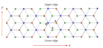
Figure 7: Schematic diagram of a dice nanoribbon with armchair edges.

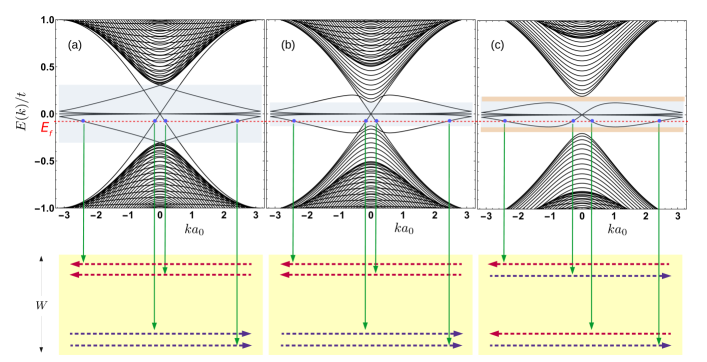
Figure 8: Low energy tight-binding bands of Haldane-dice nanoribbon for $\phi_{h}=\pi/2,\;t_{2}/t=0.06$ and (a) $\gamma=0$, (b) $\gamma=0.64$ and (c) $\gamma=1.6$, where $k=3k_{x}$. Schematic sketches of a part of the infinite nanoribbon are shown below the plots as yellow rectangles. The width $W$ of the nanoribbon = 41 hexagonal cells $\approx 71\;a_{0}$ . There are four edge states (blue dots) at the Fermi energy $E_{f}$ (dashed red line). For $\gamma<1$ i.e. the topologically non-trivial regime, there exists two chiral states at either edge [Figs. (a),(b)]. For $\gamma>1$ i.e. the topologically trivial case, the edge states are counter-propagating at either edge [Fig. (c)].

The calculation of the Chern number requires evaluation of Berry curvature $\Omega_{k_{x}k_{y}}$ and its integration over the 2D Brillouin zone. Hence, a two-component parameter space is mandatory for the concept of Chern number. However, mesoscopic measurements are done on narrow strips of a material. The finite width of the strip acts as a confining potential which breaks the periodicity of latttice along the confining direction and allows propagating states only in the direction perpendicular to it. The 2D bands of an insulator decompose into a set of densely spaced 1D sub-bands supriyo representing bulk states, with gaps in the spectra. For a Chern insulator, there exists a set of states in the gaps which connect two adjacent bulk bands. The wave functions of these states decay exponentially from the edge of the strip towards its bulk. They propagate along a fixed direction at either edge and hence are called chiral edge states. Due to their chiral nature, the edge states do not undergo backscattering from impurities and carry a dissipationless current. When the Fermi energy lies in a band gap, only the dissipationless edge states in the gap conduct, thereby giving rise to quantized Hall plateaus and nearly vanishing longitudinal resistance. The number of chiral edge states at the Fermi energy equals the sum of Chern numbers of all the 2D bulk bands below it. Thus, the bulk topological invariants manifest themselves as chiral edge states. This is called bulk-edge correspondence hatsugai .

We consider an armchair nanoribbon of the Haldane-dice lattice infinitely long along $x$ direction but having a finite width along $y$ as shown in Fig. 7. The tight-binding band structure of this strip is plotted for different values of $\gamma$ in Fig. 8. The blue dots represent the edge states at a given Fermi energy $E_{f}$ within the bulk band gap (shaded light blue). For $\gamma<1$, there are two chiral modes (unidirectional) confined at either edge at a given energy in the bulk gap, as shown in Figs. 8(a),(b). The velocities of the states at opposite edges are directed opposite to each other, thereby making them chiral. These states are responsible for quantized Hall conductance of $2e^{2}/h$ (neglecting spin) when $E_{f}$ lies in the bulk gap. This is consistent with Eq. (12) by bulk-edge correspondence. For $\gamma>1$, there exists no state within a particular range (orange shaded) of the bulk energy gaps, as shown in Fig. 8(c). So, the system will be a trivial insulator if $E_{f}$ lies in that range. However, there are counter-propagating edge states at either edge at energies close to flat band. These states exist even for $\gamma\gg 1$. This kind of edge states are absent in Haldane model of graphene in the non-topological regime which implies that they are peculiar to pseudospin-1 Dirac-Weyl system and arise because of the flat band. Due to counter propagation, the pair of edge states will not carry a net charge current at either edge and the system will behave as an insulator. Hence, bulk-boundary corresponds holds good in this case as well.

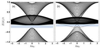
Figure 9: Tight-binding bands of the Haldane-dice nanoribbon in (a) topologically trivial [$\phi_{h}=0,M=2t_{2}$] and (b) topologically non-trivial [$\phi_{h}=0.25,M=2t_{2}$] VG phases.

The band structure of the nanoribbon in topologically trivial and non-trivial VG phases are shown in Fig. 9(a) and Fig. 9(b) respectively. In the trivial phase, no state exists in the bulk band gap (shaded light blue) while chiral edge states fill the bulk gap in the non-trivial regime. This testifies the topological nature of the system despite the ’metalic’ overlap between two bands. Similar edge states appear for non-trivial CG phases as well.

The armchair nanoribbon whose band structure is shown in Fig.(8) and (9) has number of atomic rows $N_{r}=83$ which is equal to $3N-1$ with $N=28$. It is known that the spectrum for an armchair nanoribbon is semimetalic for $N_{r}=3N-1$ and insulating otherwisedice-ribbon0 . It has been observed that in Haldane phases (with $\phi_{h}=\pi/2$), the spectra for $N_{r}=3N-1$ and $N_{r}\neq 3N-1$ are slightly different around the flat band, but the number and nature of edge states remain unaltered. The edge states for nanoribbons with zigzag boundaries have also been analyzed and similar results as armchair were obtained.

V Haldane model in quantizing magnetic field

Let the Haldane model be subjected to a uniform magnetic field ${\bf B}=B\hat{z}$. The vector potential ${\bf A}$ can be chosen in Landau gauge $(0,Bx,0)$ with $B>0$. We take the continuum model of massive Dirac Hamiltonian (8) near the Dirac points and incorporate the effect of magnetic field by minimal coupling ${\bf p}\rightarrow({\bf p}+e{\bf A})$. Then, the Hamiltonian can be written as

$$\hat{H}_{\mu}=v_{f}\left(\mu\hat{p}_{x}S_{x}+(\hat{p}_{y}+eB\hat{x})S_{y}\right)+m_{\mu}v_{f}^{2}S_{z}.$$ (15)

Since $[\hat{p}_{y},\hat{H}_{\mu}]=0$, an eigenstate can be chosen as $|\lambda_{\mu}(x)\rangle=\mathrm{e}^{iq_{y}y}|\psi_{\mu}(x)\rangle$, where $|\psi_{\mu}(x)\rangle=(a\phi_{a}^{\mu}(x)\hskip 8.5359ptb\phi_{b}^{\mu}(x)\hskip 8.5359ptc\phi_{c}^{\mu}(x))^{T}$. Substituting $|\lambda_{\mu}(x)\rangle$ in the Schrodinger equation, we get $H_{\mu}|\psi_{\mu}(x)\rangle=\epsilon_{\mu}|\psi_{\mu}(x)\rangle$ with

$$H_{\mu}=\left(\begin{array}[]{ccc}\epsilon_{m}&\epsilon_{B}f_{\mu}(\hat{x},\hat{p_{x}})&0\\ \epsilon_{B}f_{\mu}^{\dagger}(\hat{x},\hat{p_{x}})&0&\epsilon_{B}f_{\mu}(\hat{x},\hat{p_{x}})\\ 0&\epsilon_{B}f_{\mu}^{\dagger}(\hat{x},\hat{p_{x}})&-\epsilon_{m}\end{array}\right),$$ (16)

where $\epsilon_{m}^{\mu}=m_{\mu}v_{f}^{2}$, $\epsilon_{B}=v_{f}\sqrt{\hbar eB},f_{\mu}(\hat{x},\hat{p_{x}})=-i(\delta_{\mu,1}\hat{a}+\delta_{\mu,-1}\hat{a}^{\dagger})$. Here, $\hat{a}$ and $\hat{a}^{\dagger}$ are the lowering and raising operators of simple harmonic oscillator defined as

$$\hat{a}=\sqrt{\frac{eB}{2\hbar}}\left[\left(\hat{x}+\frac{\hbar q_{y}}{eB}\right)+i\frac{\hat{p}_{x}}{eB}\right]$$ (17)

and $\hat{a}^{\dagger}$ can be obtained by taking complex conjugate of $\hat{a}$. It turns out that the eigenspinor should be of the form

$$|\psi_{n}^{\mu}(x)\rangle=\left(\begin{array}[]{c}a_{n}^{\mu}\left(\delta_{\mu,1}u_{n-1}(x-X)+\delta_{\mu,-1}u_{n+1}(x-X)\right)\\ b_{n}^{\mu}u_{n}(x-X)\\ c_{n}^{\mu}\left(\delta_{\mu,1}u_{n+1}(x-X)+\delta_{\mu,-1}u_{n-1}(x-X)\right)\end{array}\right)$$ (18)

for $n\geq 1$, where $u_{n}(z)$ is eigenfunction of the $n$th level of harmonic oscillator and $X=-\hbar q_{y}/(eB)$. Using $\hat{a}u_{n}(x-X)=\sqrt{n}u_{n-1}(x-X)$ and $\hat{a}^{\dagger}u_{n}(x-X)=\sqrt{n+1}u_{n+1}(x-X)$ , we get the characteristic equation in eigenvalues $\epsilon$ as

$$\epsilon^{3}-\epsilon\left(\epsilon_{m}^{2}+(2n+1)\epsilon_{B}^{2}\right)+\mu\epsilon_{m}^{\mu}\epsilon_{B}^{2}=0.$$ (19)

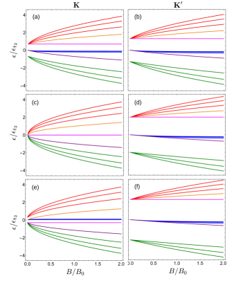
Figure 10: Variation of Landau level energies around ${\bf K}$ and ${\bf K^{\prime}}$ points with magnetic field for $\gamma=0.3$ [(a),(b)], $\gamma=1.0$ [(c),(d)] and $\gamma=1.3$ [(e),(f)].

Equation (19) has the form of a depressed cubic equation

$$\epsilon^{3}+\alpha\epsilon+\beta=0$$ (20)

. Its solutions are given by

$$\epsilon_{nj}^{\mu}=2\sqrt{\frac{-\alpha}{3}}\cos\Big{[}\frac{1}{3}\cos^{-1}\bigg{(}\frac{3\beta}{2\alpha}\sqrt{\frac{-3}{\alpha}}\bigg{)}-\frac{2\pi j}{3}\Big{]}$$ (21)

with $\alpha=-\left[(\epsilon_{m}^{\mu})^{2}+(2n+1)\epsilon_{B}^{2}\right]$, $\beta=\mu\epsilon_{m}^{\mu}\epsilon_{B}^{2}$ and $j=0,1$ and $2$. For $n\geq 1$, the eigenvalues or Landau level energies of each valley $\epsilon_{nj}^{\mu}$ are given by equation (21).

The components of the eigen spinors $\psi_{nj}^{\mu}$ are given by

$$a_{nj}^{\mu}=-i\left(\frac{\delta_{\mu,1}\sqrt{nB/B_{0}}+\delta_{\mu,-1}\sqrt{(n+1)B/B_{0}}}{\tilde{\epsilon}_{nj}^{\mu}-(\gamma-\mu)}\right)b_{nj}^{\mu},$$ (22)

$$c_{nj}^{\mu}=i\left(\frac{\delta_{\mu,1}\sqrt{(n+1)B/B_{0}}+\delta_{\mu,-1}\sqrt{nB/B_{0}}}{\tilde{\epsilon}_{nj}^{\mu}+(\gamma-\mu)}\right)b_{nj}^{\mu},$$ (23)

and

$$|b_{nj}^{\mu}| {}^{2}=\delta_{\mu,1}\left(1+\frac{nB/B_{0}}{(\tilde{\epsilon}_{nj}^{\mu}-(\gamma-\mu))^{2}}+\frac{(n+1)B/B_{0}}{(\tilde{\epsilon}_{nj}^{\mu}+(\gamma-\mu))^{2}}\right)$$ (24)

$$+\delta_{\mu,-1}\left(1+\frac{(n+1)B/B_{0}}{(\tilde{\epsilon}_{nj}^{\mu}-(\gamma-\mu))^{2}}+\frac{nB/B_{0}}{(\tilde{\epsilon}_{nj}^{\mu}+(\gamma-\mu))^{2}}\right),$$

where $\tilde{\epsilon}_{nj}^{\mu}=\epsilon_{nj}^{\mu}/\epsilon_{t_{2}}$ and $B_{0}=\epsilon_{t_{2}}^{2}/(e\hbar v_{f}^{2})$ is a magnetic field scale of the system.

Two other possible eigenspinors are $|\psi_{0}^{\mu}(x)\rangle=\left(\delta_{\mu,-1}a_{0}^{\mu}u_{1}(x-X)\hskip 8.5359ptb_{0}^{\mu}u_{0}(x-X)\hskip 8.5359pt\delta_{\mu,1}a_{0}^{\mu}u_{1}(x-X)\right)^{T}$ and $|\psi_{00}(x)\rangle=\left(\delta_{\mu,-1}u_{0}^{\mu}(x-X)\hskip 8.5359pt0\hskip 8.5359pt\delta_{\mu,1}u_{0}^{\mu}(x-X)\right)^{T}$ with energies $\epsilon_{0}^{\mu}=(-\mu\epsilon_{m}^{\mu}\pm\sqrt{(\epsilon_{m}^{\mu})^{2}+4\epsilon_{B}^{2}})/2$ and $\epsilon_{00}^{\mu}=-\mu\epsilon_{m}^{\mu}$ respectively. The amplitudes $a_{0}^{\mu}$ and $b_{0}^{\mu}$ are given by

$$a_{0}^{\mu}=\left(\frac{i\left(\delta_{\mu,1}-\delta_{\mu,-1}\right)\tilde{\epsilon}_{0}^{\mu}}{\sqrt{B/B_{0}}}\right)b_{0}^{\mu},\hskip 14.22636pt|b_{0}^{\mu}|=\left[1+\frac{(\tilde{\epsilon}_{0}^{\mu})^{2}}{B/B_{0}}\right]^{-1/2},$$ (25)

where $\tilde{\epsilon}_{0}^{\mu}=\epsilon_{0}^{\mu}/\epsilon_{t_{2}}$.

The variation of Landau level energies with magnetic field is shown in Fig. 10 for the two valleys. The valley-symmetry of the spectrum is broken for $\gamma\neq 0$. For no mass term (Semenoff or Haldane-like) in the Hamiltonian, we get infinite number of degenerate zero energy Landau levels Illes1 ; Tutul . The Haldane mass term splits all these levels shifting them towards positive or negative energy in each valley, as shown by blue curves in the figure. This was observed for massive dice lattice as well duan . In each valley, there exists a constant energy level $\epsilon_{00}^{\mu}$ denoted by pink lines, whose magnitude is equal to the magnitude of the mass term in the respective valleys. For $\gamma\neq 1$, the Landau levels in $K$ valley vary nearly as $\sim\sqrt{B}$ for $\epsilon_{m}\ll\epsilon_{B}$ [Figs. 10(a),(e)]. For $\gamma=1$, the energies scale exactly as $\sqrt{B}$ at $K$ valley [Fig. 10(c)], where the gap closes with massless spin-1 Dirac-Weyl dispersion. The mass term in the $K^{\prime}$ valley is large for $\gamma\geq 1$. In this case, the spectrum varies nearly as $\sim B$ for $\epsilon_{B}\ll\epsilon_{m}$ [Fig. 10(d),(f)].

VI Longitudinal conductivity

Using the Kubo formalism, the longitudinal conductivity $\sigma_{xx}$ is obtained as (see Appendix B for derivation)

$$\sigma_{xx}=\tilde{\sigma}_{0}\sum_{n,j,\mu}I_{nj}^{\mu}f_{nj}^{\mu}(\epsilon_{n,j}^{\mu})\left\{1-f_{nj}^{\mu}(\epsilon_{n,j}^{\mu})\right\},$$ (26)

where $\tilde{\sigma}_{0}=(g_{s}e^{2}n_{\rm im}V_{0}^{2})/(\pi h\Gamma_{0}k_{B}Tl_{0}^{2})$, $f_{nj}^{\mu}=(\mathrm{e}^{(\epsilon_{nj}^{\mu}-E_{f})/K_{B}T}+1)^{-1}$. Also, the term $I_{nj}^{\mu}$ is obtained as

$$I_{nj}^{\mu}= |a_{nj}^{\mu}|^{4}[\delta_{\mu,1}(2n-1)+\delta_{\mu,-1}(2n+3)]+|b_{nj}^{\mu}|^{4}(2n+1)$$ (27)

$$+|c_{nj}^{\mu}|^{4}[\delta_{\mu,1}(2n+3)+\delta_{\mu,-1}(2n-1)]-2|a_{nj}^{\mu}|^{2}|b_{nj}^{\mu}|^{2}$$

$$\times[\delta_{\mu,1}n+\delta_{\mu,-1}(n+1)]-2|b_{nj}^{\mu}|^{2}|c_{nj}^{\mu}|^{2}[\delta_{\mu,1}(n+1)$$

$$+\delta_{\mu,-1}n].$$

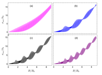
Figure 11: Longitudinal conductivity ($\sigma_{xx}$) of Haldane model of dice lattice as a function of inverse magnetic field ($1/B$) for (a) $\gamma=0$, (b) $\gamma=0.2$, (c) $\gamma=0.3$ and (d) $\gamma=0.4$. Other parameters are $E_{f}=4\epsilon_{t_{2}}$ and $k_{B}T=0.005\epsilon_{t_{2}}$.

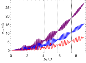
Figure 12: Longitudinal conductivity ($\sigma_{xx}$) of Haldane model of dice lattice as a function of inverse magnetic field ($1/B$) for $\epsilon_{f}=3.5$ (red), $\epsilon_{f}=4.5$ (blue) and $\epsilon_{f}=5.5$ (purple). Other parameters are $\gamma=0.3$ and $k_{B}T=0.005\epsilon_{t_{2}}$.

Substituting Eq. (27) into Eq. (26), we obtain the longitudinal conductivity as a function of $B$. In Fig. 11, $\sigma_{xx}/\tilde{\sigma}_{0}$ is plotted as a function of $B_{0}/B$ for different values of semenoff mass $M$ at a high $E_{f}$ in the conduction band. We get the usual SdH oscillations in $\sigma_{xx}$ for $M=0$. For finite $M$, beats appear in the SdH oscillations and the frequency of beats increases with $M$. In Fig. 12, the beating pattern is plotted for different values of $E_{f}$ for a given value of $M$. It is observed the number of oscillations between two nodes increases with $E_{f}$, but the beat frequency is apparently constant. Similar phenomena occurs when $E_{f}$ lies in the valence band.

To qualitatively explain the nature of the plots in Fig. 11,12, we consider an approximated formula of SdH oscillations in 2D electron system at low temperatures and low magnetic fields, which is given by sdh

$$\frac{\sigma_{xx}}{\sigma_{0}}=1-\lambda\sum_{\mu}\frac{2\pi^{2}k_{B}T/\epsilon_{B}}{\sinh(2\pi^{2}k_{B}T/\epsilon_{B})}\mathrm{e}^{-\frac{\pi\hbar}{\tau\epsilon_{B}}}\cos\left[\frac{\hbar S_{F}^{\mu}}{eB}+\phi_{0}^{\mu}\right],$$ (28)

where $\lambda$ is a constant, $\epsilon_{B}=\hbar\omega_{c}$, $\phi_{0}^{\mu}$ is the energy- and valley-dependent Berry phase and $S^{\mu}_{F}=\pi(k_{f}^{\mu})^{2}$ is the area enclosed by the Fermi circle in a given valley $\mu$. For massive dice lattice, $\phi_{0}^{\mu}=\mu(2\pi m_{\mu}v_{f}^{2}/E_{f})$. Using Eq. (9), we have $S_{F}^{\mu}=\pi\left(E_{f}^{2}-(m_{\mu}v_{f}^{2})^{2}\right)/(\hbar v_{f})^{2}$. The cosine terms of the two valleys act as harmonics with $S_{F}^{\mu}$ being the corresponding frequencies. The beats arise due to small difference in $S_{F}^{+}$ and $S_{F}^{-}$ due to difference in magnitude of mass terms in the two valleys. We can obtain the beat frequency by modelling the longitudinal concutivity as

$$\frac{\sigma_{xx}}{\sigma_{0}}\sim\cos\left(\frac{\hbar S_{F}^{+}}{eB}+\phi_{0}^{+}\right)+\cos\left(\frac{\hbar S_{F}^{-}}{eB}+\phi_{0}^{-}\right).$$ (29)

On simplification, we obtain

$$\frac{\sigma_{xx}}{\sigma_{0}}\sim\cos\left(2\pi\left[f_{m}\left(\frac{B_{0}}{B}\right)-\frac{1}{\epsilon_{f}}\right]\right)\cos\left(2\pi\gamma\left[\frac{B_{0}}{B}+\frac{1}{\epsilon_{f}}\right]\right),$$ (30)

where $\epsilon_{f}=E_{f}/\epsilon_{t_{2}}$ and $f_{m}=(\epsilon_{f}^{2}-\gamma^{2}-1)/2$ is the frequency of modulation. The second cosine factor in Eq. (30) gives the beating envelope with beat frequency $f_{b}=2\gamma$. The position of $j$-th beating node is $(B_{0}/B)_{j}=(2j-1)/4\gamma-1/\epsilon_{F}$ where $j=1,2,3...$ . The interval between two successive beating nodes is $\Delta=(B_{0}/B)_{j+1}-(B_{0}/B)_{j}=1/f_{b}$. The number of oscillations between two successive nodes is given by $N=f_{m}\Delta=(\epsilon_{F}^{2}-\gamma^{2}-1)/(4\gamma)$.

From Fig. 12, we have $(B_{0}/B)_{4}=5.72$ and $(B_{0}/B)_{5}=7.39$ which gives $\Delta_{plot}=1.67$. This exactly matches with the time period of beats given by $\Delta=1/(2\gamma)$. Also, in the SdH plot for $\epsilon_{f}=4.5$ in Fig. 12, we get nearly 16 oscillations between two successive nodes. This matches with the result $(=15.96)$ obtained from the expression for $N$.

The average frequency of oscillations arising from the two valleys is proportional to $E_{f}^{2}$. Thus, $N$ falls rapidly as $E_{f}$ approaches lower Landau levels of conduction or valence band and the beats gradually become indistinct. This is expected because the formation of beats requires the individual frequencies of the superposing harmonics to be much larger than their difference. So, well defined beats can be observed only when $E_{f}$ is large enough. In our analysis, we have chosen $E_{f}=4.5\epsilon_{t_{2}}$ which is close to $\sim 50^{th}$ Landau level of the conduction band at either valley for $\gamma=0.3$ and $B_{0}/B=5$. Similar beats are also expected for Haldane model of graphene.

It is to be noted that although the Landau levels are not valley-degenerate in massive dice lattice as well duan , it does not show beats in SdH oscillations.

VII Conclusion

We have constructed a theoretical Haldane-like model of dice lattice and investigated its topological properties within the tight-binding formalism. The phases of the system are dictated by the Semenoff mass, second neighbour hopping and periodic magnetic flux. Unlike the Haldane model of graphene which hosts phases representing a semi-metal, trivial insulator and a topogical insulator, this sytem supports a metalic phase in addition to the former. The metalic phase arises due to distortion of the flat band and its indirect overlap with either of the two other bands. These phases also gapped bands which may be topologically trivial or non-trivial. Chiral edge states show up in the band structure of a nanoribbon of the sytem in the non-trivial regime. A haldane phase with pure imaginary hoppings restores the dispersionless flat band. The Chern numbers of the bands are $-2,0$ and $2$ in the topological phases implying that the system may exhibit QAHE with two chiral edge channels. Exact expressions of Landau levels are derived from low-energy massive pseudospin-1 Dirac Hamiltonians around the two Dirac points. Peculiar beating pattern appears in the SdH oscillations of magneto-conductivity when the magnitude of mass terms in the two Dirac valleys are unequal and filling is close to the higher Landau levels of the conduction or valence band. The information about the phase-determining parameters of the system such as Semenoff mass, next neighbour hopping and Fermi energy can be extracted from the beat frequency and the number of oscillations between two successive beating nodes.

ACKNOWLEDGEMENTS

We would like to thank Sonu Verma and Ritajit Kundu for useful discussions.

Appendix A Energy bands of Haldane model

In this appendix, we present derivation of the energy bands of the Haldane model for dice lattice. The Hamitonian (6) yields the folowing characteristic equation of eigenvalues $\epsilon$ –

$$\epsilon^{3}-2p_{0}\epsilon^{2}-(p_{z}^{2}-p_{0}^{2}+2|p_{xy}|^{2})\epsilon+2p_{0}|p_{xy}|^{2}=0,$$ (31)

where $p_{0}=2t_{2}h_{0}({\bf k})\cos\phi_{h}$, $p_{z}=M-2t_{2}h_{z}({\bf k})\sin\phi_{h}$ and $p_{xy}=t\left(g_{x}({\bf k})-ig_{y}({\bf k})\right)/\sqrt{2}$. Solutions of this equation gives the band structure of the sytsem as functions of $M,t_{2}$ and $\phi_{h}$.

Equation (31) has the form

$$A\epsilon^{3}+B\epsilon^{2}+C\epsilon+D=0,$$ (32)

with $A=1,B=-2p_{0},C=-(p_{z}^{2}-p_{0}^{2}+2|p_{xy}|^{2})$ and $D=2p_{0}|p_{xy}|^{2}$. The solutions can be obtained by converting it to a depressed cubic equation. Substituting $\epsilon=\omega-B/3A$ in Eq. (32) and dividing by $A$, we get

$$\omega^{3}+p\omega+q=0,$$ (33)

where

$$p=\frac{3AC-B^{2}}{3A^{2}},\hskip 5.69046ptq=\frac{2B^{3}-9ABC+27A^{2}D}{27A^{3}}.$$ (34)

Equation (33) has the form of a depressed cubic equation with $p<0$ for all values of ${\bf k}$ in our system. Since all the eigenvalues are real, the solutions are of trigonometric form –

$$\omega_{j}=2\sqrt{\frac{-p}{3}}\cos\Big{[}\frac{1}{3}\cos^{-1}\bigg{(}\frac{3q}{2p}\sqrt{\frac{-3}{p}}\bigg{)}-\frac{2\pi j}{3}\Big{]},\hskip 5.69046ptj=0,1,2.$$ (35)

The energy bands of the Haldane model of the dice lattice are given by $\epsilon_{j}=\omega_{j}-B/3A$.

Appendix B Magnetoconductivity from the Kubo formula

Here we will provide the derivation of the analytical expression of the longitudinal conductivity in the linear response regime where the electric field is very weak. For this purpose we will be using the well-known Kubo formalism Kubo . In general, the longitudinal conductivity has diffusive and collisional contributions. In presence of quantizing magnetic field, the diffusive contribution exactly vanishes since the diagonal elements of the velocity operator are simply zero. Therefore, the longitudinal conductivity solely arises due to the collisional process.

In the framework of Kubo formalism, the general expression for the collisional conductivity in presence of quantizing magnetic field is given by vasilo ; Kubo_coll1 ; Kubo_coll3 ; Kubo_coll4

$$\sigma_{xx}=\frac{e^{2}}{Sk_{B}T}\sum_{\xi,\xi^{\prime}}f(\epsilon_{\xi})\{1-f(\epsilon_{\xi^{\prime}})\}W_{\xi\xi^{\prime}}(x_{\xi}-x_{\xi^{\prime}})^{2},$$ (36)

where $S$ is the surface area of the system, $\xi\equiv(j,n,q_{y},\mu)$ represents a set of all quantum numbers, $T$ being the temperature of the system, $x_{\xi}=\langle\xi|x|\xi\rangle=q_{y}l_{0}^{2}$, and $f(\epsilon_{\xi})=[\mathrm{e}^{(\epsilon_{\xi}-E_{f})/k_{B}T}+1]^{-1}$ is the Fermi-Dirac distribution function. Moreover, $W_{\xi\xi^{\prime}}$ describes the probability that an electron makes a transition from an initial state $|\xi\rangle$ to a final state $|\xi^{\prime}\rangle$. Its expression for elastic scattering by static impurities is given by

$$W_{\xi,\xi^{\prime}}=\frac{2\pi n_{\rm im}}{\hbar S}\sum_{\bf k}|V({\bf k})|^{2}|F_{\xi,\xi^{\prime}}|^{2}\delta(\epsilon_{\xi}-\epsilon_{\xi^{\prime}}),$$ (37)

where $n_{\rm im}$ is the impurity density and $V({\bf k})$ is the Fourier transform of the screened Coulomb potential $V({\bf r})=e^{2}\mathrm{e}^{-k_{s}r}/(4\pi\epsilon_{0}\epsilon_{r}r)$ with $\epsilon_{0}$ is the free space permittivity, $\epsilon$ is the dielectric constant of the medium and $k_{s}$ is the screened wave vector. The expression of $V({\bf k})$ for a 2D system is $V({\bf k})=e^{2}/(4\pi\epsilon_{0}\epsilon_{r}\sqrt{k^{2}+k_{s}^{2}})$. Finally, $F_{\xi,\xi^{\prime}}$ denotes the form factor which is defined as $F_{\xi,\xi^{\prime}}=\langle\xi^{\prime}|e^{i{\bf k}\cdot{\bf r}}|\xi\rangle$. We now consider only the intra-band ($j^{\prime}=j$) and intra-level ($n^{\prime}=n$) scattering because of the presence of the term $\delta(\epsilon_{\xi}-\epsilon_{\xi^{\prime}})$ in Eq. (37). The valley-dependent form factor is simplified as

$$|F_{nj}^{\mu}(u)|= [|a_{nj}^{\mu}|^{2}(\delta_{\mu,1}L_{n-1}(u)+\delta_{\mu,-1}L_{n+1}(u))$$ (38)

$$+|b_{nj}^{\mu}|^{2}L_{n}(u)+|c_{nj}^{\mu}|^{2}(\delta_{\mu,1}L_{n+1}(u)$$

$$+\delta_{\mu,-1}L_{n-1}(u))]\mathrm{e}^{-u/2},$$

where $L_{n}(u)$ is the Laguerre polynomial of order $n$.

The sharp Landau levels are broadened by the static impurities present in the system: $\delta(\epsilon_{\xi}-\epsilon_{\xi^{\prime}})=(1/\pi)\Gamma_{0}/[(\epsilon_{\xi}-\epsilon_{\xi^{\prime}})^{2}+\Gamma_{0}^{2}]$ with $\Gamma_{0}$ being the broadening parameter. It may be written as $\delta(\epsilon_{\xi}-\epsilon_{\xi^{\prime}})\simeq 1/(\pi\Gamma_{0})$ for intra-level and intra-band scattering. Further, $V({\bf k})$ is approximated as $V({\bf k})\simeq e^{2}/(4\pi\epsilon_{0}\epsilon k_{s})\equiv V_{0}$ since small values of $k^{2}$ will be contributing more due to the presence of exponentially decaying term $e^{-u}$ in the expressions of $\big{|}F_{n,j}^{\mu}\big{|}^{2}$.

Using the fact that $\sum_{q_{y}}\rightarrow g_{s}S/(2\pi l_{0}^{2})$ with $g_{s}$ being the spin-degeneracy and $\sum_{\bf k}\rightarrow S/(2\pi)^{2}\int k\,dk\,d\theta$ with $\theta$ being the polar angle of ${\bf k}$, we finally obtain the following expression for the longitudinal conductivity as

$$\sigma_{xx} = \tilde{\sigma}_{0}\sum_{j,\mu,n}I_{n,j}^{\mu}f\big{(}\epsilon_{n,j}^{\mu}\big{)}\left\{1-f\big{(}\epsilon_{n,j}^{\mu}\big{)}\right\},$$ (39)

where $\tilde{\sigma}_{0}=(g_{s}e^{2}n_{\rm im}V_{0}^{2})/(\pi h\Gamma_{0}k_{B}Tl_{0}^{2})$ and $I_{n,j}^{\mu}=\int_{0}^{\infty}u|F_{nj}^{\mu}(u)|^{2}\,du$. Using the standard results of $\int_{0}^{\infty}L_{n}^{2}(u)\mathrm{e}^{-u}udu=2n+1$ and $\int_{0}^{\infty}L_{n}(u)L_{n-1}(u)\mathrm{e}^{-u}udu=-n$, $I_{n,j}^{\mu}$ is obtained as

$$I_{n,j}^{\mu} =|a_{nj}^{\mu}|^{4}[\delta_{\mu,1}(2n-1)+\delta_{\mu,-1}(2n+3)]+|b_{nj}^{\mu}|^{4}(2n+1)$$

$$+|c_{nj}^{\mu}|^{4}[\delta_{\mu,1}(2n+3)+\delta_{\mu,-1}(2n-1)]-2|a_{nj}^{\mu}|^{2}|b_{nj}^{\mu}|^{2}$$

$$\times[\delta_{\mu,1}n+\delta_{\mu,-1}(n+1)]-2|b_{nj}^{\mu}|^{2}|c_{nj}^{\mu}|^{2}[\delta_{\mu,1}(n+1)$$

$$+\delta_{\mu,-1}n].$$

References

- (1) K. von Klitzing, Rev. Mod. Phys. 58, 519 (1986).
- (2) L. Saminadayar, D. C. Glattli, Y. Jin, and B. Etienne, Phys. Rev. Lett. 79, 2526 (1997).
- (3) R. B. Laughlin, Phys. Rev. B 23, 5632(R) (1981).
- (4) S. A. Trugman, Phys. Rev. B 27, 7539 (1983).
- (5) S. Ilani, J. Martin, E. Teitelbaum, J. H. Smet, D. Mahalu, V. Umansky, and A. Yacoby, Nature 427, 328 (2004).
- (6) P. Vasilopoulos, Phys. Rev. B 32, 771 (1985).
- (7) D. Tong, arXiv:1606.06687 (2016).
- (8) D. J. Thouless, M. Kohmoto, M. P. Nightingale, and M. den Nijs, Phys. Rev. Lett. 49, 405 (1982).
- (9) D. J. Thouless, Phys. Rev. B 27, 6083 (1983).
- (10) J. E. Avron, R. Seiler, and B. Simon, Phys. Rev. Lett. 51, 51 (1983).
- (11) M. Kohmoto, Ann. Phys. (Berlin) 160, 343 (1985).
- (12) Q. Niu, D. J. Thouless, and Yong-Shi Wu, Phys. Rev. B 31, 3372 (1985).
- (13) R. E. Prange, Girvin, M. Steven, Eds. (1990), The Quantum Hall effect (Springer-Verlag).
- (14) V. P. Gusynin, S. G. Sharapov, Phys. Rev. Lett. 95, 146801 (2005).
- (15) N. M. R. Peres, F. Guinea, A. H. C. Neto, Phys. Rev. B 73, 125411 (2006).
- (16) P. M. Krstajić and P. Vasilopoulos, Phys. Rev. B 83, 075427 (2012).
- (17) P. M. Krstajić and P. Vasilopoulos, Phys. Rev. B 86, 115432 (2012).
- (18) V. I. Fal′ko, Philos. Trans. Royal Soc. A 366, 205 (2007).
- (19) Kh. Shakouri, P. Vasilopoulos, V. Vargiamidis, and F. M. Peeters, Phys. Rev. B 90, 235423 (2014).
- (20) J L Lado and J Fernández-Rossier, 2D Mater. 3, 035023 (2016).
- (21) Y. Zhang, Y. Tan. H. Stormer, and P. Kim, Nature 438, 201–204 (2005).
- (22) Y. Jiang, Y. Zhang, Y. Tan. H. Stormer, and P. Kim, Science direct, Solid State Commun. 143, 14 (2007).
- (23) K. S. Novoselov, E. McCann, S. Morozov, V. I. Fal’ko, M. I. Katsnelson, U. Zeitler, D. Jiang, F. Schedin, and A. K. Geim, Nature Phys 2, 177–180 (2006).
- (24) L. Li, F. Yang, G. Ye, Z. Zhang, Z. Zhu, W. Lou, X. Zhou, L. Li, K. Watanabe, T. Taniguchi, K. Chang, Y. Wang, X. H. Chen, and Y. Zhang, Nature Nanotech 11, 593–597 (2016).
- (25) D. Bandurin, A. Tyurnina, and G. Yu, Nature Nanotech 12, 223–227 (2017).
- (26) N. Koirala, M. Salehi, J. Moon, and S. Oh, Phys. Rev. B 100, 085404.
- (27) F. D. M. Haldane, Phys. Rev. Lett. 61, 2015 (1988).
- (28) T. Kitagawa, T. Oka, A. Brataas, L. Fu, and E. Demler, Phys. Rev. B 84, 235108 (2011).
- (29) C. Liu, X. Qi, X. Dai, Z. Fang, and S-C. Zhang, Phys. Rev. Lett. 101, 146802 (2008)
- (30) Cui-Zu Chang, J. Zhang, X. Feng, J. Shen, Z. Zhang, and M. Guo, Science 340, 167–170 (2013).
- (31) J. W. Mclver, B. Schulte, F.-U. Stein, T. Matsuyama, G. Jotzu, G. Meier, and A. Cavalleri, Nat. Phys. 16, 38–41 (2020).
- (32) C. Chiu, J. C. Y. Teo, A. P. Schnyder, and S. Ryu, Rev. Mod. Phys. 88, 035005 (2016).
- (33) T. Andrijauskas, E. Anisimovas, M. Raciunas, A. Mekys, V. Kudriasov, I. B. Spielman, and G. Juzeliunas, Phys. Rev. A 92, 033617 (2015).
- (34) W. Liu, W. Lin, Z. D. Wang, and Y. Chen, Sci. Rep. 8, 12898 (2018).
- (35) B. Sutherland, Phys. Rev. B 34, 5208 (1986).
- (36) J. Vidal, R. Mosseri, and B. Doucot, Phys. Rev. Lett. 81, 5888 (1998).
- (37) S. E. Korshinov, Phys. Rev. B 63, 134503 (2001).
- (38) M. Rizzi, V. Cataudella, and R. Fazio, Phys. Rev. B 73, 144511 (2006).
- (39) D. Bercioux, D. F. Urban, H. Grabert, and W. Hausler, Phys. Rev. A 80, 063603 (2009).
- (40) J. D. Malcolm and E. J. Nicol, Phys. Rev. B 93, 165433 (2016).
- (41) M. Vigh, L. Oroszlány, S. Vajna, P. San-Jose, G. Dávid, J. Cserti, and Balázs Dora, Phys. Rev. B 88, 161413(R), (2013).
- (42) Yi-Xiang Wang, Fu-Xiang Li, and Ya-Min Wu, Euro. Phys. Lett. 105 17002 (2014).
- (43) R. Winkler, Spin-Orbit Coupling Effects in Two- Dimensional Electron and Hole Systems (Springer Verlag-2003).
- (44) F. Wang and Y. Ran, Phys. Rev. B 84, 241103 (2011).
- (45) A. Raoux, M. Morigi, J-N. Fuchs, F. Piechon, and G. Montambaux, Phys. Rev. Lett. 112, 026402 (2014).
- (46) D. F. Urban, D. Bercioux, M. Wimmer, and W. Haussler, Phys. Rev. B 84, 115136 (2011).
- (47) E. Illes and E. J. Nicol, Phys. Rev. B 95, 235432 (2017).
- (48) E. Illes, J. P. Carbotte, and E. J. Nicol, Phys. Rev. B 92, 245410 (2015).
- (49) E. Illes and E. J. Nicol, Phys. Rev. B 94, 125435 (2016).
- (50) A. D. Kovacs, G. David, B. Dora, and J. Cserti, Phys. Rev. B 95, 035414 (2017).
- (51) Y.-Ru Chen, Y. Xu, J. Wang, J-F. Liu, and Z. Ma, Phys. Rev. B 99, 045420 (2019).
- (52) L. Chen, J. Zuber, Z. Ma, and C. Zhang, Phys. Rev. B 100, 035440 (2019).
- (53) A. Iurov, L. Zhemchuzhna, D. Dahal, G. Gumbs, and D. Huang, Phys. Rev. B 101, 035129 (2020).
- (54) T. Biswas and T. K. Ghosh, J. Phys.: Condens. Matter 28, 495302 (2016).
- (55) J. D. Malcolm and E. J. Nicol, Phys. Rev. B 92, 035118 (2015).
- (56) SK Firoz Islam and P. Dutta, Phys. Rev. B 96, 045418 (2017).
- (57) Y. Xu and L.-M. Duan Phys. Rev. B 96, 155301 (2017).
- (58) A. Balassis, D. Dahal, G. Gumbs, A. Iurov, and D. Huang, arXiv:1905.04387.
- (59) T. Biswas and T. K. Ghosh, J. Phys.: Condens. Matter 30, 075301 (2018).
- (60) E. V. Gorbar, V. P. Gusynin, and D. O. Oriekhov, Phys. Rev. B 99, 155124 (2019).
- (61) D. Huang, A. Iurov, Hong-Ya Xu, Y-C. Lai, and G. Gumbs, Phys. Rev. B 99, 245412 (2019).
- (62) B. Dey and T. K. Ghosh, Phys. Rev. B 98, 075422 (2018).
- (63) B. Dey and T. K. Ghosh, Phys. Rev. B 99, 205429 (2019).
- (64) A. Iurov, G. Gumbs, and D. Huang, Phys. Rev. B 99, 205135 (2019).
- (65) M. A. Mojarro, V. G. Ibarra-Sierra, J. C. Sandoval-Santana, R. Carrillo-Bastos, G. G. Naumis, Phys. Rev. B 101, 165305 (2020).
- (66) D. O. Oriekhov, E. V. Gorbar and V. P. Gusynin, J. Low Temp. Phys. 44, 1313 (2018).
- (67) O. V. Bugaiko and D. O. Oriekhov, J. Phys.: Condens. Matter 31, 325501 (2019).
- (68) Mir W. Alam, B. Souayeh, and SK Firoz Islam, J. Phys.: Condens. Matter 31, 485303 (2019).
- (69) D. O. Oriekhov, and V. P. Gusynin, arXiv:2001.00272.
- (70) Chen-Di Han, Hong-Ya Xu, and Ying-Cheng Lai, Phys. Rev. Research 2, 013116 (2020).
- (71) M. O. Goerbig, Rev. Mod. Phys. 83, 1193 (2011).
- (72) T. Fukui, Y. Hatsugai, and H. Suzuki, J. Phys. Soc. Jpn. 74, 1674 (2005).
- (73) D. Xiao, M. Chang, and Q. Niu, Rev. Mod. Phys. 82, 1959 (2010).
- (74) S. Datta, Electronic Transport in Mesoscopic Systems, (Cambridge Univ. Press, Cambridge, 1995).
- (75) Y. Hatsugai, Phys. Rev. Lett. 71, 3697 (1993).
- (76) T. Ando, J. Phys. Soc. Jpn. 37, 1233 (1974); T. Ando, A. B. Bowler, and F. Stern, Rev. Mod. Phys. 54, 437 (1982).
- (77) G. M. Eliashberg, Sov. Phys.-JETP 14, 886 (1962).
- (78) M. Charbonneau, K. M. Van Vliet, and P. Vasilopoulos, J. Math. Phys. 23, 318 (1982).
- (79) F. M. Peeters and P. Vasilopoulos, Phys. Rev. B 46, 4667 (1992).
- (80) X. F. Wang and P. Vasilopoulos, Phys. Rev. B 67, 085313 (2003).