Accessible precisions for estimating two conjugate parameters using Gaussian probes

Abstract

We analyse the precision limits for simultaneous estimation of a pair of conjugate parameters in a displacement channel using Gaussian probes. Having a set of squeezed states as an initial resource, we compute the Holevo Cramér-Rao bound to investigate the best achievable estimation precisions if only passive linear operations are allowed to be performed on the resource prior to probing the channel. The analysis reveals the optimal measurement scheme and allows us to quantify the best precision for one parameter when the precision of the second conjugate parameter is fixed. To estimate the conjugate parameter pair with equal precision, our analysis shows that the optimal probe is obtained by combining two squeezed states with orthogonal squeezing quadratures on a 50:50 beam splitter. If different importance are attached to each parameter, then the optimal mixing ratio is no longer 50:50. Instead it follows a simple function of the available squeezing and the relative importance between the two parameters.

I Introduction

How precise can we make a set of physical measurements? This is a fundamental question that has driven much of the progress in science and technology. Improving the precisions and understanding limitations to measurements have often led to revolutionary discoveries or new insights in science. After overcoming technical sources of noise, the presence of quantum noise imposes a limit to the ultimate measurement precision. Due to the presence of quantum fluctuations, estimation precision using classical probe fields is limited to the standard quantum limit for optical measurements. In order to surpass this limit, quantum resource such as squeezed states Caves (1981); Xiao et al. (1987); Grangier et al. (1987) or entangled states D’Ariano et al. (2001); Fujiwara (2001); Fischer et al. (2001); Sasaki et al. (2002); Fujiwara and Imai (2003); Ballester (2004); Giovannetti et al. (2004); Genoni et al. (2013); Rigovacca et al. (2017); Bradshaw et al. (2017, 2018); Liu et al. (2018); Li et al. (2018); Gupta et al. (2018) are required. A notable example is the use of quadrature squeezed states of light to enhance the detection of gravitational wave Aasi et al. (2013); Grote et al. (2013). Another concept in quantum mechanics that distinguishes it from classical mechanics is that of non-commuting observables. This imposes a limitation for simultaneously estimating multiple parameters encoded in non-commuting observables.

In this work, we consider the problem of estimating two independent parameters $\theta=(\theta_{x},\theta_{y})$, encoded in two conjugate quadratures $X$ and $Y$ of a displacement channel $D(\theta)=\exp\left(\frac{i\theta_{y}}{2}X-\frac{i\theta_{x}}{2}Y\right)$. This channel induces a displacement of $\theta_{x}$ on the amplitude quadrature $X$ and $\theta_{y}$ on the phase quadrature $Y$ of a single-mode optical field with $[X,Y]=2i$. This problem has attracted a lot of attention since the early days of quantum mechanics Arthurs and Kelly (1965); Yuen (1982); Arthurs and Goodman (1988) and continue to do so Duivenvoorden et al. (2017); Genoni et al. (2013); Bradshaw et al. (2018). For example, if a single-mode probe is used to sense the displacement, the work by Arthurs and Kelly showed that the estimation mean squared errors $v_{x}$ and $v_{y}$ are bounded by $v_{x}v_{y}\geq 4$ Arthurs and Kelly (1965). However, it was theoretically shown Braunstein and Kimble (2000); Zhang and Peng (2000); Li et al. (2018) and experimentally demonstrated Li et al. (2002); Steinlechner et al. (2013); Liu et al. (2018) that by utilising quantum entanglement between two systems—for example through the quantum dense coding scheme—it is possible to circumvent this limit and estimate both parameters with accuracies beyond the standard quantum limit.

More recently, the pioneering works by Holevo and Helstrom on quantum estimation theory Helstrom (1967, 1969); Holevo (1976); *Holevo2011 have been used to study this problem Genoni et al. (2013); Gao and Lee (2014); Bradshaw et al. (2017, 2018). Once the probe state is specified, the quantum Fisher information determines a bound on the estimation precision thorough the quantum Cramér-Rao bound (CRB), which holds for every possible measurement strategy. There are many variants of the quantum CRB—the two most popular being the symmetric logarithmic derivative (SLD) Helstrom (1967, 1969); Braunstein and Caves (1994); Fujiwara and Nagaoka (1995) and the right logarithmic derivative (RLD) Yuen and Lax (1973); Belavkin (1976); Fujiwara (1994a, b); Fujiwara and Nagaoka (1995, 1999) as these yield direct bounds for the sum of the mean squared error. These have been widely used since they are relatively easy to compute Paris (2009); Petz and Ghinea (2011). For single-parameter estimation, the SLD-CRB offers an asymptotically tight bound on the precision Barndorff-Nielsen and Gill (2000). However for multi-parameter estimation, neither the SLD-CRB nor the RLD-CRB is necessarily tight Szczykulska et al. (2016); Suzuki (2019). Hence even though the probe might offer a large quantum Fisher information, their CRB might not be achievable, which means that the actual achievable precisions are not known.

Here, we solve this problem by using the Holevo Cramér-Rao bound to compute the actual asymptotically achievable precision Holevo (1976); *Holevo2011; Nagaoka (2005); Hayashi (2006); Yamagata et al. (2013). Knowing the achievable precision for a specific probe allows us to compare metrological performances between two different probes. We can then use this formalism to answer the question: Given a fixed quantum resource such as squeezing, how do we use it to optimally sense the channel? The resource states that we consider will be one-mode and two-mode Gaussian states, which we are allowed to freely mix or rotate before sending one mode to probe the channel. In doing so, we derive ultimate bounds on simultaneous parameter estimation which goes beyond existing restrictions imposed by the SLD or RLD-CRB. These bounds quantify a resource apportioning principle—the resource can be allocated to gain either a precise estimate of $\theta_{x}$ or $\theta_{y}$ but not both together Li et al. (2018); Liu et al. (2019).

The paper is organised as follows. We start with a summary of the general framework for two-parameter estimation in section II. Next we apply this framework to derive from the Fisher information precision limits for a single mode probe in section III. We then generalise this result to two-mode probes in section IV. We show that at least $6\text{\,}\mathrm{d}\mathrm{B}$ of squeezing is necessary to surpass the standard quantum limit. We also elucidate our results with two examples: the first with a single squeezed state and the second with two squeezed states with equal amount of squeezing. Finally, we end with some discussions in section V.

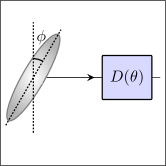
(a)

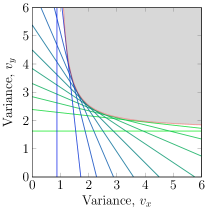
(b)

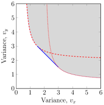
(c)

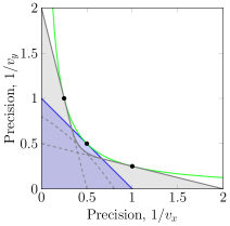
(d)

Figure 1: (a) A squeezed state is used to sense the parameter $\theta$ of a displacement channel. (b) With 3 dB of squeezing, and for a fixed squeezing angle $\phi=\pi/6$, each of the straight line is the Holevo-CRB (5) with a different value of $w_{x}/w_{y}$. The shaded area shows the accessible variance for simultaneously estimating $\theta_{x}$ and $\theta_{y}$. (c) The two red dashed and dotted lines can be achieved by an $X$ and $P$ squeezed state with $\phi=0$ and $\phi=\pi/2$ respectively. The blue line requires an intermediate squeezing angle. The shaded area are all the accessible regions for a single mode squeezed state. (d) This shows the same region as (c) but as a function of the precision. With a $3\text{\,}\mathrm{d}\mathrm{B}$ squeezed state, we can reach the grey areas. More squeezing can give a high precision for one parameter but at the expense of a lower precision for the other. The product of the precisions will never exceed $1/4$ regardless of the squeezing level. This is shown as the green line. The three grey dashed lines plot Eq. (8) when the squeezing angles are fixed at $\phi=0$, $\pi/4$ and $\pi/2$. The vacuum probe can only access the blue region.

II General framework

Let us begin with a brief review of the two-parameter estimation problem and the Holevo Cramér-Rao bound. To estimate the parameters $\theta$, the state $\rho_{0}$ is sent through the displacement channel $D(\theta)$ as a probe. After the interaction, the state becomes $\rho_{\theta}=D(\theta)\rho_{0}D(\theta)^{\dagger}$ which now contains information about the two parameters of interest. Next, we perform some measurement scheme and use an estimation strategy which leads to two unbiased estimators $\hat{\theta}_{x}$ and $\hat{\theta}_{y}$. We quantify the performance of these estimators, through the mean squared errors

$$v_{x}\coloneqq\mathbb{E}\left[(\hat{\theta}_{x}-\theta_{x})^{2}\right]\;\text{ and }\;v_{y}\coloneqq\mathbb{E}\left[(\hat{\theta}_{y}-\theta_{y})^{2}\right]\;.$$ (1)

When restricted to classical probes, due to quantum noise we have $v_{x}\geq 1$ and $v_{y}\geq 1$ which is known as the standard quantum limit. The aim of this work is to find out what are the possible values that $v_{x}$ and $v_{y}$ can take simultaneously. To quantify the performance for estimating both $\theta_{x}$ and $\theta_{y}$ simultaneously, we use the weighted sum of the mean squared error: $w_{x}v_{x}+w_{y}v_{y}$ as a figure of merit where $w_{x}$ and $w_{y}$ are positive weights that quantify the importance we attach to parameters $\theta_{x}$ and $\theta_{y}$ respectively. We want to find an estimation strategy that minimises this quantity.

The Holevo-CRB sets an asymptotically attainable bound on the weighted sum of the mean squared error Holevo (1976); *Holevo2011

$$w_{x}v_{x}+w_{y}v_{y}\geq f_{\text{HCR}}:=\min_{\mathcal{X}}h_{\theta}[\mathcal{X}]\;,$$ (2)

where $\mathcal{X}=\left\{\mathcal{X}_{x},\mathcal{X}_{y}\right\}$ are Hermitian operators that satisfy the locally unbiased conditions

$$\left.\text{tr}\left\{\rho_{\theta}\mathcal{X}_{j}\right\}\right\rvert_{\theta=0}=0\;\text{ and }\;\left.\text{tr}\left\{\frac{\partial\rho_{\theta}}{\partial\theta_{j}}\mathcal{X}_{k}\right\}\right\rvert_{\theta=0}=\delta_{jk}\;,$$ (3)

for $j,k\in\{x,y\}$ and $h_{\theta}$ is the function

$$h_{\theta}[\mathcal{X}]\coloneqq\text{Tr}\left\{W\,\text{Re}Z_{\theta}[\mathcal{X}]\right\}+\left\lVert\sqrt{W}\,\text{Im}Z_{\theta}[\mathcal{X}]\sqrt{W}\right\rVert_{1}\;.$$ (4)

Here $Z$ is the 2-by-2 matrix $Z_{jk}\coloneqq\text{tr}\left\{\rho_{\theta}\mathcal{X}_{j}\mathcal{X}_{k}\right\}$ and $W$ is a diagonal matrix with entries $w_{x}$ and $w_{y}$. The bound depends on the state $\rho_{\theta}$ only; it does not need for us to specify any measurement. For quadrature displacements with Gaussian probes, the bound involves minimisation of a convex function over a convex domain. This is an instance of convex optimisation problem which can be calculated efficiently by numerical methods Bradshaw et al. (2018). Furthermore, the optimisation also reveals an explicit measurement scheme that saturates the bound. For Gaussian probes, the optimal measurement will always be an individual Gaussian measurement.

III Precision bounds for single-mode probe

We now apply the formalism to a pure single-mode amplitude squeezed state probe with quadrature variance $e^{-2r}$ and rotated by an angle $\phi$ as shown in Fig. 1a. As previously stated, the Holevo-CRB only depends on the probe and how it varies with the parameters. In the single mode case, constraints (3) fully determines $f_{\text{HCR}}$. There is no free parameter in the optimisation and as a result, Holevo-CRB (2) becomes

$$w_{x}v_{x}+w_{y}v_{y}\geq w_{x}v_{a}+w_{y}v_{b}+2\sqrt{w_{x}w_{y}}\;,$$ (5)

where

$$v_{a} \coloneqq e^{-2r}\cos^{2}\phi+e^{2r}\sin^{2}\phi\;,$$ (6)

$$v_{b} \coloneqq e^{-2r}\sin^{2}\phi+e^{2r}\cos^{2}\phi\;,$$ (7)

are the projected variances on the $X$ and $Y$ quadratures. For every choice of $w_{x}/w_{y}$, Eq. (5) defines a straight line in the $v_{x}$–$v_{y}$ plane and gives a different bound on that plane. Some of these bounds are plotted in Fig. 1b for $e^{-2r}=1/2$ and $\phi=\pi/6$. For example, to estimate both $\theta_{x}$ and $\theta_{y}$ with equal precision, setting $w_{x}=w_{y}=1$ gives the best estimation strategy with $v_{x}+v_{y}=2(1+\cosh 2r)$ independent of $\phi$. This gets worse with more squeezing. However, if we are only concerned with estimating $\theta_{x}$, setting $w_{y}=0$ results in $v_{x}=v_{a}$. By eliminating $w_{x}$ and $w_{y}$ from Eq. (5), we can collect all these bounds into one stricter bound

$$(v_{y}-v_{b})(v_{x}-v_{a})\geq 1\;$$ (8)

which holds for every $\phi$. This is plotted in Fig. 1c for a few vales of $\phi$. Every pair of $(v_{x},v_{y})$ that satisfies Eq. (8) can be achieved by a specific measurement strategy. The same relation is plotted in Fig. 1d as a function of the precisions $1/v_{x}$ and $1/v_{y}$. This relation quantifies the resource apportioning principle—given a fixed amount of squeezing, there is only so much improvement in the precision to be had. The resource can be used to gain a precise estimate of $\theta_{x}$, but this comes at the expense of an imprecise estimate of $\theta_{y}$.

When $\phi=0$, relation (8) can be written concisely as a bound on the weighted sum of the precisions

$$\frac{e^{-2r}}{v_{x}}+\frac{e^{2r}}{v_{y}}\leq 1\;.$$ (9)

By using the arithmetic-geometric mean inequality, an immediate corollary of the result is the Arthurs and Kelly relation $v_{x}v_{y}\geq 4$ which holds for all $r$ Arthurs and Kelly (1965); Li et al. (2018). This reflects the Heisenberg uncertainty relation imposed on a single mode system. Every value of squeezing can saturate this inequality at one value of $v_{x}$ and $v_{y}$ as seen in Fig 1d. As we shall show next, this restriction can be somewhat relaxed using two mode states, but the sum of the precisions are still constrained by the total available resource.

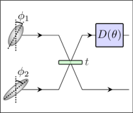
(a)

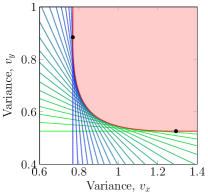
(b)

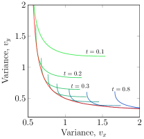
(c)

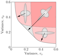
(d)

Figure 2: (a) Two squeezed states are used to sense the displacement $\theta$. (b) The Holevo-CR bound for a two-mode probe with $r_{1}=0.35$, $r_{2}=0.69$, $t=0.4$, $\phi_{1}=0$ and $\phi_{2}=\pi/2$. Each straight line correspond to a bound with different values of $w_{x}/w_{y}$. The pink region shows all the accessible values of $v_{x}$ and $v_{y}$. (c) Each bluish-green curve gives the accessible boundary for the same probe as (b) except for the value of $t$ which varies from $0.1$ to $0.8$ in steps of $0.1$. The red curve is the envelope of all the blueish-green curve. (d) The shaded areas show the relation (10) having two squeezed probes with $6\text{\,}\mathrm{d}\mathrm{B}$ and $15.6\text{\,}\mathrm{d}\mathrm{B}$ of squeezing. The variance for estimating both parameters can be simultaneously smaller than 1. The two grey dashed lines are limits when the probe is fixed with $\phi_{1}=0$ and $\pi/2$ given by Eq. (15).

IV Precision bounds for two-mode probe

We now consider a two-mode system where we have access to two amplitude-squeezed states with quadrature variances $e^{-2r_{1}}$ and $e^{-2r_{2}}$. Furthermore we are allowed to rotate them by $\phi_{1}$ and $\phi_{2}$, and mix the two through a beam-splitter of transmissivity $t$ before sending one mode through the displacement channel as shown in Fig. 2a. In this case, $f_{\text{HCR}}$ does not have a simple form; its computation involves finding the root of a quartic function. Despite this, the collection of all the bounds lead to a final expression that is surprisingly simple and intuitive. This is our main result: Given two pure squeezed states with variances $e^{-2r_{1}}$ and $e^{-2r_{2}}$ as a resource where $0\leq r_{1}\leq r_{2}$, and allowing for rotation and mixing operations, the measurement sensitivity is limited by

$$v_{y}\geq v_{y}^{*} =\left\{\begin{aligned} \frac{v_{x}e^{-2r_{1}}}{v_{x}-e^{-2r_{2}}}&\text{ if }&e^{-2r_{2}}\leq v_{x}<v_{c}\\ \left(e^{-r_{1}}+e^{-r_{2}}\right)^{2}-v_{x}&\text{ if }&v_{c}\leq v_{x}<v_{d}\\ \frac{v_{x}e^{-2r_{2}}}{v_{x}-e^{-2r_{1}}}&\text{ if }&v_{d}\leq v_{x}\end{aligned}\right.$$ (10)

where $v_{c}\coloneqq e^{-2r_{2}}+e^{-r_{1}-r_{2}}$ and $v_{d}\coloneqq e^{-2r_{1}}+e^{-r_{1}-r_{2}}$. The full derivation requires a lengthy but straightforward minimization and is relegated to the supplementary section. It involves finding the optimal values of $\phi_{1}$, $\phi_{2}$ and $t$ for every pair of $w_{x}$ and $w_{y}$. We outline the main steps in the derivations here. Firstly, for a fixed value of $w_{x}$ and $w_{y}$ and $t$, we can numerically compute the Holevo-CRB for each pair of $\phi_{1}$ and $\phi_{2}$. We find that the optimal setting for $\phi_{2}$ is when $\phi_{2}=\phi_{1}+\pi/2$, making the two squeezed states as different as possible Olivares and Paris (2011). Secondly, for a fixed $\phi_{1}$ and $t$, each pair of $w_{x}$ and $w_{y}$ gives a bound which correspond to one of the straight lines plotted in Fig 2b. The collection of all these bounds give the accessible region for this probe configuration. Thirdly, we vary $t$ to find the accessible region for a fixed $\phi_{1}$ as shown in Fig 2c. Finally the optimal value of $\phi_{1}$ is determined to arrive at the final result (10).

The region described by (10) is plotted in Fig. 2d. Every pair of $(v_{x},v_{y})$ that satisfies relation (10) can be attained by a dual homodyne measurement. An immediate corollary of this is the relation $v_{x}v_{y}\geq 4e^{-2r_{1}}e^{-2r_{2}}$ Steinlechner et al. (2013). In order to surpass the standard quantum limit for both parameters, we require $e^{-2r_{1}}e^{-2r_{2}}<{1}/{4}$. In other words, the sum of the squeezed variances of the resource has to be greater than approximately $6\text{\,}\mathrm{dB}$.

As mentioned in the outline of the derivations, not all regions in (10) can be reached using the same probe. Different region requires the resource to be used differently. For $w_{x}<w_{y}$, the best way to use the available resource is to set $\phi_{1}=0$ and $\phi_{2}=\pi/2$ and mix them on a beam-splitter with transmissivity

$$t=\frac{e^{r_{1}}}{e^{r_{1}}+e^{r_{2}}\sqrt{w_{x}/w_{y}}}\;.$$ (11)

This gives the optimal variances

$$v_{x} =e^{-2r_{1}}+e^{-(r_{1}+r_{2})}\sqrt{w_{y}/w_{x}}\;,$$ (12)

$$v_{y} =e^{-2r_{2}}+e^{-(r_{1}+r_{2})}\sqrt{w_{x}/w_{y}}\;,$$ (13)

or in terms of $t$,

$$v_{x}=\frac{e^{-2r_{1}}}{1-t}\;\text{ and }\;v_{y}=\frac{e^{-2r_{2}}}{t}$$ (14)

for $t>\frac{e^{r_{1}}}{e^{r_{1}}+e^{r_{2}}}$. After eliminating $t$, we arrive at a bound on the precisions

$$\frac{e^{-2r_{1}}}{v_{x}}+\frac{e^{-2r_{2}}}{v_{y}}\leq 1\;.$$ (15)

For $w_{y}<w_{x}$, we just need to swap the roles of $x$ and $y$ by setting $\phi_{1}=\pi/2$ and $\phi_{2}=0$. Equations (11)–(15) still hold with all $x$ and $y$ swapped. When $w_{x}=w_{y}$, there is a family of estimation strategy that all give the same sum of variances $v_{x}+v_{y}=(e^{-r_{1}}+e^{-r_{2}})^{2}$ but different values for each individual variances. This can be accessed by varying $\phi_{1}$ from $0$ to $\pi/2$ with $\phi_{2}=\phi_{1}+\pi/2$ and keeping $t$ as Eq. (11) which gives

$$\left.\begin{array}[]{c}v_{x}\\ v_{y}\end{array}\right\}=\frac{1}{2}\left(e^{-r_{1}}+e^{-r_{2}}\right)^{2}\pm\frac{\cos 2\phi_{1}}{2}\left(e^{-2r_{1}}-e^{-2r_{2}}\right)\;.$$ (18)

In the following, we illustrate these results with two examples. In these example, we present the optimal probe and measurement strategy that saturates the estimation precisions (10).

IV.1 Example 1: One squeezed state and one vacuum

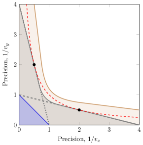
Figure 3: In order to surpass the standard quantum limit, $v_{x}v_{y}=1$ (red dashed line), we require access to an additional ancillary mode. The accessible region for a squeezed state with $6\text{\,}\mathrm{d}\mathrm{B}$ of squeezing is shown as the grey shaded region. It can just reach the standard quantum limit at the two black dots. The dashed and dotted grey lines plot Eqs. (20) and (22) which can be accessed by setting $\phi_{2}=\pi/2$ and $\phi_{2}=0$ respectively. With $9\text{\,}\mathrm{d}\mathrm{B}$ of squeezing, we can clearly surpass this limit (brown region). These bounds are given by Eq. (10).

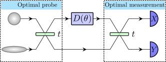
Figure 4: With one squeezed state and for $w_{x}<w_{y}$, the optimal probe configuration is to prepare a $Y$-squeezed and split it on a beam-splitter with $t=\frac{1}{1+\sqrt{w_{x}/w_{y}}}$. The optimal measurement is to disentangle the two modes on a second beam-splitter and perform $X$ and $Y$ quadrature measurements on the two outputs which gives the variances in (21).

In our first example, we consider the case of one squeezed state and one vacuum state ($r_{1}=0$) as shown in Fig. 3 inset.

For $w_{x}<w_{y}$, the optimal use of the probe is to set $\phi_{2}=\pi/2$ and the optimal measurement setup is shown in Fig. 4. The two quadrature measurements give independent estimates of $\theta_{x}$ and $\theta_{y}$ with variances

$$v_{x}=\frac{1}{1-t}\;\text{ and }\;v_{y}=\frac{e^{-2r_{2}}}{t}\;.$$ (19)

For $\frac{1}{1+e^{r_{2}}}\leq t\leq 1$, this pair of variances is optimal. Eliminating $t$, we can improve on the single mode precision relation (9) with

$$\frac{1}{v_{x}}+\frac{e^{-2r_{2}}}{v_{y}}\leq 1\;$$ (20)

which is plotted as the dashed grey line in Fig. 3 for $e^{-2r_{2}}=1/4$. For example, it is possible to have $v_{x}=2e^{-2r_{2}}$ and $v_{y}=2$ where the product $v_{x}v_{y}=4e^{-2r_{2}}$. If the resource variance $e^{-2r_{2}}<1/4$ (greater than $6\text{\,}\mathrm{dB}$), then $v_{x}v_{y}<1$, surpassing what is sometimes called the standard quantum limit.

For $w_{y}<w_{x}$, the optimal use of the probe is to set $\phi_{2}=0$ and the optimal measurement is similar to Fig. 4 but with the measurements $X$ and $Y$ swapped. Repeating as before, we get

$$v_{x}=\frac{e^{-2r_{2}}}{t}\;\text{ and }\;v_{y}=\frac{1}{1-t}$$ (21)

which is optimal when $\frac{1}{1+e^{r_{2}}}\leq t\leq 1$. In terms of the precisions, we have the relation

$$\frac{e^{-2r_{2}}}{v_{x}}+\frac{1}{v_{y}}\leq 1$$ (22)

which is plotted as the dotted grey line in Fig. 3 for $e^{-2r_{2}}=1/4$.

Finally to access the remaining region when $w_{x}=w_{y}$, we require $t=\frac{1}{1+e^{r_{2}}}$ and the squeezing angle $\phi_{2}$ to vary between $0$ and $\pi/2$. The optimal measurement is similar to Fig. 4 except that the quadrature measurement angles are set to $\phi_{2}+\pi/2$ in the upper arm and $\phi_{2}$ in the lower arm. Each of the measurement carry information on both $\theta_{x}$ and $\theta_{y}$. The two measurement outcomes, denoted by random variables $M_{1}$ and $M_{2}$, follow Gaussian distributions with

$$\text{mean}(M_{1}) =\sqrt{1-t}\left(\theta_{y}\cos\phi_{2}-\theta_{x}\sin\phi_{2}\right)\;,$$ (23)

$$\text{var}(M_{1}) =1\;,$$ (24)

and

$$\text{mean}(M_{2}) =\sqrt{t}\left(\theta_{y}\sin\phi_{2}+\theta_{x}\cos\phi_{2}\right)\;,$$ (25)

$$\text{var}(M_{2}) =e^{-2r_{2}}\;.$$ (26)

With this, we can form two unbiased estimators for $\theta_{x}$ and $\theta_{y}$:

$$\hat{\theta}_{x} =\frac{M_{2}\cos\phi_{2}}{\sqrt{t}}-\frac{M_{1}\sin\phi_{2}}{\sqrt{1-t}}\;,$$ (27)

$$\hat{\theta}_{y} =\frac{M_{2}\sin\phi_{2}}{\sqrt{t}}+\frac{M_{1}\cos\phi_{2}}{\sqrt{1-t}}\;.$$ (28)

The variances of these estimators are

$$\text{var}(\hat{\theta}_{x}) =\frac{e^{-2r_{2}}\cos^{2}\phi_{2}}{t}+\frac{\sin^{2}\phi_{2}}{1-t}$$ (29)

$$=\left(1+e^{r_{2}}\right)e^{-2r_{2}}\left(\cos^{2}\phi_{2}+e^{r_{2}}\sin^{2}\phi_{2}\right)\;,$$ (30)

and

$$\text{var}(\hat{\theta}_{y}) =\frac{e^{-2r_{2}}\sin^{2}\phi_{2}}{t}+\frac{\cos^{2}\phi_{2}}{1-t}$$ (31)

$$=\left(1+e^{r_{2}}\right)e^{-2r_{2}}\left(\sin^{2}\phi_{2}+e^{r_{2}}\cos^{2}\phi_{2}\right)\;,$$ (32)

which saturates the bound (18).

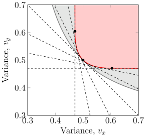
Figure 5: Precision limits with two $6\text{\,}\mathrm{d}\mathrm{B}$ squeezed resource. Each black dashed line is a Holevo-CRB (33) determined by a value of $w_{x}$ and $w_{y}$ for a specific probe where $t=0.5$. The Holevo-CRB is an attainable bound, which means that for each of this line, there is a measurement that can reach at least one point on it. The three dots corresponds to the three special cases discussed in the main text in Eq. (IV.2). The red line, which is the collection of all the black line bounds, gives the achievable variances for this probe. The grey shaded area, defined by Eq. (40) is the collection of all accessible regions we can attain by varying $t$. We see that the red region touches the grey line at only one point when $v_{x}=v_{y}$. To reach the other points on the grey line, we need to use the resource in a different way with $t\neq 0.5$.

IV.2 Example 2: Two equally squeezed state

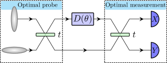
Figure 6: When $r_{1}=r_{2}$, for a fixed $w_{x}$ and $w_{y}$, the optimal probe that saturates the Holevo-CR bound is obtained by mixing the two squeezed states on a beam-splitter with $t$ set to $\frac{\sqrt{w_{y}}}{\sqrt{w_{x}}+\sqrt{w_{y}}}$. The optimal measurement is to disentangle the probe into a product of single-mode states and measure $X$ on the first mode and $Y$ on the second mode. This gives the variances in Eq. (39).

In our second example, we walk through the derivations of our main result in the special case where the initial resource are two squeezed states having an equal amount of squeezing $r_{1}=r_{2}=r$. In this case, when $\phi_{2}=\phi_{1}+\pi/2$, the Holevo-CRB can be simplified to

$$w_{x}v_{x}+w_{y}v_{y}\geq f_{\text{HCR}}=\min_{\lambda}\{w_{x}f_{x}+w_{y}f_{y}\}\;,$$ (33)

where

$$f_{x} \coloneqq\frac{\left(1+\lambda\sqrt{t}e^{r}\right)^{2}+\lambda^{2}(1-t)e^{-2r}}{\left(\lambda+\sqrt{t}e^{-r}\right)^{2}}\;,$$ (34)

$$f_{y} \coloneqq\frac{\left(1+\lambda\sqrt{t}e^{r}\right)^{2}+\lambda^{2}(1-t)e^{-2r}}{(1-t)e^{-2r}}\;.$$ (35)

In general, there is no analytical solution for the optimal value of $\lambda$. To see how this leads to the main result in Eq. (10), let us first consider a specific use of the resource by interfering the two squeezed states on a beam splitter with $t=0.5$ as shown in Fig. 2a. In this case, the optimal $\lambda$ that minimises $f_{\text{HCR}}$ is given by $\lambda^{*}={-}e^{-r}(1+\gamma)/\sqrt{2}$ where $\gamma$ is the positive solution to the quartic equation

$$\frac{w_{y}}{w_{x}}\gamma^{3}(\gamma-\tanh 2r)+\gamma\tanh 2r-1=0\;.$$ (36)

We can solve some special cases analytically:

$$(w_{x}=w_{y}=1) :\;v_{x}+v_{y}\geq 4e^{-2r} \text{ at }\lambda^{*} =-\sqrt{2}e^{-r}$$

$$(w_{x}=1,w_{y}=0) :\;v_{x}\geq\frac{1}{\cosh 2r} \text{ at }\lambda^{*} =\frac{-e^{r}}{\sqrt{2}\sinh 2r}$$

$$(w_{x}=0,w_{y}=1) :\;v_{y}\geq\frac{1}{\cosh 2r} \text{ at }\lambda^{*} =\frac{-e^{r}}{\sqrt{2}\cosh 2r}\,.$$ (37)

For other values of $w_{x}/w_{y}$, $\lambda^{*}$ can be calculated numerically and several of these bounds are plotted as the dashed lines in Fig. 5 when $e^{-2r}=1/4$. The envelope of these bounds is defined by the parametric equation $v_{x}=f_{x}$ and $v_{y}=f_{y}$ for ${-}\frac{e^{r}}{\sqrt{2}\sinh 2r}<\lambda<{-}\frac{e^{r}}{\sqrt{2}\cosh{2r}}$ and by construction can always be reached. This is the precision limit attainable by the probe and is plotted in red in Fig. 5. It is interesting to note that the optimal variance of $v_{x}=\frac{1}{\cosh 2r}$ can be achieved for any $v_{y}\geq\frac{\cosh 2r}{\sinh^{2}2r}$.

The optimal precision as given by Eq. (10) is plotted in grey in Fig. 5. We see that setting $t=0.5$ is only optimal when $w_{x}=w_{y}$ which gives $v_{x}=v_{y}=2e^{-2r}$ Steinlechner et al. (2013). For every other points on the grey line, a different probe configuration is needed to achieve it. In other words, assigning different weights to the precisions of the two quadratures will require the resource to be used differently. In the extreme case where we are interested in only one quadrature, the optimal scheme would be to just use one mode to sense the displacement, as in squeezed state interferometry Caves (1981); Xiao et al. (1987); Grangier et al. (1987). In general, when $w_{x}\neq w_{y}$, the optimal way to use the available resource is to mix the two squeezed states on an unbalanced beam-splitter with transmissivity $t^{*}=\frac{\sqrt{w_{y}}}{\sqrt{w_{x}}+\sqrt{w_{y}}}$. At this value of $t$, $f_{\text{HCR}}$ in Eq. (33) is minimised when $\lambda^{*}={-}{e^{-r}}/{\sqrt{t^{*}}}$ which gives Holevo-CRB as

$$f_{\text{HCR}}=\left(\sqrt{w_{x}}+\sqrt{w_{y}}\right)^{2}e^{-2r}\;.$$ (38)

The measurement that saturates this bound is shown in Fig. 6. After the second beam-splitter, the displaced two-mode probe is separated into two independent single-mode probes with displacements $\sqrt{1-t^{*}}\theta$ and $\sqrt{t^{*}}\theta$. Measuring $X$ on the first mode and $Y$ on the second gives

$$v_{x}=\frac{e^{-2r}}{1-t^{*}}\;\text{ and }\;v_{y}=\frac{e^{-2r}}{t^{*}}\;.$$ (39)

Upon eliminating $t^{*}$, we have

$$\frac{1}{v_{x}}+\frac{1}{v_{y}}=e^{2r}\;,$$ (40)

which saturates the bound (10). This precision relation quantifies the resource apportioning principle and implies that the quantum resource available through the squeezed states has to be shared between the two conjugate quadratures Liu et al. (2019). The effects of channel noise and inefficient detectors are presented in the supplementary materials.

V Discussions and conclusion

To summarise, we find precision bounds in simultaneous estimation of two conjugate quadratures. These bounds quantify a resource apportioning principle that limits how much precision is achievable with a given resource. While we restrict to pure states and two-mode states in this work to derive transparent analytical results, our formalism can be generalised to mixed and multi-mode Gaussian probes. These results can be applied to channel estimation when the amplitude and phase displacements have different strengths. For example, the phase signal can be much weaker than the amplitude signal we are trying to detect. This problem can also be formulated in a resource theory framework Idel et al. (2016); Takagi and Zhuang (2018); Albarelli et al. (2018); Yadin et al. (2018); Zhuang et al. (2018); Kwon et al. (2019), where squeezing is a resource and passive transformations are free operations. In this framework, the monotone that quantifies the value of the resource will depend on the weights $w_{x}$ and $w_{y}$ assigned to each parameter. What optimal means must depend on the application which assigns the weights $w_{x}$ and $w_{y}$.

References

- Caves (1981) Carlton M. Caves, “Quantum-mechanical noise in an interferometer,” Phys. Rev. D 23, 1693–1708 (1981).
- Xiao et al. (1987) Min Xiao, Ling-An Wu, and H. J. Kimble, “Precision measurement beyond the shot-noise limit,” Phys. Rev. Lett. 59, 278–281 (1987).
- Grangier et al. (1987) P. Grangier, R. E. Slusher, B. Yurke, and A. LaPorta, “Squeezed-light–enhanced polarization interferometer,” Phys. Rev. Lett. 59, 2153–2156 (1987).
- D’Ariano et al. (2001) G. Mauro D’Ariano, Paoloplacido Lo Presti, and Matteo G. A. Paris, “Using entanglement improves the precision of quantum measurements,” Phys. Rev. Lett. 87, 270404 (2001).
- Fujiwara (2001) Akio Fujiwara, “Quantum channel identification problem,” Phys. Rev. A 63, 042304 (2001).
- Fischer et al. (2001) Dietmar G. Fischer, Holger Mack, Markus A. Cirone, and Matthias Freyberger, “Enhanced estimation of a noisy quantum channel using entanglement,” Phys. Rev. A 64, 022309 (2001).
- Sasaki et al. (2002) Masahide Sasaki, Masashi Ban, and Stephen M. Barnett, “Optimal parameter estimation of a depolarizing channel,” Phys. Rev. A 66, 022308 (2002).
- Fujiwara and Imai (2003) Akio Fujiwara and Hiroshi Imai, “Quantum parameter estimation of a generalized pauli channel,” Journal of Physics A: Mathematical and General 36, 8093–8103 (2003).
- Ballester (2004) Manuel A. Ballester, “Estimation of unitary quantum operations,” Phys. Rev. A 69, 022303 (2004).
- Giovannetti et al. (2004) Vittorio Giovannetti, Seth Lloyd, and Lorenzo Maccone, “Quantum-enhanced measurements: beating the standard quantum limit,” Science 306, 1330 (2004).
- Genoni et al. (2013) MG Genoni, MGA Paris, G Adesso, H Nha, PL Knight, and MS Kim, “Optimal estimation of joint parameters in phase space,” Phys. Rev. A 87, 012107 (2013).
- Rigovacca et al. (2017) Luca Rigovacca, Alessandro Farace, Leonardo A. M. Souza, Antonella De Pasquale, Vittorio Giovannetti, and Gerardo Adesso, “Versatile gaussian probes for squeezing estimation,” Phys. Rev. A 95, 052331 (2017).
- Bradshaw et al. (2017) Mark Bradshaw, Syed M. Assad, and Ping Koy Lam, “A tight Cramér–Rao bound for joint parameter estimation with a pure two-mode squeezed probe,” Physics Letters A 381, 2598–2607 (2017).
- Bradshaw et al. (2018) Mark Bradshaw, Ping Koy Lam, and Syed M. Assad, “Ultimate precision of joint quadrature parameter estimation with a gaussian probe,” Phys. Rev. A 97, 012106 (2018).
- Liu et al. (2018) Yuhong Liu, Jiamin Li, Liang Cui, Nan Huo, Syed M. Assad, Xiaoying Li, and Z. Y. Ou, “Loss-tolerant quantum dense metrology with SU(1,1) interferometer,” Opt. Express 26, 27705 (2018).
- Li et al. (2018) Jiamin Li, Yuhong Liu, Liang Cui, Nan Huo, Syed M. Assad, Xiaoying Li, and Z. Y. Ou, “Joint measurement of multiple noncommuting parameters,” Phys. Rev. A 97, 052127 (2018).
- Gupta et al. (2018) Prasoon Gupta, Bonnie L. Schmittberger, Brian E. Anderson, Kevin M. Jones, and Paul D. Lett, “Optimized phase sensing in a truncated su(1,1) interferometer,” Opt. Express 26, 391 (2018).
- Aasi et al. (2013) J. Aasi, J. Abadie, B. P. Abbott, R. Abbott, T. D. Abbott, M. R. Abernathy, C. Adams, T. Adams, P. Addesso, R. X. Adhikari, and et al., “Enhanced sensitivity of the ligo gravitational wave detector by using squeezed states of light,” Nature Photonics 7, 613–619 (2013).
- Grote et al. (2013) H. Grote, K. Danzmann, K. L. Dooley, R. Schnabel, J. Slutsky, and H. Vahlbruch, “First long-term application of squeezed states of light in a gravitational-wave observatory,” Phys. Rev. Lett. 110, 181101 (2013).
- Arthurs and Kelly (1965) E. Arthurs and J. L. Kelly, “On the simultaneous measurement of a pair of conjugate observables,” Bell System Technical Journal 44, 725–729 (1965).
- Yuen (1982) Horace P. Yuen, “Generalized quantum measurements and approximate simultaneous measurements of noncommuting observables,” Physics Letters A 91, 101–104 (1982).
- Arthurs and Goodman (1988) E. Arthurs and M. S. Goodman, “Quantum correlations: A generalized heisenberg uncertainty relation,” Phys. Rev. Lett. 60, 2447–2449 (1988).
- Duivenvoorden et al. (2017) Kasper Duivenvoorden, Barbara M. Terhal, and Daniel Weigand, “Single-mode displacement sensor,” Phys. Rev. A 95, 2469–9934 (2017).
- Braunstein and Kimble (2000) Samuel L. Braunstein and H. J. Kimble, “Dense coding for continuous variables,” Phys. Rev. A 61, 042302 (2000).
- Zhang and Peng (2000) Jing Zhang and Kunchi Peng, “Quantum teleportation and dense coding by means of bright amplitude-squeezed light and direct measurement of a bell state,” Phys. Rev. A 62, 064302 (2000).
- Li et al. (2002) Xiaoying Li, Qing Pan, Jietai Jing, Jing Zhang, Changde Xie, and Kunchi Peng, “Quantum dense coding exploiting a bright einstein-podolsky-rosen beam,” Phys. Rev. Lett. 88, 047904 (2002).
- Steinlechner et al. (2013) Sebastian Steinlechner, Joran Bauchrowitz, Melanie Meinders, Helge Munro, W Jller-Ebhardt, Karsten Danzmann, and Roman Schnabel, “Quantum-dense metrology,” Nature Photonics 7, 626–630 (2013).
- Helstrom (1967) CW Helstrom, “Minimum mean-squared error of estimates in quantum statistics,” Phys. Lett. A 25, 101–102 (1967).
- Helstrom (1969) Carl W Helstrom, “Quantum detection and estimation theory,” Journal of Statistical Physics 1, 231–252 (1969).
- Holevo (1976) AS Holevo, “Noncommutative analogues of the Cramér-Rao inequality in the quantum measurement theory,” in Proceedings of the Third Japan—USSR Symposium on Probability Theory (Springer, 1976) p. 194–222.
- Holevo (2011) Alexander S Holevo, Probabilistic and statistical aspects of quantum theory, Vol. 1 (Springer Science & Business Media, 2011).
- Gao and Lee (2014) Yang Gao and Hwang Lee, “Bounds on quantum multiple-parameter estimation with gaussian state,” The European Physical Journal D 68, 1–7 (2014).
- Braunstein and Caves (1994) Samuel L. Braunstein and Carlton M. Caves, “Statistical distance and the geometry of quantum states,” Phys. Rev. Lett. 72, 3439–3443 (1994).
- Fujiwara and Nagaoka (1995) Akio Fujiwara and Hiroshi Nagaoka, “Quantum fisher metric and estimation for pure state models,” Phys. Lett. A 201, 119–124 (1995).
- Yuen and Lax (1973) H Yuen and Melvin Lax, “Multiple-parameter quantum estimation and measurement of nonselfadjoint observables,” IEEE Trans. Inform. Theory 19, 740–750 (1973).
- Belavkin (1976) Vyacheslav P Belavkin, “Generalized uncertainty relations and efficient measurements in quantum systems,” Theoretical and Mathematical Physics 26, 213–222 (1976).
- Fujiwara (1994a) Akio Fujiwara, “Multi-parameter pure state estimation based on the right logarithmic derivative,” Math. Eng. Tech. Rep 94, 94–10 (1994a).
- Fujiwara (1994b) Akio Fujiwara, “Linear random measurements of two non-commuting observables,” Math. Eng. Tech. Rep 94 (1994b).
- Fujiwara and Nagaoka (1999) Akio Fujiwara and Hiroshi Nagaoka, “An estimation theoretical characterization of coherent states,” J. Math. Phys. 40, 4227–4239 (1999).
- Paris (2009) Matteo GA Paris, “Quantum estimation for quantum technology,” Int. J. Quantum Inf. 7, 125–137 (2009).
- Petz and Ghinea (2011) D. Petz and C. Ghinea, “Introduction to quantum fisher information,” in Quantum Probability and Related Topics (World Scientific, 2011) Chap. 15, p. 261–281.
- Barndorff-Nielsen and Gill (2000) O E Barndorff-Nielsen and R D Gill, “Fisher information in quantum statistics,” J. Phys. A: Math. Gen. 33, 4481–4490 (2000).
- Szczykulska et al. (2016) Magdalena Szczykulska, Tillmann Baumgratz, and Animesh Datta, “Multi-parameter quantum metrology,” Advances in Physics: X 1, 621–639 (2016).
- Suzuki (2019) Jun Suzuki, “Information geometrical characterization of quantum statistical models in quantum estimation theory,” Entropy 21, 703 (2019).
- Nagaoka (2005) Hiroshi Nagaoka, “A new approach to Cramér-Rao bounds for quantum state estimation,” in Asymptotic Theory of Quantum Statistical Inference, edited by Masahito Hayashi (WORLD SCIENTIFIC, 2005) p. 100–112.
- Hayashi (2006) Masahito Hayashi, Quantum Information An Introduction (Springer Berlin Heidelberg, 2006).
- Yamagata et al. (2013) Koichi Yamagata, Akio Fujiwara, and Richard D. Gill, “Quantum local asymptotic normality based on a new quantum likelihood ratio,” The Annals of Statistics 41, 2197–2217 (2013).
- Liu et al. (2019) Yuhong Liu, Nan Huo, Jiamin Li, Liang Cui, Xiaoying Li, and Zheyu Jeff Ou, “Optimum quantum resource distribution for phase measurement and quantum information tapping in a dual-beam SU(1,1) interferometer,” Opt. Express 27, 11292 (2019).
- Olivares and Paris (2011) Stefano Olivares and Matteo G. A. Paris, “Fidelity matters: The birth of entanglement in the mixing of gaussian states,” Phys. Rev. Lett. 107, 170505 (2011).
- Idel et al. (2016) Martin Idel, Daniel Lercher, and Michael M Wolf, “An operational measure for squeezing,” Journal of Physics A: Mathematical and Theoretical 49, 445304 (2016).
- Takagi and Zhuang (2018) Ryuji Takagi and Quntao Zhuang, “Convex resource theory of non-gaussianity,” Phys. Rev. A 97, 062337 (2018).
- Albarelli et al. (2018) Francesco Albarelli, Marco G. Genoni, Matteo G. A. Paris, and Alessandro Ferraro, “Resource theory of quantum non-gaussianity and wigner negativity,” Phys. Rev. A 98, 052350 (2018).
- Yadin et al. (2018) Benjamin Yadin, Felix C. Binder, Jayne Thompson, Varun Narasimhachar, Mile Gu, and M. S. Kim, “Operational resource theory of continuous-variable nonclassicality,” Phys. Rev. X 8, 041038 (2018).
- Zhuang et al. (2018) Quntao Zhuang, Peter W. Shor, and Jeffrey H. Shapiro, “Resource theory of non-gaussian operations,” Phys. Rev. A 97, 052317 (2018).
- Kwon et al. (2019) Hyukjoon Kwon, Kok Chuan Tan, Tyler Volkoff, and Hyunseok Jeong, “Nonclassicality as a quantifiable resource for quantum metrology,” Phys. Rev. Lett. 122, 040503 (2019).