Field-induced transitions of the Kitaev material $\alpha$-RuCl₃ probed by thermal expansion and magnetostriction

Abstract

High-resolution thermal expansion and magnetostriction measurements were performed on single crystals of $\alpha$-RuCl₃ in magnetic fields applied parallel to the Ru-Ru bonds. The length changes were measured in the direction perpendicular to the honeycomb planes. Our data show clear thermodynamic characteristics for the field-induced phase transition at the critical field $\mu_{\mathrm{0}}H_{\mathrm{c}1}=7.8(2)$ T where the antiferromagnetic zigzag order is suppressed. At higher fields, a kink in the magnetostriction coefficient signals an additional transition or crossover around $\mu_{\mathrm{0}}H_{\mathrm{c}2}\approx 11$ T. The extracted Grüneisen ratio shows typical hallmarks for quantum criticality near $H_{\mathrm{c}1}$, but also displays anomalous behavior above $H_{\mathrm{c}1}$. We compare our experimental data with spin-wave calculations employing a minimal Kitaev-Heisenberg model in the semiclassical limit. Most of the salient features are in agreement with each other, however, the peculiar features in the region above $H_{\mathrm{c}1}$ cannot be accounted for in our semiclassical modelling and hence suggest a genuine quantum nature. We construct a phase diagram for $\alpha$-RuCl₃ in a magnetic field along the Ru-Ru bonds, displaying a zigzag ordered state below $H_{\mathrm{c}1}$, a quantum paramagnetic regime between $H_{\mathrm{c}1}$ and $H_{\mathrm{c}2}$, and a semiclassical partially polarized state above $H_{\mathrm{c}2}$.

I Introduction

The search for realizations of topological quantum spin liquids (QSLs) has generated a tremendous excitement, for both fundamental reasons and potential applications, e.g., in quantum information processing Nayak et al. (2008). QSLs are characterized by long-range entanglement, topological order and associated ground-state degeneracies, as well as fractionalized quasiparticles. Kitaev’s spin-1/2 model on the honeycomb lattice Kitaev (2006) is a paradigmatic example for a QSL because it uniquely combines exact solvability in terms of Majorana fermions and experimental relevance Jackeli and Khaliullin (2009); Chaloupka et al. (2010); Trebst ; Banerjee et al. (2017).

One of the prime candidates to realize Kitaev magnetism is the compound $\alpha$-RuCl₃: It is a $J_{\rm eff}$ = 1/2 Mott insulator with a layered structure of edge-sharing RuCl₆ octahedra arranged in a honeycomb lattice Plumb et al. (2014); Sears et al. (2015); Johnson et al. (2015); Majumder et al. (2015); Kubota et al. (2015); Sinn et al. (2016); Ziatdinov et al. (2016); Weber et al. (2016). While $\alpha$-RuCl₃ displays magnetic long-range order of so-called zigzag type, a moderate in-plane magnetic field suppresses the magnetic order, resulting in a paramagnetic state whose nature has been debated Yadav et al. (2016); Leahy et al. (2017); Kasahara et al. (2018). By now, the existence of a quantum spin-liquid regime in $\alpha$-RuCl₃ in a window of applied magnetic field is suggested by a number of experimental results, such as an excitation continuum in neutron scattering Do et al. (2017); Banerjee et al. (2018); Balz et al. (2019), in Raman scattering Sandilands et al. (2015), as well as in microwave/terahertz absorption measurements Wang et al. (2017); Wellm et al. (2018), and, most prominently, an approximately half-quantized thermal Hall conductivity Kasahara et al. (2018); Yokoi et al. . The latter has been associated with the presence of a chiral Majorana edge mode, characteristic of a Kitaev spin liquid in applied magnetic field Cookmeyer and Moore (2018); Vinkler-Aviv and Rosch (2018). Theoretically, a field-induced spin liquid has been discussed for microscopic models relevant to $\alpha$-RuCl₃ Jiang et al. (2019); Gordon et al. (2019); Kaib et al. (2019).

However, the structure of the field-temperature phase diagram of $\alpha$-RuCl₃ is not settled: The experiments of Refs. Kasahara et al., 2018; Balz et al., 2019; Yokoi et al., suggest the existence of at least three low-temperature phases, i.e., a spin-liquid phase sandwiched between the zigzag and high-field phases. Yet clear-cut thermodynamic evidence for a transition between the spin-liquid and high-field phase is lacking, perhaps with the exception of a signature in the magnetocaloric effect Balz et al. (2019). Moreover, the spin-liquid signatures have not been traced to very low temperatures, hence they may as well represent a quantum critical regime instead of a stable phase.

In this paper, we report a thorough dilatometric study of $\alpha$-RuCl₃ in in-plane magnetic fields up to $14$ T and temperatures down to $2.4$ K. Thermal expansion (TE) and magnetostriction (MS) represent thermodynamic properties governed by magnetoelastic coupling, enabling us to study the nature of the different phase transitions and possible critical behavior. We confirm the field-induced suppression of long-range order at a critical field of $\mu_{\mathrm{0}}H_{\mathrm{c}1}=7.8(2)$ T and provide strong thermodynamic evidence for quantum critical behavior at $H_{\mathrm{c}1}$ by analyzing the Grüneisen ratio. This is confirmed by our MS data, which moreover displays signatures of an additional weak first-order transition or crossover around $\mu_{\mathrm{0}}H_{\mathrm{c}2}\approx 11$ T. A comparison of our experimental data to semiclassical calculations in a minimal spin model yields qualitative agreement for many features, but also hints at additional physics between $H_{\mathrm{c}1}$ and $H_{\mathrm{c}2}$ beyond semiclassics. On basis of our experimental data we conjecture a field-temperature phase diagram of $\alpha$-RuCl₃ for in-plane fields along the Ru-Ru bonds containing three distinct low-temperature regimes.

II Experiments

II.1 Methods

High-quality single crystals of $\alpha$-RuCl₃ with a thickness of $\sim 1$ mm were grown using a vapor-transport technique Banerjee et al. (2017). Via angular-dependent magnetization measurments Janssen et al. (2017); Lampen-Kelley et al. (2018) the sample was properly aligned to ensure that the magnetic field was applied parallel to the Ru-Ru bond direction. This is the field direction where the additional ordered phase found in Ref. Lampen-Kelley et al., is absent or very narrow.

The linear TE and MS of $\alpha$-RuCl₃ were determined by using a custom-built capacitive dilatometer with a parallel-plate system consisting of two separately aligned capacitor plates, which detect changes of the uniaxial sample length $\Delta L_{i}$. The sample is clamped between one of the plates and the frame of the dilatometer, and thus is exposed to a small force via the springs of the dilatometer. Note that this force in combination with the van-der-Waals bonds between the honeycomb planes of $\alpha$-RuCl₃ leads to an irreversible mechanical deformation of the sample along $ab$. Thus, all TE and MS studies were performed for the configuration $\Delta\vec{L}\parallel c^{*}$, $\Delta\vec{L}\perp\vec{H}$ for this van-der-Waals bonded material, with $c^{*}$ being perpendicular to the crystallographic $ab$ plane. For the TE the temperature $T$ was swept from 3 K to 300 K using sweep rates between 0.03 K/min and 0.2 K/min. The MS was measured at constant temperatures between 2.4 K and 10 K and slowly sweeping the magnetic fields from 0 T to 14 T (sweep rates of 0.01 T/min and 0.03 T/min). A correction for the TE of the dilatometer itself has been applied using high-purity Cu reference samples. Measurements were performed on two different single crystals with a thickness of $\sim 1.0$ mm (sample #1) and $\sim 0.8$ mm (sample #2).

Specific-heat measurements under applied magnetic fields $\vec{H}\parallel$ Ru-Ru bonds up to $14$ T were performed on the same single crystal used for the dilatometry measurements (sample #1). For the experiments a heat-pulse relaxation method was used in a Physical Property Measurement System (PPMS, Quantum Design). In order to obtain the intrinsic specific heat of $\alpha$-RuCl₃, the temperature- and field-dependent addenda were subtracted from the measured specific-heat values in the sample measurements. In order to estimate the phononic contribution, the specific heat of the non-magnetic structural analog compound RhCl₃ in polycrystalline form was measured Wolter et al. (2017).

II.2 Thermal expansion

In Fig. 1 the normalized linear TE measured along the $c^{*}$ direction,

$$\frac{\Delta L_{c^{*}}(T,\mu_{0}H)}{L_{c^{*}}(300\,\text{K},0\,\text{T})}\equiv\frac{L_{c^{*}}(T,\mu_{0}H)-L_{c^{*}}(T_{\rm ref},0\,{\rm T})}{L_{c^{*}}(300\,\text{K},0\,\text{T})},$$ (1)

of $\alpha$-RuCl₃ is depicted for zero field as well as for some representative in-plane magnetic fields $\vec{H}\parallel$ Ru-Ru bonds. $\Delta L_{c^{*}}$ is the measured length change along the $c^{*}$ direction, which is then normalized to the sample length at room temperature. $T_{\rm ref}=3.6$ K represents a minimum reference temperature at which $L_{c^{*}}$ was measured for every data set and thus our data refer to, i.e., the TE is zero at $T_{\rm ref}$ and vanishing field.

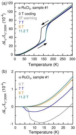
Figure 1: Normalized linear TE of $\alpha$-RuCl₃ perpendicular to the $ab$ plane, $\Delta L_{c^{*}}/L_{c^{*},300\,\text{K}}$, as function of temperature for both zero and finite applied magnetic fields $\vec{H}\parallel$ Ru-Ru bonds; (a) full temperature interval up to $300$ K, (b) low-temperature region up to $30$ K.

The zero-field $c^{*}$-axis TE is rather large, as expected for weakly bonded van-der-Waals materials, Fig. 1(a). Further, the overall TE is decreasing upon lowering temperature, which is in line with an overall shrinking of the lattice constants compared to room temperature Johnson et al. (2015); Park et al. . Interestingly, a step-like feature is seen in our TE data at around $T_{\mathrm{s,c}}\approx 137$ K upon cooling, clearly indicating a first-order structural transition. The transition is strongly hysteretic, with $T_{\mathrm{s,w}}\approx 161$ K upon warming. It likely corresponds to a change from a high-temperature monoclinic $C2/m$ structure to a low-temperature rhombohedral $R\bar{3}$ structure Park et al. . Note that $T_{\mathrm{s,c}}$ and thus also the hysteresis upon this transition strongly depend on the used temperature sweep rate.

Looking at the details at low temperatures in zero field, Fig. 1(b), the overall shrinking of the $c^{*}$-axis TE is followed by a broad minimum at $\sim 14$ K and a subsequent expansion of the $c^{*}$ axis down to lowest temperatures. Furthermore, a sharp kink is clearly discernable at the antiferromagnetic transition temperature $T_{\mathrm{N}}=7.2(1)$ K. While the TE for $T\gtrsim$ 100 K is not particularly sensitive to the application of an in-plane magnetic field, the low-temperature TE changes dramatically up to the critical field $\mu_{\mathrm{0}}H_{\mathrm{c}1}=7.8(2)$ T at which the kink signalling the antiferromagnetic transition is finally completely suppressed. For fields larger than $H_{\mathrm{c}1}$ a positive TE is discernable.

Overall, our TE data are in good agreement with x-ray diffraction and former zero-field TE experiments Park et al. ; He et al. (2018), showing a rearrangement of the unit cell of $\alpha$-RuCl₃ both at the structural and the antiferromagnetic phase transitions, and thus also a coupling of the lattice and spin degrees of freedom in our compound.

In order to better resolve the magnetic phase transitions, we also analyze the linear TE coefficient along the $c^{*}$ direction,

$$\alpha_{c^{*}}=\frac{\partial}{\partial T}\frac{\Delta L_{c^{*}}(T,\mu_{0}H)}{L_{c^{*}}(300\,\text{K},0\,\text{T})}$$ (2)

Anomalies in $\alpha_{c^{*}}(T)$ typically correspond to phase transitions. Low-temperature results for $\alpha$-RuCl₃ are shown in Fig. 2(a). At zero field the sharp peak signifies a single phase transition at $T_{\mathrm{N}}=7.2(1)$ K. With increasing field the peak broadens, reduces in magnitude, and shifts to lower temperatures, until it disappears at $\mu_{0}H_{\mathrm{c}1}=7.8(2)$ T. Given the agreement with other probes, we conclude that this peak represents the magnetic transition into the zigzag phase. It highlights that the low-$T$ contributions to $\alpha_{c^{*}}$ are primarily magnetic, and also underlines the quality of our single crystals, with a dominant ABC stacking of the hexagonal layers along $c^{*}$.

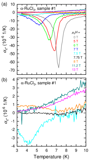
Figure 2: The linear TE coefficient perpendicular to the $ab$ plane, $\alpha_{c^{*}}$, of $\alpha$-RuCl₃ for zero and applied magnetic fields $\vec{H}\parallel$ Ru-Ru bonds. (a) General overview of $\alpha_{c^{*}}$ with the focus on the ordered antiferromagnetic zigzag transition and its shift as function of the applied field. (b) A zoom of the data for applied fields close to the critical field $\mu_{\mathrm{0}}H_{\mathrm{c}1}$ = 7.8(2) T.

Fig. 2(b) displays a magnified region of Fig. 2(a) for fields near and above $H_{\mathrm{c}1}$. The low-$T$ linear TE shows a sign change close to the critical field $H_{\mathrm{c}1}$; at $H_{\mathrm{c}1}$ the TE coefficient is tiny up to about $8$ K, indicating that the phonon contribution is small in this temperature regime. For fields of $11.2$ T and $13$ T, $\alpha_{c^{*}}(T)$ is positive and monotonic. In this high-field regime, the magnitude of $\alpha_{c^{*}}$ decreases with increasing field, consistent with an increasing magnetic excitation gap in the polarized high-field phase as observed by various methods, such as nuclear magnetic resonance and thermal conductivity Baek et al. (2017); Hentrich et al. (2018). Interestingly, the data at $8$ T are anomalous in that $\alpha_{c^{*}}$ shows a non-monotonic $T$ dependence, suggesting the existence of a distinct intermediate-field region between the zigzag and high-field phases, as recently also observed with other techniques Kasahara et al. (2018); Yokoi et al. ; Balz et al. (2019).

II.3 Grüneisen ratio

The linear TE coefficient is proportional to the derivative of the entropy with respect to uniaxial pressure along the $c^{*}$ axis, $\partial S/\partial p_{c^{*}}$, as discussed in detail below (see Sec. III.1). Therefore, vanishing $\alpha_{c^{*}}$ near $H_{\mathrm{c}1}$ indicates a maximum of the magnetic contribution to the entropy, $S_{\rm mag}$, at the critical field. In fact, such an entropy accumulation is predicted to occur near a continuous quantum phase transition Zhu et al. (2003); Garst and Rosch (2005), and can be identified experimentally by measuring the Grüneisen ratio, commonly defined as the ratio between the magnetic contributions to the volume TE coefficient and the specific heat $C_{p,\mathrm{mag}}$,

$$\Gamma=V_{\mathrm{m}}\frac{\alpha_{\rm mag}}{C_{p,\rm mag}}=-\frac{(\partial S_{\rm mag}/\partial p)_{T}}{T(\partial S_{\rm mag}/\partial T)_{p}},$$ (3)

where $V_{\mathrm{m}}\simeq 55.9\,\text{cm}^{3}/\text{mol}$ is the molar volume Johnson et al. (2015); Park et al. ; Cao et al. (2016). $\Gamma$ displays characteristic divergencies Zhu et al. (2003) upon approaching a pressure-driven quantum critical point (QCP), and both $\Gamma$ and $\alpha_{\rm mag}$ change sign near a QCP as a result of entropy accumulation in the quantum critical regime Garst and Rosch (2005).

Upon applying this concept to $\alpha$-RuCl₃ two remarks are in order: (i) Its phase transition(s) can be driven by both field and pressure, therefore both the field and pressure derivatives of the entropy will display sign changes, making $\Gamma$ a suitable probe to detect QCPs. (ii) For the qualitative analysis, we use the linear $c^{*}$-axis (instead of volume) TE coefficient $\alpha_{c^{*}}$, which is much larger compared to that along the other directions He et al. (2018).

To calculate the Grüneisen ratio, the specific heat of $\alpha$-RuCl₃ is needed. The corresponding specific-heat coefficient $C_{p}/T$ is shown in Fig. 3 as a function of temperature and magnetic field $\vec{H}\parallel$ Ru-Ru bonds. The data agree with previous reports for unknown in-plane field directions Wolter et al. (2017); Widmann et al. (2019), with a single magnetic transition at zero field at $T_{N}=7.1(1)$ K defined at the peak position of $C_{p}/T$. For $\mu_{\mathrm{0}}H\gtrsim 8$ T the peak and thus the magnetic long-range order disappears, as expected.

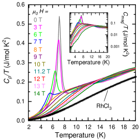
Figure 3: Specific-heat coefficient $C_{p}/T$ of $\alpha$-RuCl₃ as function of temperature for applied magnetic fields $\vec{H}\parallel$ Ru-Ru bonds, together with $C_{p}/T$ data for nonmagnetic RhCl₃ (black stars). The inset shows the magnetic contribution $C_{p,\rm mag}/T$ of $\alpha$-RuCl₃ on a semi-logarithmic scale.

For both $\alpha_{c^{*}}$ and $C_{p}$ the phononic contribution is assumed to be field-independent and had to be determined and subtracted from the $\alpha$-RuCl₃ data. The phononic contribution to the specific heat of $\alpha$-RuCl₃ was approximated by the specific heat of the non-magnetic structural analog compound RhCl₃ (see Fig. 3), after scaling its experimental specific heat curve by the Lindemann factor Lindemann (1910), which was found to be 1.000059. For the phononic contribution of $\alpha_{c^{*}}(T)$ we used the $\alpha$-RuCl₃ data at $7.75$ T as an approximation. Alternative schemes are discussed in Appendix B.

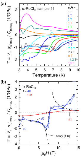
Figure 4: The Grüneisen ratio $\Gamma$ of $\alpha$-RuCl₃ in a magnetic field along the Ru-Ru bonds. (a) $\Gamma(T)$ for different fields up to 13 T. (b) $\Gamma(H)$ for $4$ K and $10$ K and for two different samples (#1, #2). The dash-dotted line shows the theoretical calculation for $\Gamma$ at $4$ K whose overall amplitude has been scaled to match the low-field part of the data. Close to $H_{\mathrm{c}1}$ no results are shown as the spin-wave approximation becomes unreliable, see text.

The resulting Grüneisen ratio $\Gamma$ is depicted in Figs. 4(a) and 4(b) as function of temperature and applied magnetic field $\vec{H}\parallel$ Ru-Ru bonds, respectively. A more comprehensive data set, including measurements of different samples, is shown in Appendix A. As function of field, $\Gamma$ changes sign at $H_{\mathrm{c}1}$ as expected. For fields below $H_{\mathrm{c}1}$, $\Gamma(T)$ displays a peak at the Néel temperature $T_{\rm N}(H)$, while becoming small at high $T$, Fig. 4(a). Moreover, below $H_{\mathrm{c}1}$ and at low $T$, $\Gamma(H)$ has its largest magnitude close to $H_{\mathrm{c}1}$, Fig. 4(b). The low-field part thus appears consistent with quantum critical phenomenology Garst and Rosch (2005), and the fact that $\Gamma(T)$ does not change sign at a temperature $T\gtrsim T_{\mathrm{N}}$ (Fig. 4(a)) implies a large fluctuation regime above the quasi-two-dimensional magnetic transition. Together, the data signifies a continuous quantum phase transition at $H_{\mathrm{c}1}$ – the same conclusion was reached earlier based on a detailed analysis of low-T specific-heat measurements Wolter et al. (2017).

The low-$T$ data for $\Gamma$ above $H_{\mathrm{c}1}$ are again anomalous, in that there is no appreciable field dependence in $\Gamma(H)$ between $8$ and $11$ T. As a result, the behavior of $\Gamma(H)$ around $H_{\mathrm{c}1}$ is rather asymmetric, Fig. 4(b). We note that $\Gamma$ for fields of $13$ T and above displays large error bars at low $T$ because both $\alpha_{c^{*},\rm mag}$ and $C_{p,\rm mag}$ become very small as the magnetic excitations are gapped out.

II.4 Magnetostriction

Field-driven phase transitions can be efficiently studied in MS experiments, measuring the length change as function of the applied field at constant $T$. Results for the linear MS coefficient along $c^{*}$,

$$\lambda_{c^{*}}=\frac{\partial}{\partial(\mu_{0}H)}\frac{\Delta L_{c^{*}}(T,\mu_{0}H)}{L_{c^{*}}(300\,{\rm K},0\,{\rm T})},$$ (4)

are displayed in Fig. 5. At $T=2.4$ K the continuous transition at $H_{\mathrm{c}1}$ causes a sharp peak in $\lambda_{c^{*}}$ at $\mu_{0}H=7.8(2)$ T, which broadens and shifts to lower fields upon increasing temperature, thus tracking $T_{\mathrm{N}}(H)$. At $10$ K (i.e., above $T_{\mathrm{N}}$), $\lambda_{c^{*}}$ deviates from a linear field dependence that would be expected for a usual paramagnet. This is again related to the large fluctuation regime reaching up to temperatures of the exchange couplings ($\sim 50$ K); we recall that $\alpha$-RuCl₃ has been characterized as a “Kitaev paramagnet” in this regime Do et al. (2017); Jansa et al. (2018).

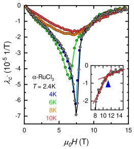
Figure 5: The linear MS coefficient $\lambda_{c^{*}}$ as function of field and different temperatures (sample 1). The inset highlights the kink observed in $\lambda_{c^{*}}$ at 2.4 K.

A striking feature is seen in the low-$T$ MS data above $H_{\mathrm{c}1}$: While the 2.4 K data of $\lambda_{c^{*}}(H)$ show no signature for a second continuous transition, the curve displays a clear kink at $\mu_{0}H_{\mathrm{c}2}\approx 11$ T, see inset of Fig. 5. Upon increasing the temperature, the kink position varies only weakly while the kink magnitude (i.e. the change in slope) decreases, with the kink disappearing for temperatures above $8$ K. These observations suggest the existence of an additional low-temperature quantum regime whose field width remains finite at the lowest temperatures and should therefore be distinguished from the narrow quantum critical regime near $H_{\mathrm{c1}}$ and the semiclassical partially polarized regime above $H_{\mathrm{c2}}$.

III Theory

III.1 Methods

III.1.1 $J_{1}$-$K_{1}$-$\Gamma_{1}$-$J_{3}$ model

For a theoretical description of the thermodynamic behavior of $\alpha$-RuCl₃, we employ a minimal spin model containing nearest-neighbor Heisenberg $J_{1}$, Kitaev $K_{1}$, and off-diagonal $\Gamma_{1}$ interaction, as well as a third-nearest-neighbor Heisenberg $J_{3}$ interaction on the two-dimensional honeycomb lattice Winter et al. (2016),

$$\mathcal{H} =\sum_{\langle ij\rangle}\left[J_{1}\vec{S}_{i}\cdot\vec{S}_{j}+K_{1}S_{i}^{\gamma}S_{j}^{\gamma}+\Gamma_{1}(S_{i}^{\alpha}S_{j}^{\beta}+S_{i}^{\beta}S_{j}^{\alpha})\right]$$

$$\quad+\sum_{\langle\!\langle\!\langle ij\rangle\!\rangle\!\rangle}J_{3}\vec{S}_{i}\cdot\vec{S}_{j}.$$ (5)

Here, $(\alpha,\beta,\gamma)=(x,y,z)$ on a nearest-neighbor $z$ bond, for example. The spin quantization axes point along the cubic axes of the RuCl₆ octahedra, such that the $[111]$ direction is perpendicular to the honeycomb $ab$ plane (referred to as $c^{*}$ axis) and the in-plane $[\bar{1}10]$ direction points along a Ru-Ru nearest-neighbor bond of the honeycomb lattice. The model displays a $C_{3}^{\ast}$ symmetry of combined threefold rotations in real and spin space; a possible trigonal distortion spoiling this symmetry is neglected. Additional off-diagonal couplings, dubbed $\Gamma^{\prime}$, are symmetry-allowed but assumed to be negligible.

We are interested in the behavior of this model in the presence of an external magnetic field, described by the Hamiltonian

$$\mathcal{H}^{\prime}=\mathcal{H}-g\mu_{0}\mu_{\mathrm{B}}\sum_{i}\vec{H}\cdot\vec{S}_{i}$$ (6)

with $\vec{H}\parallel[\bar{1}10]\parallel$ Ru-Ru bonds. Here, $g\mu_{\mathrm{B}}\vec{S}$ corresponds to the effective moment of the $J_{\text{eff}}=1/2$ states in the crystal, $g\equiv g_{ab}$ is the in-plane $g$ factor, and $\mu_{\mathrm{B}}$ the Bohr magneton.

III.1.2 Thermodynamic relations

We are interested in calculating changes of the sample length perpendicular to the $ab$ plane. Given the anisotropy of the $\alpha$-RuCl₃ crystal and the high sensitivity of the magnetic couplings to its structure, it is therefore important to also distinguish uniaxial from hydrostatic pressure. We begin by writing down the differential of the Helmholtz free energy

$$\mathrm{d}F=-S\mathrm{d}T+\int\!\mathrm{d}^{3}r\,\sigma_{ij}\mathrm{d}\eta_{ij}-g\mu_{0}\mu_{\mathrm{B}}M\mathrm{d}H,$$ (7)

where $S$ denotes the entropy, $\sigma_{ij}$ and $\eta_{ij}$ are respectively the stress and strain tensors, $H=|\vec{H}|$ is the field strength, and $g\mu_{\mathrm{B}}M=g\mu_{\mathrm{B}}\sum_{i}|\langle\vec{S}_{i}\rangle|$ corresponds to the uniform magnetization, which we assume to be parallel to the magnetic field Janssen et al. (2017). The spatial integral goes over the volume of the undeformed crystal Landau and Lifshitz (1959); Chaikin and Lubensky (2000).

Now, we may refine our description by taking the $C_{3}^{\ast}$ symmetry of our model into account. Indeed, this property implies that, under homogeneous stress, the system has only two independent length changes, namely of $\ell_{c^{*}}$ along the $c^{*}$ axis and $\ell_{ab}$ perpendicular to it. Furthermore, it guarantees that $\eta_{ij}$ becomes diagonal in a coordinate system which has one of its axes parallel to $c^{*}$. Thus, if we assume that stress is homogeneous throughout the sample, we may rewrite Eq. (7) in the form

$$\mathrm{d}F=-S\mathrm{d}T+V\sigma_{i}\mathrm{d}\eta_{i}-g\mu_{0}\mu_{\mathrm{B}}M\mathrm{d}H,$$ (8)

where $V$ denotes the volume of the undeformed crystal, and we employ the shorthand notations $\eta_{i}\equiv\eta_{ii}$ and $\sigma_{i}\equiv\sigma_{ii}$. Each diagonal strain element $\eta_{i}$ then encodes information about the elongation along the $i$-th principal axis, such that $\mathrm{d}\eta_{i}=\mathrm{d}\ln\ell_{i}$ Barrera et al. (2005); Landau and Lifshitz (1959). In the following, we focus on a situation with uniaxial stress $\sigma_{c^{*}}\equiv-p_{c^{*}}$ along the $c^{*}$ axis, as relevant for the experiment sig .

The Maxwell relations then read

$$\alpha_{c^{*}} =\left(\frac{\partial\ln\ell_{c^{*}}}{\partial T}\right)_{\sigma,H}=\frac{1}{V}\left(\frac{\partial S}{\partial\sigma_{c^{*}}}\right)_{\sigma_{ab},T,H},$$ (9)

$$\lambda_{c^{*}} =\left[\frac{\partial\ln\ell_{c^{*}}}{\partial\left(\mu_{0}H\right)}\right]_{\sigma,T}=\frac{\mu_{\mathrm{B}}}{V}\left[\frac{\partial\left(gM\right)}{\partial\sigma_{c^{*}}}\right]_{\sigma_{ab},T,H},$$ (10)

where the $\sigma_{ab}$ on the right-hand sides of Eqs. (9) and (10) serve as a reminder that all stresses but $\sigma_{c^{*}}$ are to be held constant in carrying out the derivatives.

Within our two-dimensional model, it is impossible to compute the observables directly from Eqs. (9) and (10). Instead, we must consider how uniaxial stress along $c^{\ast}$ affects the microscopic parameters $\mathcal{J}\in\{J_{1},K_{1},\Gamma_{1},J_{3},g\}$ contained in the Hamiltonian, so that

$$\alpha_{c^{*}} =\frac{1}{V}\sum_{\mathcal{J}}\frac{\partial S}{\partial\mathcal{J}}\frac{\partial\mathcal{J}}{\partial\sigma_{c^{*}}}, \lambda_{c^{*}} =\frac{\mu_{\mathrm{B}}}{V}\sum_{\mathcal{J}}\frac{\partial\left(gM\right)}{\partial\mathcal{J}}\frac{\partial\mathcal{J}}{\partial\sigma_{c^{*}}}.$$ (11)

III.1.3 Pressure dependence of model parameters

As the expressions in Eq. (11) illustrate, the sensitivity of each microscopic parameter to stress plays a key role in determining $\alpha_{c^{*}}$ and $\lambda_{c^{*}}$. For small distortions we may expand $\mathcal{J}$ up to first order in $\sigma_{c^{*}}$

$$\mathcal{J}\left(\sigma_{c^{*}}\right)\approx\mathcal{J}_{0}\left[1+n_{\mathcal{J}}\left(\sigma_{c^{*}}-\sigma_{0}\right)\right],$$ (12)

where $\sigma_{0}$ represents ambient stress and $\mathcal{J}_{0}$ is the corresponding unperturbed value of the model parameter, and we have defined the expansion coefficient

$$n_{\mathcal{J}}:=\frac{1}{\mathcal{J}_{0}}\left.\frac{\partial\mathcal{J}}{\partial\sigma_{c^{*}}}\right|_{\sigma_{c^{*}}=\sigma_{0}}.$$ (13)

A positive $n_{\mathcal{J}}$ therefore means that the absolute value of $\mathcal{J}$ increases in response to increasing tensile stress $\sigma_{c^{*}}$ (i.e., decreasing uniaxial pressure along $c^{*}$).

As the exchange couplings in $\alpha$-RuCl₃ sensitively depend on bond lengths and angles Yadav et al. (2016); Winter et al. (2016), the pressure dependence of the model parameters is not easily modeled. Comprehensive ab initio information is presently lacking (see, however, Ref. Yadav et al., 2018). We therefore treat the various $n_{\mathcal{J}}$ as free parameters, aiming at reproducing the main features of the experimental results in regimes where spin-wave theory is reliable.

III.1.4 Spin-wave theory

We now compute the Helmholtz free energy on the level of linear spin-wave theory (LSWT). This semiclassical approach is expected to provide reliable results at low temperatures in both the ordered and the polarized high-field phases where the number of magnon excitations is small. It is, however, not reliable (i) at low fields for temperatures comparable to or above the Néel temperature $T_{\mathrm{N}}$ and (ii) at high fields for temperatures above the spin gap. This includes the quantum critical regime near $H_{\mathrm{c}1}$.

At zero field, the Hamiltonian (5) hosts three different zigzag patterns as degenerate classical ground states. However, such a degeneracy is lifted by a $[\bar{1}10]$ field, which selects the configuration with zigzag chains running perpendicularly to it. This happens because the corresponding zero-field order is normal to the $[\bar{1}10]$ axis, so that the spins cant uniformly in response to the magnetic field Janssen et al. (2017). Canting increases until the critical field, $H_{\mathrm{c}1}$, is reached and a continuous transition from the canted zigzag to a partially polarized state takes place.

We employ a standard procedure involving the Holstein-Primakoff transformation, whereby quantum fluctuations with respect to the classical ground state are described as magnonic excitations Holstein and Primakoff (1940); Blaizot and Ripka (1986); Rau et al. (2018); see Ref. Janssen and Vojta, 2019 for a pedagogic introduction in the context of Heisenberg-Kitaev models. This amounts to introducing magnon creation and annihilation operators $a_{i\nu}^{\dagger}$ and $a_{i\nu}$ at site $\nu$ in the magnetic unit cell $i$. The index $\nu$ runs from 1 to the number of magnetic sublattices, $N_{s}$, so that $N_{s}=2$ and 4 in the polarized and canted zigzag phases, respectively. To the leading nontrivial order, we arrive at a quadratic spin-wave Hamiltonian in momentum space,

$$\mathcal{H}_{\mathrm{LSW}}=N\epsilon_{\mathrm{cl}}+\frac{1}{2}\sum_{\textbf{k}}\left(\Psi_{\textbf{k}}^{\dagger}\mathbb{M}_{\textbf{k}}\Psi_{\textbf{k}}-\text{Tr}\mathbb{A}_{\textbf{k}}\right),$$ (14)

where $N$ is the total number of sites, $\epsilon_{\mathrm{cl}}$ is the classical energy per site, $\Psi_{\textbf{k}}^{\dagger}=\left(a_{\textbf{k}1}^{\dagger}\ldots a_{\textbf{k}N_{s}}^{\dagger},a_{-\textbf{k}1}\ldots a_{-\textbf{k}N_{s}}\right)$, and the summation is over all momenta in the magnetic Brillouin zone. The $2N_{s}\times 2N_{s}$ matrix $\mathbb{M}_{\textbf{k}}$ can be written in terms of two $N_{s}\times N_{s}$ submatrices, $\mathbb{A}_{\textbf{k}}$ and $\mathbb{B}_{\textbf{k}}$, as

$$\mathbb{M}_{\textbf{k}}=\begin{pmatrix}\mathbb{A}_{\textbf{k}}&\mathbb{B}_{\textbf{k}}\\ \mathbb{B}_{\textbf{k}}^{\dagger}&\mathbb{A}_{-\textbf{k}}^{\text{T}}\end{pmatrix}.$$ (15)

$\mathcal{H}_{\mathrm{LSW}}$ can then be diagonalized via a Bogoliubov transformation Janssen and Vojta (2019), from which we obtain the eigenenergies $\epsilon_{\textbf{k}\nu}>0$. This step was performed analytically in the partially polarized phase, but required a numerical approach in the zigzag ordered phase.

In these terms, we may write the Helmholtz free energy for a system of non-interacting bosons as

$$F=E_{\mathrm{gs}}+\beta^{-1}\sum_{\textbf{k}\nu}\ln\left(1-e^{-\beta\epsilon_{\textbf{k}\nu}}\right),$$ (16)

where $\beta=1/(k_{\mathrm{B}}T)$ is the inverse temperature and

$$E_{\mathrm{gs}}=N\epsilon_{\mathrm{cl}}+\frac{1}{2}\sum_{\textbf{k}}\left(\sum_{\nu=1}^{N_{s}}\epsilon_{\textbf{k}\nu}-\text{Tr}\,\mathbb{A}_{\textbf{k}}\right)$$ (17)

denotes the ground-state energy including the leading-order quantum corrections. Then, by combining Eqs. (11) and (16), we find

$$\alpha_{c^{*}}=-\frac{k_{\mathrm{B}}\beta^{2}}{V}\sum_{\mathcal{J}}\mathcal{J}_{0}n_{\mathcal{J}}\sum_{\textbf{k}\nu}\frac{e^{\beta\epsilon_{\textbf{k}\nu}}\epsilon_{\textbf{k}\nu}}{\left(e^{\beta\epsilon_{\textbf{k}\nu}}-1\right)^{2}}\frac{\partial\epsilon_{\textbf{k}\nu}}{\partial\mathcal{J}}$$ (18)

and

$$\lambda_{c^{*}} =-\sum_{\mathcal{J}}\frac{\mathcal{J}_{0}n_{\mathcal{J}}}{\mu_{0}V}\Biggl{\{}N\frac{\partial^{2}}{\partial\mathcal{J}\partial H}\left(\epsilon_{\mathrm{cl}}-\frac{\text{Tr\,}\mathbb{A}_{\textbf{k}}}{2N_{s}}\right)$$

$$\quad+\sum_{\textbf{k}\nu}\biggl{[}\left(\frac{1}{2}+\frac{1}{e^{\beta\epsilon_{\textbf{k}\nu}}-1}\right)\frac{\partial^{2}\epsilon_{\textbf{k}\nu}}{\partial\mathcal{J}\partial H}$$

$$\quad-\frac{\beta e^{\beta\epsilon_{\textbf{k}\nu}}}{\left(e^{\beta\epsilon_{\textbf{k}\nu}}-1\right)^{2}}\frac{\partial\epsilon_{\textbf{k}\nu}}{\partial H}\frac{\partial\epsilon_{\textbf{k}\nu}}{\partial\mathcal{J}}\biggr{]}\Biggr{\}}.$$ (19)

Note that, in order to arrive at Eq. (19), we have used the fact that $\text{Tr\,}\mathbb{A}_{\textbf{k}}$ is momentum-independent for the phases we consider here. Another noteworthy point is that both $\alpha_{c^{*}}$ and $\lambda_{c^{*}}$ are given as a linear combination of terms which result from varying one microscopic parameter at a time. While this does not hold beyond the approximation (12), it allowed us to analyze an arbitrarily wide range of sets $\left\{n_{\mathcal{J}}\right\}$ without demanding extra computational time.

A third quantity of interest is the magnetic heat capacity at constant strain $\eta$,

$$C_{\mathrm{\eta}}\left(T,H\right)=k_{\mathrm{B}}\beta^{2}\sum_{\textbf{k}\nu}\frac{e^{\beta\epsilon_{\textbf{k}\nu}}\epsilon_{\textbf{k}\nu}^{2}}{\left(e^{\beta\epsilon_{\textbf{k}\nu}}-1\right)^{2}}\;.$$ (20)

In the following, we will compare $\alpha_{c^{*}}/C_{\eta}$ to the Grüneisen ratio measured in the experiments, even though both observables are not strictly equal. That is because the Grüneisen ratio is defined as the ratio between the TE coefficient and the heat capacity at constant stress rather than constant strain.

III.1.5 Parameter sets

The values for the exchange couplings in Eq. (5) can be estimated from ab initio calculations Winter et al. (2016); however, we find better agreement with our experimental data by using a slightly adapted parameter set that has recently been suggested by comparing with zero-field neutron scattering data Winter et al. (2017):

$$(J_{1},K_{1},\Gamma_{1},J_{3}) =(-0.1,-1.0,+0.5,+0.1)A,$$ (21)

where $A$ is a global energy scale, which we adjust to $A=4.31$ meV, so that the continuous classical transition between the canted zigzag and the polarized phase occurs at $\mu_{\mathrm{0}}H_{\mathrm{c}1}=7.8$ T for $g=2.8$ and in-plane fields $\vec{H}\parallel[\bar{1}10]$, as in the experiment Majumder et al. (2015). The above model has previously been shown to reproduce features found in a number of experiments on $\alpha$-RuCl₃ Winter et al. (2017); Janssen et al. (2017); Winter et al. (2018); Wolter et al. (2017); Lampen-Kelley et al. ; Winter et al. (2017); Janssen and Vojta (2019), although it might require adjustments when finite interlayer interactions Balz et al. (2019) are taken into account Janssen et al. .

In addition to the values of the model parameters at ambient pressure, we require their pressure dependence. In order to work with dimensionless parameters, we have chosen to normalize the $n_{\mathcal{J}}$ with respect to $n_{\Gamma_{1}}>0$. The latter represents an overall fitting factor that can be determined by matching the global scale of the experimental data. A good fit is obtained for $n_{\Gamma_{1}}=0.9$ GPa^-1, cf. Fig. 4(b).

As a first trial, we looked into a scenario where uniaxial pressure would affect all exchange couplings, but not the $g$ factor. Then, we adjusted the remaining free parameters to reproduce as many qualitative features from the experimental data as possible, regarding both the TE and the MS measurements. This approach lead us to the set of coefficients labeled by Set 1 in Table 1.

However, as we shall explain in the following, our MS results motivated us to consider a second scenario, whereby we removed the constraint $n_{g}=0$. In this way, a new comparison to the experimental data yielded the set we will refer to as Set 2.

Table 1: Different sets of expansion coefficients $n_{\mathcal{J}}$ describing the stress dependence of the model parameters, see Eq. (13). The value of $n_{\Gamma_{1}}$ is used as reference scale, see text.

	$n_{J_{1}}/n_{\Gamma_{1}}$	$n_{K_{1}}/n_{\Gamma_{1}}$	$n_{J_{3}}/n_{\Gamma_{1}}$	$n_{g}/n_{\Gamma_{1}}$
Set 1	0.3	0.3	1.6	0
Set 2	0.5	0.75	0.56	-0.65

Before proceeding, we note that both Set 1 and Set 2 predict that the magnitudes of all exchange couplings decrease with increasing pressure along the $c^{*}$ axis. Although the intricate nature of the quantum chemistry behind the model prevents a clear judgment on how reasonable such an observation is, a previous ab initio study has suggested the same trend after considering a similar model for $\alpha$-RuCl₃ Yadav et al. (2018).

III.2 Thermal expansion

We now discuss our TE results, which are shown in the top row of Fig. 6. Both sets of coefficients presented in Table 1 reproduce gross features of the experimental data, such as: (i) $\alpha_{c^{*}}$ is negative for $H<H_{\mathrm{c}1}$ and positive for $H>H_{\mathrm{c}1}$; (ii) the magnitude of $\alpha_{c^{*}}$ is markedly smaller for $\mu_{\mathrm{0}}H\gtrsim 11$ T than for $\mu_{\mathrm{0}}H\lesssim 7$ T; (iii) $\alpha_{c^{*}}$ is suppressed by increasing $H$ at sufficiently high fields. Moreover, Set 1 also leads to the correct field trend in the zigzag phase, whereby the magnitude of $\alpha_{c^{*}}$ becomes larger as one increases $H$ at a fixed temperature. On the other hand, Set 2 only does so approximately, since the trend is spoiled near zero field. We recall that LSWT does not capture the thermal phase transition at $T_{\mathrm{N}}$, hence a corresponding peak in $\alpha_{c^{*}}(T)$ is missing, and a comparison of experiment and theory for low fields should be restricted to $T<T_{\mathrm{N}}$.

Upon analyzing different combinations of the coefficients $n_{\mathcal{J}}$, we were unable to obtain a reasonable agreement with experiment without considering a comparatively large $n_{J_{3}}>0$. This interesting observation suggests that uniaxial pressure along the $c^{*}$ axis destabilizes the zigzag phase, since this particular type of magnetic ordering is favored by a positive $J_{3}$.

As an additional remark on the role of the expansion coefficients $n_{\mathcal{J}}$, we point out that the correct field evolution for $H<H_{\mathrm{c}1}$ requires a sizable $n_{\Gamma_{1}}>0$. Increasing $n_{K_{1}}$ and $n_{J_{1}}$ tends to cancel this trend and even produce negative values for $\alpha_{c^{*}}$ in the polarized phase at temperatures larger than $15$ K.

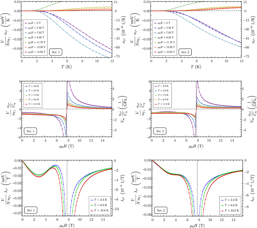
Figure 6: From top to bottom: TE coefficient, Grüneisen ratio and MS plots for the two sets of microscopic parameters given in Table 1. In the plots where the independent variable is the magnetic field, the vertical gridline represents the critical field, $\mu_{\mathrm{0}}H_{\mathrm{c}1}=7.8$ T. In all panels, the left vertical axis gives the theory result normalized to $n_{\Gamma_{1}}$, the right vertical axis shows experimental units using $n_{\Gamma_{1}}=0.9$ GPa^-1 and $V/N\simeq 92.8\,\text{\AA}^{3}$, corresponding to a molar volume $V_{\text{m}}\simeq 55.9\,\text{cm}^{3}/\text{mol}$ Johnson et al. (2015); Park et al. ; Cao et al. (2016). Our semiclassical analysis does not show any of the features interpreted as signatures of an additional regime at intermediate fields above $H_{\mathrm{c}1}$ and thus supports its genuine quantum character.

With that said, we emphasize that neither Set 1 and Set 2, nor any other combination of coefficients we considered in our analysis produces the non-monotonic behavior for $\alpha_{c^{*}}(T)$ at fields in the region between $H_{\mathrm{c}1}$ and $H_{\mathrm{c}2}$, as reported in experiment. Instead, we generally find that $\alpha_{c^{*}}$ increases monotonically at a fixed temperature as $H\rightarrow H_{\mathrm{c}1}^{+}$.

III.3 Grüneisen ratio

Next, we discuss the evolution of the Grüneisen ratio as a function of the magnetic field (see the second row of plots in Fig. 6). Our results show the correct signs above and below $H_{\mathrm{c}1}$, as we have enforced this by a careful analysis of the TE data.

Very close to $H_{\mathrm{c}1}$ magnon excitations proliferate and the non-interacting boson picture underlying LSWT becomes inadequate. Hence, the evolution of $\alpha_{c^{*}}$ and $\alpha_{c^{*}}/C_{\eta}$ through the critical field cannot be reliably computed within our approach. On general grounds Garst and Rosch (2005) we expect that both quantities evolve smoothly at fixed finite $T$ as function of $H$, with the exception of a singularity at $T_{\mathrm{N}}(H)$, crossing zero near $H_{\mathrm{c}1}$.

As noted above, however, we expect our calculations to yield correct results at sufficiently high fields and low temperatures, where the magnon excitation gap is comparable to or larger than $k_{\mathrm{B}}T$. A sample result of the theory for $T=4$ K in comparison with the experimental data, displayed in Fig. 4(b), shows the field dependence of the calculated Grüneisen ratio $\Gamma$ at a fixed low $T$. For a standard direct transition between zigzag and partially polarized phases, the semiclassical result should agree for all fields except very close to the quantum critical point at $H_{\mathrm{c}1}$. The match at low fields is convincing, however, the anomaly of the measured $\Gamma$ in the region above $H_{\mathrm{c}1}$ does not appear compatible with an interpretation in terms of spin-wave theory, suggesting the presence of a genuine quantum regime.

III.4 Magnetostriction

When we move to the results on the MS (bottom row of Fig. 6), we see that both sets of coefficients correctly produce negative values of $\lambda_{c^{*}}$ for the whole range of magnetic fields considered here. However, Set 1 notably leads to large non-monotonic variations around an inflection point in the zigzag phase which are not observed in experiment. The origin of this is in the behavior of the magnon spectrum which evolves in a highly non-trivial fashion with field.

When trying to reduce the intensity of this feature in $\lambda_{c^{*}}$, we verified that it becomes even larger if one, for instance, decreases $n_{K_{1}}$. In fact, without considering variations in $g$, we were unable to find a parameter set capable of smoothing out such a contortion while preserving the main characteristic of the TE coefficient. As far as we could check, this is only accomplished by taking $n_{g}<0$, which motivated us to consider the second set of coefficients.

We recall that LSWT does not produce critical behavior at $T_{\mathrm{N}}$, therefore $\lambda_{c^{*}}(H)$ displays a singularity at $H_{\mathrm{c}1}$ for all temperatures, instead of a singularity at $T_{\mathrm{N}}(H)$.

In regard to the behavior for $H>H_{\mathrm{c}1}$, our results do not bear any resemblance to the kink found in experiment. Together with the absence of a non-monotonic behavior in $\alpha_{c^{*}}$ around $8$ T and the lack of the asymmetric, anomalous Grüneisen ratio above $H_{\mathrm{c}1}$, this suggests that the physics in the regime between $H_{\mathrm{c}1}$ and $H_{\mathrm{c}2}$ cannot be fully accounted for semiclassically, in terms of a continuous field-induced opening of a spin gap alone. This supports the interpretation of our experimental data in terms of an exotic quantum regime in a finite low-temperature region above the quantum critical point at $H_{\mathrm{c}1}$.

IV Discussion

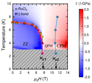
Figure 7: The $T$-$H$ phase diagram of $\alpha$-RuCl₃ as determined in this work for $\vec{H}\parallel$ Ru-Ru bonds ($C_{p}$: yellow squares, TE: red and orange triangles for samples #1 and #2, respectively, MS: pink and blue diamonds). Additionally, the Grüneisen ratio $\Gamma(T,H)$ is shown in color scale (sample 1); these data are the same as in  4 (a). The gray shaded region marks the limits for the color map. In addition to the zigzag (ZZ) ordered state at low fields and the conventional paramagnetic (CPM) state at high fields, our analysis suggests the presence of a third low-temperature regime that is of genuine quantum nature (QPM). The field-driven low-temperature transition at $H_{\mathrm{c}1}$ is continuous, whereas the one at $H_{\mathrm{c}2}$ is either a crossover or a weak first-order transition.

Based on these findings, we construct a temperature-field phase diagram of $\alpha$-RuCl₃ for $\vec{H}\parallel$ Ru-Ru bonds using our experimental thermal expansion, magnetostriction, and specific-heat results. It also includes the Grüneisen ratio $\Gamma(T,H)$ in color scale, interpolated from the experimental data (see Sec. II.3, Fig.  4 (a)). The phase diagram, Fig. 7, shows three distinct low-temperature regimes: (i) the low-field phase with zigzag (ZZ) long-range order terminating at $\mu_{0}H_{\mathrm{c}1}=7.8(2)$ T, (ii) an intermediate quantum paramagnetic (QPM) regime between $\mu_{0}H_{\mathrm{c}1}$ and $\mu_{0}H_{\mathrm{c}2}\approx$ 11 T, and (iii) a conventional paramagnetic (CPM) state with a gapped magnon spectrum and partially polarized spins at high fields above $\mu_{0}H_{\mathrm{c}2}$.

We speculate that the QPM intermediate regime could possibly represent a topological quantum spin liquid as claimed by thermal Hall effect studies Kasahara et al. (2018); Yokoi et al. . Such a phase is not symmetry-distinct from the CPM high-field phase and does not require it to be bounded by a thermal phase transition. Our measurements of the Grüneisen ratio did not show signs of quantum critical scaling near $H_{\mathrm{c}2}$, suggesting the absence of a second-order transition. The transition between the QPM and CPM regimes should therefore be either a crossover or a weak first-order transition. In the latter case, one should expect the transition line at $H_{\mathrm{c}2}$ to terminate at a critical endpoint at finite temperature. We note that the signatures observed around $H_{\mathrm{c}2}$ may in principle also be related to a change in the character of the magnetic excitations as probed by Raman and THz spectroscopy, where indications for magnon bound states have been reported Sahasrabudhe et al. ; Wulferding et al. (2020). Near $H_{\mathrm{c}1}$, on the other hand, the Grüneisen ratio exhibits characteristic quantum critical behavior, confirming the earlier proposal Wolter et al. (2017); dir of a quantum critical point at $\mu_{0}H_{\mathrm{c}1}=7.8(2)$ T and $T=0$.

V Conclusions

Our high-resolution thermal expansion and magnetostriction measurements of $\alpha$-RuCl₃ along the $c^{*}$ axis confirm the field-induced suppression of long-range magnetic order at a critical field of $\mu_{\mathrm{0}}H_{\mathrm{c}1}=7.8(2)$ T, applied parallel to the Ru-Ru bonds, and provide thermodynamic evidence for quantum critical behavior at $H_{\mathrm{c}1}$ from an analysis of the Grüneisen ratio. A clear kink in the measured linear MS coefficient at $\mu_{0}H_{\mathrm{c}2}\approx 11$ T hints at an additional weak first-order phase transition, or a finite-temperature crossover, while an additional second-order phase transition above $H_{\mathrm{c}1}$ can be ruled out. A comparison of our experimental data to calculations using a minimal lattice model, solved in the semiclassical limit via linear spin-wave theory, shows that the behavior at low fields appears well captured by semiclassical theory. In contrast, the regime between $H_{\mathrm{c}1}$ and $H_{\mathrm{c}2}$ is not explained by our minimal spin model. While we cannot draw clear conclusions about the nature of the low-$T$ state at these intermediate fields, we speculate that this could possibly represent the topological quantum spin liquid suggested earlier Kasahara et al. (2018); Yokoi et al. .

Our findings call for a more detailed experimental and theoretical study of the MS (and related quantities) in $\alpha$-RuCl₃ for different in- and out-of-plane field directions. Further theoretical work is needed to investigate possible field-driven transitions in and out of the putative spin liquid in Kitaev-based models Janssen and Vojta (2019) and trying to understand the field dependence of TE and MS in the spin-liquid phase.

Appendix A Sample dependence

The TE was measured on two different samples of $\alpha$-RuCl₃ with similar crystal dimensions ($\sim$ 1 and $\sim$ 0.8 mm in thickness). In this way, sample dependencies due to crystal imperfections were tested. The linear TE coefficient $\alpha_{c^{*}}(T)$ and the corresponding Grüneisen ratio $\Gamma(T)$ on sample #2 are shown in Fig. 8. For comparison, the same observables obtained for sample #1 are shown in Figs. 2 and 4(a) above. The key features are identical, i.e., the sharp peak in $\alpha_{c^{*}}$ at the antiferromagnetic phase transition $T_{\mathrm{N}}=7.2(1)$ K, the sign change of $\alpha_{c^{*}}$ and $\Gamma(T)$ at the critical field $\mu_{0}H_{\mathrm{c}1}=7.8(2)$ T, and the quantum critical signature in $\Gamma(T)$. The shallow maximum in $\alpha_{c^{*}}(T)$ at low temperatures and at $8$ T, however, cannot be observed in sample #2. This is probably related to the reduced thickness of sample #2 leading to even smaller changes in the TE, being at the resolution limit of our experimental setup for these kind of thin 2D van-der-Waals materials. It should be noted, however, that the linear TE coefficient at low temperatures and fields $\mu_{0}H\sim$ 9 T is also slightly increased for sample #2, see inset of Fig. 8(a).

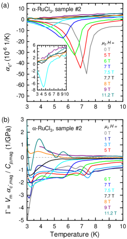
Figure 8: (a) Temperature dependence of the linear TE coefficient perpendicular to the $ab$ plane, $\alpha_{c^{*}}$, for sample #2 of $\alpha$-RuCl₃ for zero and applied magnetic fields $\vec{H}\parallel$ Ru-Ru bonds. The inset shows a zoom of the data for fields close to the critical field $\mu_{0}H_{\mathrm{c}1}=7.8(2)$ T. (b) Grüneisen ratio $\Gamma(T)$ of $\alpha$-RuCl₃ of sample #2 parallel to the Ru-Ru bonds.

Fig. 9 shows the field dependencies of $\alpha_{c^{*},\rm mag}$ and $\Gamma$ for samples #1 and #2, respectively, for different temperatures between $3.5$ K and $10$ K. Note that the measurement accuracy of the two observables is rather different: While the error bar of $\alpha_{c^{*},\rm mag}(H)$ is mainly determined by the reproducibility of our setup and the uncertainty of the subtracted phononic background contribution to $\alpha_{c^{*}}$ (see below), the error of $\Gamma(H)=V_{\rm m}\alpha_{c^{*},\rm mag}/C_{p,\rm mag}$ is influenced by more factors. This can be seen in our data on both samples, where $\Gamma(H)$ displays a large scatter and large errors in the high-field regime above $11.2$ T, where both quantities $\alpha_{c^{*},\rm mag}$ and $C_{p,\rm mag}$ become small due to the spin excitation gap. Still, both data sets (sample #1 and #2) are in good agreement with each other, evidencing the sign change of the linear TE coefficient and of $\Gamma$ at the critical field $\mu_{0}H_{\mathrm{c}1}$. Also the anomalous asymmetric Grüneisen ratio for fields around the critical field and the small absolute values for fields just above $H_{\mathrm{c}1}$ are fully reproduced on both samples. We note that Fig. 4(b) of the main paper displays $\Gamma(H)$ at $4$ K for both samples and at $10$ K for sample #1.

Appendix B Phonon background subtraction

To check the sensitivity of the key features found in the Grüneisen ratio with respect to the choice of the phonon background model for the TE coefficient, we tried two alternative approaches in addition to the scheme discussed in Sec. II.3: (A) We modeled the phononic contribution to the TE using the $14$ T TE data in the gapped high-field state. Although the spin excitation gap is still not large enough to fully gap out magnetic excitations above $\sim 6$ K, the key features of the resulting Grüneisen ratio at low temperatures are robust. (B) Since the phonon contribution to the TE is typically much smaller than that to the specific heat, we neglected this contribution in a first approximation for $T<$ 10 K. A comparison of $\Gamma(H)$ at $4$ K for the different approaches is shown in Fig. 10, emphasizing the robustness of the anomalous behavior of $\Gamma(H)$ for $H>H_{\mathrm{c}1}$ at low $T$.

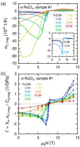
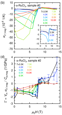
Figure 9: Field dependence of (a,b) the linear TE coefficient $\alpha_{c^{*},\rm mag}$ and (c,d) the Grüneisen ratio $\Gamma$ for (a,c) sample #1 and (b,d) sample #2 in magnetic fields $\vec{H}\parallel$ Ru-Ru bonds for different temperatures between $3.5$ K and $10$ K.

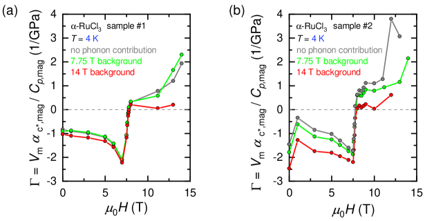
Figure 10: The Grüneisen ratio $\Gamma(H)$ of $\alpha$-RuCl₃ at $T=4$ K as a function of the magnetic field $\vec{H}\parallel$ Ru-Ru bonds using different approximations for the phononic contribution to the TE for (a) sample #1 and (b) sample #2; for details see text.

References

- Nayak et al. (2008) C. Nayak, S. H. Simon, A. Stern, M. Freedman, and S. Das Sarma, Rev. Mod. Phys. 80, 1083 (2008).
- Kitaev (2006) A. Kitaev, Annals of Physics 321, 2 (2006).
- Jackeli and Khaliullin (2009) G. Jackeli and G. Khaliullin, Phys. Rev. Lett. 102, 017205 (2009).
- Chaloupka et al. (2010) J. Chaloupka, G. Jackeli, and G. Khaliullin, Phys. Rev. Lett. 105, 027204 (2010).
- (5) S. Trebst, arXiv:1701.07056 .
- Banerjee et al. (2017) A. Banerjee, J. Yan, J. Knolle, C. A. Bridges, M. B. Stone, M. D. Lumsden, D. G. Mandrus, D. A. Tennant, R. Moessner, and S. E. Nagler, Science 356, 1055 (2017).
- Plumb et al. (2014) K. W. Plumb, J. P. Clancy, L. J. Sandilands, V. V. Shankar, Y. F. Hu, K. S. Burch, H.-Y. Kee, and Y.-J. Kim, Phys. Rev. B 90, 041112(R) (2014).
- Sears et al. (2015) J. A. Sears, M. Songvilay, K. W. Plumb, J. P. Clancy, Y. Qiu, Y. Zhao, D. Parshall, and Y.-J. Kim, Phys. Rev. B 91, 144420 (2015).
- Johnson et al. (2015) R. D. Johnson, S. C. Williams, A. A. Haghighirad, J. Singleton, V. Zapf, P. Manuel, I. I. Mazin, Y. Li, H. O. Jeschke, R. Valentí, and R. Coldea, Phys. Rev. B 92, 235119 (2015).
- Majumder et al. (2015) M. Majumder, M. Schmidt, H. Rosner, A. A. Tsirlin, H. Yasuoka, and M. Baenitz, Phys. Rev. B 91, 180401(R) (2015).
- Kubota et al. (2015) Y. Kubota, H. Tanaka, T. Ono, Y. Narumi, and K. Kindo, Phys. Rev. B 91, 094422 (2015).
- Sinn et al. (2016) S. Sinn, C. H. Kim, B. H. Kim, K. D. Lee, C. J. Won, J. S. Oh, M. Han, Y. J. Chang, N. Hur, H. Sato, B.-G. Park, C. Kim, H.-D. Kim, and T. W. Noh, Sci. Rep. 6, 39544 (2016).
- Ziatdinov et al. (2016) M. Ziatdinov, A. Banerjee, A. Maksov, T. Berlijn, W. Zhou, H. B. Cao, J.-Q. Yan, C. A. Bridges, D. G. Mandrus, S. E. Nagler, A. P. Baddorf, and S. V. Kalinin, Nat. Commun. 7, 13774 (2016).
- Weber et al. (2016) D. Weber, L. M. Schoop, V. Duppel, J. M. Lippmann, J. Nuss, and B. V. Lotsch, Nano Lett. 16, 3578 (2016).
- Yadav et al. (2016) R. Yadav, N. A. Bogdanov, V. M. Katukuri, S. Nishimoto, J. van den Brink, and L. Hozoi, Sci. Rep. 6, 37925 (2016).
- Leahy et al. (2017) I. A. Leahy, C. A. Pocs, P. E. Siegfried, D. Graf, S.-H. Do, K.-Y. Choi, B. Normand, and M. Lee, Phys. Rev. Lett. 118, 187203 (2017).
- Kasahara et al. (2018) Y. Kasahara, T. Ohnishi, Y. Mizukami, O. Tanaka, S. Ma, K. Sugii, N. Kurita, H. Tanaka, J. Nasu, Y. Motome, T. Shibauchi, and Y. Matsuda, Nature (London) 559, 227 (2018).
- Do et al. (2017) S.-H. Do, S.-Y. Park, J. Yoshitake, J. Nasu, Y. Motome, Y. S. Kwon, D. T. Adroja, D. J. Voneshen, K. Kim, T.-H. Jang, J.-H. Park, K.-Y. Choi, and S. Ji, Nat. Phys. 113, 1079 (2017).
- Banerjee et al. (2018) A. Banerjee, P. Lampen-Kelley, J. Knolle, C. Balz, A. A. Aczel, B. Winn, Y. Liu, D. Pajerowski, J. Yan, C. Bridges, A. Savici, B. C. Chakoumakos, M. D. Lumsden, D. A. Tennant, R. Moessner, D. G. Mandrus, and S. E. Nagler, npj Quantum Matter 3, 8 (2018).
- Balz et al. (2019) C. Balz, P. Lampen-Kelley, A. Banerjee, J. Yan, Z. Lu, X. Hu, S. M. Yadav, Y. Takano, Y. Liu, D. A. Tennant, M. D. Lumsden, D. Mandrus, and S. E. Nagler, Phys. Rev. B 100, 060405(R) (2019).
- Sandilands et al. (2015) L. J. Sandilands, Y. Tian, K. W. Plumb, Y.-J. Kim, and K. S. Burch, Phys. Rev. Lett. 114, 147201 (2015).
- Wang et al. (2017) Z. Wang, S. Reschke, D. Hüvonen, S.-H. Do, K.-Y. Choi, M. Gensch, U. Nagel, T. Room, and A. Loidl, Phys. Rev. Lett. 119, 227202 (2017).
- Wellm et al. (2018) C. Wellm, J. Zeisner, A. Alfonsov, A. U. B. Wolter, M. Roslova, A. Isaeva, T. Doert, M. Vojta, B. Büchner, and V. Kataev, Phys. Rev. B 98, 184408 (2018).
- (24) T. Yokoi, S. Ma, Y. Kasahara, S. Kasahara, T. Shibauchi, N. Kurita, H. Tanaka, J. Nasu, Y. Motome, C. Hickey, S. Trebst, and Y. Matsuda, arXiv:2001.01899 .
- Cookmeyer and Moore (2018) J. Cookmeyer and J. E. Moore, Phys. Rev. B 98, 060412(R) (2018).
- Vinkler-Aviv and Rosch (2018) Y. Vinkler-Aviv and A. Rosch, Phys. Rev. X 8, 031032 (2018).
- Jiang et al. (2019) Y.-F. Jiang, T. P. Devereaux, and H.-C. Jiang, Phys. Rev. B 100, 165123 (2019).
- Gordon et al. (2019) J. S. Gordon, A. Catuneanu, E. S. Sørensen, and H.-Y. Kee, Nat. Commun. 10, 2470 (2019).
- Kaib et al. (2019) D. A. S. Kaib, S. M. Winter, and R. Valentí, Phys. Rev. B 100, 144445 (2019).
- Janssen et al. (2017) L. Janssen, E. C. Andrade, and M. Vojta, Phys. Rev. B 96, 064430 (2017).
- Lampen-Kelley et al. (2018) P. Lampen-Kelley, S. Rachel, J. Reuther, J.-Q. Yan, A. Banerjee, C. A. Bridges, H. B. Cao, S. E. Nagler, and D. Mandrus, Phys. Rev. B 98, 100403(R) (2018).
- (32) P. Lampen-Kelley, L. Janssen, E. C. Andrade, S. Rachel, J.-Q. Yan, C. Balz, D. G. Mandrus, S. E. Nagler, and M. Vojta, arXiv:1807.06192 .
- Wolter et al. (2017) A. U. B. Wolter, L. T. Corredor, L. Janssen, K. Nenkov, S. Schönecker, S.-H. Do, K.-Y. Choi, R. Albrecht, J. Hunger, T. Doert, M. Vojta, and B. Büchner, Phys. Rev. B 96, 041405(R) (2017).
- (34) S.-Y. Park, S.-H. Do, K.-Y. Choi, D. Jang, T.-H. Jang, J. Schefer, C.-M. Wu, J. S. Gardner, J. M. S. Park, J.-H. Park, and S. Ji, arXiv:1609.05690 .
- He et al. (2018) M. He, X. Wang, L. Wang, F. Hardy, T. Wolf, P. Adelmann, T. Bräckel, Y. Su, and C. Meingast, J. Phys.: Condens. Matter 30, 385702 (2018).
- Baek et al. (2017) S.-H. Baek, S.-H. Do, K.-Y. Choi, Y. S. Kwon, A. U. B. Wolter, S. Nishimoto, J. van den Brink, and B. Büchner, Phys. Rev. Lett. 119, 037201 (2017).
- Hentrich et al. (2018) R. Hentrich, A. U. B. Wolter, X. Zotos, W. Brenig, D. Nowak, A. Isaeva, T. Doert, A. Banerjee, P. Lampen-Kelley, D. G. Mandrus, S. E. Nagler, J. Sears, Y.-J. Kim, B. Büchner, and C. Hess, Phys. Rev. Lett. 120, 117204 (2018).
- Zhu et al. (2003) L. Zhu, M. Garst, A. Rosch, and Q. Si, Phys. Rev. Lett. 91, 066404 (2003).
- Garst and Rosch (2005) M. Garst and A. Rosch, Phys. Rev. B 72, 205129 (2005).
- Cao et al. (2016) H. B. Cao, A. Banerjee, J.-Q. Yan, C. A. Bridges, M. D. Lumsden, D. G. Mandrus, D. A. Tennant, B. C. Chakoumakos, and S. E. Nagler, Phys. Rev. B 93, 134423 (2016).
- Widmann et al. (2019) S. Widmann, V. Tsurkan, D. A. Prishchenko, V. G. Mazurenko, A. A. Tsirlin, and A. Loidl, Phys. Rev. B 99, 094415 (2019).
- Lindemann (1910) F. A. Lindemann, Phys. Z. 11, 609 (1910).
- Jansa et al. (2018) N. Jansa, A. Zorko, M. Gomilsek, M. Pregelj, K. W. Krämer, D. Biner, A. Biffin, C. Rüegg, and M. Klanjsek, Nat. Phys. 14, 786 (2018).
- Winter et al. (2016) S. M. Winter, Y. Li, H. O. Jeschke, and R. Valentí, Phys. Rev. B 93, 214431 (2016).
- Landau and Lifshitz (1959) L. D. Landau and E. M. Lifshitz, Course of Theoretical Physics Vol 7: Theory and Elasticity (Pergamon Press, Oxford, UK, 1959).
- Chaikin and Lubensky (2000) P. Chaikin and T. C. Lubensky, Principles of Condensed Matter Physics (Cambridge University Press, Cambridge, UK, 2000).
- Barrera et al. (2005) G. D. Barrera, J. A. O. Bruno, T. H. K. Barron, and N. L. Allan, J. Phys.: Condens. Matter 17, R217 (2005).
- (48) We note that, according to standard sign conventions Chaikin and Lubensky (2000), positive stress leads to an elongation (i.e. to positive strain) along a given axis. Thus, stress and uniaxial pressure have opposite signs.
- Yadav et al. (2018) R. Yadav, S. Rachel, L. Hozoi, J. van den Brink, and G. Jackeli, Phys. Rev. B 98, 121107 (2018).
- Holstein and Primakoff (1940) T. Holstein and H. Primakoff, Phys. Rev. 58, 1098 (1940).
- Blaizot and Ripka (1986) J. P. Blaizot and G. Ripka, Quantum Theory of Finite Systems (MIT Press, Cambridge, MA, USA, 1986).
- Rau et al. (2018) J. Rau, P. A. McClarty, and R. Moessner, Phys. Rev. Lett. 121, 237201 (2018).
- Janssen and Vojta (2019) L. Janssen and M. Vojta, J. Phys.: Condens. Matter 31, 423002 (2019).
- Winter et al. (2017) S. M. Winter, K. Riedl, P. A. Maksimov, A. L. Chernyshev, A. Honecker, and R. Valentí, Nat. Commun. 8, 1152 (2017).
- Winter et al. (2018) S. M. Winter, K. Riedl, D. Kaib, R. Coldea, and R. Valentí, Phys. Rev. Lett. 120, 077203 (2018).
- Winter et al. (2017) S. M. Winter, A. A. Tsirlin, M. Daghofer, J. van den Brink, Y. Singh, P. Gegenwart, and R. Valentí, Journal of Physics Condensed Matter 29, 493002 (2017).
- (57) L. Janssen, S. Koch, and M. Vojta, arXiv:2002.11727 .
- (58) A. Sahasrabudhe, D. A. S. Kaib, S. Reschke, R. German, T. C. Koethe, J. Buhot, D. Kamenskyi, C. Hickey, P. Becker, V. Tsurkan, A. Loidl, S.-H. Do, K. Y. Choi, M. Grüninger, S. M. Winter, Z. Wang, R. Valentí, and P. H. M. van Loosdrecht, arXiv:1908.11617 .
- Wulferding et al. (2020) D. Wulferding, Y. Choi, S.-H. Do, C. H. Lee, P. Lemmens, C. Faugeras, Y. Gallais, and K.-Y. Choi, Nat. Comun. 11, 1603 (2020).
- (60) Note that the measurements of Ref. Wolter et al. (2017) were done for an arbitrary in-plane direction, while in the current work, we have aligned the magnetic field along the Ru-Ru bonds. In this setup, the in-plane critical field is largest, see Ref. Janssen et al. (2017).